

Introduction
There is growing interest in the Nordic countries to improve grassland yields and quality by means of increased precision in forage production. Updated information on the prevailing field situation is necessary, in particular robust estimates on yields, in order to support the farmers in their management decisions. Recently emerged UAVs and hyperspectral imaging systems may play a major role in rapid and non-destructive sampling of such information (Schut et al., Reference Schut, van der Heijden, Hoving, Stienezen, van Evert and Meuleman2006). We have already shown the potential of hyperspectral aerial imaging and multivariate regression techniques for the determination of spring wheat grain yield (Øvergaard et al., Reference Øvergaard, Isaksson, Kvaal and Korsæth2010; Kusnierek and Korsaeth, Reference Kusnierek and Korsaeth2015). In this article, we present our first results for the estimation of grassland yields.
Materials and methods
Field trials
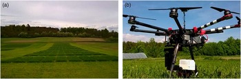
In this study, we utilized an ongoing variety field trial in order to assess the spectral signature of five different grassland species, cultivated as monocrops (Phleum pratense L., Lolium perenne L., Festuca pratensis, Trifolium pratense L., Trifolium repens L.). The trial was arranged as a complete randomized block design with three replicates. In addition, we established a field trial in 2015 with a typical mixed sward (seed mix: 77% Phleum pratense L., 20% Festuca pratensis, 3% Trifolium pratense L.) as a split-plot design with five replicates (Fig. 1a). To ensure variation in grass yields, we used fertilizer rate as a factor on the major plots (either 130, 200, 270 kg N ha−1), and time of harvest on the sub-plots. For the first cut, an early (E) harvest was performed a week earlier than the normal (N) harvest, which corresponded to approximately 90 growing degree days (GDD, base temperature 0°C). We managed the field trials as a typical Norwegian 3-cut regime, with the first cut at the early heading of Phleum pratense L., the second cut about 600 GDD later, and the third cut in the middle of September, depending on the weather conditions. We focused on the first cut of the monocrop trial and the two first cuts of the mixed sward trial, only. All measurements were performed in the 2016 season in the first ley year.
A mixed sward field trial with 120 plots (a). The modified DJI S1000+ with an attached 3-axes stabilized gimbal and the Rikola hyperspectral imager (b).

Sensor and sensor platform
We utilized the Rikola hyperspectral camera to measure the grass canopy reflection at a nadir view. The Rikola imager is a small and robust snapshot camera with a resolution of 1 megapixel and a weight of 720 g (Rikola, Reference Rikola2017). We configured it to register 29 wavebands in the range from 455 to 780 nm with full width half maxima (FWHM) of 10 to 20 nm. As we expected higher correlations of the near-infrared reflection with the grass yield, we chose spectral resolutions from 5 nm for this part of the electromagnetic spectrum to around 20 nm for the visible part. As sensor platform, we used a DJI S1000+ multi-rotor UAV. We modified it to carry a high-precision 3-axes stabilized gimbal, on which we mounted the Rikola camera. With this setup, the UAV had a take-off weight of around 10 kg, which allowed for a flight time of 12 min (Fig. 1b).
Measurements
In the beginning of the vegetation period, we conducted a topographic survey, using a Trimble Geo7X real-time kinematic global navigation satellite system (RTK-GNSS) receiver and a dense measurement raster, to generate a digital terrain model (DTM) of the trials’ locations. Moreover, we staked out ground control points (GCP) and marked their positions with iron tubes, which we used as mounts for black and white reference targets. Prior to each harvest, we measured the field with the Rikola camera hyperspectrally at a scheduled flight altitude of 50 m. This was always performed during clear skies with stable weather conditions. Before take-off, we captured a dark current image by closing the camera’s optics, and a grey reference image by pointing the camera towards a defined spectral reference panel (Sphere Optics, Reflectivity 50%). For the grass harvest, we used an experimental plot harvester to weigh the fresh matter (FM) of the plots. In addition, we took samples of each plot and determined their FM weight. Subsequently, we dried the samples for 48 hours at 60 °C for dry matter (DM) and weighed them again to infer on each plots’ DM content.
Data pre-processing
We performed data pre-processing for each flight mission individually in an 11-step procedure. In the first step, we corrected the Rikola imagery for the sensor’s dark current and removed the lens’ vignetting effect. In the second step, we divided each image by its corresponding grey reference image to remove any radiometric inequalities of the sensors’ pixels and to obtain a reflectance image, carrying the canopy’s relative reflection values. In the third step, we used the 3D reconstruction software Agisoft Photoscan Professional to process a crop surface model (CSM) and accurate hyperspectral orthoimages. This was obtained by removing the lens’ geometric distortion effects for each image and waveband. After that, we processed an orthoimage for each waveband individually using the GCP coordinates for the determination of the exterior orientation. Then, we generated the CSM by selecting the 530 nm waveband as it showed a high level of contrast. For further processing, we used the statistical computation software R. In the fourth step, we performed an additional grey reference correction on the orthoimages in case the resulting wavebands showed inaccuracies in the desired 50% reflectance at the location of the grey reference target. In the fifth step, we co-registered the resulting orthoimages to a hyperspectral orthoimage cube by using their spatial reference. In the sixth step, the RTK-GNSS measurements of our topographic survey were utilized to create a DTM, applying the inverse distance weighted interpolation algorithm. In the seventh step, we subtracted the DTM from the CSM to produce an elevation model with plant height information. We then overlaid the resulting elevation model with a geographical vector data set, containing the field trials’ plot locations, and extracted the average plant height for each plot in the eighth step. In the ninth step, we extracted the radiometric information from each pixel of the hyperspectral orthoimage cube and calculated an average spectrum for each plot. In the tenth step, we normalized these spectra individually to a mean reflectance value of 1 to account for possible illumination changes during image acquisition. Finally, in the eleventh step, we centered the spectra for further analysis.
Modeling
All spectra of the monocrop field trial were first pooled to perform a combined analysis of all species and varieties. We utilized a principal component analysis (PCA) to search for dissimilarities between the species in terms of spectral signature. Then, we analyzed the spectra of the mixed sward field trial for their potential use to estimate grass yields (DM) overall and for each harvest date individually. To do so, we fitted several powered partial least squares (PPLS) regression models to the spectra while controlling the range for the power optimization parameter γ from a lower limit of 0.5 to an upper limit of 0.99 (Indahl, Reference Indahl2005). We selected the number of PPLS factors by using the factor with a local minimum of the root-mean-square error (RMSE) as criterion to avoid overfitting. From the resulting PPLS models, we selected the dominant wavebands for testing with multiple linear regression (MLR) models. We corrected the MLR models by removing the insignificant wavebands from the independent variable matrix. Consequently, we reduced all MLR to simple linear regression (SLR) models, except for the pooled dataset. In addition to that, we fitted some SLR models, based on the popular normalized difference vegetation index (NDVI), the red-edge inflection point (REIP), the plant height (PH), and the grassland index (GrassI). We calculated these values as shown in Table 1.
Calculation formula for the independent variables of the SLR models

We corrected all regression models for outliers, which we defined as samples with absolute residual errors of more than three standard deviations. All models were evaluated by 10-fold randomized cross-validation, which we repeated 1001 times. We then selected the model with the median RMSE of cross-validation.
Results
Data pre-processing
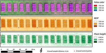
The processed orthoimages and the CSM showed a resulting ground sample distance (GSD) of 4 cm per pixel. The overall 3D residual errors of the GCP locations were around 5 cm (RMSE). Figure 2 illustrates selected results for the second cut of the mixed sward field trial.
False color orthoimage, REIP orthoimage, and PH orthoimage of the second cut of the mixed sward field trial.

Modeling
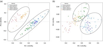
Figure 3 shows the score plots for the first three principal components (PC) of the PCA. PC 1 and 2, which together explained 99.1% of the dataset’s variance, revealed distinct reflectance differences between the grass species on the one and the clover species on the other hand (Fig. 3a). The clusters were highly influenced by the red-edge wavebands from 725 to 745 nm.
Score plots for the PCA’s first three PCs. PC 1 and 2 show two predominant clusters of the three grass and the two clover species (a). PC 1 and 3 show two clusters to distinguish Phleum pratense L. from Festuca pratensis and Lolium perenne L. (b).

PC 3 explained only 0.5% of the variance but carried additional information to distinguish Phleum pratense L. from Festuca pratensis and Lolium perenne L. (Fig. 3b). In the corresponding loadings, we identified reflectance information in the green wavebands from 530 to 575 nm as the main contributor. The PCA did not reveal pronounced variety differences.
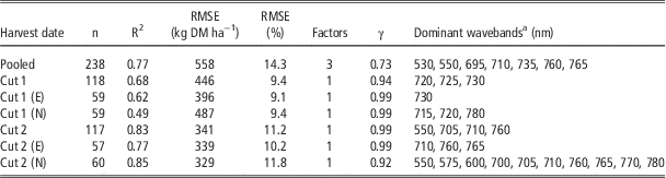
In Table 2, we present the cross-validated PPLS models, which obtained the lowest RMSE values for each harvest date and for the pooled data. The relative RMSEs of prediction ranged from 9.1 to 11.8% (329 to 487 kg DM ha−1) for the individual harvest dates and 14.3% (558 kg DM ha−1) for a generalized model, when pooling the data from all harvest dates. Except for the pooled dataset, the PPLS models contained only one factor, and the γ value was in the upper range. More factors in the PPLS models did not improve the model performance significantly.
Cross-validated PPLS model results at different harvest dates

a Dominant in terms of high absolute regression coefficients
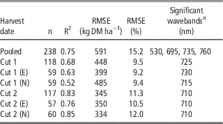
Table 3 shows the results of the linear regression models, using the dominant wavebands from the PPLS regressions as predictors. Only wavebands (predictors), which contributed significantly to the MLR models, were included in the final models. The relative RMSEs of prediction ranged from 9.2 to 12.0% (334 to 485 kgDMha−1) for the individual harvest dates and 15.2% (591 kgDMha−1) for the generalized model. The regression models performed almost equally well as the PPLS models and even slightly better for Cut 1 (N). All the models, predicting yields for each harvest date individually, contained only one significant waveband as a predictor. The wavebands, which were used as a predictor, shifted from longer wavelengths (715–730 nm) for the first cut models to a shorter wavelength (710 nm) for the second cut models (Table 3).
Cross-validated SLR/MLR model results at different harvest dates, using PPLS regressions for the selection of potential predictors

a Significant wavebands (p≤0.05), selected from dominant PPLS wavebands
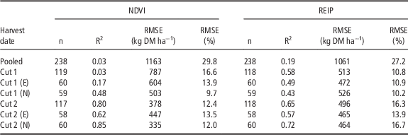
The SLR models, based on the vegetation indices NDVI and REIP (Table 4), performed poorly on the pooled dataset (RMSEs of 29.8 and 27.2%, 1163 and 1061 kg DM ha−1). The predictive ability of the NDVI was also low for the early first cut (E) and for the pooled data (Cut 1), with relative RMSEs of 13.9 and 16.6% (604 and 787 kg DM ha−1), respectively. The predictive accuracy increased for the other harvest dates (RMSEs from 9.7 to 13.5%, 335 to 503 kg DM ha−1). The REIP achieved higher accuracies for the first cut (RMSEs from 10.2 to 10.8%, 472 to 526 kg DM ha−1), but lower ones for the second cut (RMSEs from 13.9 to 16.7%, 464 to 496 kg DM ha−1). The approach using either PPLS regression directly or a SLR/MLR, following a PPLS-based selection of predictors, was superior to the SLR with either of these two vegetation indices.
Cross-validated SLR model results at different harvest dates with NDVI and REIP as predictors

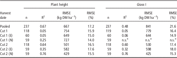
Using the plant height as a predictor (Table 5), the SLR models obtained an overall relative RMSE of 17.2% (667 kg DM ha−1) but performed poorly on the first cut (RMSEs from 14.0 to 15.9%, 649 to 754 kg DM ha−1). The predictive ability of the plant height increased for the second cut (RMSEs from 15.5 to 17.6%, 429 to 582 kg DM ha−1), but did not outperform the other regression models. For the first and second cut, the SLR models, using the GrassI as a predictor, performed similar to the models, using plant height (Table 5). For the pooled dataset, the SLR model, using the GrassI, performed much worse (RMSE of 21.6%, 841 kg DM ha−1).
Cross-validated SLR model results at different harvest dates with plant height and Grass I as predictors

a Not significant (p>0.05)
Discussion
The PCA, which was based on the reflectance signature of the species in monoculture, showed a clean clustering of two groups, with the erectophil grasses in one group and the planophil clover leaves in the other. The most contributing wavelengths to this separation were located in the red-edge region of the electromagnetic spectrum, which is known to be chlorophyll and nitrogen sensitive. However, in this case, we expect that the leaf shape and the canopy structure were predominant factors for governing the observed reflectance pattern. Since there were distinct reflectance differences between the grass and the clover species, we assume that, in terms of modeling, it may be beneficial to aim at a stable clover level inside a sward, as different clover proportions may require different modeling strategies.
The PPLS approach achieved the highest predictive ability in terms of DM yields, and performed slightly better than that reported by Schut et al. (Reference Schut, van der Heijden, Hoving, Stienezen, van Evert and Meuleman2006) in a comparable study. We followed a relatively conservative approach for factor selection and identified the potential for using an overall model for all harvest dates. Individual models for the different harvest strategies resulted, however, in higher accuracies and they predominantly relied on the reflectance in the red and red-edge wavebands.
Interestingly, we obtained almost identical model performance by using only a few bands when utilizing PPLS for variable (predictor) selection, followed by SLR/MLR. These wavebands may thus have the potential to carry sufficient information to serve as a basis for a new vegetation index for DM yield estimation. Such a development requires, however, more data for a robust model calibration.
The results of the popular vegetation indices NDVI and REIP did not outperform those of the preceding modeling strategies. The NDVI appeared to be saturated at the first harvest dates and did not achieve an acceptable prediction level. The REIP had an intermediate performance at all harvest dates compared to the other strategies.
Plant height could be used to model DM for the pooled dataset and the second cut with a reasonable performance, but had almost no predictive ability for the first harvest dates. The GrassI, containing information on both plant height and RGB-reflectance, did not improve the prediction accuracy.
Conclusions
Airborne imaging spectroscopy is an appropriate method for in-season grassland yield estimation. We found distinct reflectance differences, especially between the erectophil grass and the planophil clover leaves, which show that the proportion of clover in a grass sward may affect the model accuracy significantly. The PPLS achieved the highest predictive ability in terms of DM yield modeling, but MLR models, containing only a few wavebands as predictors, performed almost equally well. We believe that a reflectance-independent estimator for biomass and/or canopy density may improve the grass yield prediction, but plant height appears not to be the solution.
Acknowledgements
This work is part of the project “Use of remote sensing for increased precision in forage production”, which is funded by the Fondet for jordbruk og matindustri. We profoundly thank Jan Thomsen for the technical assistance in the field and Wendy Waalen for the linguistic corrections.