1. Introduction
With advancements in control science, aeronautical engineering, and other disciplines, unmanned aerial vehicles (UAVs) have rapidly developed and are widely used across various fields, including film and television aerial photography, agricultural and forestry applications, geological exploration, and logistics and transportation. In recent years, the operation of UAVs in complex low-altitude environments, such as urban areas and mountainous regions, has garnered significant attention [Reference Zhang, Xu and Shan1, Reference Garibeh, Alshorman, Jaradat, Younes and Khaleel2]. These environments pose unique challenges due to the low flight altitudes, which limit the ability to obtain clear mapping information from satellite remote sensing. Additionally, the irregular distribution of obstacles, the varying heights of these obstacles, and the fluctuating widths of flight corridor pose significant challenges for UAV safety.
Agile fixed-wing UAVs are a type of UAV with aerobatic capabilities, characterized by a high thrust-to-weight ratio, strong rudder effect, and low aspect ratio [Reference Khan and Nahon3]. Compared to rotary-wing UAVs, agile fixed-wing UAVs offer faster flight speeds and superior endurance. In contrast to traditional fixed-wing UAVs, agile fixed-wing UAVs have enhanced maneuvering capabilities, including large-angle hovering, very low-speed flight, and significant lateral maneuvers [Reference Cheng and Pei4–Reference Kumar, Arya and Joshi6]. Hence, it is feasible to consider leveraging the superior lateral flight capabilities of agile fixed-wing UAVs to enhance the safety of UAV missions performed in complex low-altitude environments.
Motion planning is a key technology for enabling autonomous flight in UAVs. It involves determining an optimal or near-optimal path or trajectory that considers the constraints of the UAV, the mission, and the environment to achieve a specific objective [Reference Wu7]. Depending on the planning space, motion planning can be classified into path planning, which operates in discrete state space; trajectory planning, which operates in continuous curve parameter space; and hybrid planning, which involves planning in the space of trajectories or action primitives [Reference Dong, He, Song and Sun8–Reference Israr, Ali, Alkhammash and Jussila10].
Path planning refers to the process of planning a path in a space that contains only spatial information [Reference Jones, Djahel and Welsh11]. Algorithms of path planning include search-based, sampling-based, artificial potential field-based, intelligent optimization-based, and reinforcement learning-based algorithms. Search-based algorithms can guarantee the optimality and completeness of the solution but may encounter the curse of dimensionality. Artificial potential field-based algorithms are prone to getting trapped in local optima, while intelligent optimization-based algorithms often exhibit slow convergence rates. Most reinforcement learning-based algorithms are still in the simulation phase. Sampling-based path planning algorithms perform path searches by randomly selecting sample points in the state space and connecting these points according to specific rules to form a graph or tree structure. One of the most representative algorithms is the Rapidly exploring Random Tree (RRT), which is probabilistically complete but not necessarily optimal [Reference Zammit and v. Kampen12]. Many algorithms have been developed based on RRT. RRT* incorporates the process of re-selecting parent nodes and rewiring the tree, making it asymptotically optimal [Reference Karaman and Frazzoli13, Reference Gao, Li, Liu, Ge and Song14]. The Informed RRT* restricts the sampling points to an ellipse centered around the start and end points, thereby enhancing sampling efficiency [Reference Gammell, Srinivasa and Srinivasa15]. The Batch Informed Trees (BIT*) combines the advantages of the sampling strategies from the Fast Marching Trees and the Informed RRT* by batching points within the ellipse and introduces heuristic approaches to evaluate path costs, significantly improving efficiency [Reference Gammell, Barfoot and Srinivasa16].
Trajectory planning encompasses not only time information but also takes into account the kinematic and dynamic constraints of the UAV [Reference Guo, Guo, Wang, Yao, Li and L.17, Reference Zhu, He and Sun18]. It typically utilizes initial points provided by path planning to enhance the success rate and speed of solutions. Trajectory representations include segmented polynomial, Dubins, B-spline, and Minimum Control Effort (MINCO) [Reference Mellinger and Kumar19–Reference Wang, Zhou, Xu and Gao22]. Obstacles are usually modeled as inequality constraints (hard constraints) or cost functions (soft constraints) in trajectory planning. Hard constraint methods can ensure safety but are often difficult and slow to solve, whereas soft constraint methods are typically numerically stable and easier to resolve [Reference Bry, Richter, Bachrach and Roy23]. Tal derived the global differential flatness properties of a VTOL fixed-wing UAV, generating polynomial trajectories in flat space to achieve agile maneuvering flights, including lateral uncoordinated flight and inverted flight [Reference Tal, Ryou and Karaman24]. Bry proposed a Dubins-Polynomial trajectory based on differential flatness properties to enable high-speed flight of fixed-wing UAVs in underground garages [Reference Bry, Richter, Bachrach and Roy23]. Based on B-spline, Gao proposed an EGO planner for real-time planning of autonomous flights in environments with unknown obstacles [Reference Zhou, Wang, Ye, Xu and Gao25]. Wang proposed the minimum control effort trajectory that can simultaneously optimize time and space, achieving swarm flights of rotary-wing UAVs in dense bamboo forest environments [Reference Wang, Zhou, Xu and Gao22, Reference Zhou, Wen, Wang and Gao26].
The core concept of hybrid planning is to combine trajectories or motion segments that satisfy dynamic characteristics to form a longer continuous trajectory or motion sequence [Reference Zhang27]. For autonomous flight missions in complex low-altitude environments, there are numerous constraints involved, and the aircraft may need to perform maneuvering flight actions. The solutions for trajectory libraries or motion primitives of agile fixed-wing UAVs differ significantly from those of conventional fixed-wing UAVs. Moreover, hybrid planning need to solve additional optimization problems, which often results in poor real-time performance. Thus, the hybrid planning may not fulfill our requirements.
In practice, the motion planning framework that combines front-end path planning and back-end trajectory planning has been widely applied. The challenge in front-end path planning is to quickly obtain high-quality solutions. Despite the advanced sampling-based path planning algorithm BIT* demonstrating good performance, issues such as its slow initial solution computation speed still limit its application in complex low-altitude environments. The challenge in back-end trajectory planning is to derive a flyable trajectory for the UAV in real time, considering mission time, UAV dynamic performance, and flight safety. Currently, most fixed-wing UAV trajectory planning validated through actual flight experiments primarily focuses on the UAV’s position without considering its attitude, which limits the adaptability of the UAV in narrow corridors within complex low-altitude environments. Additionally, some trajectory planning methods are based on a coordinated turning model of fixed-wing UAVs to derive differential flatness [Reference Liu, Li and Zou28]. In summary, motion planning for fixed-wing UAVs in complex low-altitude environments remains challenging.
This paper proposes a motion planning method for small agile fixed-wing UAVs operating in complex low-altitude environments. At the path planning layer, to address the issues of slow solution speed and low solution quality of the BIT algorithm that fail to meet environmental requirements, we introduce an Improved Batch Informed Trees (IBIT*) algorithm, which enhances computational speed while improving the quality of the planned paths. In the trajectory planning layer, we first decouple the roll angle of the UAV from its 3-D position based on the lateral maneuverability of agile fixed-wing UAVs, thereby enhancing the UAV’s ability to navigate through narrow corridors. Subsequently, we utilize the MINCO approach to represent the trajectory and design a differentiable penalty function to account for the constraints imposed by the UAV’s dynamic performance. Experimental results demonstrate that the proposed motion planning method can rapidly generate reasonable flight trajectories with roll angles.
The remainder of this paper is organized as follows. Section 2 introduces the designed motion planning framework. Section 3 presents the IBIT* algorithm. Section 4 discusses the trajectory planning problem for agile fixed-wing UAVs. Section 5 describes the flight experiment. Finally, Section 6 provides a summary of the entire paper.
2. Agile fixed-wing UAV motion planning framework
The complex low-altitude environment is subject to numerous constraints, including time, safety, smoothness, and the dynamic performance of the UAV. Among these, safety constraints differ significantly from those in ordinary environments. In certain areas of the complex low-altitude environment, UAVs may need to fly laterally at a specific roll angle to pass through safely. Given the robust lateral flight capability of agile fixed-wing UAVs, we can treat the roll angle as a degree of freedom specifically dedicated to obstacle avoidance. This implies that the outcome of the motion planning process will be a trajectory with an associated roll angle [Reference Ramírez and Nahon29].
Motion planning framework.

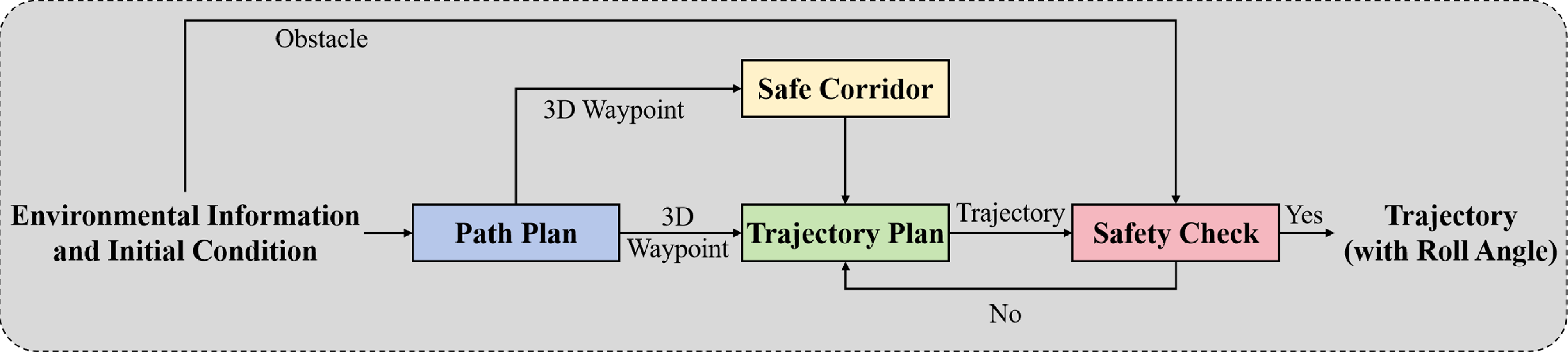
The agile fixed-wing UAV motion planning framework designed for complex low-altitude environments is illustrated in Figure 1. This framework comprises four steps: path planning, Safety Flight Corridor (SFC) generation, trajectory planning, and safety detection, with a primary focus on path planning and trajectory planning in this paper. The SFC is generated based on the method proposed in [Reference Ma, Wang, Ma, Liu and Niu35]. The motion planning framework first conducts path planning to compute a set of discrete 3-D waypoints; then, to enhance the real-time performance of trajectory planning, the SFC is constructed based on the results of path planning to narrow down the planning space. Subsequently, in trajectory planning, constraints such as safety, smoothness, and dynamic performance are considered to generate a trajectory online that meets these constraints. Finally, a safety loop closure check is conducted on the trajectory to further ensure its safety.
3. Improved Batch Informed Trees based path planning
3.1. The drawbacks of the BIT* in complex low-altitude environments
In complex low-altitude environments, autonomous UAVs require real-time path planning based on local environmental data, demanding planners to quickly generate high-quality paths. Optimal solutions aren’t essential for two reasons: (1) Local planning inherently lacks global environmental awareness, making true optimization unattainable and (2) sampling-based planning methods typically converge to near-optimal solutions within reasonable iterations, rendering excessive time spent on perfect paths unjustified.
BIT* algorithm integrates FMT* and Informed RRT* strengths with heuristics for efficiency, yet faces three key limitations in complex low-altitude environments:
-
1) Inefficient uniform sampling: BIT* relies on uniform sampling before and after finding initial solutions (state-space-wide then ellipsoid-restricted). This approach generates redundant clustered points that increase computation without improving solutions.
-
2) Slow initial solution discovery: By retaining only quality-enhancing samples, BIT* experiences delayed initial path finding. This prolongs uniform sampling cycles, severely degrading performance.
-
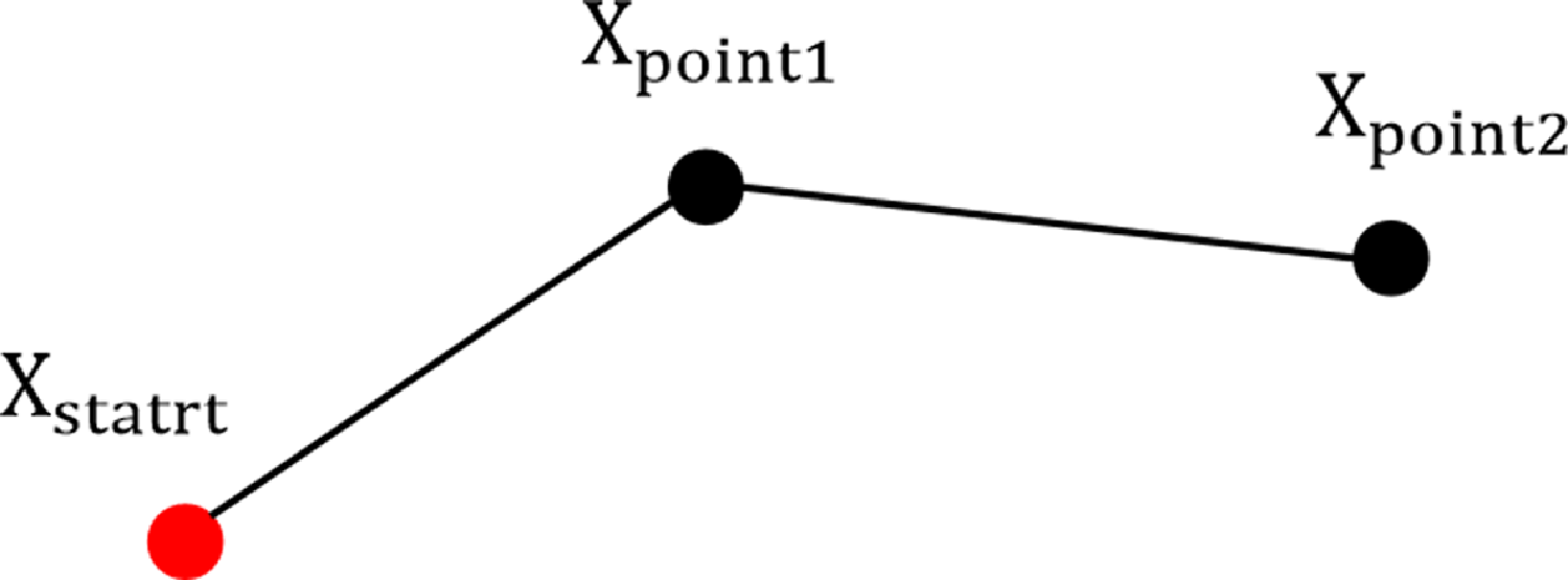
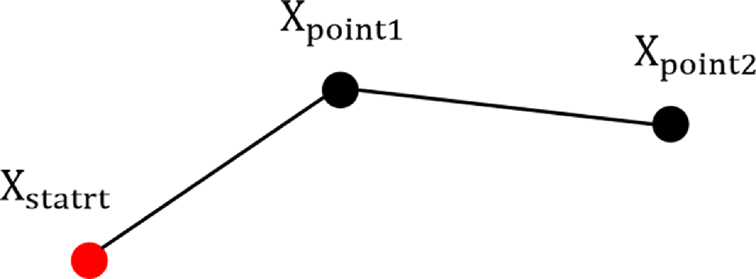
3) Suboptimal pruning mechanism: While pruning non-contributing vertices improves solution quality, BIT* delays pruning until both vertex/edge queues empty. The absence of parent node reselection creates suboptimal “Polyline Segments” (Figure 2), further compromising solution quality.
Polyline segment.
3.2. Improved Batch Informed Trees
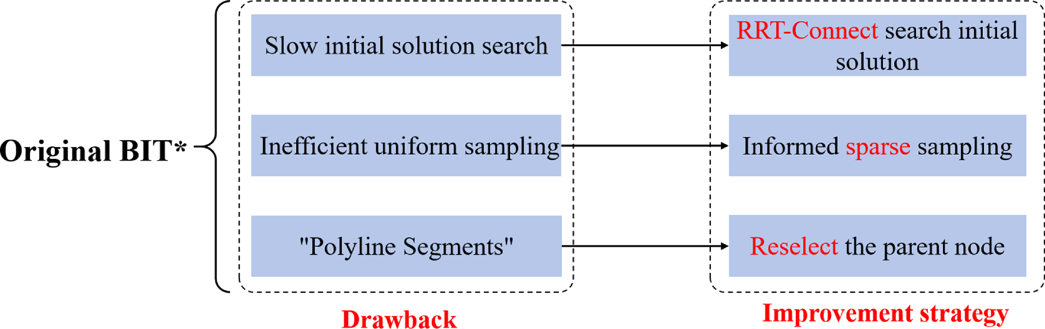
To address the three issues present in BIT*, the Improved Batch Informed Trees (IBIT*) is proposed, with its improvement strategies illustrated in Figure 3.
Three improvement strategies for the BIT*.

To resolve slow initial solution searches, we use RRT-Connect for rapid solution discovery [Reference Chang, Dong and Li30]. This single-query algorithm builds two trees from the start and goal, alternately extending toward each other to achieve accelerated exploration. While RRT-Connect does not ensure optimality, we leverage its speed advantage exclusively. Being a classic algorithm, its implementation details are omitted here.
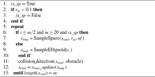
To improve uniform sampling inefficiency, we implement an informed sparse sampling strategy (detailed in Algorithm 1). Its core step (
 $\text{SampleSpare}({{x}_{rand}},{{r}_{sp}},nf)$
) inputs sparse radius
 ${r}_{sp}$
, current points
 ${x}_{rand}$
, and allowable failures
 $nf$
, outputting a new point.
 $\text{SampleSpare}({{x}_{rand}},{{r}_{sp}},nf)$
first samples within the informed ellipsoid, then checks distances to
 ${x}_{rand}$
. If all exceed
 ${r}_{sp}$
, it outputs the point; otherwise, it resamples. After
 $nf$
consecutive failures, it returns the last valid sample. Parameter
 $nf$
prevents excessive iterations to save resources. Note: Line 9 in Algorithm 1 handles uniform sampling, while line 11 performs collision detection.
imSample (m,x start,X goal,c i) Informed sparse sampling

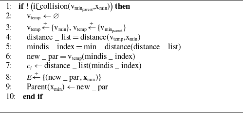
To tackle inadequate pruning, we propose a parent node reselection method, detailed in Algorithm 2. This process is triggered whenever a new node and edge are added to the search tree. The decision to reassign the parent of node
 ${{\mathbf v}}_{\min }$
as the parent of node
 ${{\mathbf x}}_{\min }$
hinges on safety (evaluating obstacles between
 ${{\mathbf v}}_{\min }$
and
 ${{\mathbf x}}_{\min }$
) and the potential to reduce cost from
 ${{\mathbf x}}_{\min }$
back to the origin.
rc_parent(vmin,xmin) Reselect the parent node

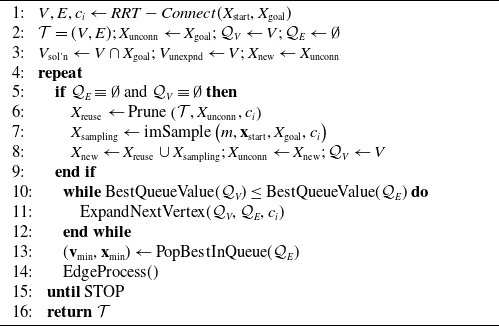
The pseudocode for IBIT* is shown in Algorithm 3. The vertex expansion step
 ${\text{Expand}}\text{NextVertex } ({\mathcal{Q}}_{V},{\mathcal{Q}}_{E},c_i)$
and graph pruning step
 $\text{Prune }({\mathcal{T}},X_{\text{unconn}},c_i)$
are the same as in BIT*, so they won’t be discussed here. The core steps of IBIT* include:
1) Initialization: Initialize start state
 ${x}_{start}$
, goal state
 ${x}_{goal}$
, tree
 $T\,:\!=\, (V,E)$
, disconnected state set
 ${X}_{unconn}$
, vertex expansion queue
 ${Q}_{V}$
, and edge evaluation queue
 ${Q}_{E}$
. Also define goal region vertices
 ${V}_{sol'n}$
and unexpanded vertex variables
 ${V}_{unexpnd}$
.
2) Batch Sampling: During new batch initialization, the queue resets. Samples and trees are pruned to remove states incapable of enhancing solutions. New samples are then collected from subproblems with superior solutions (
 $\text{Sample }(m,{\mathbf x}_{\text{start}},X_{\text{goal}},c_i)$
).
3) Edge Selection: The tree grows (
 $\text{Expand}\text{NextVertex }({\mathcal {Q}}_V,{\mathcal {Q}}_E,c_i)$
) by processing edges sorted by ascending estimated costs. When multiple edges share identical estimates, priority is given to those with minimal current cost to the source vertex (
 $\text{PopBest InQueue }({\mathcal {Q}}_E)$
).
4) Edge Processing: Heuristics accelerate edge processing and delay actual cost computations. Functions
 $\widehat {g}(x)$
and
 $\widehat {h}(x)$
estimate forward costs (start to
 $x\in X$
) and backward costs (to goal), respectively. Parent node
 $\text{rc }\!\!\_\!\!\text{ parent(}{{\text{v}}_{\text{min}}}\text{,}{{\text{x}}_{\text{min}}}\text{)}$
reselection is embedded within edge-processing function
 $\text{EdgeProcess()}$
.
5) Vertex Expansion: Remove a vertex from the vertex queue and add the edges originating from that vertex to the edge queue.
6) Graph Pruning: Remove states that cannot provide a better solution than the given cost.
Improved Batch Informed Trees IBIT*

3.3. Performance analysis of IBIT* algorithm
Completeness and optimality are crucial for path planning algorithms. The proposed IBIT* algorithm’s completeness and optimality are analyzed below.
Theorem 1. (Probabilistic completeness of IBIT*). When the number of samples approaches infinity, if a feasible path exists, the probability that IBIT* finds it is 1,
 \begin{equation} \lim \underset {q\to \infty }{\mathop {\inf }}\,P\left ( {{\sigma }_{q,\ \text{IBI}{{\text{T}}^{*}}}}\in \Sigma, {{\sigma }_{q,\ \text{IBI}{{\text{T}}^{*}}}}(0)={{{\mathbf x}}_{\text{start}}},{{\sigma }_{q,\text{IBI}{{\text{T}}^{*}}}}(1)\in {{X}_{\text{goal}}} \right )=1 \end{equation}
where
 $q$
is the number of samples,
 $\boldsymbol {\sigma }_{q,{\text{IBIT}}^{*}}$
is the path found by IBIT* from
 $q$
samples, and
 $\Sigma$
is the set ofall feasible, collision-free paths.
Theorem 2. (Asymptotic optimality of IBIT*). If an optimal solution exists for a given path planning problem, the probability that IBIT* asymptotically converges to the optimal solution is 1 when given infinite samples,
 \begin{equation} P\left (\lim \sup _{q\to \infty }c\left (\sigma _{q,{\text{BIT}}^*}\right )=c(\sigma ^*)\right )=1 \end{equation}
where
 $q$
is the number of samples,
 $\boldsymbol {\sigma }_{q,{\text{IBIT}}^{*}}$
is the path found by IBIT* from
 $q$
samples, and
 ${\sigma }^{*}$
is optimal solution to the planning problem.
Proof.
Theorem 2 is proven by showing that IBIT* considers at least the same edges as RRT* for a sequence of states,
 $X_{\text{samples}}=\begin{pmatrix}{\mathbf x}_1,{\mathbf x}_2,\ldots, {\mathbf x}_q\end{pmatrix}$
, and connection limit,
 $r_{{\text{IBIT}}^*}\geqslant r_{{\text{RRT}}^*}$
.
RRT* incrementally builds a tree from a sequence of samples. For each state in the sequence,
 ${\mathbf x}_{k}\in X_{\text{samples}}$
, it considers the neighborhood of earlier states that are within the connection limit. It selects the connection from this neighborhood that minimizes the cost-to-come of the state and then evaluates the ability of connections from this state to reduce the cost-to-come of the other states in the neighborhood.
 \begin{equation} X_{\text{near},k}\,:\!=\, \left \{{\mathbf x}_{j}\in X_{\text{samples}}\mid j{\lt }k,\left \|{\mathbf x}_{k}-{\mathbf x}_{j}\right \|_{2}\leq r_{{\text{RRT}}^{*}}\right \} \end{equation}
IBIT* organizes the input state sequences into batches (
 $X_{\text{samples}}=(Y_1,Y_2,\ldots, Y_\ell )$
), each containing
 $m\lt q$
samples (e.g.,
 $Y_1\,:\!=\, \{{\mathbf x}_1,{\mathbf x}_2,\ldots, {\mathbf x}_m\}$
). It progressively constructs a tree by processing these batches sequentially. For every state
 $\mathbf{y}\in Y_{k}$
in the sequence, the algorithm evaluates neighboring states from the same or prior batches within the predefined connection limit.
 \begin{equation} {{X}_{\text{near},k}}\,:\!=\, \left \{ \begin{matrix} {\mathbf x}\in {{Y}_{j}} & | & jk, & \|\mathbf {y}-{\mathbf x}{{\|}_{2}}{{r}_{\text{BI}{{\text{T}}^{*}}}} \\ \end{matrix} \right \} \end{equation}
It adds the edge in this neighborhood to the tree that minimizes the cost-to-come of the state and considers all outgoing edges to connect its neighbors. Given
 $m\geqslant 1$
, this set of edges includes all those considered by RRT* for an equivalent connection limit
 $r_{{\text{BIT}}^*}\geqslant r_{{\text{RRT}}^*}$
.
Since the connection radius used for a batch is the same as that used by RRT* for the first sample in the batch, and both connection radius are monotonically decreasing, this indicates that IBIT* considers at least the same edges as RRT* [Reference Gammell, Barfoot and Srinivasa16]. From these edges, IBIT* selects those that can improve the cost-to-come of the target state and currently provide a better solution, as stated in [Reference Karaman and Frazzoli13]. Therefore, as stated in Theorem 2, it is almost surely asymptotically optimal.
3.4. Comparison and verification of the IBIT* algorithm
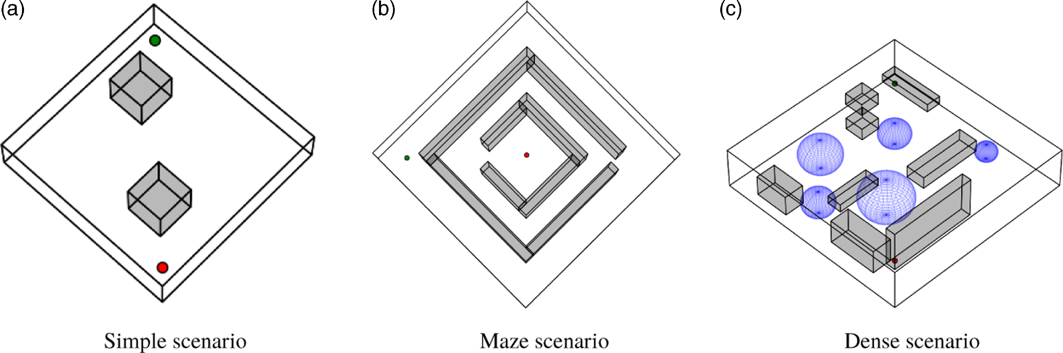
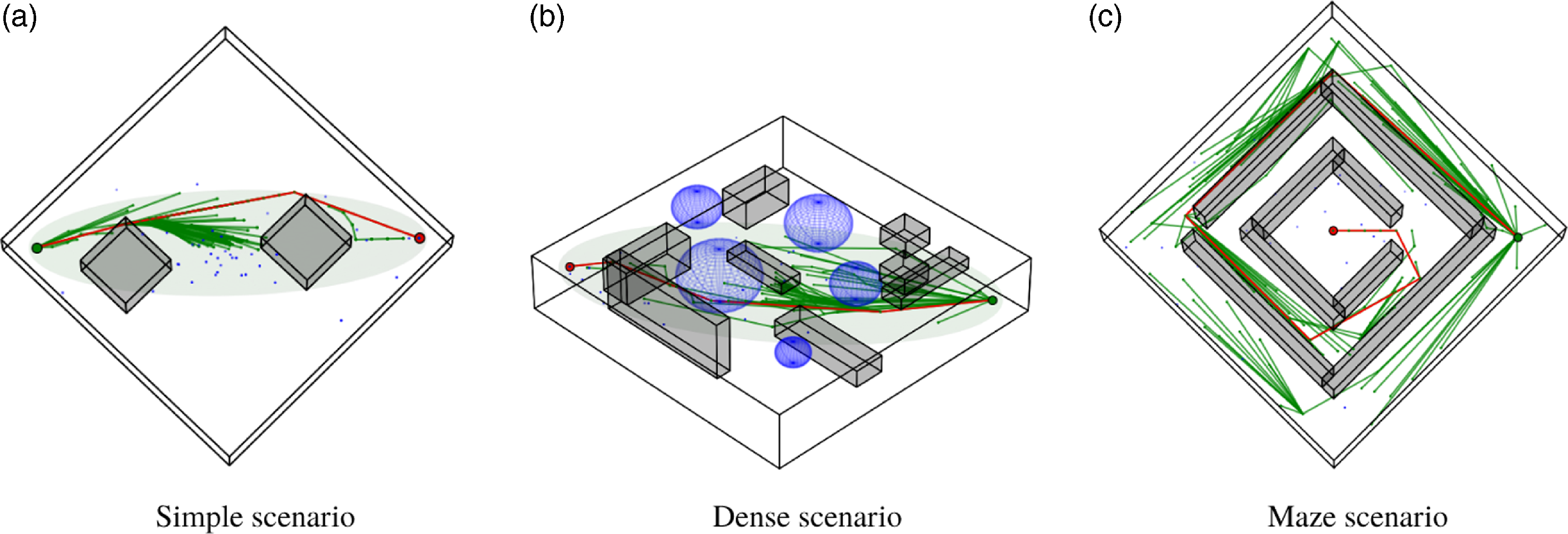
To evaluate the performance of the IBIT* algorithm, three typical 3-D scenarios were designed, as illustrated in Figure 4.
Three typical 3D scenarios.

The green and red points represent the start and end points, respectively, while the gray rectangular prisms, and blue spheres represent the obstacles. All scenarios share the dimensions of
 $20\times 20\times 5$
. In the simple scenario, there are only two primary obstacles, with the start and end points located at
 $\left ( \text{1}\text{.5, 1}\text{.5, 1} \right )$
and
 $\left ( \text{18}\text{.5, 18}\text{.5, 4} \right )$
, respectively. The maze scenario replicates a classic labyrinth, with the start and end points positioned at
 $\left ( \text{2, 2, 1} \right )$
and
 $\left ( \text{10, 10, 4} \right )$
[Reference Cui, Wang, Xiong, Mei and Wu31]. The dense scenario is filled with numerous closely packed obstacles and maintains the same start and end points as the simple scenario.
The first comparison validates the search time for the initial solution. Tests were conducted on a computer with an Intel(R) Xeon(R) Gold 6128 CPU @ 3.40 GHz and an NVIDIA Quadro P4000 GPU to measure the time taken for the BIT* and IBIT* algorithms to find initial solutions in typical scenarios. The initial solution search times for both algorithms are presented in Table I, with the data indicating that the IBIT* algorithm has a faster search speed for the initial solution compared to the BIT* algorithm, demonstrating a significant improvement.
Comparison of initial solution search time for paths in typical scenarios.

Important parameters of the four sampling path planning algorithms.

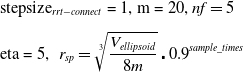
The IBIT* was compared with Improved Bi-P-RRT* [Reference Fan, Chen and Liang32], Informed-RRT*, and BIT*. These algorithms were tested repeatedly in three scenarios, with key parameter settings listed in Table II.
Figure 5 illustrates the average path lengths and execution times of the algorithms. The results demonstrate that the IBIT* algorithm significantly outperforms the other three algorithms in both initial solution search speed and solution convergence speed. In all three scenarios shown in Figure 5, IBIT* consistently achieves the earliest initial solution (indicated by the green curve starting farthest to the left on the time axis), validating the effectiveness of our proposed strategy for accelerating initial solution search. This strategy employs RRT-Connect, which exhibits rapid exploration capabilities.
Furthermore, Figure 5 shows that IBIT* achieves faster convergence (steep green curve decline) and shorter paths (lowest green curve). These improvements originate from: 1) Informed sparse sampling: Eliminating redundant sampling to enhance efficiency. 2) Parent node reselection: Pruning suboptimal branches, smoothing paths, and optimizing length.
Performance comparison curves of the four algorithms in typical scenarios.

In non-maze scenarios, IBIT* finds high-quality solutions within
 $20ms$
. Even in maze scenarios, it achieves solutions within
 $0.5s$
. Since maze-like scenarios rarely occur in practice, IBIT* proves ideal for online path planning in complex low-altitude environments.
4. Agile fixed-wing UAVs trajectory planning
4.1. Trajectory planning for multiple constraint conditions
In complex low-altitude environments, trajectory planning for agile fixed-wing UAVs faces numerous constraints. First, the presence of constricted flight corridors requires that aircraft adopt specific roll attitudes to navigate through them. Second, mission execution is subject to temporal constraints. Additionally, the kinematic properties of fixed-wing UAVs necessitate smooth trajectory generation. Lastly, the dynamic performance limitations of agile fixed-wing UAVs must also be considered. In summary, trajectory planning in such settings must account for constraints related to time, safety, UAV dynamic performance, and trajectory smoothness.
Conventional fixed-wing UAVs control lateral-directional movements through the combined use of ailerons and rudders to minimize sideslip. Due to the strong maneuverability and large control surfaces of agile fixed-wing UAVs, they can achieve lateral movement primarily using the rudder, with minimal influence from sideslip [Reference Ramírez and Nahon33]. Consequently, the ailerons of agile fixed-wing UAVs can be decoupled from controlling lateral-directional movement, treating the roll angle as an additional degree of freedom to enhance the survivability of agile fixed-wing UAVs in confined passageways. Based on this principle, the trajectory planning presented in this paper aims to optimize and solve for a state variable
 ${({{p}_{x}},{{p}_{y}},{{p}_{z}},\phi )}^{T}$
, which is composed of 3-D position and roll angle.
Since the IBIT* algorithm solely provides 3-D path points without incorporating roll angles, and the trajectory to be planned also includes roll angles, it is necessary to determine the initial roll angles corresponding to each 3-D path point generated by the IBIT* algorithm. In accordance with the lateral-directional dynamics of the UAV, the initial value of the roll angle can be written as
 \begin{equation} \phi =\arctan \frac {\overset {\centerdot }{\mathop {\psi }}\,{{V}_{a}}}{g}, \end{equation}
where
 ${V}_{a}$
,
 $\psi$
, and
 $g$
represent the airspeed, the yaw angle, and the gravitational acceleration, respectively. In trajectory planning, suboptimal initial roll angles at path points may result in insufficient roll angles in narrow corridors, risking collisions. However, given the typically short length of narrow corridors in complex low-altitude environments, unsafe roll angle sequences are limited. Thus, this issue is resolved during safety detection: if collision risk is detected, the roll angle is incrementally adjusted (by
 ${5}^{\circ }$
per step) until collision-free.
We have chosen MINCO for trajectory representation due to its capability to simultaneously optimize both time and space. MINCO inherently meets the condition of unconstrained minimum control efforts, which aligns with the requirement for trajectory smoothness. Moreover, MINCO can address the temporal constraints of mission time and the spatial constraints of safe flight corridors by leveraging its characteristics of spacetime deformation [Reference Wang, Zhou, Xu and Gao22].
UAV dynamic performance constraints primarily include speed and attitude angular velocity limitations. By representing trajectories with MINCO, smoothness is guaranteed, avoiding abrupt lateral/altitude position changes. Since pitch and yaw angles control longitudinal/lateral motion, their magnitudes and rates are indirectly constrained. Thus, only velocity and roll angle constraints are necessary for UAV dynamic performance.
We formulate the constraints in the form of soft constraints, which are incorporated into the objective function in the form of penalty function for optimization [Reference Bry, Richter, Bachrach and Roy23]. To facilitate program implementation, the i-th segment trajectory is discretized with a resolution of
 ${\kappa }_{i}$
. Therefore, the objective function for trajectory planning of an agile fixed-wing UAV in a complex low-altitude environment is
 \begin{equation} \begin{aligned} & \underset {\mathbf{c}(\mathbf{q},\mathbf{T})}{\mathop {\min }}\,J={{\lambda }_{V}}{{J}_{V}}+{{\lambda }_{\phi }}{{J}_{\phi }}+{{\lambda }_{{{\omega }_{\phi }}}}{{J}_{{{\omega }_{\phi }}}}+{{\lambda }_{{{\phi }_{la}}}}{{J}_{{{\phi }_{la}}}} \\[4pt] &s.t.\left \{ \begin{matrix} {{J}_{V}}=\sum \limits _{i=0}^{{{M}_{N}}}{\displaystyle\frac {{{T}_{i}}}{{{\kappa }_{i}}}\sum \limits _{j=0}^{{{\kappa }_{i}}}{K\left({{v}^{2}}\left({{t}_{i}},\displaystyle\frac {j}{{{\kappa }_{i}}}\right)-v_{\max }^{2}\right)+K\left(-{{v}^{2}}\left({{t}_{i}},\displaystyle\frac {j}{{{\kappa }_{i}}}\right)+v_{\min }^{2}\right)}} \\[12pt] {{J}_{\phi }}=\sum \limits _{i=0}^{{{M}_{N}}}{\displaystyle\frac {{{T}_{i}}}{{{\kappa }_{i}}}\sum \limits _{j=0}^{{{\kappa }_{i}}}{K\left({{\phi }^{2}}\left({{t}_{i}},\displaystyle\frac {j}{{{\kappa }_{i}}}\right)-\phi _{\max }^{2}\right)}} \\[12pt] {{J}_{{{\omega }_{\phi }}}}=\sum \limits _{i=0}^{{{M}_{N}}}{\displaystyle\frac {{{T}_{i}}}{{{\kappa }_{i}}}\sum \limits _{j=0}^{{{\kappa }_{i}}}{K\left(\omega _{\phi }^{2}\left({{t}_{i}},\displaystyle\frac {j}{{{\kappa }_{i}}}\right)-\omega {{_{\phi }^{2}}_{\max }}\right)}} \\[12pt] {{J}_{{{\phi }_{la}}}}=\sum \limits _{i=0}^{{{M}_{N}}}{\displaystyle\frac {{{T}_{i}}}{{{\kappa }_{i}}}\sum \limits _{j=0}^{{{\kappa }_{i}}}{K\left(-\phi \left({{t}_{i}},\displaystyle\frac {j}{{{\kappa }_{i}}}\right)\overset {\centerdot }{\mathop {\psi \left({{t}_{i}},\frac {j}{{{\kappa }_{i}}}\right)}}\,\right)}} \\[8pt] \end{matrix} \right . \\ \end{aligned}, \end{equation}
where
 ${M}_{N}$
is the number of trajectory points;
 ${{v}_{\max }},{{v}_{\min }}$
,
 ${\phi }_{\max }$
, and
 ${\omega }_{{{\phi }_{\max }}}$
are the lower and upper bounds of the UAV velocity, the maximum roll angle, and the maximum roll rate, respectively;
 ${{\lambda }_{V}},{{\lambda }_{\phi }},{{\lambda }_{{{\omega }_{\phi }}}},{{\lambda }_{{{\phi }_{la}}}}$
is the weight corresponding to the penalty term; and
 ${T}_{i}$
stands for the time of the i-th trajectory.
Maximum speed penalty
 ${J}_{V}$
: Fixed-wing UAV have a minimum flight speed
 ${v}_{min}$
and a maximum flight speed
 ${v}_{max}$
, and thus
 ${J}_{V}$
addresses the constraints from both aspects.
Maximum roll angle penalty
 ${J}_{\phi }$
: The UAV’s roll angle has a range of
 $[\begin{matrix} 0 & \pm {{180}^{{}^\circ }} \\ \end{matrix}]$
.
Maximum roll rate penalty
 ${J}_{{{\omega }_{\phi }}}$
: The UAV’s roll rate is limited to a maximum roll rate of
 ${\omega }_{{{\phi }_{\max }}}$
.
Roll angle direction penalty
 ${J}_{{{\phi }_{la}}}$
: This describes the constraints on the roll angle direction of the UAV. The lateral forces acting on a fixed-wing UAV are generated by the deflection of both the rudder and the ailerons [Reference Lu, Li and Xu34]. To improve flight stability, it is typically expected that the yaw rate resulting from rudder deflection aligns with the roll angle produced by aileron deflection.
The penalty function for the roll angle direction constraint can be designed as follows:
 \begin{equation} \begin{matrix} {{\tau }_{la}}=K({-}\phi \overset {\centerdot }{\mathop {\psi }}\,) & \overset {\centerdot }{\mathop {{{\tau }_{la}}}}\,=-\overset {\centerdot }{\mathop {K}}\,(-\phi \overset {\centerdot }{\mathop {\psi }}\,)\centerdot (\overset {\centerdot }{\mathop {\phi }}\,\overset {\centerdot }{\mathop {\psi }}\,+\phi \overset {\centerdot \centerdot }{\mathop {\psi }}\,) \\ \end{matrix}. \end{equation}
The expected yaw angle on the trajectory and its first and second derivatives are as follows:
 \begin{equation} \begin{matrix} \psi =-\arctan \left(\displaystyle\frac {{{v}_{y}}}{{{v}_{x}}}\right),\text{ }\overset {\centerdot }{\mathop {\psi }}\,=\displaystyle\frac {{{a}_{x}}{{v}_{y}}-{{a}_{y}}{{v}_{x}}}{{{v}_{x}}^{2}+{{v}_{y}}^{2}} \\[10pt] \overset {\centerdot \centerdot }{\mathop {\psi }}\,=\displaystyle\frac {\left ( jer{{k}_{x}}{{v}_{y}}-jer{{k}_{y}}{{v}_{x}} \right )\left ( {{v}_{x}}^{2}+{{v}_{y}}^{2} \right )-2\left ( {{a}_{x}}{{v}_{x}}+{{a}_{y}}{{v}_{y}} \right )\left ( {{a}_{x}}{{v}_{y}}-{{a}_{y}}{{v}_{x}} \right )}{{{\left ( {{v}_{x}}^{2}+{{v}_{y}}^{2} \right )}^{2}}} \\ \end{matrix}. \end{equation}
The state variables of the UAV, such as
 $v,{{v}_{x}},{{a}_{x}},jer{{k}_{x}},\overset {\centerdot }{\mathop {\phi }}\,$
, can be represented using four independent state variables
 $z={{({{p}_{x}},{{p}_{y}},{{p}_{z}},\phi )}^{T}}$
and their respective derivatives. When the directions of the roll angle and yaw rate are the same, there is
 $-\phi \overset {\centerdot }{\mathop {\psi }}\,\lt 0,F(-\phi \overset {\centerdot }{\mathop {\psi }}\,)\lt 0$
; when the signs of the roll angle and yaw rate differ, there is
 $-\phi \overset {\centerdot }{\mathop {\psi }}\,\gt 0,F(-\phi \overset {\centerdot }{\mathop {\psi }}\,)\gt 0$
, which can constrain the direction of the roll angle. The expressions for function
 $K(\cdot )$
and its derivatives are as follows:
 \begin{equation} \begin{matrix} K(x)=\left \{ \begin{matrix} 0 &\quad x\lt 0 \\[6pt] \displaystyle\frac {2{{\mu }_{x}}{{x}^{3}}-{{x}^{4}}}{2{{\mu }_{x}}^{3}} &\quad 0\leq x\leq {{\mu }_{x}} \\[6pt] x- \displaystyle\frac {1}{2}{{\mu }_{x}} &\quad x\gt {{\mu }_{x}} \\[6pt] \end{matrix} \right . &\quad \displaystyle\frac {dK(x)}{dx}=\left \{ \begin{matrix} 0 &\quad x\lt 0 \\[6pt] \displaystyle\frac {3{{\mu }_{x}}{{x}^{2}}-2{{x}^{3}}}{{{\mu }_{x}}^{3}} &\quad 0\leq x\leq {{\mu }_{x}} \\[6pt] 1 & x\gt {{\mu }_{x}} \\ \end{matrix} \right . \\ \end{matrix}, \end{equation}
where
 ${\mu }_{x}$
is a range related to dynamic performance
 $x$
, enabling approach to state limits. Parameters can vary with performance needs. The piecewise function
 $K(\centerdot )$
is continuous and differentiable at segment points. It effectively constrains dynamic performance and acts as a penalty function.
By combining the gradient of the objective function with respect to the control variable and the time, along with the gradients of the penalties in Equation (6), we can obtain the complete gradient expression [Reference Wang, Zhou, Xu and Gao22]. Finally, numerical optimization can be carried out using the gradient descent method.
4.2. Trajectory planning experiments for agile fixed-wing UAV in complex low-altitude environment
Path planning of the IBIT* in typical scenarios.

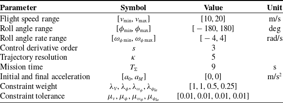
Trajectory planning constraints and experimental parameter settings.

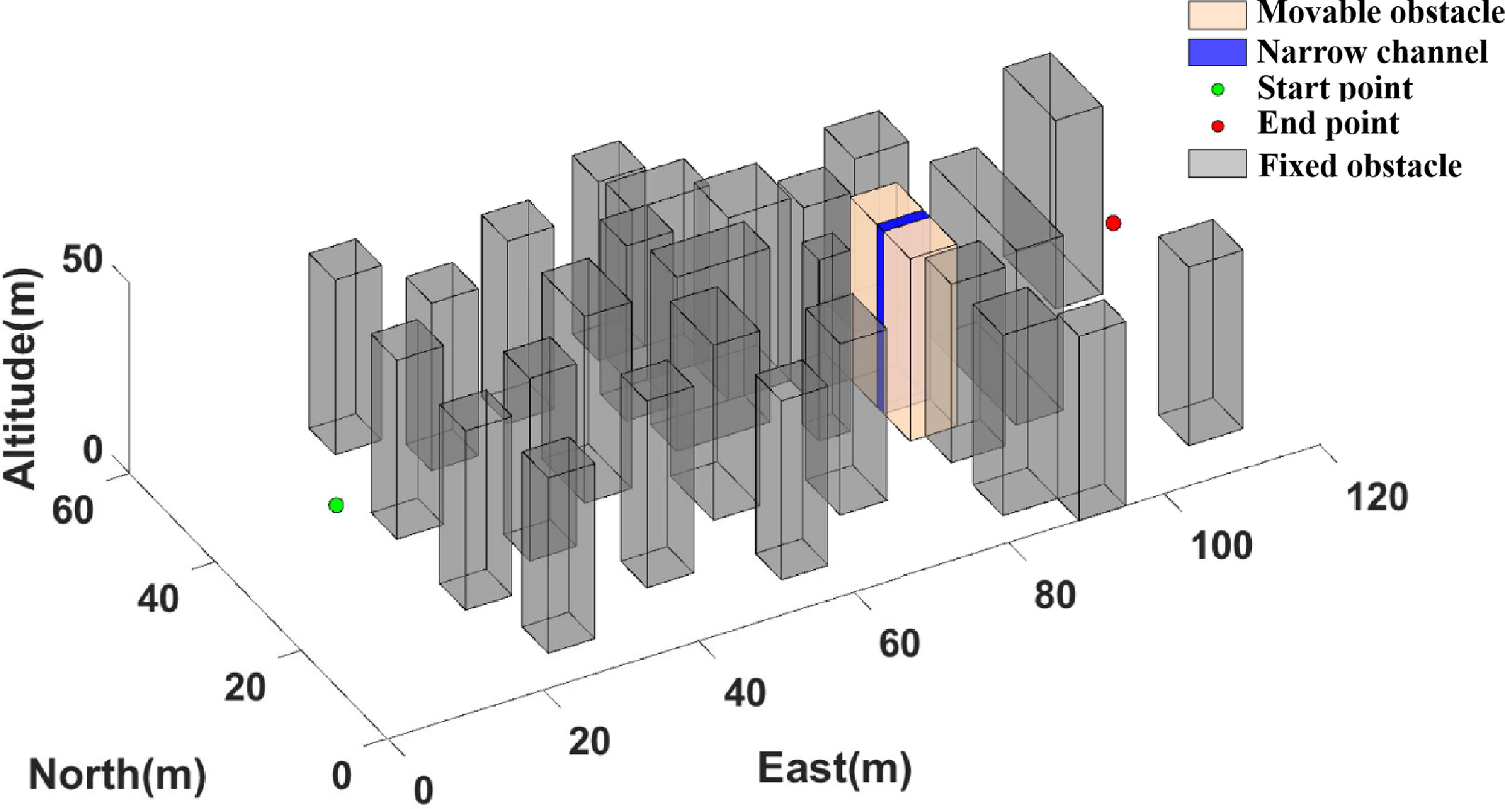
Typical complex low-altitude environment.

Figure 7 shows a complex low-altitude environment with a narrow corridor, whose width can be adjusted to test trajectory planning in narrow spaces. Experimental parameters are shown in Table III.
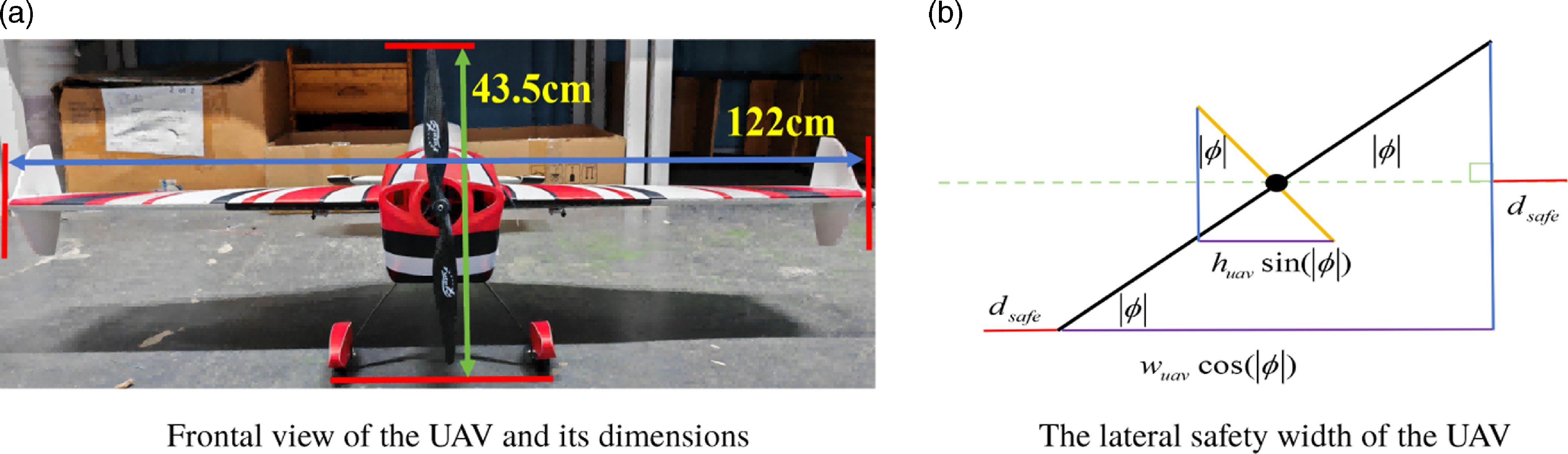
Considering the ability of the small agile fixed-wing UAV, we use to fly safely in complex low-altitude environments, it is important to recognize that the UAV is a physical object with specific dimensions and should not be treated as a mass. In order to navigate safely through narrow corridors, it is necessary to model a safe width for a small agile fixed-wing UAV. A frontal view and safe width schematic of this UAV is shown in Figure 8, where the height of the vehicle is
 ${{h}_{uav}}=43.5cm$
and the width is
 ${{w}_{uav}}=122cm$
when all three-axis attitude angles are set to zero.
To ensure sufficient flight safety, a lateral safety distance
 ${{d}_{safe}}=50cm$
is specified, and the relationship between the UAV’s safety width
 ${w}_{ef}$
and the aircraft’s roll angle
 $\phi$
is given by Equation (10).
 \begin{equation} {{w}_{ef}}=\left \{ \begin{matrix} {{h}_{uav}}\sin (\left | \phi \right |)+2{{d}_{safe}} &\quad \left | \phi \right |\in \left [ \begin{matrix} {{70.376}^{\circ }} &\quad {{109.624}^{\circ }} \\ \end{matrix} \right ] \\[8pt] {{w}_{uav}}\cos (\left | \phi \right |)+2{{d}_{safe}} &\quad otherwise \\ \end{matrix} \right ., \end{equation}
Frontal view and safety width diagram of small agile fixed-wing UAV.

Trajectory planning in the narrow corridor.

The UAV requires a maximum safe width of
 ${{w}_{ef\_\max }}=2.22m$
when
 $|\phi |=k\pi \ (k=0,1)$
, and a minimum width of
 ${{w}_{ef\_\min }}=1.4m$
when
 $\left | \phi \right |={{70.376}^{\circ }}$
or
 $\left | \phi \right |={{109.624}^{\circ }}$
. These widths correspond to
 $1.82$
and
 $1.15$
times the wingspan of the UAV, respectively.
4.2.1 Experiment with a narrow corridor width of
 $1.82$
times the wingspan

The narrow corridor is
 $2.22m$
wide, with initial/final velocities of
 $15m/s$
and roll angles of
 ${0}^{\circ }$
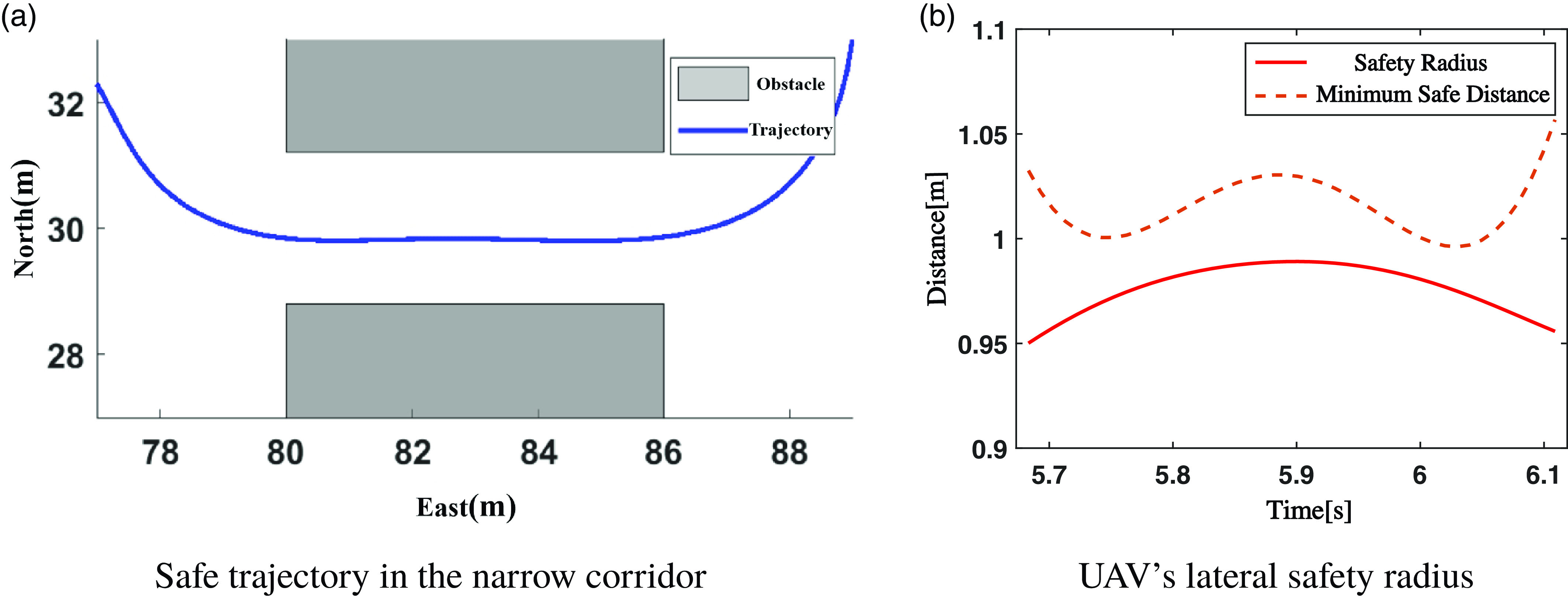
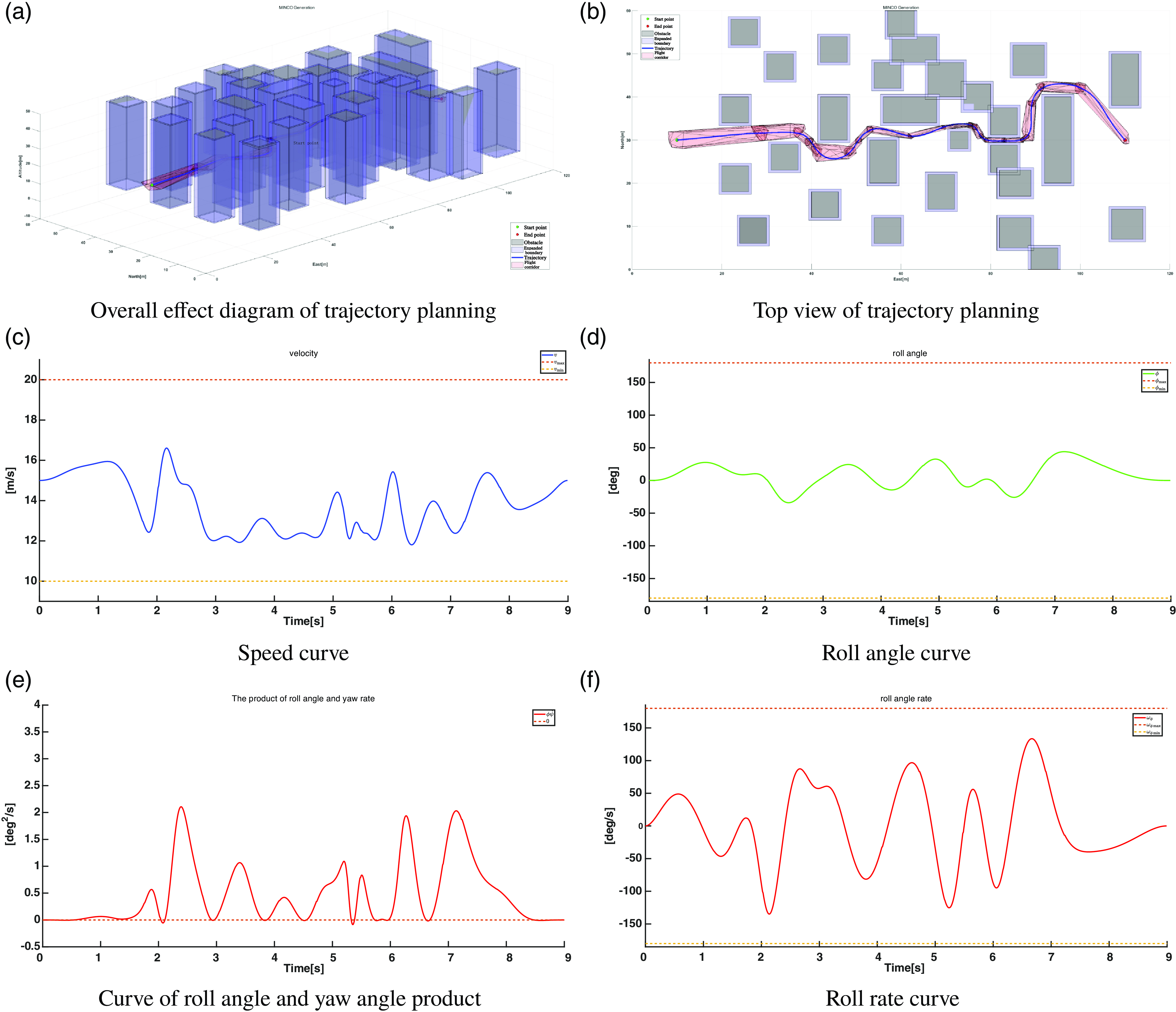
. Trajectory planning under these conditions generates a constraint-satisfying trajectory (Figure 10) with
 $71.8ms$
computation time. The trajectory in the narrow corridor, along with the UAV’s lateral safety radius and the minimum safe distance to obstacles, is shown in Figure 9. In this segment of the trajectory, the UAV’s lateral safety radius always remains smaller than the minimum safe distance from the obstacles.
4.2.2 Experiment with a narrow corridor width of
$1.15$
times the wingspan

The width of the narrow corridor is set to
 $1.4m$
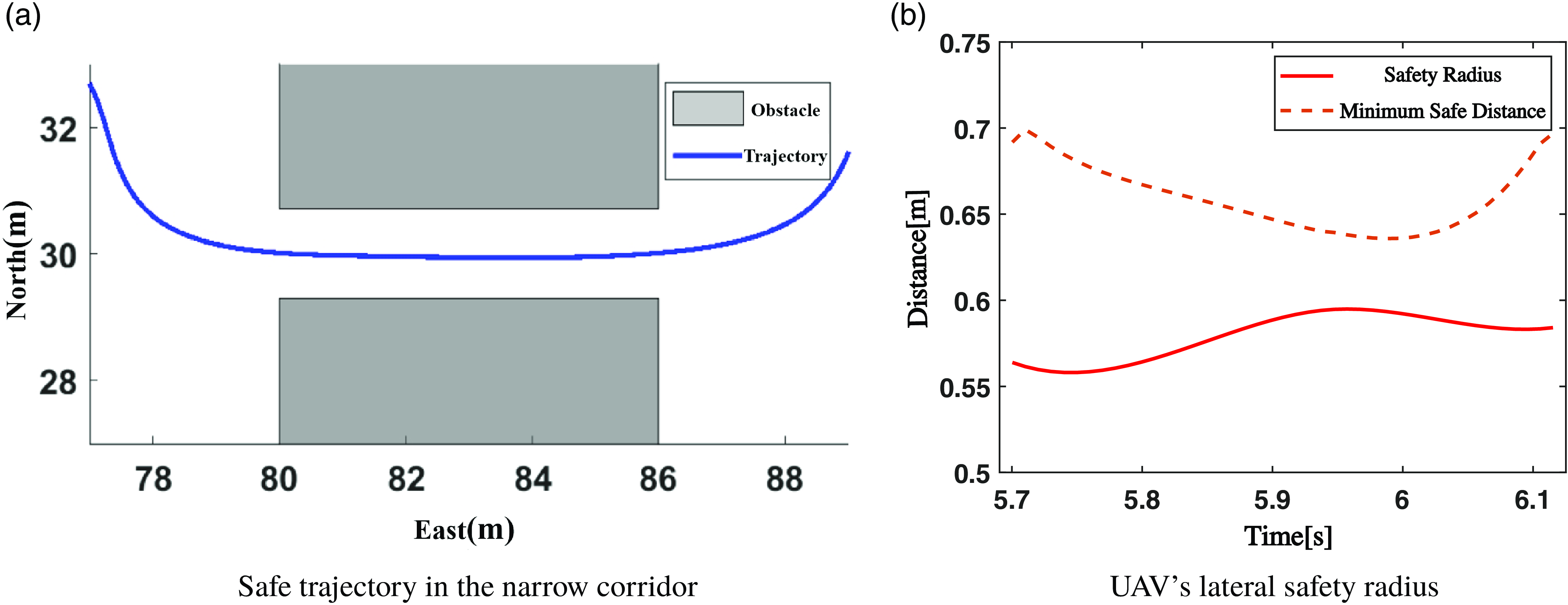
, and the initial conditions are the same as those in the previous experiment. Under these initial conditions, the trajectory planning results are shown in Figure 12. The algorithm took only
 $67.6ms$
, and the planned trajectory is smooth, remaining entirely within the SFC. The velocity, roll angle, roll rate, and other parameters of the trajectory all satisfy the constraints.
Trajectory planning for a narrow corridor width of
 $1.82$
times the wingspan.

Trajectory planning in the narrow corridor.

Trajectory planning for a narrow corridor width of
 $1.15$
times the wingspan.

Figure 11 shows the UAV trajectory through the
 $1.15$
times wingspan narrow corridor and the minimum safe distance curve. The smooth trajectory maintains safe lateral distances from obstacles. Throughout the passage, the lateral safety radius remains below the minimum distance, confirming safe navigation with proper roll angles.
In typical scenarios, the algorithm for trajectory planning can be controlled to within
 $100ms$
. Considering that motion planning involves steps such as path planning and the construction of a SFC, our single motion planning can still be maintained around
 $200ms$
, which meets the requirements for online planning.
Furthermore, it is important to note that the trajectory planning method we proposed is the first to introduce MINCO to agile fixed-wing UAV, enabling planning with roll angles. We have also designed a penalty function for soft constraint numerical optimization. Our trajectory planning aims to achieve higher solution efficiency while satisfying constraints. Given that numerical optimization methods already demonstrate higher efficiency compared to other optimization approaches, and that MINCO exhibit greater efficiency than other trajectory representations, such as B-spline, it can be concluded that our proposed trajectory planning method offers distinct advantages.
5. Physical flight test in a virtual complex low-altitude environment
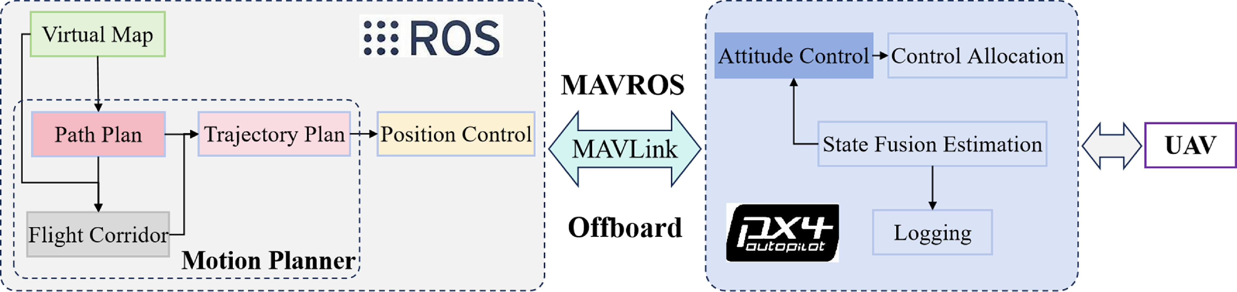
We control the agile fixed-wing UAV using ROS and PX4, with MAVROS enabling data transmission and acquisition. Figure 13 illustrates our designed autonomous flight software framework. The left side of the figure, implemented on the upper computer, adopts the trajectory tracking strategy from [Reference Ramírez and Nahon29]. While real low-altitude environments require perception sensors for local data, we employ virtual environmental perception due to construction challenges and our non-focus on perception/mapping. For instance, we simulate a
 $20m$
-radius detection range using a virtual lidar, assuming the UAV acquires environmental data within this scope.
Flight system software framework.

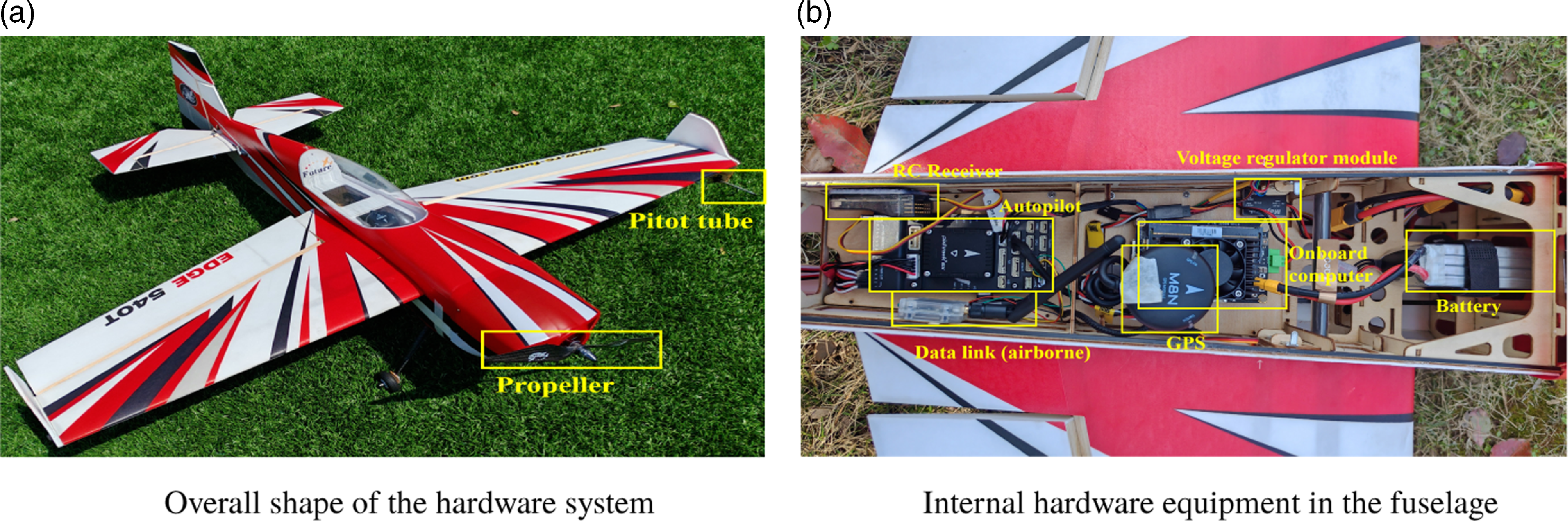
The hardware system (Figure 14) features an EDGE-540T-30E-based UAV measuring
 $1.21m$
length,
 $1.22m$
wingspan,
 $30d{{m}^{2}}$
wing area, and
 $1.52Kg$
total mass. Constructed from lightweight yet strong PP material, its three control surfaces achieve
 ${50}^{\circ }$
maximum deflection for exceptional roll/lateral performance. The platform integrates a Pixhawk-6X flight controller, Jetson Xavier NX computer, enhanced-torque TMOTOR AM480-KV900 motors (2:1 thrust-to-weight ratio), and GDW DS296X digital servos for rapid deflection response.
Small agile fixed-wing UAV test platform.

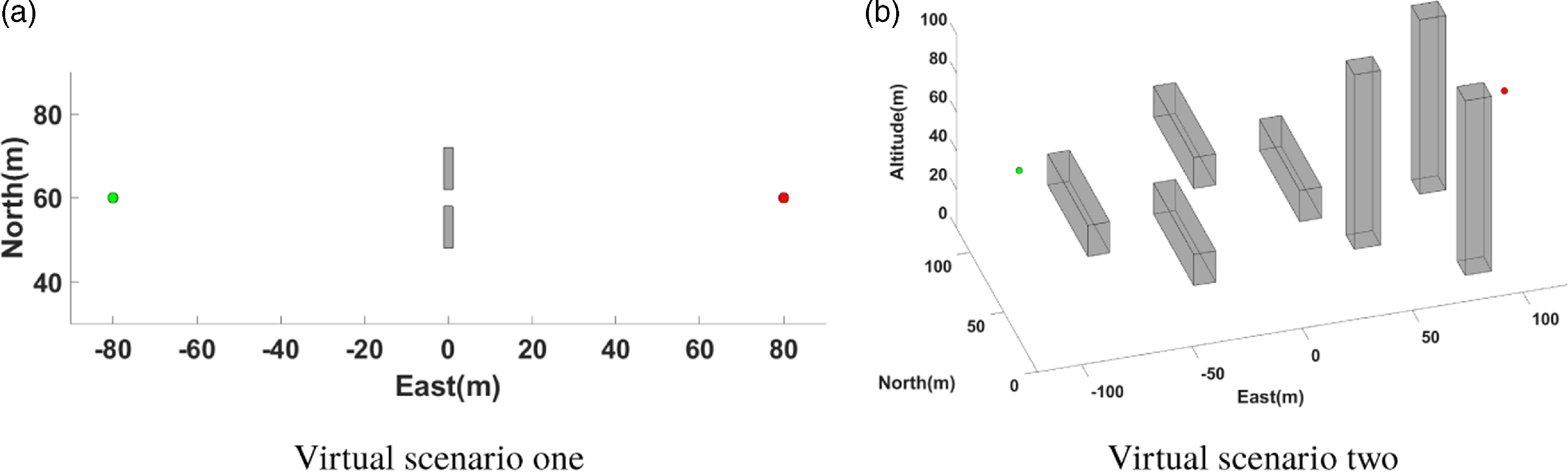
To validate the effectiveness of the motion planning algorithm for agile fixed-wing UAVs in complex low-altitude environments, two virtual scenarios are created. Scenario one tests whether the UAV can safely traverse a
 $5m$
-wide narrow corridor, while scenario two assesses obstacle avoidance capabilities in environments with both vertical and horizontal obstacles. Figure 15 illustrates these scenarios.
Virtual scenario for flight experiments.

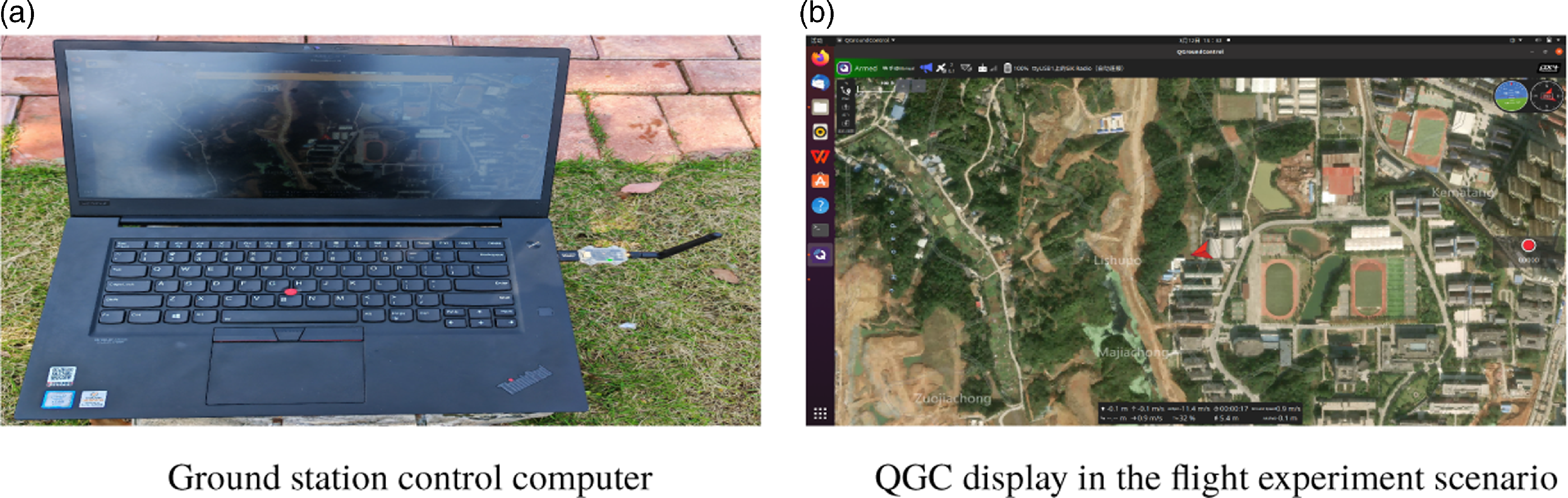
Figure 16 shows the experimental setup with ground control computer and QGroundControl (QGC) interface. The computer connects to the ground station for real-time UAV status monitoring via QGC. Pre-flight procedures include sensor calibration (accelerometer, magnetometer, level, and airspeed) and configuring the remote controller’s mode/safety switches until QGC confirms green arm status.
Ground station computer and QGC display screen.

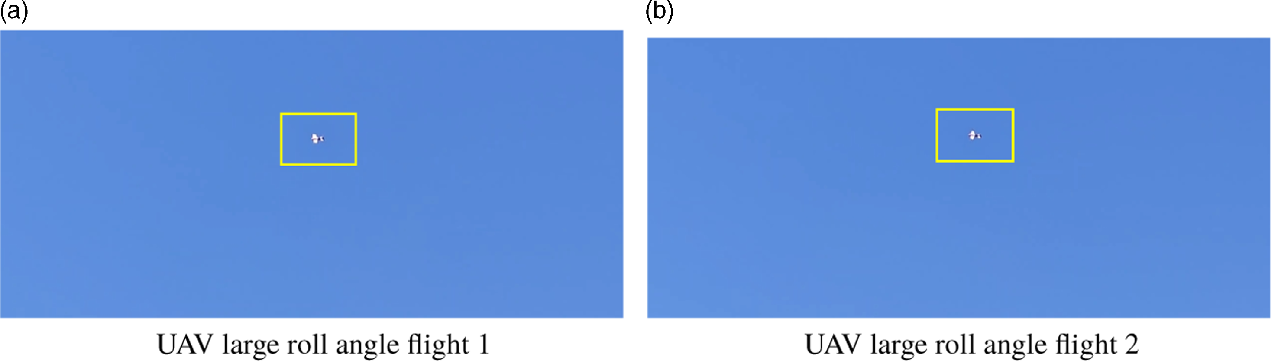
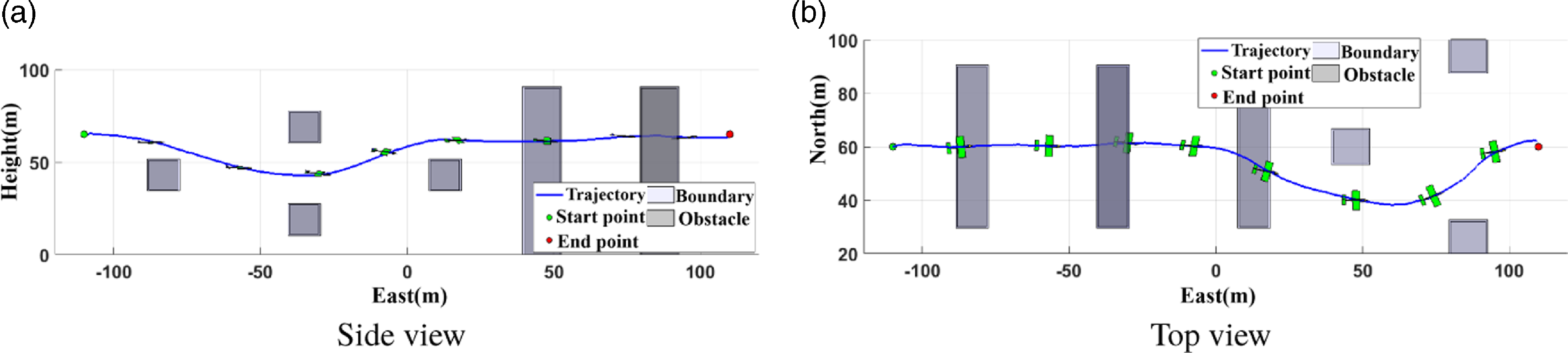
The process of conducting flight experiments in virtual scenario one is illustrated in Figure 17, where the agile fixed-wing UAV maneuvers through a narrow corridor with a significant roll angle.
Images from the flight experiment process in virtual scenario 1.

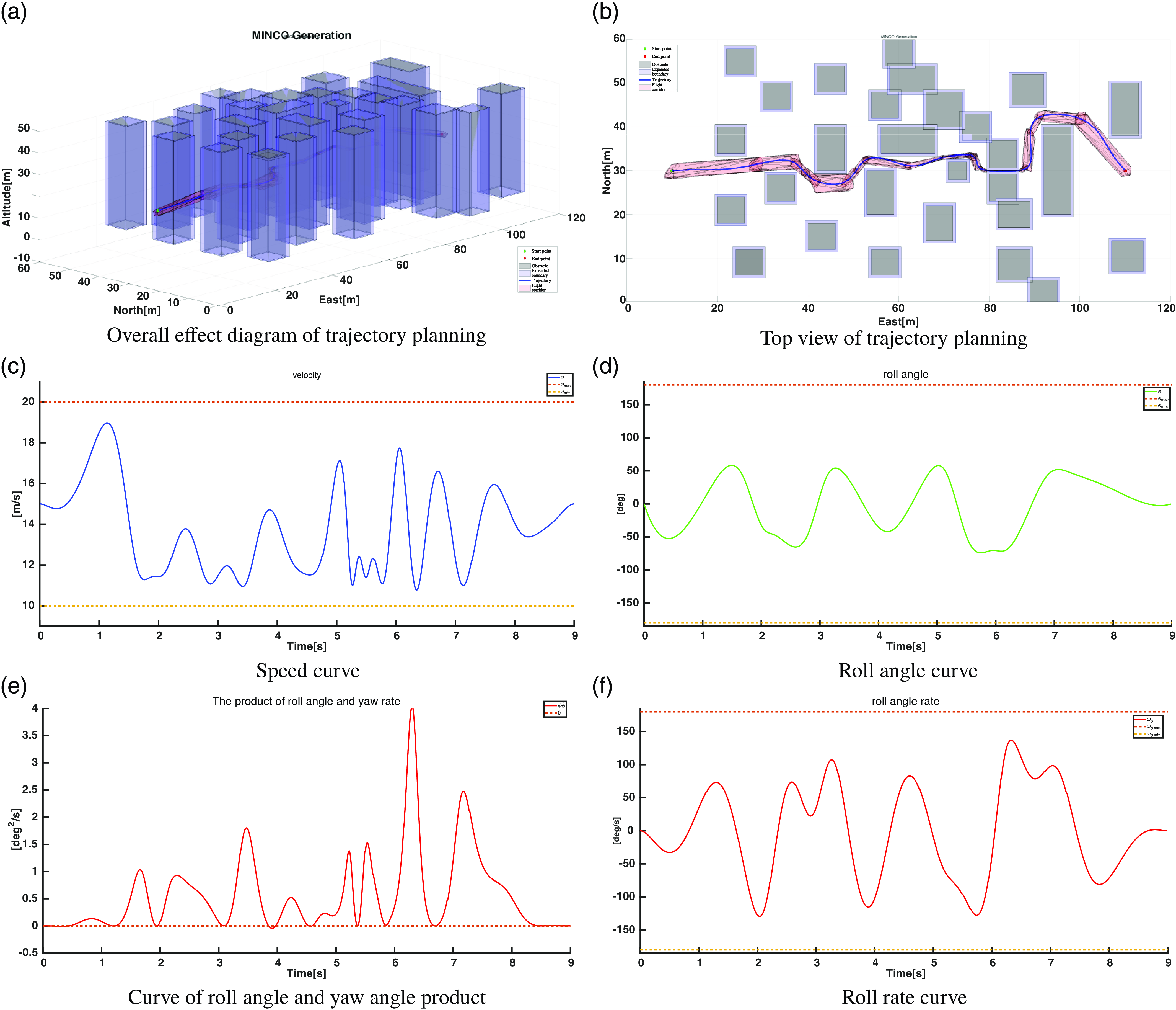
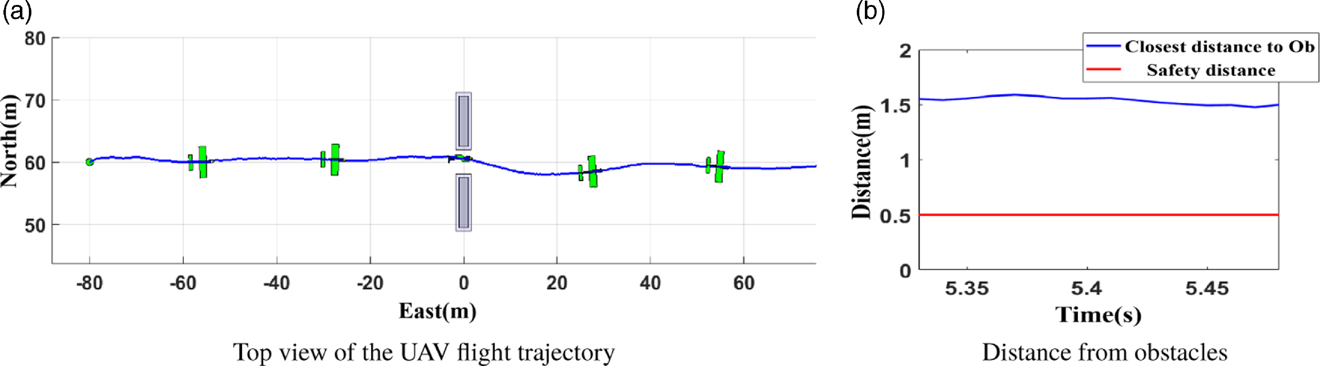
Figure 18 presents the experimental results in virtual scenario one, where the closest distance between the UAV and the obstacle while passing through the narrow corridor is always greater than the safety distance, indicating that the UAV safely traverses the narrow corridor formed by the obstacles.
Experimental results in virtual scenario 1.

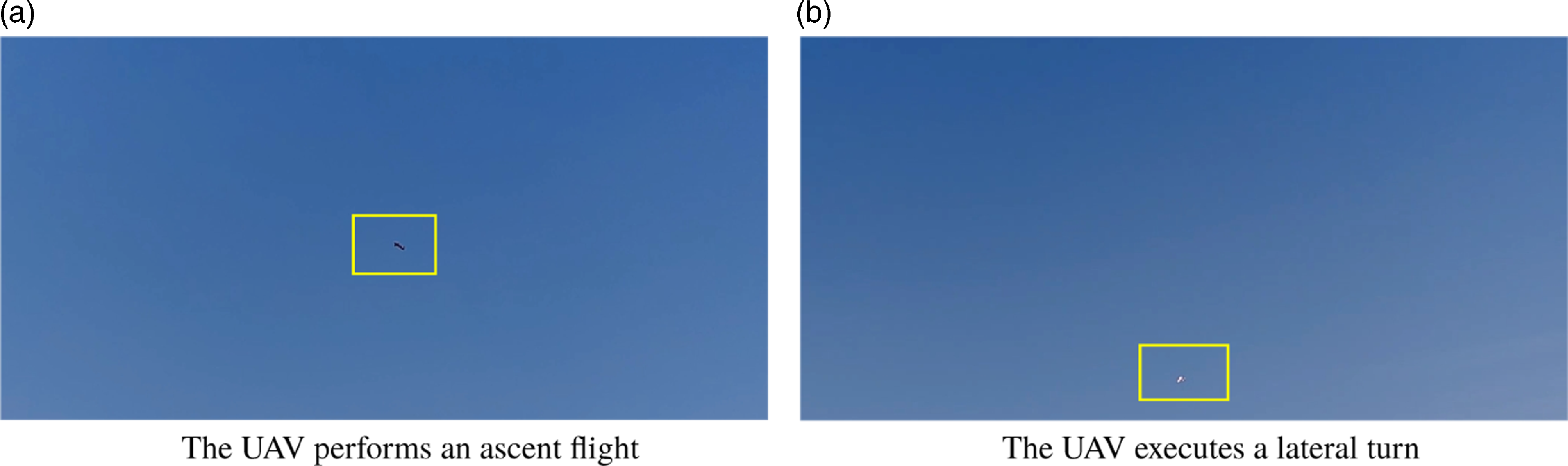
Flight experiments in Virtual Scenario 2 are shown in Figure 19, illustrating the ascent and lateral turning flights of the agile fixed-wing UAV to avoid obstacles.
Images from the flight experiment process in virtual scenario 2.

In Figure 20, the UAV’s flight in Virtual Scenario 2 shows that the distance between the UAV and the obstacles is significantly greater than the safety distance, allowing the UAV to safely traverse the narrow corridor created by the obstacles.
Experimental results in virtual scenario 2.

6. Conclusion and future works
This paper investigates the motion planning problem for agile fixed-wing UAV in complex low-altitude environment. In the path planning layer, we propose the IBIT*, which has been verified in typical scenarios to improve both the quality of the planned path and the computation speed. In the trajectory planning layer, we decouple the UAV’s roll angle from its 3-D position, eliminate the spatial and temporal constraints of the flight corridor, and design a penalty function based on the dynamic performance constraints of the UAV. Experiments conducted in typical scenarios demonstrate the effectiveness of the trajectory planning. Finally, we built a physical flight system for a small agile fixed-wing UAV, which safely navigated in a complex low-altitude environment during practical experiments, validating the effectiveness of our proposed methods.
Although we have achieved safe flight for the agile fixed-wing UAV in complex low-altitude environments, there are still some issues that need to be addressed in the future. We can explore environmental perception methods suitable for fixed-wing UAVs in complex low-altitude environments, particularly by equipping small visual or laser sensors to enable real-time state estimation on board, helping the UAV accurately determine its pose information. Additionally, we can continue to develop the maneuverability of agile fixed-wing UAVs, which have the potential for stall flight at high angles of attack.
Author contributions
F. Zou conceived, designed, and completed the research and writing of the paper; J. Li participated in the design of the research ideas; Y. Niu provided the overall writing strategy for the paper and support for the flight experiments.
Financial support
This work was supported by the National Natural Science Foundation of China under Grant 61876187.
Conflicts of interest
The authors declare no conflicts of interest exist.
Ethical approval
Not applicable.