Introduction
Mountains encompass a variety of suitable habitats for numerous species with different ecological requirements (Körner Reference Körner2004, Salas-Morales & Meave Reference Salas-Morales and Meave2012, Sundqvist et al. Reference Sundqvist, Giesler and Wardle2011), thus they have been considered biodiversity hotspots worldwide (Boulangeat et al. Reference Boulangeat, Lavergne, Garraud and Thuiller2012, Lomolino Reference Lomolino2001, Neri et al. Reference Neri, Borges, Meira-Neto, Magnago, Trotter, Schaefer and Porembski2016). In particular, altitude-related changes in soil fertility and soil texture act as important environmental filters determining variation in plant populations (Neri et al. Reference Neri, Borges, Meira-Neto, Magnago, Trotter, Schaefer and Porembski2016, Urbanetz et al. Reference Urbanetz, Lehn, Salis, Bueno and Alves2012). Ultimately, such filtering causes niche displacement or partitioning (Bertoncello et al. Reference Bertoncello, Yamamoto, Meireles and Shepherd2011, Laliberté et al. Reference Laliberté, Zemunik and Turner2014, Maragon et al. Reference Maragon, Soares, Feliciano, Lani and Matos2013, Schaefer et al. Reference Schaefer, Amaral, Mendonça, Oliveira, Lani, Costa and Fernandes-Filho2008), which is reflected as a strong species turnover along the gradient (Eisenlohr et al. Reference Eisenlohr, Alves, Bernacci, Padgurschi, Torres, Prata, dos Santos, Assis, Ramos, Rochelle, Martins, Campos, Pedroni, Capel-Sanchez, Pereira, Vieira, Gomes, Tamashiro, Scaranello, Caron and Joly2013, Rodrigues et al. Reference Rodrigues, Schaefer, Silva, Ferreira-Júnior, Santos and Neri2018). For example, the gravity-driven nutrient transport downslope results in higher soil fertility at the lowest altitudes, which promotes the presence there of some species while excluding some others (Martins et al. Reference Martins, Silva, de Souza and Neto2003, Souza et al. Reference Souza, Lelis, Schaefer, Souza and Meira-Neto2012). Thus, altitudinal gradients can be regarded as heterogeneous systems, across which a broad array of ecological factors regulates species richness and diversity patterns (Born et al. Reference Born, Pluess, Burslem, Nilus, Maycock and Ghazoul2014, Körner Reference Körner2004, Méndez-Toribio et al. Reference Méndez-Toribio, Meave, Zermeño-Hernández and Ibarra-Manríquez2016).
In the semi-arid region of Brazil, known as Caatinga, mountain ranges of Tertiary age and reaching altitudes up to 1000 m presently occur as isolated areas amid the surrounding plateau. Although the Caatinga comprises a complex mosaic of plant communities, the vegetation is mainly characterized by the dominance of relatively short trees, usually shorter than 10 m, along with many species of shrubs and cacti (Moro et al. Reference Moro, Silva, Araújo, Lughadha, Meagher and Martins2015, Silva & Souza et al. Reference Silva and Souza2018). This region is marked by strong climatic seasonality in water availability, in response to which plants have evolved a set of particular morphological and functional adaptations, including the presence of thorns, leaf deciduousness, small leaves, and stem and root succulence (Prado Reference Prado2003, Queiroz et al. Reference Queiroz, Cardoso, Fernandes, Moro, da Silva, Leal and Tabarelli2017, Silva & Souza Reference Silva and Souza2018). At local scales, however, other environmental variables such as topography, terrain slope, soil moisture and anthropic disturbance also play key roles in community assembly in these ecosystems (Rezende et al. Reference Rezende, Miranda, Meyer, Moreira, Linhares, Oliveira-Filho and Eisenlohr2015, Ribeiro et al. Reference Ribeiro, Santos, Arroyo-Rodríguez, Tabarelli, Souza and Leal2016, Rito et al. Reference Rito, Arroyo-Rodríguez, Queiroz, Leal and Tabarelli2017 a, Silva & Souza Reference Silva and Souza2018).
Studies in the mountain ranges of Brazil’s semi-arid region have revealed a distinct pattern of plant distribution, characterized by increasing species richness towards higher altitudes (Almeida et al. Reference Almeida, Ramos, Diniz and Lopes2020, Lopes et al. Reference Lopes, Ramos and Almeida2017, Silva et al. Reference Silva, Lopes, Lopez, Melo and Trovão2014). The causes of this pattern are unclear; for one, they could be related to the role of mountains as natural barriers that hamper human access, and to more humid climates than in surrounding areas, all of which may favour a higher diversity (Lopes et al. Reference Lopes, Ramos and Almeida2017, Silva et al. Reference Silva, Lopes, Lopez, Melo and Trovão2014). However, this pattern could also be associated with edaphic factors, but their influence on plant community assembly in these systems is yet to be assessed. In addition to the effects of altitude-related gradients, such as temperature and air moisture (Salas-Morales et al. Reference Salas-Morales, Meave and Trejo2015), edaphic variables along them may increase environmental complexity and heterogeneity, thus favouring the persistence of different floristic and structural arrays (Andersen et al. Reference Andersen, Corre, Turner and Dalling2010, Barros et al. Reference Barros, Pinho, Leão and Tabarelli2017, Foster et al. Reference Foster, Questad, Collins, Murphy, Dickson and Smith2011).
The objective of this study was to analyse the role of edaphic variables on plant species richness and diversity along altitudinal gradients in the Brazilian semi-arid region. First, we hypothesized that the different micro-habitats that occur along the gradients derived from nutrient transport from the mountain top to its base enhance the altitudinal variability of vegetation structure and species composition. We further hypothesized that the low species diversity at the mountain foothills is associated with the high fertility typical of those areas, as a result of resource monopolization by a few species.
Methods
Study area
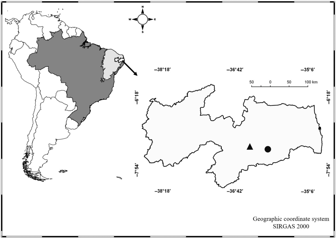
The study was carried out on two mountain ranges, namely Serra de Bodocongó, which attains an altitude of 680 m asl (hereafter S1; 7°27′6′′S, 35°59′41′′W), and Serra da Arara, whose maximum altitude is 660 m asl (hereafter S2; 07°23′8.1′′S, 36°23′36.7′′W) (Figure 1), both located in the Planalto (Plateau) da Borborema, Paraíba state, north-eastern Brazil. Altitude at the plateau ranges mostly between 150–650 m asl, with isolated peaks such as Pico do Jabre reaching altitudes as high as 1100 m asl (Velloso et al. Reference Velloso, Sampaio and Pareyn2002).
Geographic location of the study sites on the Borborema Plateau, Paraíba state, north-eastern Brazil. S1 (circle), Bodocongó mountain; S2 (triangle), Arara mountain.

In this region the prevailing climate is Bswh’ (warm semi-arid), according to the updated Köeppen–Geiger climate classification (Álvares et al. Reference Álvares, Stape, Sentelhas, de Moraes Gonçalves and Sparovek2013). Average total annual precipitation is fairly low, ranging from 350–650 mm year−1. Mean annual temperature varies between 25°C and 41°C. Two well-marked seasons are distinguished, one dry (August–February) and one humid (March–July) (Velloso et al. Reference Velloso, Sampaio and Pareyn2002). These climatic features result in low and irregular water availability in the region, which is the main driver of vegetation structure and composition (Silva & Souza Reference Silva and Souza2018).
The semi-arid Brazilian Caatinga comprises two contrasting geological domains, namely a crystalline domain and a sedimentary domain (Ab’ Sáber Reference Ab’ Sáber1974). The sedimentary domain is clearly more humid, with better-developed soils and the presence of dry forests with bigger trees; moreover, precipitation is higher in some areas of this domain, favouring the presence of patches of humid and sub-humid vegetation surrounded by the seasonally dry tropical forest (Silva & Souza Reference Silva and Souza2018). Specifically, this study was conducted in the crystalline domain, which is characterized by shallow, rocky and nutrient-rich soils. The prevailing soils in the study area probably qualify as Chromic Luvisols, according to World Reference Base for soil resource (IUSS Working Group WRB 2014). Erosive processes in the Tertiary exposed the region’s Precambrian granitic and gneissic basement (Ab’ Sáber Reference Ab’ Sáber1974), while some places where the bedrock was more resistant remained as higher, isolated areas with a distinct vegetation structure and composition, somewhat resembling the vegetation of more humid environments such as the Atlantic Forest (Silva & Souza Reference Silva and Souza2018). For these reasons, the seasonally dry tropical forest domain of Brazil is characterized by a large environmental heterogeneity (Moro et al. Reference Moro, Lughadha, Araújo and Martins2016).
The region around the mountains encompasses an array of dry forest fragments created by extensive farming. These fragments are marked by the presence of trails left by grazing animals and local inhabitants collecting forest resources. Vegetation of these fragments is dominated by shrubs and short-statured trees with xeromorphic adaptations (Prado Reference Prado2003), including species such as Croton blanchetianus and Cenostigma pyramidale. Between intermediate altitudes and the mountains’ upper reaches vegetation is better developed and species diversity is likely higher, with the presence of taxa typical of more humid areas. This mountainous region is also characterized by a high cover of rock outcrops, steep slopes and the presence of bromeliads, all of which contribute to micro-habitat formation (Almeida et al. Reference Almeida, Ramos, Diniz and Lopes2020).
Vegetation and soil data
Fieldwork was conducted between 2013 and 2015, based on two sampling protocols. In S1, vegetation was surveyed in twenty-one 200-m2 plots (50 m × 4 m), totalling 0.42 ha, distributed among three altitudinal belts: Level 1 (L1, low belt, 400–500 m); Level 2 (L2, middle belt, 501–600 m); and Level 3 (L3, high belt, 601–621 m). In S2, we used fifty 100-m2 plots (10 m × 10 m), totalling 0.5 ha, separated by a distance of 10 m and distributed on two transects; these plots were also grouped in three altitudinal belts: Level 1 (L1, low belt, 480–549 m); Level 2 (L2, middle belt, 550–580 m); and Level 3 (L3, high belt, 585–644 m). The distinction of altitudinal belts was based on previous studies by Silva et al. (Reference Silva, Lopes, Lopez, Melo and Trovão2014) and Lopes et al. (Reference Lopes, Ramos and Almeida2017), who reported floristic and structural differences between them. The selection of these altitudinal belts maximized altitudinal coverage on the mountains above the Planalto de Borborema.
We sampled all live woody plants ≥ 1 m in height, and with stem diameter at ground level (dgl) ≥3 cm, as these values characterize adult plants in these communities (Rodal et al. Reference Rodal, Sampaio and Figueiredo2013). Individual heights were measured with a 12-m long measuring rod. Species were identified in the field whenever possible; otherwise, we collected specimens for determination with specialized literature or through comparison with vouchers kept at the herbarium of the Universidade Estadual de Paraíba. Species names and synonymies were verified in the data banks of Flora do Brasil and Reflora. Species were classified into families following APG IV (2016).
We calculated total species richness and the number of unique species per level, i.e. those recorded at one altitudinal level. Furthermore, we calculated density, mean tree diameter (dgl) and height, and biomass per plot. Aboveground biomass was estimated per individual by using the following allometric equation specifically produced for Caatinga vegetation (Amorim et al. Reference Amorim, Sampaio and Araújo2005):
 $${\rm{Biomass }}\left( {{\rm{kg}}} \right) = 0.173 \times {\rm{dgl}}^{2.2950}$$
Subsequently, the values of each individual aerial biomass were summed to obtain the total biomass per plot. We assessed species richness through true diversity values derived from Hill numbers based on integrated rarefaction and extrapolation curves. We used three orders of true diversity: order 0 diversity (0 D or species richness), which is insensitive to species abundances, order 1 diversity (1 D, the exponential Shannon entropy), which weighs species according to their abundances, and order 2 diversity (2 D, inverse Simpson concentration), which favours abundant species (Jost Reference Jost2006, Reference Jost2007). These true diversity values were calculated in the iNEXT package (Chao & Jost Reference Chao and Jost2012).
With regard to abiotic variables, in each plot we measured altitude, slope and edaphic variables. Terrain steepness was measured with a clinometer. At both sites we collected soil samples from the top-most layer (0–20 cm), which is the soil portion where tree seedlings develop and obtain nutrients and water (Laurance et al. Reference Laurance, Laurance, Andrade, Fearnside, Harms, Vicentini and Luizão2010, Pinho et al. Reference Pinho, Melo, Arroyo-Rodríguez, Pierce, Lohbeck and Tabarelli2018). Three soil samples were taken at different points of each plot and combined to produce a composite sample. Samples were transported to the Laboratório de Química e Fertilidade do Solo (Soil Chemistry and Fertility Laboratory) at the Universidade Federal da Paraíba for assessment of chemical attributes and soil texture. Soil analyses were carried out following procedures adopted as standard in the aforementioned laboratory (EMBRAPA-SOLOS 1997). Chemical analyses included total organic matter (OM), pH, P, K+, Na+, H+Al (exchangeable acidity), Al+3, Mg+2 and Ca+2. OM was calculated by spectrophotometry after oxidation with sodium dichromate in the presence of sulphuric acid, with subsequent ferrous ammonium sulphate titration. In turn, pH was determined in water with a combination electrode pH meter. The potential acidity (H+Al) was extracted by 1 M ammonium acetate solution at pH 7. The contents of exchangeable Ca+2, Mg+2 and Al+3 were extracted with 1 mol L–1 KCl and quantified through atomic absorption spectrometry. Available phosphorus (P) and exchangeable potassium (K+) and sodium (Na+) were extracted by Mehlich-1, with P being quantified through the ascorbic acid method and K+ through flame photometry. From these results, the sum of bases (SB), base saturation (V), aluminium saturation (m), and total cation exchange capacity (CEC) were calculated. The analysis of soil texture (sand, silt and clay fractions) was conducted with the sieve-pipette method after dispersion with 0.1 M NaOH, with the sand fraction being separated by sieving.
Data analysis
To evaluate spatial variation in the plant communities along the altitudinal gradient, we used Non-metric Multidimensional Scaling (NMDS) with Bray–Curtis distance and a stability criterion of 0.00001 (McCune et al. Reference McCune, Grace and Urban2002). Ordination suitability was assessed through stress values, which indicate the relationship between Euclidean distances among samples relative to the ordination axes; stress values in NMDS below 0.2 are indicative of a good linear relationship between samples and vegetation change (Borcard et al. Reference Borcard, Gillet and Legendre2011). Significance of the groups segregated by NMDS was tested through a Permutational Multivariate Analysis of Variance (PERMANOVA) with 9999 random permutations (Anderson Reference Anderson2001).
We used linear regressions to assess the dependence of vegetation, soil and slope variables on altitude. Normality was assessed with the Shapiro–Wilk test and variance homoscedasticity with Bartlett’s test; normality in some variables was achieved either through squared root (abundance), log (x+1; soil chemical variables), or arcsine (soil texture) transformations (Zar Reference Zar1999).
We assessed differences in edaphic and vegetation structure (density, biomass, diameter and height) variables among altitudinal levels through ANOVA, with a Tukey post hoc test (α = 0.05). Due to lack of normality in some variables, the non-parametric Kruskal–Wallis test was used (α = 0.05) (Zar Reference Zar1999), along with a Mann–Whitney post hoc test for pairwise comparisons between altitudinal belts. These analyses were performed using the PAST software (Paleontological Statistics Program) ver. 2.17c (Hammer et al. Reference Hammer, Harper and Ryan2001).
Variable reduction was achieved through principal component analysis (PCA). We conducted an initial PCA based on a matrix containing all chemical (P, K+, Na+, Al+3, H+Al, Mg+2, Ca+2, OM, CEC, V, TEB, m) and soil textural (clay, sand) variables, as well as slope, with all variables centred and standardized before analysis. Next, we conducted a new PCA in order to correlate edaphic variables with community sampling plots. This allowed us to select those variables more strongly correlated with the first two PCA axes; for S1, these variables were P, pH, Na+, Ca+2, Al+3, K+, cation exchange capacity (CEC); total exchangeable bases (TEB), V, OM, slope, sand and clay, whereas for S2 the selected variables were P, pH, H+Al, Mg+2, Ca+2, cation exchange capacity (CEC), V, OM, slope, sand and clay. Textural variables have dependence on each other, thus silt was removed to prevent instability in the analysis.
The relationship between environmental variables and floristic composition in vegetation was assessed through canonical correspondence analysis (CCA) (ter Braak Reference Ter Braak1987). To this end, we constructed two matrices for each area. The first one comprised species and their abundances; to minimize unwanted noise, we only included those species having ≥10 individuals, since rare species have little to no influence on ordination results (Finger & Oestreich Filho Reference Finger and Oestreich Filho2014, Mendes et al. Reference Mendes, Munhoz, Silva Junior and Castro2012). The second matrix included the environmental variables evaluated at the sites. Initially, we included all variables (pH, P, C, K+, Na+, H+Al, Al+3, Mg+2, Ca+2, OM, V, TEB and CEC, sand and clay), but after a preliminary CCA, we excluded variables with low correlation and significance with CCA axes (Finger & Oestreich Filho Reference Finger and Oestreich Filho2014, Melo & Hepp Reference Melo and Hepp2008). We performed Monte Carlo permutations with 999 randomizations to verify eigenvalue significance and the species-environment relationships (ter Braak & Prentice Reference Ter Braak and Prentice1988). The linear regressions, PCA and CCA were all performed in the FITOPAC 2.0 program (Shepherd Reference Shepherd2010).
Results
Vegetation structure
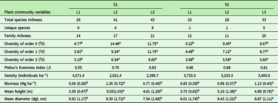
In S1 we recorded 1384 individuals representing 53 species (of which eight remained as unidentified morphospecies) and 24 families, with 29 species occurring in L1, 41 in L2 and 43 in L3 (Table 1, Appendix 1). In S2 we recorded 1730 individuals representing 38 species (including five that remained unidentified) and 16 families, with 25 species occurring in L1, 28 in L2, and 33 in L3 (Table 1, Appendix 1). The values of 0D, 1D and 2D true diversities differed significantly between altitudes (Table 1); moreover, biomass, mean height and mean diameter also differed between altitudinal levels, with the highest mean values found in L2 and L3 (Table 1). Species with the highest densities on the two mountains were Croton blanchetianus, Cenostigma pyramidale and Allophylus sp. in S1, and Croton heliotropiifolius, Tacinga palmadora and Aspidosperma pyrifolium in S2.
Diversity and structural variables of the woody (tree + shrub) community, including all live individuals ≥ 1 m in height and with stem diameter at ground level (dgl) ≥ 3 cm, in the Serra de Bodocongó (S1) and Serra da Arara (S2) mountains, Paraíba State, Brazil. For the three bottom variables, values are means (SD in parentheses). L1, low altitudinal belt; L2, middle altitudinal belt; L3, high altitudinal belt. For each variable, superscript letters indicate significantly different means between altitudinal belts, according to Kruskal–Wallis or Tukey tests

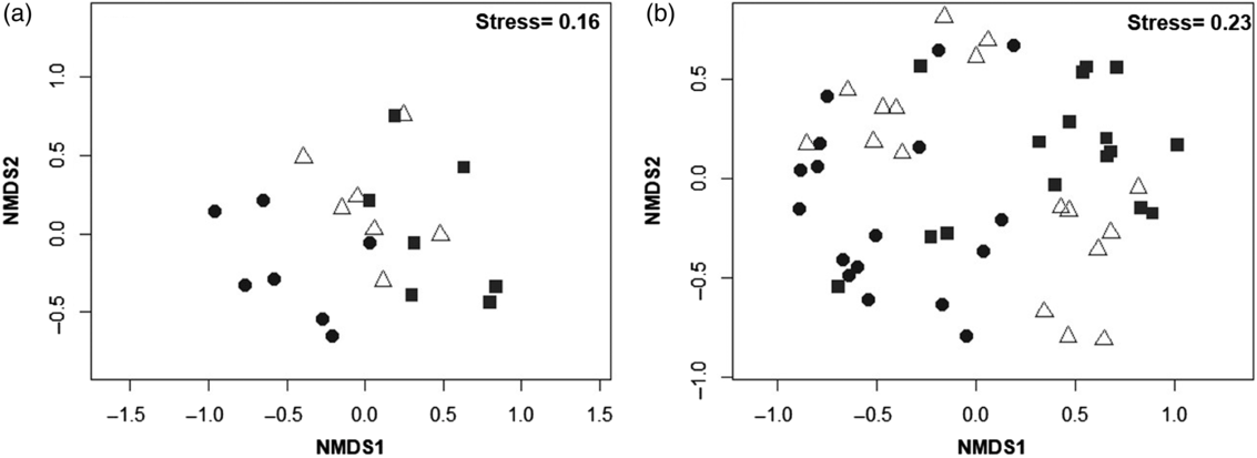
The NMDS showed a clear separation of altitudinal levels, with the formation of three floristic groups for each of the two mountains (Figure 2a, b). Ordination stress was 0.16 for S1 and 0.23 for S2, indicating acceptable sample segregation along the altitudinal gradients. The three altitudinal levels were significantly different in terms of their composition and abundance (S1, Pseudo-F2,18 = 7.76, P = 0.001; S2, Pseudo-F2,18 = 33.87, P = 0.0002).
Floristic groups corresponding to three altitudinal levels in Serra de Bodocongó (a) and Serra de Arara (b) mountains, in the semi-arid region of NE Brazil. The samples (plots) are ordered for each of the two dimensions produced by a non-metric multi-dimensional scaling (NMDS) ordination performed using an abundance-based Bray–Curtis similarity matrix and altitude (see Methods for details). Circles, L1 plots; triangles, L2 plots; squares, L3 plots.

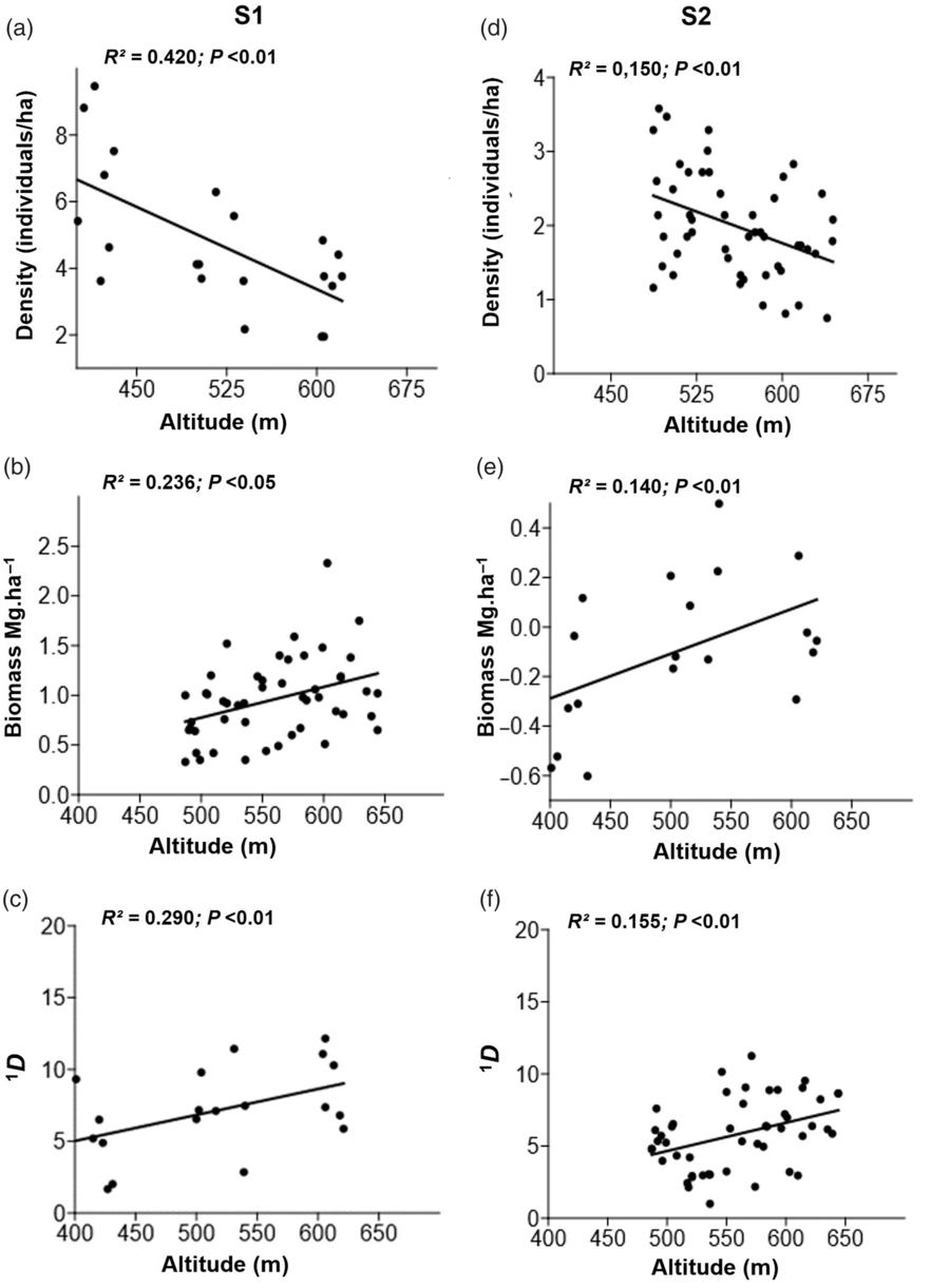
True diversity for all three diversity orders, biomass, mean height and mean dgl differed significantly along the altitudinal gradient in both mountains (Table 1). At the highest altitudinal levels (L2 and L3), we recorded larger values for dgl and tree height for S1 (Table 1), as well as higher species diversity and biomass (Figure 3b, c, e, f). The areas located at the lower altitudes (L1) had higher densities and more multi-stemmed individuals, and were dominated by Croton blanchetianus and C. pyramidale in S1, and C. heliotropiifolius in S2. On both mountains these species had individuals at all altitudinal levels, notwithstanding their highest densities at the lowest altitudes. The low R2 values obtained at S2 (<0.20) for density and species diversity indicate the low predictive power of altitude.
Linear regressions of community structural (a, b, d, e) and diversity (c, f) variables on altitude for the woody community in two mountains of Brazil’s semi-arid region. (a, b, c) Bodocongó site; (d, e, f) Arara site. 1D, exponential Shannon entropy.

Edaphic variables
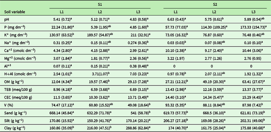
At S1 we recorded the highest values for K and H+Al, with pH ranging from 4.83–5.41 (Table 2). At S2 we recorded high pH, P, Ca, OM and V values, with significant differences among altitudinal levels for pH, Na, OM, sand and silt (Table 2). In turn, for S1, significant differences among altitudinal levels were found for P, K, Na, H+Al, OM, V, sand and clay (Table 2). Mean V values for S2 were high, indicating higher cationic nutrient fertility than at S1. However, fertility showed little variation among altitudinal belts in S2 compared with S1 (Table 2).
Chemical variables and soil texture of composite topsoil samples (0–20 cm) in Serra de Bodocongó (S1) and Serra da Arara (S2) mountains, Paraíba, Brazil. Values are means (SD in parentheses). H+Al, potential acidity; Al, exchangeable acidity; TEB, total exchangeable bases; CEC, cation exchange capacity; V, base saturation; OM, organic matter. L1, low altitudinal belt; L2, middle altitudinal belt; L3, high altitudinal belt. For each variable, superscript letters indicate significantly different means between altitudinal belts, according to Kruskal–Wallis or Tukey tests

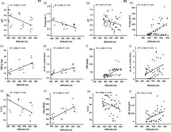
Linear regressions showed that pH, P, OM and base saturation varied significantly with altitude, with soil fertility being lowest at the highest altitudes (Figure 4a, b, e, g, h, k). Regarding soil texture, this soil property varied significantly along the altitudinal gradient at S1 (sand, F = 8.427, P < 0.001; clay, F = 11.64, P < 0.001). In the case of S2, even though regressions of clay and sand fractions on altitude were not significant (P > 0.05), we found significant differences among altitudinal belts for sand (F = 7.08, P < 0.001). Also, we confirmed the existence of steeper slopes as altitude increased in both areas (S1, R2 = 0.327; P < 0.05; S2, R2 = 0.575; P < 0.05).
Linear regressions between altitude and edaphic variables of the woody community along two altitudinal gradients in Brazil’s semi-arid region. (a–f) Bodocongó mountain; (g–l) Arara mountain. H+Al, potential acidity; V, base saturation; OM, organic matter.

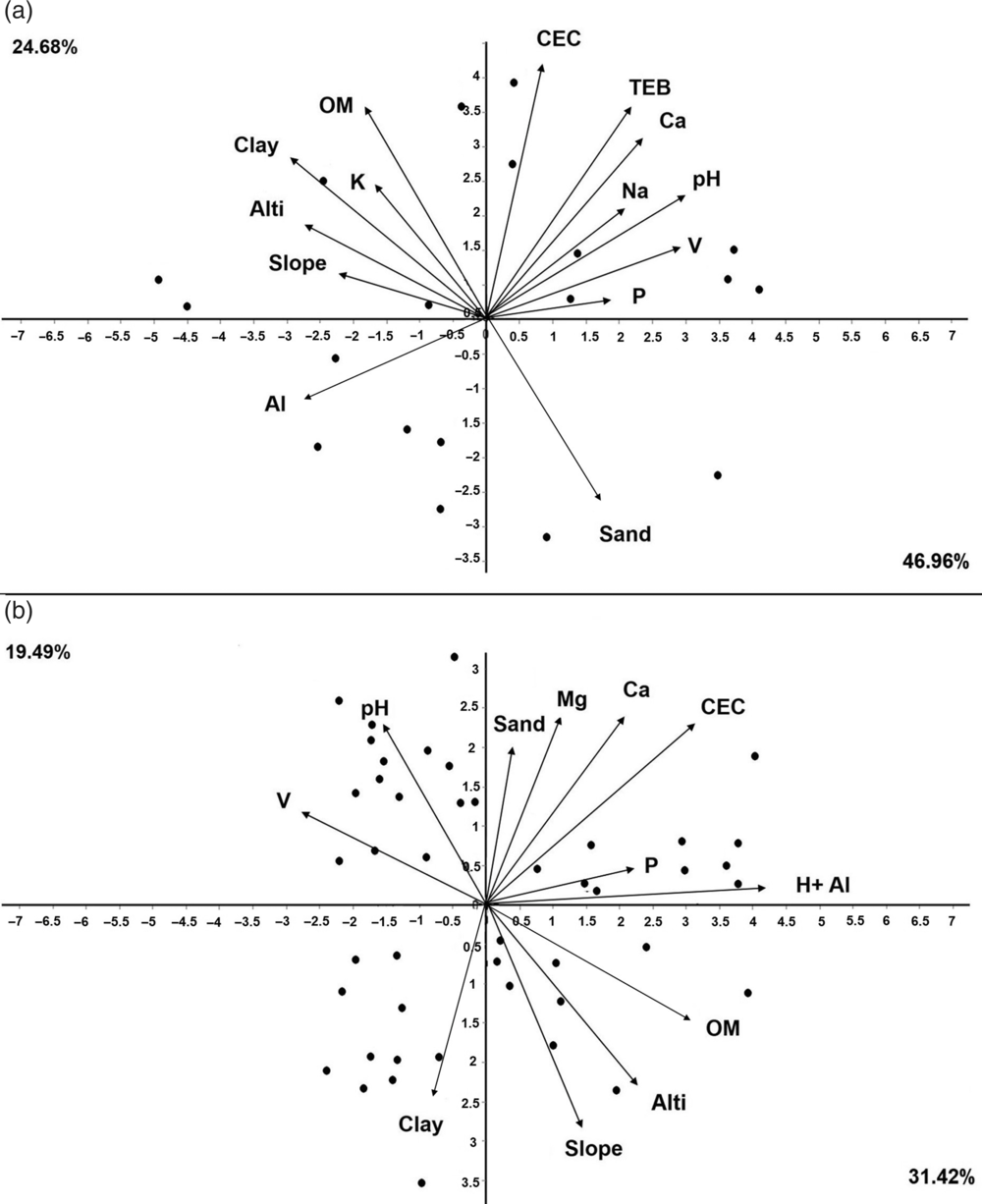
PCA resulted in the segregation of two main gradients regarding soil conditions in the study region. For S1, the first two PCs explained 71.64% of total variation: PC1 (46.96%) was positively related with sand, P, V, Na, pH, Ca, TEB and CEC, while PC2 (24.68%) was positively related with OM, clay, Al, K, slope and altitude (Figure 5a). For S2, PCA explained 50.91% of variation in soil properties; a considerable fraction of all variance was explained by PC1 (31.42%), which was positively correlated with Na, P, OM, Ca, Mg, CEC and H+Al, sand, slope and associated with areas located at higher altitudes, whereas PC2 (19.49%) was associated with base saturation (V), clay and pH, both of which were negatively related to altitude (Figure 5b).
Principal component analyses (PCA) of topsoil edaphic variables (0–20 cm) to examine their correlations for (a) Bodocongó (S1), and (b) Arara (S2) sites. H+Al, potential acidity; Al, exchangeable acidity; TEB, total exchangeable bases; CEC, cation exchange capacity; V, base saturation; OM, organic matter; Alti, altitude.

Vegetation–soil relations
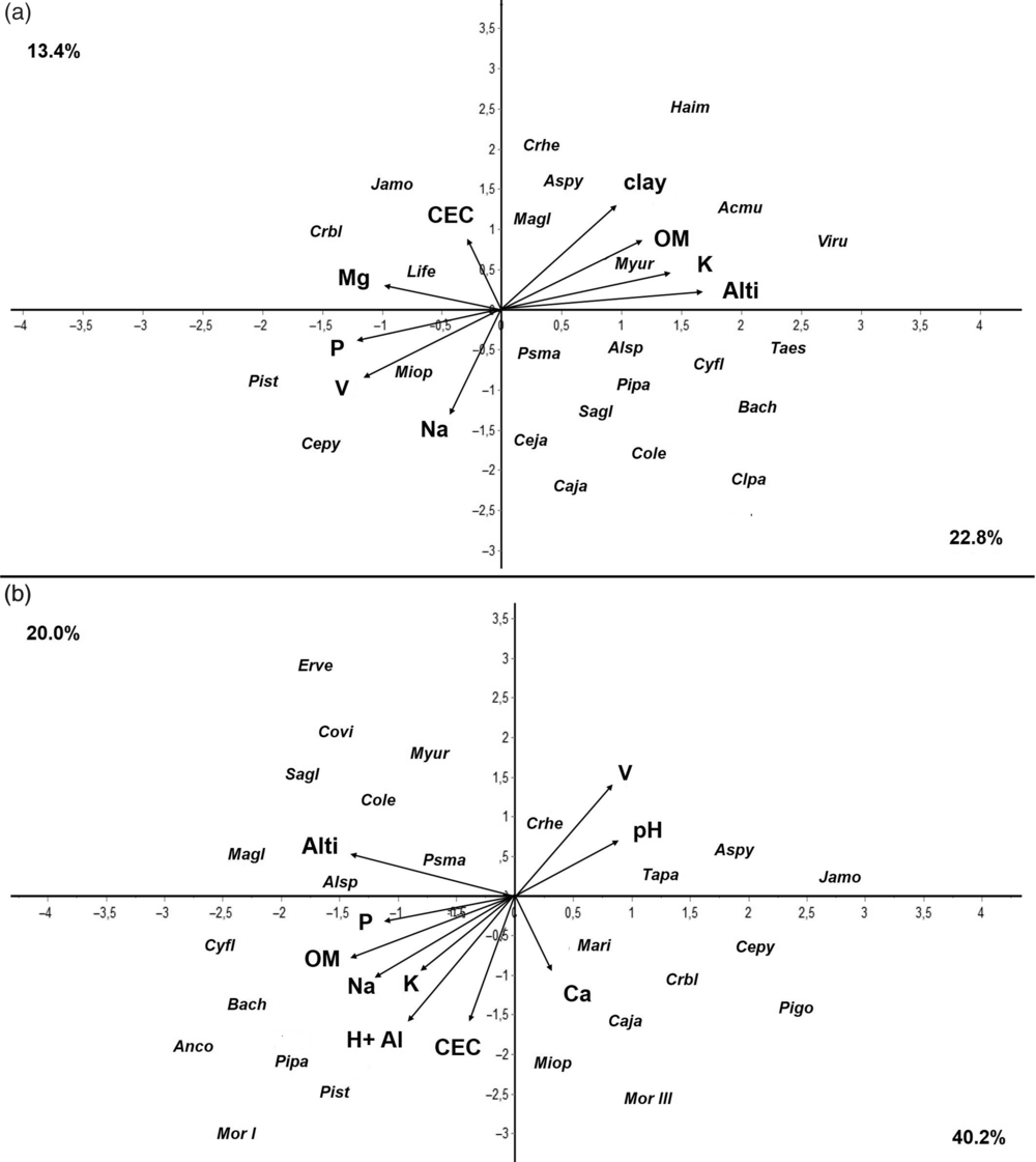
The CCA ordination clearly separated two groups of species according to the edaphic and altitudinal variation present in the two mountains (Figure 6). For S1, the two first axes jointly explained 36.2% of total variance in soil properties and species across altitudinal belts. Axis 1 (22.8%) was positively associated with Mg, Na, Ca, P, V, sand and silt, and negatively so with H+Al, OM and clay; in turn, Axis 2 (13.4%) was significantly associated with CEC only (Figure 6a). Species of the studied plant communities segregated in two distinct floristic groups. The first one included Bauhinia cheilantha, Capparis jacobinae, Clusia paralicola, Commiphora leptophloeos, Pseudobombax marginatum, Cynophalla flexuosa, Croton heliotropiifolius, Manihot glaziovii, Handroanthus impetiginosus, Aspidosperma pyrifolium, Allophylus sp., Myracrodruon urundeuva, Vitex rufescens, Sapium glanduloson, Cereus jamacaru, Talisia esculenta, Pilosocereus pachycladus and Acalypha multicalis, all of them associated with higher H+Al, OM and clay contents. The second group comprised Jatropha mollissima, Piptadenia stipulacea, Croton blanchetianus, Cenostigma pyramidale and Mimosa ophthalmocentra, which are dominant in low-altitude communities and correlated with higher Mg, Na, Ca, P, V, CEC, sand and silt contents.
Canonical correspondence analyses (CCA) based on the numbers of individuals of plant species and edaphic variables of the surface-layer (0–20 cm) in S1 (a) and S2 (b). Soil variables are indicated by arrows: H+Al, potential acidity. Al, exchangeable acidity; CEC, cation exchange capacity; V, base saturation; OM, organic matter; Alti, altitude. Species labels are abbreviated by taking the first two letters from the generic and specific epithets, respectively, of species names (full names are given in Appendix 1). Species with fewer than 10 recorded individuals were excluded from the analysis to avoid spurious effects caused by rare species.

For S2, the two first axes jointly explained 60.2% of the total variance (Figure 6b). Species placed on the right part of axis 1 (40.2%) are abundant in low-altitude sites (e.g. Aspidosperma pyrifolium, Croton blanchetianus, Mimosa ophthalmocentra, Tacinga palmadora, Morphospecies III, Capparis jacobinae, Croton heliotropiifolius, Pilosocereus gounellei and Cenostigma pyramidale), and were positively associated with Ca, Mg, V and pH. Those concentrated on the left part of the ordination space, including Anadenanthera colubrina, Piptadenia stipulacea, Pseudobombax marginatum, Pilosocereus pachycladus, Morphospecies I, Cochlospermum vitifolium, Cynophalla flexuosa, Manihot glaziovii, Commiphora leptophloeos, Myracrodruon urundeuva, Erythrina velutina and Bauhinia cheilantha, are positively related with Na, OM, C, H+Al, CEC and altitude. Axis 2 explained 20.0% of total variance.
Discussion
The floristic and structural information gathered in this study sheds new light on the role of edaphic variables in the structuring of plant communities through the analysis of the soil-altitude-vegetation tripartite relationship. Our results revealed the magnitude of the changes under the different edaphic conditions measured along two altitudinal gradients and suggest the potential of soil to promote plant community heterogeneity in mountainous areas of Brazil’s semi-arid Caatinga.
The segregation of distinct floristic groups by NMDS sample ordination confirms the influence of altitude on species distribution, reflecting differences among the pre-established levels. Altitude has been recognized as an environmental gradient associated with floristic and physiognomic changes in tropical forests (Salas-Morales & Meave Reference Salas-Morales and Meave2012, Sanchez et al. Reference Sanchez, Pedroni, Eisenlohr and Oliveira-Filho2013, Vázquez & Givnish Reference Vázquez and Givnish1998), even at small scales (Gallardo-Cruz et al. Reference Gallardo-Cruz, Pérez-García and Meave2009), and our results are in agreement. Previous studies conducted on the mountains of the Caatinga region have shown higher species richness compared with areas located on flat terrain (Araújo et al. Reference Araújo, Parente, Éder-Silva, Ramalho, Dantas, de Andrade and da Silva2012, Calixto Júnior & Drumond Reference Calixto Júnior and Drumond2011, Guedes et al. Reference Guedes, Zanella, Costa Júnior, Santana and Silva2012, Lopes et al. Reference Lopes, Ramos and Almeida2017, Silva et al. Reference Silva, Lopes, Lopez, Melo and Trovão2014). Also, they have repeatedly reported an increase in species richness with altitude, in disagreement with most observed patterns globally (Lomolino Reference Lomolino2001, Manish et al. Reference Manish, Pandit, Telwala, Nautiyal, Koh and Tiwari2017). Besides such increase in species richness towards higher altitudes, our results showed decreasing soil fertility in the same direction. These results are consistent with other studies conducted along altitudinal gradients in Brazil and elsewhere (Kichenin et al. Reference Kichenin, Wardle, Peltzer, Morse and Freschet2013, Maragon et al. Reference Maragon, Soares, Feliciano, Lani and Matos2013, Rodrigues et al. Reference Rodrigues, Carvalho, Oliveira-Filho and Curi2007, Wilcke et al. Reference Wilcke, Yasin, Schmitt, Valarezo, Zech, Beck, Bendix, Kottke, Makeschin and Mosandl2008), which report lower plant diversity in areas of high fertility.
Although the higher base saturation observed downslope might indicate catenary nutrient translocation (Martins et al. Reference Martins, Silva, de Souza and Neto2003, Souza et al. Reference Souza, Lelis, Schaefer, Souza and Meira-Neto2012), this pattern could also be due to higher precipitation and soil leaching at higher altitudes, or to the presence of more dystrophic parent material in those places. Being located in an area of relatively high precipitation within the Caatinga (600 mm), S1 may be more strongly affected by soil leaching, which could explain the inverse relationship between P and altitude observed there, in contrast to the finding for S2, where P increased with increasing altitude and organic matter content. Considering the trend of species richness to be higher towards the tops of both mountains, it seems that despite the key role of P for vegetation development (Malhotra et al. Reference Malhotra, Sharma, Pandey, Hasanuzzaman, Fujita, Oku, Nahar and Hawrylak-Nowak2018, Pellegrini Reference Pellegrini2016), this element is not the main driver of species richness patterns in these environments. Low pH values in L3 are associated with high Al availability, which may ultimately affect the growth and distribution of some species (Viani et al. Reference Viani, Rodrigues, Dawson, Lambers and Oliveira2014). In any case, further edaphological research is needed in these mountains to clarify this issue.
Edaphic factors (particularly soil fertility) provided sufficient evidence to explain the floristic and structural differences between the two mountains studied. For example, soils at S2 were more fertile compared with S1, likely favouring the dominance of some species (e.g. Croton blanchetianus and C. heliotropiifolius), while inhibiting others (e.g. Cochlospermum vitifolium, Commiphora leptophloeos, Myracrodruon urundeuva, Pseudobombax marginatum and Schinopsis brasiliensis). Moreover, the narrower altitudinal range in S2 results in a relatively more homogeneous environment, which reduces the possibility of altitudinal niche specialisation (Lopes Reference Lopes2017, Rodrigues et al. Reference Rodrigues, Schaefer, Silva, Ferreira-Júnior, Santos and Neri2018, Tilman Reference Tilman2004), ultimately likely resulting in S2 hosting fewer species than S1. Yet, the linear regressions of structural variables on altitude at both sites suggest that the variation in vegetation structure is similar along the two gradients, even considering the limited altitudinal range that they encompass.
Heterogeneity in nutrient availability is not only reflected in differences in species richness at different altitudes, which results from fine specialization of many species to particular edaphic conditions (Bohlman et al. Reference Bohlman, Laurance, Laurance, Nascimento, Fearnside and Andrade2008, Born et al. Reference Born, Pluess, Burslem, Nilus, Maycock and Ghazoul2014, van der Putten et al. Reference Van der Putten, Bardgett, Bever, Bezemer, Casper, Fukami, Kardol, Klironomos, Kulmatiski, Schweitzer, Suding, Van De Voorde and Wardle2013). Species densities also changed with altitude in both mountains, which may be related to resource limitations or to the presence of stronger competitors that inhibit the expansion of individuals to some altitudinal belts (Boulangeat et al. Reference Boulangeat, Lavergne, Garraud and Thuiller2012, Olsen & Klanderud Reference Olsen and Klanderud2014). Also, in addition to variation in soil factors, the highest portions of the altitudinal gradients in the Brazilian semi-arid region are favoured by a considerable reduction in water stress (Lopes et al. Reference Lopes, Ramos and Almeida2017, Sampaio Reference Sampaio, Gariglio, Sampaio, Cestaro and Kageyama2010).
The lower diversity observed at lower altitudes (L1), where soils are more fertile, may be due to stronger dominance of some species exposed to high resource supply. Under such conditions all species have similar colonization opportunities, yet few succeed in attaining dominance rapidly, particularly in the presence of human disturbance (Huston Reference Huston1979, Reference Huston2014). This seems to be the case of Croton blanchetianus, C. heliotropiifolius and Cenostigma pyramidale, all of which are generalist species and behave as pioneers in anthropic areas of the Caatinga (Araújo et al. Reference Araújo, Parente, Éder-Silva, Ramalho, Dantas, de Andrade and da Silva2012, Ribeiro et al. Reference Ribeiro, Arroyo-Rodríguez, Santos, Tabarelli and Leal2015, Rito et al. Reference Rito, Tabarelli and Leal2017b). Although these three species occurred over the entire altitudinal gradient at both sites, their densities and basal areas peaked at the lowest altitudes. The largest anthropic impacts occur in L1 (Lopes et al. Reference Lopes, Ramos and Almeida2017) and at both sites species of the genus Croton were dominant, confirming the dominance of the Euphorbiaceae family in disturbed areas of the Caatinga (Rito et al. Reference Rito, Tabarelli and Leal2017b). When successful colonizers become dominant, they constrain the development of species less tolerant to the environment (Büchi & Vuilleumier Reference Büchi and Vuilleumier2014), often through monopolization of essential resources (Huston Reference Huston1979). Besides the influence of human disturbance on the distribution patterns of these three species, as discussed earlier, our results also suggest that they are better competitors on fertile soils, which guarantees their stronger dominance and confers on them higher competitive advantages in this benign habitat.
Soil granulometry is also a key factor in the emergence of species richness and composition patterns in the plant community (Bueno et al. Reference Bueno, Neves, Souza, Oliveira Junior, Damasceno Junior, Pontara, Laura and Ratter2013, Decker & Boerner Reference Decker and Boerner2003). Soil texture directly influences porosity and consequently the availability of water, the status of P, N, Al and organic matter, as well as the activity of edaphic microorganisms (Galantini & Suñer Reference Galantini and Suñer2008, Galantini et al. Reference Galantini, Senesi, Brunetti and Rosell2004). The highest Al, H+Al, OM and clay contents were found in L3, and these soil factors showed significant and positive regressions with altitude (except for clay in S2, which was not significantly correlated with it). Clay particles ensure a better soil structure, through the formation of micro- and macro-aggregates that result in good porosity and consequently can be reflected in higher species richness in these environments (Galantini et al. Reference Galantini, Senesi, Brunetti and Rosell2004).
Higher OM contents may be associated with larger clay fractions in the soil, which could hamper water infiltration and affect OM decomposition, ultimately leading to its accumulation. Larger OM values, along with low pH (Figure 4a, g, c, i), intensify soil acidity and increase Al and H+Al availability (Rodrigues et al. Reference Rodrigues, Schaefer, Silva, Ferreira-Júnior, Santos and Neri2018). Many tropical soils are typically acidic (Sanchez & Logan Reference Sanchez, Logan, Lal and Sanchez1992), with Ca and Mg being negatively related with each other due to competition for adsorption sites in the soil and absorption by plant roots (Zhu et al. Reference Zhu, Riley, Tang and Koven2016). These nutrients are important in structuring vegetation and soils, besides affecting soil pH and consequently pH-controlled processes (Schaefer et al. Reference Schaefer, Amaral, Mendonça, Oliveira, Lani, Costa and Fernandes-Filho2008).
Besides nutrient availability, the occurrence of anthropic disturbances at the lowest altitudes (Méndez-Toribio et al. Reference Méndez-Toribio, Meave, Zermeño-Hernández and Ibarra-Manríquez2016, Silva et al. Reference Silva, Lopes, Lopez, Melo and Trovão2014) may be at least partly responsible for the increasing dominance of some species in these areas (e.g. Croton blanchetianus, C. heliotropiifolius, Allophylus sp. and Cenostigma pyramidale), while curbing the abundances of disturbance-intolerant species, such as Bauhinia cheilantha, Myracrodruon urundeuva, Pseudobombax marginatum and Schinopsis brasiliensis. Interestingly, the latter four species are common in well-preserved Caatinga vegetation (Ribeiro et al. Reference Ribeiro, Arroyo-Rodríguez, Santos, Tabarelli and Leal2015), and their abundances peak at the highest altitudes (Lopes et al. Reference Lopes, Ramos and Almeida2017). Generalist species have broad tolerances to different environments and possess life history traits that allow them to increase reproductive success under certain disturbance regimes (Devictor et al. Reference Devictor, Julliard and Jiguet2008, Rito et al. Reference Rito, Tabarelli and Leal2017b, Verberk et al. Reference Verberk, Van Der Velde and Esselink2010); also, these species become abundant or even dominant rapidly, ultimately reducing species richness locally (Büchi & Vuilleumier Reference Büchi and Vuilleumier2014, Tabarelli et al. Reference Tabarelli, Lopes and Peres2008).
Unexpectedly, the highest plant diversity was recorded on the less fertile and more acidic soils at higher altitudes in both mountains. This is likely related to niche partitioning (Lopes Reference Lopes2017, Ricklefs Reference Ricklefs2015), frequently observed in heterogeneous environments (Boulangeat et al. Reference Boulangeat, Lavergne, Garraud and Thuiller2012, Tilman Reference Tilman2004). In fact, the CCA revealed the effects of edaphic variables on the configuration of floristic arrays. At S1, for example, Simaba cuneata and Handroanthus impetiginosus occurred exclusively in high-altitude plots of L3, where H+Al, OM and clay contents were highest, suggesting strong edaphic specialization (van der Putten et al. Reference Van der Putten, Bardgett, Bever, Bezemer, Casper, Fukami, Kardol, Klironomos, Kulmatiski, Schweitzer, Suding, Van De Voorde and Wardle2013). The high-altitude plant diversity peak illustrates the complexity of mountains in the Caatinga as ecological systems. This finding confirms a species richness pattern little known in the literature (Rahbek Reference Rahbek1995), which appears to be caused by the edaphic variation along the topographic gradient.
Conclusions
In synthesis, our results strongly suggest that the mountains of Brazil’s semi-arid region may act as refugia for Caatinga’s plant biodiversity in the face of human disturbance, and represent ideal environments for investigating the effects of global climate change on biodiversity. From a geological viewpoint, these environments will offer valuable information to support future efforts to trace the evolutionary history of Caatinga, including both soil and vegetation, through the analysis of pedological and geological processes associated with the formation of the Brazilian semi-arid region.
In this study we demonstrate the role of edaphic variables on patterns of plant species richness and diversity, and on structural attributes of the communities that occur along the altitudinal gradient. However, future studies should examine subsoil data as well, since a vertical analysis encompassing the full soil depth may provide relevant information on soil water retention capacity and available water, as well as an assessment of the subsoil contribution to nutrient supply for vegetation. Moreover, it will be necessary to evaluate the role of other environmental variables, such as microclimatic factors, and the effects of anthropic disturbance, in order to better understand multiple species’ responses to these variations through their functional traits. Lastly, all these efforts should attempt to unravel the synergistic effects of all environmental variables affecting the assembly of plant communities in the Brazilian semi-arid region.
Acknowledgements
We are grateful to Vitor Leite Martins for logistical support that enabled access to the study areas. Camila Santos Albuquerque, Sonally Silva da Cunha, D’Ávilla Ruama Fernandes Lopes Gomes, Pablo José da Silva, Brenda Kyara and Iran da Costa Leite Neto assisted with fieldwork. Professor João José Lelis Leal de Souza provided valuable considerations on geomorphology. Special thanks go to the reviewers of this paper for their valuable suggestions and criticism. We are grateful to Laboratório de Química e Fertilidade do Solo of Universidade Federal da Paraíba for their help with soil analyses.
Financial support
CNPq provided financial support for this study (Grant No. 07629-2014) and awarded a productivity grant to SFL.
Appendix 1 Checklist of species recorded along two altitudinal gradients along with their total abundances in each of them, for the Bodocongó (S1) and Arara (S2) mountain sites, Paraíba state, NE Brazil