

1 Introduction
Jet control is a long-standing research problem, generally motivated by two main purposes: increasing jet mixing or reducing jet noise. These two objectives are usually opposed.
One effective way of enhancing jet mixing is to increase the global jet spreading, and thus the size of its mixing layer region. To do so, one relies on the leading large global structures of the jet, the vortex rings (Hussain & Zaman Reference Hussain and Zaman1980; Zaman & Hussain Reference Zaman and Hussain1980). Imposing an axial forcing at the jet inlet controls the frequency at which the vortex rings are generated, and therefore their spacing. Additional actuation of the vortex ring dynamics then allows the jet spreading and mixing to be further controlled. Several attempts that have been carried out in the literature are now detailed.
A first possibility is to rely on the pairing instability of vortices. At some parameter settings, an axisymmetric time-periodic array of vortices is globally unstable in a Floquet sense (Floquet Reference Floquet1883; Shaabani-Ardali, Sipp & Lesshafft Reference Shaabani-Ardali, Sipp and Lesshafft2019): ring vortices, while being advected downstream, merge two by two, leading to thicker ring vortices and to a larger mixing region. In stable cases, it is still possible to trigger pairing by adding an axisymmetric subharmonic forcing at the inlet (Hussain & Zaman Reference Hussain and Zaman1980; Zaman & Hussain Reference Zaman and Hussain1980). Depending on the phase shift between the fundamental and the subharmonic forcing, such forcing will either promote or inhibit pairing, as shown by Arbey & Ffowcs Williams (Reference Arbey and Ffowcs Williams1984) or Raman & Rice (Reference Raman and Rice1991).
Another, more effective possibility is to generate bifurcating and blooming jets. These jets, first studied by Lee & Reynolds (Reference Lee and Reynolds1985), are the result of jet forcing that combines axisymmetric and helical components, at frequencies  $f_{a}$ and
 $f_{h}$. The difference between these two kinds of flow response lies in the ratio of frequencies
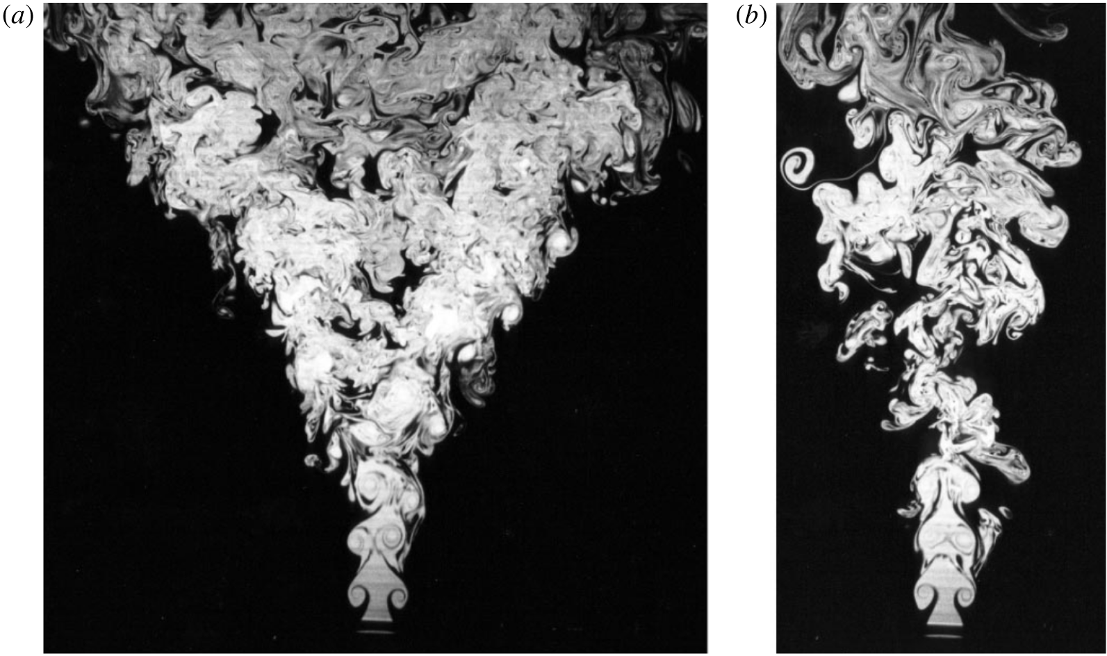
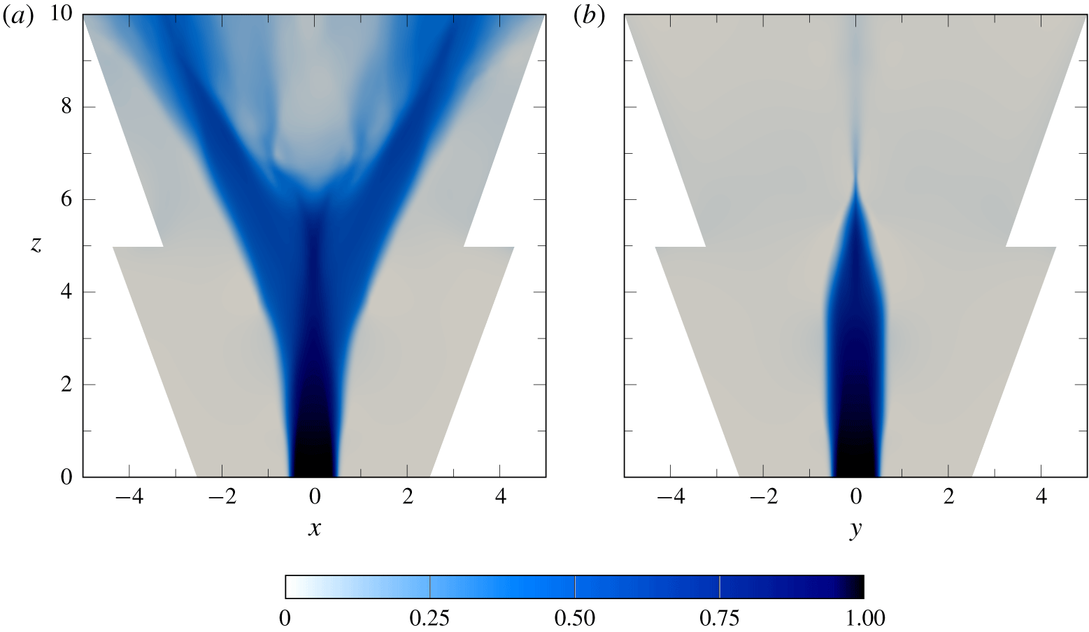
 $R_{f}=f_{a}/f_{h}$. In the case of jet bifurcation, this ratio is fixed at two: each vortex generated is alternatively shed to the right and to the left, and then, by mutual induction, they further depart from the jet axis, leading to the scenario shown in figure 1. This jet strongly flares in the shedding plane, called hereafter the bifurcating plane, whereas it does not display any additional flaring in the normal plane, called the bisecting plane. This bifurcation scenario, introduced by Lee & Reynolds (Reference Lee and Reynolds1985) has been analysed physically by Parekh, Reynolds & Mungal (Reference Parekh, Reynolds and Mungal1987), Parekh, Leonard & Reynolds (Reference Parekh, Leonard and Reynolds1988). They stated that ‘the shear layer rolls up into a periodic array of vortex rings in response to the axial forcing. The helical or transverse forcing displaces these rings eccentrically. The resulting staggered array of rings is unstable. As a result, the rings tilt away from each other until initially adjacent rings eventually propagate along two different trajectories’, as shown in figure 2. Parekh et al. (Reference Parekh, Leonard and Reynolds1988) have shown that the bifurcating jet mechanism can also be triggered at large Reynolds number, and is not restricted to small Reynolds values. By fixing
 $R_{f}$ to three, trifurcating jets have been observed (Lee & Reynolds Reference Lee and Reynolds1985), but they do not display as much flaring as bifurcating jets.
Bifurcating (a) and bisecting (b) plane views of a bifurcating jet at  $Re=4300$ with
 $R_{f}=2$. From Lee & Reynolds (Reference Lee and Reynolds1985).

Schematic of a bifurcating jet, from Lee & Reynolds (Reference Lee and Reynolds1985).

This phenomenon, quite promising for mixing enhancement, has been deeply analysed in a series of papers. A comprehensive review can be found in Reynolds et al. (Reference Reynolds, Parekh, Juvet and Lee2003). Some authors have tried to extend this method to compressible settings (Tyliszczak & Boguslawski Reference Tyliszczak and Boguslawski2006, Reference Tyliszczak and Boguslawski2007) or to other methods of forcing, such as flapping motions (Danaila & Boersma Reference Danaila and Boersma1998, Reference Danaila and Boersma2000; da Silva & Métais Reference da Silva and Métais2002; Gohil, Saha & Muralidhar Reference Gohil, Saha and Muralidhar2010; Gohil & Saha Reference Gohil and Saha2019). From all these studies, it can be concluded that a convenient band of axisymmetric forcing Strouhal numbers to observe bifurcating jets is  $0.4\lesssim St\lesssim 0.6$, with peak spreading occurring around
 $St_{a}=0.5$. The existence of this band has been early understood by Lee & Reynolds (Reference Lee and Reynolds1985): ‘When the vortex rings are spaced far apart, the interaction between them is small. When the spacing is smaller, the interaction is stronger. When the rings are spaced closer and closer, a critical value is reached where the rings turn and run into each other without ever escaping’.
Nevertheless, other ways of achieving bifurcating jets have been developed in the 1990s. Pfizenmaier, Simon & Monkewitz (Reference Pfizenmaier, Simon and Monkewitz1993) relied, with a single frequency forcing, on the spiral instability mode of a jet diffusion flame to achieve a flapping motion. Another method employs radial forcing. Experimentally, this is achieved by placing fluidic actuators along a ring around the jet inlet. These actuators pulse flow at a given frequency and are in phase opposition. Parekh et al. (Reference Parekh, Kibens, Glezer, Wiltse and Smith1996) have shown experimentally in a compressible setting (Mach number  $Ma=1.47$) that with a minimal mass flux, of about 1 % of the mean flow flux, such forcing dramatically changed the dynamics of the jet and its mixing properties. In similar settings, Freund & Moin (Reference Freund and Moin1998, Reference Freund and Moin2000) have shown numerically that such actuation was able to drastically reduce the size of the potential core and to enhance mixing for all the metrics they considered, such as mean mass flux or scalar dissipation. Their instantaneous flow contours resemble traditional bifurcating jet flows, with vortices shed in a preferential plane entraining vortices. Simulations have also been carried out for such forcing behind real jet engines (Smith, Cain & Chenault Reference Smith, Cain and Chenault2001). In these studies, the most receptive Strouhal numbers
 $St_{h}$ are of the order of 0.2–0.25. This frequency is similar to the helical forcing frequencies of the bifurcating jets with axial forcing (
 $St_{h}$ of the order of 0.2–0.3), reinforcing the idea that similar mechanisms play a role in these two flows. Still another method relies on both passive and active control techniques, by combining axisymmetric forcing (that triggers vortex rings) with nozzle modifications to induce non-axisymmetric perturbations on the rings. Several shapes have been tested, such as chevrons (vortex generators) in the nozzle (Zaman, Reeder & Samimy Reference Zaman, Reeder and Samimy1994; Zaman & Raman Reference Zaman and Raman1997), stepped and sawtooth nozzles (Longmire & Duong Reference Longmire and Duong1996), or inclined nozzles (Webster & Longmire Reference Webster and Longmire1997).
For both of these methods, bifurcating two-frequency forcing and radial forcing, some studies have attempted to optimise the spreading in bifurcating and blooming jets. Koumoutsakos, Freund & Parekh (Reference Koumoutsakos, Freund and Parekh1998) have tried to apply evolution strategies to optimise the bifurcating jet generated by a radial forcing. They also used vortex filament algorithms to optimise blooming jets. However, instead of carrying out global optimisation, they optimised the parameters (amplitude, frequency, phase) of a given forcing shape. Similarly, Hilgers & Boersma (Reference Hilgers and Boersma2001) have applied genetic algorithms to flapping and bifurcating perturbations. In all of these studies, the computational cost was prohibitive, owing to the cost of three-dimensional resolved direct numerical simulations (DNS) and the large numbers of runs needed for an optimisation. Several objective functions have been introduced: the volume integral of radial velocity, the passive scalar concentration in the outer domain or the radial displacement of vortices, and difficult compromises had to be made to mitigate the computational burden of such computations. In a later study, Tyliszczak & Geurts (Reference Tyliszczak and Geurts2014) carried out a parametric analysis of the bifurcating jet, at  $Re=4300$ and 10 000. They studied the influence of the amplitude, the forcing frequency and the phase of the forcing and of the turbulence level. Their main conclusions are, for the bifurcating jet, that the forcing amplitude must be larger than the inlet turbulence level, and that a larger forcing amplitude leads to bifurcation over a wider range of Strouhal numbers. Experimentally, Wu et al. (Reference Wu, Fan, Zhou, Li and Noack2018) carried out an optimisation of mixing in a turbulent jet, based on machine learning control (MLC). This flow was actuated by a single minijet inside the nozzle, oriented in the radial direction. Through the automated MLC procedure, it was found that the optimal forcing frequency, which led to maximal mixing, corresponded to exactly half the frequency that dominated the unforced jet, associated with axisymmetric vortex formation. The optimal radial actuation of this turbulent jet triggered a clear bifurcation (see figure 10 of Wu et al. Reference Wu, Fan, Zhou, Li and Noack2018).
In the case of two-frequency forcing strategies, blooming jets occur when  $R_{f}=f_{a}/f_{h}$ is no longer integer: as
 $f_{a}$ and
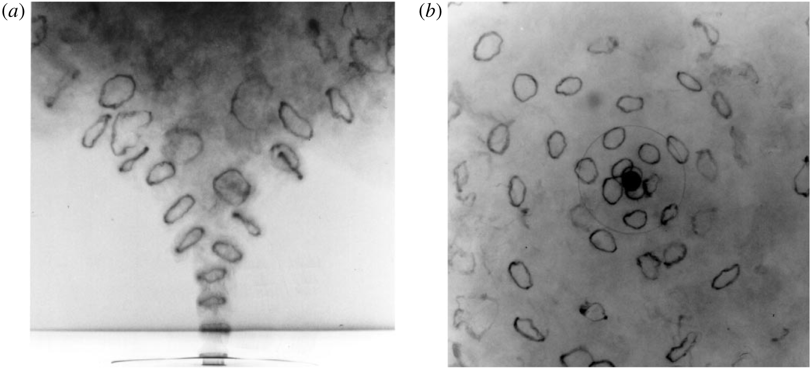
 $f_{h}$ are no longer commensurate, there is no preferential plane for bifurcation, and the vortices are evolving in the full three-dimensional space. Therefore, the jet envelope becomes conical, ensuring maximum mixing of the jet, as shown in figure 3. Lee & Reynolds (Reference Lee and Reynolds1985) have found that blooming, in their experimental setting, occurs for
 $1.6<R_{f}<3.2$ and
 $0.35<St_{a}<0.75$. This scenario has gained attention recently with the articles of Tyliszczak (Reference Tyliszczak2015) and Gohil, Saha & Muralidhar (Reference Gohil, Saha and Muralidhar2015). Both explain that, although at first glance the rings seem to cover uniformly all azimuthal directions, they form a distinct number of branches that can be directly linked to
 $R_{f}$. Recently, the forcing of organised multi-armed jets with up to 13 branches has been investigated by Tyliszczak (Reference Tyliszczak2018). The frequency ratio also determines the spreading angle between two consecutive vortices; if these vortices are on two sufficiently separated branches, these branches will not interact with one another, leading to a clear blooming.
Side (a) and top (b) view of a blooming jet at  $Re=4300$ with
 $R_{f}=2.4$. From Lee & Reynolds (Reference Lee and Reynolds1985).

In the present study, our purpose is to find the optimal helical inlet forcing for triggering jet bifurcation. To do so, we will rely on the bifurcation mechanism of Lee & Reynolds (Reference Lee and Reynolds1985) and Parekh et al. (Reference Parekh, Leonard and Reynolds1988): in the vicinity of the inlet, the vortex rings do not undergo pairing and do not exhibit large displacement away from their axisymmetric position. As a consequence, we consider the helical-forcing-induced displacements as linear perturbations of the axisymmetric periodic state. We therefore seek the optimal linear helical inlet forcing that maximally shifts the first vortex rings away from the axis. The base flow we consider is the time-periodic array of vortex rings generated with axisymmetric forcing alone. Then, we investigate which form of forcing is best suited to promote jet bifurcation, axial (Lee & Reynolds Reference Lee and Reynolds1985) or radial blowing (Freund & Moin Reference Freund and Moin1998), and the role of Strouhal number and optimisation parameters in the result. Throughout the study, the Reynolds number is fixed at 2000, moderate enough to assume a laminar flow, and large enough to be compared with experimental results, because it has been shown that the bifurcation phenomena prevails over a wide range of Reynolds numbers.
The article is divided into three parts. In § 2, the optimisation procedure is laid out in detail, with an emphasis on the base flow used and on the different norms selected for the optimisation. In § 3, the results of the linear optimisation are discussed, in particular with regard to the existence of one strong dominant forcing mode. The role of the different parameters involved and the implications for the physics of jet bifurcation are also investigated. Finally, in § 4, the linear optimisation results are put to the test in three-dimensional nonlinear simulations, and these results are then compared with non-optimal ad hoc bifurcating forcing commonly used in the literature.
2 The optimisation procedure
2.1 Decomposition of the flow
Following the idea of the bifurcation scenario of Lee & Reynolds (Reference Lee and Reynolds1985) and Parekh et al. (Reference Parekh, Leonard and Reynolds1988), as recalled in § 1, we focus on the region close to the nozzle, where vortices are only slightly perturbed out of an axisymmetric configuration. To account for this slight perturbation, we decompose the flow velocity  $\boldsymbol{u}(r,\unicode[STIX]{x1D703},z,t)$ as the sum of two components
 $\boldsymbol{U}(r,z,t)$ and
 $\boldsymbol{u}^{\prime }(r,\unicode[STIX]{x1D703},z,t)$.
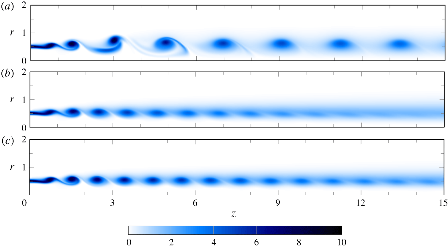
On the one hand,  $\boldsymbol{U}(r,z,t)$ represents the nonlinear axisymmetric unpaired flow that would occur without helical forcing at the jet inlet, such as displayed in figures 5(b,c). This flow, triggered by an axisymmetric harmonic (at frequency
 $\unicode[STIX]{x1D714}$) axial forcing at the inlet (plane
 $z=0$), is time-periodic. Details about the calculation of
 $\boldsymbol{U}$ are given in § 2.2.
On the other hand,  $\boldsymbol{u}^{\prime }(r,\unicode[STIX]{x1D703},z,t)$ represents the real non-axisymmetric perturbations of the flow owing to a prescribed non-axisymmetric inlet forcing. In the optimisation, we assume that
 $\boldsymbol{u}^{\prime }$ is the linear response to helical inlet forcing, with both
 $m=1$ and
 $m=-1$ components. By linearity, this implies that the perturbation is itself helical; we then introduce an
 $m=1$ complex part of the perturbation
 $\boldsymbol{u}_{\mathbf{1}}(r,z,t)$, such that
 $$\begin{eqnarray}\boldsymbol{u}^{\prime }(r,\unicode[STIX]{x1D703},z,t)=\boldsymbol{u}_{\boldsymbol{ 1}}(r,z,t)\text{e}^{\text{i}\unicode[STIX]{x1D703}}+\text{c.c.}=\boldsymbol{u}_{\boldsymbol{ 1}}(r,z,t)\text{e}^{\text{i}\unicode[STIX]{x1D703}}+\overline{\boldsymbol{u}}_{\boldsymbol{ 1}}(r,z,t)\text{e}^{-\text{i}\unicode[STIX]{x1D703}}.\end{eqnarray}$$
For bifurcating jets, it is required that the frequency of the helical forcing is half the frequency  $\unicode[STIX]{x1D714}_{f}$ of the axisymmetric forcing, as shown in § 1. Therefore, we can introduce the complex subharmonic helical inlet forcing functions
 $\boldsymbol{u}_{\mathbf{1}\boldsymbol{f},\mathbf{1}}(r)$ and
 $\boldsymbol{u}_{\mathbf{1}\boldsymbol{f},\mathbf{2}}(r)$ such that
 $$\begin{eqnarray}\boldsymbol{u}_{\mathbf{1}}(r,z=0,t)=\boldsymbol{u}_{\mathbf{1}\boldsymbol{f},\mathbf{1}}(r)\cos (\unicode[STIX]{x1D714}_{f}t/2)+\boldsymbol{u}_{\mathbf{1}\boldsymbol{f},\mathbf{2}}(r)\sin (\unicode[STIX]{x1D714}_{f}t/2),\quad \text{with}~\boldsymbol{u}_{\mathbf{1}\boldsymbol{f},\mathbf{1}}(r),\boldsymbol{u}_{\mathbf{1}\boldsymbol{f},\mathbf{2}}(r)\in \mathbb{C}^{3}.\end{eqnarray}$$
This is equivalent to prescribing a total real perturbation field  $\boldsymbol{u}^{\prime }(r,\unicode[STIX]{x1D703},z,t)$ equal to
 $$\begin{eqnarray}\displaystyle \boldsymbol{u}^{\prime }(r,\unicode[STIX]{x1D703},z=0,t) & = & \displaystyle 2\left[\text{Re}(\boldsymbol{u}_{\mathbf{1}\boldsymbol{f},\mathbf{1}})\cos (\unicode[STIX]{x1D703})\cos (\unicode[STIX]{x1D714}_{f}t/2)-\text{Im}(\boldsymbol{u}_{\mathbf{1}\boldsymbol{f},\mathbf{1}})\sin (\unicode[STIX]{x1D703})\cos (\unicode[STIX]{x1D714}_{f}t/2)\right.\nonumber\\ \displaystyle & & \displaystyle +\left.\text{Re}(\boldsymbol{u}_{\mathbf{1}\boldsymbol{f},\mathbf{2}})\cos (\unicode[STIX]{x1D703})\sin (\unicode[STIX]{x1D714}_{f}t/2)-\text{Im}(\boldsymbol{u}_{\mathbf{1}\boldsymbol{f},\mathbf{2}})\sin (\unicode[STIX]{x1D703})\sin (\unicode[STIX]{x1D714}_{f}t/2)\right]\!,\qquad\end{eqnarray}$$
where  $\text{Re}(\cdot )$ and
 $\text{Im}(\cdot )$ denote real and imaginary parts, respectively. Therefore, each forcing component has four functional real degrees of freedom, corresponding to two complex ones. More details on the optimisation are given in § 2.3.
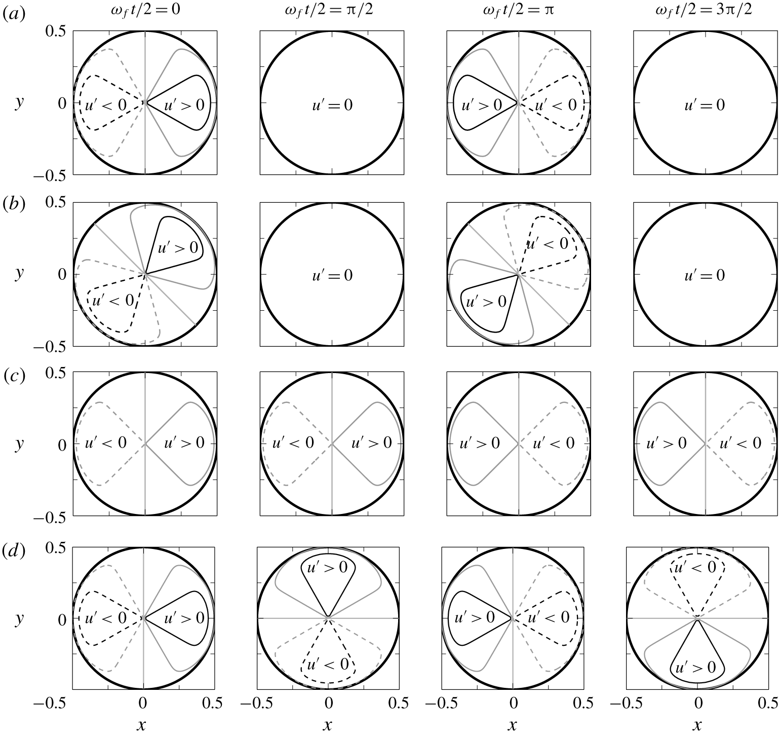
For a better understanding of such forcing, figure 4 represents some contours defined by isovalues of forcing that can be applied. We understand that when  $\boldsymbol{u}_{\mathbf{1}\boldsymbol{f},\mathbf{1}}$ and
 $\boldsymbol{u}_{\mathbf{1}\boldsymbol{f},\mathbf{2}}$ have a constant and equal phase, a constant symmetry axis in the inlet plane is introduced. This symmetry axis defines the bifurcating and bisecting planes. In the following, it will be found that such a constant phase condition is characteristic for the optimal forcing.
Examples of isovalues of perturbation fields in the inlet plane. Here  $U_{0}$ is defined in (2.6). (a)
 $u^{\prime }(r,\unicode[STIX]{x1D703},z=0,t)=U_{0}(r)\cos (\unicode[STIX]{x1D703})\cos (\unicode[STIX]{x1D714}_{f}t/2)$. In this case, a constant vertical symmetry plane is observed. (b)
 $u^{\prime }(r,\unicode[STIX]{x1D703},z=0,t)=U_{0}(r)(\cos (\unicode[STIX]{x1D703})+\sin (\unicode[STIX]{x1D703}))\cos (\unicode[STIX]{x1D714}_{f}t/2)/\sqrt{2}$, which can be simplified as
 $u^{\prime }(r,\unicode[STIX]{x1D703},z=0,t)=U_{0}(r)\cos (\unicode[STIX]{x1D703}-\unicode[STIX]{x03C0}/4)\cos (\unicode[STIX]{x1D714}_{f}t/2)$. Compared to figure 4(a), a
 $\unicode[STIX]{x03C0}/4$ azimuthal shift is introduced, shifting azimuthally the symmetry plane. (c)
 $u^{\prime }(r,\unicode[STIX]{x1D703},z=0,t)=U_{0}(r)\cos (\unicode[STIX]{x1D703})(\cos (\unicode[STIX]{x1D714}_{f}t/2)+\sin (\unicode[STIX]{x1D714}_{f}t/2))/\sqrt{2}$, which can be simplified as
 $u^{\prime }(r,\unicode[STIX]{x1D703},z=0,t)=U_{0}(r)\cos (\unicode[STIX]{x1D703})\cos (\unicode[STIX]{x1D714}_{f}t/2-\unicode[STIX]{x03C0}/4)$. Compared to figure 4(a), a
 $\unicode[STIX]{x03C0}/4$ time shift is introduced. The symmetry plane is left unchanged, constant in time. (d)
 $u^{\prime }(r,\unicode[STIX]{x1D703},z=0,t)=U_{0}(r)(\cos (\unicode[STIX]{x1D703})\cos (\unicode[STIX]{x1D714}_{f}t/2)+\sin (\unicode[STIX]{x1D703})\sin (\unicode[STIX]{x1D714}_{f}t/2))/\sqrt{2}$, which can be simplified as
 $u^{\prime }(r,\unicode[STIX]{x1D703},z=0,t)=U_{0}(r)\cos (\unicode[STIX]{x1D703}-\unicode[STIX]{x1D714}_{f}t/2)$. Compared to figure 4(a), the forcing is rotating in time. Hence, so does the symmetry plane.

2.2 Time-periodic base flow
2.2.1 Two different behaviours
Axisymmetric harmonic forcing at the nozzle of a laminar round jet excites, over a wide range of frequencies, a linear shear instability of the steady flow state, leading to exponential growth of the perturbation amplitude along the axial direction. As the amplitude reaches nonlinear levels, the shear layer rolls up into a regular street of vortex rings, which form and convect at the frequency of the applied forcing. Depending on flow parameters and forcing frequency, these vortices may undergo subsequent pairing (Hussain & Zaman Reference Hussain and Zaman1980; Zaman & Hussain Reference Zaman and Hussain1980; Ho & Huerre Reference Ho and Huerre1984; Shaabani-Ardali et al. Reference Shaabani-Ardali, Sipp and Lesshafft2019), and if the ambient flow is sufficiently quiet and the harmonic forcing is well-controlled, this pairing takes place in a perfectly regular fashion.
In cases where pairing occurs, two neighbouring vortices merge into one, such that the passage frequency of vortices downstream of the pairing location is exactly half that of the imposed forcing. If the forcing is characterised by the time period  $T_{f}$, such that
 $\unicode[STIX]{x1D714}_{f}=2\unicode[STIX]{x03C0}/T_{f}$, the ‘paired state’ is globally
 $2T_{f}$-periodic (
 $T_{f}$-periodic upstream of the pairing and
 $2T_{f}$-periodic downstream). An example of this behaviour, obtained by DNS, is shown in figure 5(a).
Vorticity snapshots of the periodic paired and unpaired states, obtained naturally for two different parameter settings. Simulation details, forcing amplitude, Reynolds and Strouhal numbers are defined in § 2.2.2. (a) Paired state ( $2T_{f}$-periodic) at
 $St=0.6$,
 $Re=2000$ and
 $A=5\,\%$ at
 $t=3T_{f}/2$. (b) Unpaired state (
 $T_{f}$-periodic) at
 $St=0.6$,
 $Re=1300$ and
 $A=5\,\%$ at
 $t=T_{f}/2$. (c) Unpaired stabilised state (
 $T_{f}$-periodic) at
 $St=0.6$,
 $Re=2000$ and
 $A=5\,\%$ at
 $t=T_{f}/2$.

Another case at different parameter settings, where no pairing is found to occur, is shown in figure 5(b). Vortices roll up close to the nozzle and advect downstream, until they are dissipated by viscosity. Such a flow state is (globally)  $T_{f}$-periodic and will be called hereafter an ‘unpaired state’.
It has been shown (Shaabani-Ardali et al. Reference Shaabani-Ardali, Sipp and Lesshafft2019) that the unpaired state exists for all parameter values, but that this state may be Floquet-unstable (Floquet Reference Floquet1883). In particular, it was found that, when unstable, the most unstable mode was always subharmonic at  $\unicode[STIX]{x1D714}_{f}/2$, leading after destabilisation to a paired state.
In the case of a bifurcating jet, none of the vortices undergo pairing, as shown in figures 1 and 2. In addition, the physical mechanism of Parekh et al. (Reference Parekh, Leonard and Reynolds1988) explains bifurcation by an alternating shifting of the ring vortices, which is achieved through helical forcing at half the vortex frequency. In the presence of pairing, paired vortices convect at the same frequency as the helical forcing, cancelling the alternating behaviour. Therefore, for the optimisation of the helical forcing, it is natural to seek an unpaired base flow, even if this flow may be unstable with respect to axisymmetric perturbations (Shaabani-Ardali et al. Reference Shaabani-Ardali, Sipp and Lesshafft2019). To do so, a simple stabilisation tool (Shaabani-Ardali, Sipp & Lesshafft Reference Shaabani-Ardali, Sipp and Lesshafft2017) is used to compute these unpaired states, which consists in adding a forcing term of the form
 $$\begin{eqnarray}\boldsymbol{f}=-\unicode[STIX]{x1D706}(\boldsymbol{U}(t)-\boldsymbol{U}(t-T_{f}))\end{eqnarray}$$
to the right-hand side of the Navier–Stokes equations (2.5). This allows to suppress  $2T_{f}$-periodic fluctuations on
 $T_{f}$-periodic dynamics. In this framework,
 $\unicode[STIX]{x1D706}$ is a forcing parameter that needs to be prescribed; an optimal value of
 $0.044\unicode[STIX]{x1D714}_{f}$ has been identified by Shaabani-Ardali et al. (Reference Shaabani-Ardali, Sipp and Lesshafft2017). In the same way as the selective frequency damping technique for steady flows (Åkervik et al. Reference Åkervik, Brandt, Henningson, Hœpffner, Marxen and Schlatter2006), the forcing term vanishes as the system converges towards a
 $T_{f}$-periodic unpaired state, such that the recovered state is a consistent solution of the unforced Navier–Stokes equations. The results of this technique are shown in figure 5(c), where the stabilised flow is plotted.
2.2.2 Configuration, governing equations and numerical discretisation
DNS were carried out using Nek5000, an incompressible spectral element code (Fischer et al. Reference Fischer, Kruse, Mullen, Tufo, Lottes and Kerkemeier2008). An axisymmetric laminar jet is described in cylindrical coordinates  $(z,r)$,
 $z$ being the main flow direction and
 $r$ being the radial distance from the jet axis. The flow is assumed to be governed by the incompressible Navier–Stokes equations with zero azimuthal velocity, written in dimensionless form as
 $$\begin{eqnarray}\frac{\unicode[STIX]{x2202}\boldsymbol{U}}{\unicode[STIX]{x2202}t}+(\boldsymbol{U}\boldsymbol{\cdot }\unicode[STIX]{x1D735})\boldsymbol{U}=-\unicode[STIX]{x1D735}P+\frac{1}{Re}\unicode[STIX]{x0394}\boldsymbol{U},\quad \unicode[STIX]{x1D735}\boldsymbol{\cdot }\boldsymbol{U}=0.\end{eqnarray}$$
The velocity  $\boldsymbol{U}$ has axial and radial components
 $U$ and
 $V$, and
 $P$ denotes pressure. The jet diameter
 $D$ and the inlet centreline velocity
 $\overline{U}$ are used to render the problem non-dimensional, defining the Reynolds number as
 $Re=\overline{U}D/\unicode[STIX]{x1D708}$, with
 $\unicode[STIX]{x1D708}$ the kinematic viscosity. The computational domain extends over
 $15\times 5$ diameters in the axial and radial directions, and it is discretised with 6600 spectral elements, each containing 64 mesh points. Boundary conditions are specified as follows.
(i) In the inlet plane,
 $z=0$, a hyperbolic-tangent velocity profile is imposed. In dimensionless form, its amplitude is modulated in time as (2.6)where$$\begin{eqnarray}\displaystyle \boldsymbol{U}(r,t) & = & \displaystyle \frac{1}{2}\left\{1-\tanh \left[\frac{1}{4\unicode[STIX]{x1D703}_{0}}\left(r-\frac{1}{4r}\right)\right]\right\}(1+A\cos (\unicode[STIX]{x1D714}_{f}t))\boldsymbol{e}_{\boldsymbol{z}}\nonumber\\ \displaystyle & = & \displaystyle U_{0}(r)(1+A\cos (\unicode[STIX]{x1D714}_{f}t))\boldsymbol{e}_{\boldsymbol{z}},\end{eqnarray}$$$A$ is the forcing amplitude of the jet, $\unicode[STIX]{x1D703}_{0}$ is the initial dimensionless mixing layer thickness and $\unicode[STIX]{x1D714}_{f}$ is the dimensional forcing frequency. The forcing period is given by $T_{f}=2\unicode[STIX]{x03C0}/\unicode[STIX]{x1D714}_{f}$, and the Strouhal number is defined as $St=\unicode[STIX]{x1D714}_{f}D/(2\unicode[STIX]{x03C0}\overline{U})$.
(ii) On the centreline of the jet,
$r=0$, axisymmetric boundary conditions are imposed, (2.7)$$\begin{eqnarray}\frac{\unicode[STIX]{x2202}U}{\unicode[STIX]{x2202}r}=V=\frac{\unicode[STIX]{x2202}P}{\unicode[STIX]{x2202}r}=0.\end{eqnarray}$$(iii) In the outlet plane,
$z=Z_{m}=15$, and on the outer radial boundary, $r=R_{m}=5$, a stress-free outflow condition is applied, (2.8)with$$\begin{eqnarray}-P\boldsymbol{n}+\frac{1}{Re}(\unicode[STIX]{x1D735}\boldsymbol{U})\boldsymbol{\cdot }\boldsymbol{n}=0,\end{eqnarray}$$$\boldsymbol{n}$ the normal vector at the boundary.


The flow configuration is thus characterised by the Reynolds number  $Re$, the Strouhal number
 $St$, the dimensionless mixing layer thickness
 $\unicode[STIX]{x1D703}_{0}$ and the forcing amplitude
 $A$. In this study, we keep the jet parameters fixed by considering a round jet at
 $Re=2000$ with a mixing layer thickness of
 $\unicode[STIX]{x1D703}_{0}=0.025$. The amplitude of the axisymmetric forcing is also kept fixed at
 $A=0.05$, whereas the forcing Strouhal number is varied. For all considered Strouhal numbers, convergence towards a periodic unpaired base state has been achieved. Shaabani-Ardali et al. (Reference Shaabani-Ardali, Sipp and Lesshafft2019) found that the band
 $0.5\leqslant St\leqslant 0.8$ is linearly unstable to subharmonic perturbations that lead to pairing; however, the time-delay feedback stabilisation in the present calculations successfully yields periodic unpaired base states over the entire considered range of Strouhal numbers.
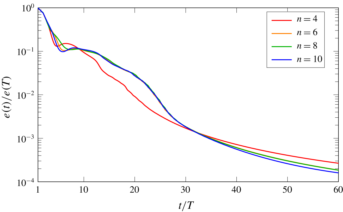
Numerical mesh convergence in these calculations, for the example case  $St=0.6$, is demonstrated in figure 6 by comparing the evolution of residuals in the stabilised computations for different spectral polynomial orders (
 $n=4$, 6, 8 and 10). A higher order is equivalent to a higher number of collocation points within each spectral element. The plotted quantity
 $e(t)$ in figure 6 is the norm of the difference between the flow states at time
 $t$ and at time
 $t-T_{f}$, as defined in Shaabani-Ardali et al. (Reference Shaabani-Ardali, Sipp and Lesshafft2017). It is seen that all orders yield the same convergence of the stabilisation routine; between resolutions
 $n\geqslant 6$, the flow states at each instant in the simulations are practically identical. The order
 $n=8$ is used in all following computations.
For different mesh resolutions (polynomial order  $n$ of individual spectral elements), the norm
 $e(t)$ of the residual difference between the flow velocity at time
 $t$ and time
 $t-T_{f}$ is traced as a function of
 $t$. These are the stabilised computations (with source term (2.4)) performed to find the periodic base flow at
 $Re=2000$ and
 $St=0.6$. The converged setting
 $n=8$ is used in the following.

2.3 Optimisation of the helical forcing
2.3.1 Equations governing helical perturbations
Before writing the linearised Navier–Stokes equations, the  $m=1$ perturbation field
 $(\boldsymbol{u}_{\mathbf{1}},p_{1})$ from (2.1) is rewritten as
 $(\boldsymbol{u}_{\mathbf{2}},p_{2})$ with
 $\boldsymbol{u}_{\mathbf{2}}=(u_{1,r},iu_{1,\unicode[STIX]{x1D703}},u_{1,z})^{t}$ and
 $p_{2}=p_{1}$ in order to remove imaginary coefficients. The linearised Navier–Stokes equations for the perturbation
 $(\boldsymbol{u}_{\mathbf{2}},p_{2})$ around the
 $T$-periodic base flow
 $\boldsymbol{U}(r,z,t)$ then read
 $$\begin{eqnarray}\displaystyle & \displaystyle \frac{1}{r}\frac{\unicode[STIX]{x2202}}{\unicode[STIX]{x2202}r}(ru_{2,r})+\frac{1}{r}u_{2,\unicode[STIX]{x1D703}}+\frac{\unicode[STIX]{x2202}u_{2,z}}{\unicode[STIX]{x2202}z}=0, & \displaystyle\end{eqnarray}$$
 $$\begin{eqnarray}\displaystyle & \displaystyle \frac{\unicode[STIX]{x2202}u_{2,r}}{\unicode[STIX]{x2202}t}+U_{r}\frac{\unicode[STIX]{x2202}u_{2,r}}{\unicode[STIX]{x2202}r}+u_{2,r}\frac{\unicode[STIX]{x2202}U_{r}}{\unicode[STIX]{x2202}r}+U_{z}\frac{\unicode[STIX]{x2202}u_{2,r}}{\unicode[STIX]{x2202}z}+u_{2,z}\frac{\unicode[STIX]{x2202}U_{r}}{\unicode[STIX]{x2202}z}=-\frac{\unicode[STIX]{x2202}p_{2}}{\unicode[STIX]{x2202}r}+\frac{1}{Re}\unicode[STIX]{x1D6E5}_{r}\boldsymbol{u}_{\mathbf{2}}, & \displaystyle\end{eqnarray}$$
 $$\begin{eqnarray}\displaystyle & \displaystyle \frac{\unicode[STIX]{x2202}u_{2,\unicode[STIX]{x1D703}}}{\unicode[STIX]{x2202}t}+U_{r}\frac{\unicode[STIX]{x2202}u_{2,\unicode[STIX]{x1D703}}}{\unicode[STIX]{x2202}r}+U_{z}\frac{\unicode[STIX]{x2202}u_{2,\unicode[STIX]{x1D703}}}{\unicode[STIX]{x2202}z}+\frac{U_{r}u_{2,\unicode[STIX]{x1D703}}}{r}=\frac{1}{r}p_{2}+\frac{1}{Re}\unicode[STIX]{x1D6E5}_{\unicode[STIX]{x1D703}}\boldsymbol{u}_{\mathbf{2}}, & \displaystyle\end{eqnarray}$$
 $$\begin{eqnarray}\displaystyle & \displaystyle \frac{\unicode[STIX]{x2202}u_{2,z}}{\unicode[STIX]{x2202}t}+U_{r}\frac{\unicode[STIX]{x2202}u_{2,z}}{\unicode[STIX]{x2202}r}+u_{2,r}\frac{\unicode[STIX]{x2202}U_{z}}{\unicode[STIX]{x2202}r}+U_{z}\frac{\unicode[STIX]{x2202}u_{2,z}}{\unicode[STIX]{x2202}z}+u_{2,z}\frac{\unicode[STIX]{x2202}U_{z}}{\unicode[STIX]{x2202}z}=-\frac{\unicode[STIX]{x2202}p_{2}}{\unicode[STIX]{x2202}z}+\frac{1}{Re}\unicode[STIX]{x1D6E5}_{z}\boldsymbol{u}_{\mathbf{2}}, & \displaystyle\end{eqnarray}$$
with the Laplacian in cylindrical coordinates
 $$\begin{eqnarray}\displaystyle & \displaystyle \unicode[STIX]{x1D6E5}_{r}\boldsymbol{u}_{\mathbf{2}}=\frac{1}{r}\frac{\unicode[STIX]{x2202}}{\unicode[STIX]{x2202}r}\left(r\frac{\unicode[STIX]{x2202}u_{2,r}}{\unicode[STIX]{x2202}r}\right)+\frac{\unicode[STIX]{x2202}^{2}u_{2,r}}{\unicode[STIX]{x2202}z^{2}}-\frac{2u_{2,r}}{r^{2}}-\frac{2u_{2,\unicode[STIX]{x1D703}}}{r^{2}}, & \displaystyle\end{eqnarray}$$
 $$\begin{eqnarray}\displaystyle & \displaystyle \unicode[STIX]{x1D6E5}_{\unicode[STIX]{x1D703}}\boldsymbol{u}_{\mathbf{2}}=\frac{1}{r}\frac{\unicode[STIX]{x2202}}{\unicode[STIX]{x2202}r}\left(r\frac{\unicode[STIX]{x2202}u_{2,\unicode[STIX]{x1D703}}}{\unicode[STIX]{x2202}r}\right)+\frac{\unicode[STIX]{x2202}^{2}u_{2,\unicode[STIX]{x1D703}}}{\unicode[STIX]{x2202}z^{2}}-\frac{2u_{2,\unicode[STIX]{x1D703}}}{r^{2}}-\frac{2u_{2,r}}{r^{2}}, & \displaystyle\end{eqnarray}$$
 $$\begin{eqnarray}\displaystyle & \displaystyle \unicode[STIX]{x1D6E5}_{z}\boldsymbol{u}_{\mathbf{2}}=\frac{1}{r}\frac{\unicode[STIX]{x2202}}{\unicode[STIX]{x2202}r}\left(r\frac{\unicode[STIX]{x2202}u_{2,z}}{\unicode[STIX]{x2202}r}\right)-\frac{u_{2,z}}{r^{2}}+\frac{\unicode[STIX]{x2202}^{2}u_{2,z}}{\unicode[STIX]{x2202}z^{2}}. & \displaystyle\end{eqnarray}$$
The following boundary and compatibility conditions are imposed:
 $$\begin{eqnarray}\displaystyle & \displaystyle \boldsymbol{u}_{\mathbf{2}}=\boldsymbol{u}_{\mathbf{2}\boldsymbol{f},\mathbf{1}}(r)\cos (\unicode[STIX]{x1D714}_{f}t/2)+\boldsymbol{u}_{\mathbf{2}\boldsymbol{f},\mathbf{2}}(r)\sin (\unicode[STIX]{x1D714}_{f}t/2)\quad \text{at}~z=0, & \displaystyle\end{eqnarray}$$
 $$\begin{eqnarray}\displaystyle & \displaystyle \frac{\unicode[STIX]{x2202}u_{2,r}}{\unicode[STIX]{x2202}r}=\frac{\unicode[STIX]{x2202}u_{2,\unicode[STIX]{x1D703}}}{\unicode[STIX]{x2202}r}=u_{2,z}=0\quad \text{at}~r=0, & \displaystyle\end{eqnarray}$$
 $$\begin{eqnarray}\displaystyle & \displaystyle u_{2,r}+u_{2,\unicode[STIX]{x1D703}}=0\quad \text{at}~r=0, & \displaystyle\end{eqnarray}$$
 $$\begin{eqnarray}\displaystyle & \displaystyle \frac{1}{Re}\frac{\unicode[STIX]{x2202}u_{2,r}}{\unicode[STIX]{x2202}r}-p=\frac{\unicode[STIX]{x2202}u_{2,\unicode[STIX]{x1D703}}}{\unicode[STIX]{x2202}r}=\frac{\unicode[STIX]{x2202}u_{2,z}}{\unicode[STIX]{x2202}r}=0\quad \text{at}~r=R_{m}, & \displaystyle\end{eqnarray}$$
 $$\begin{eqnarray}\displaystyle & \displaystyle \frac{1}{Re}\frac{\unicode[STIX]{x2202}u_{2,z}}{\unicode[STIX]{x2202}z}-p=\frac{\unicode[STIX]{x2202}u_{2,r}}{\unicode[STIX]{x2202}z}=\frac{\unicode[STIX]{x2202}u_{2,\unicode[STIX]{x1D703}}}{\unicode[STIX]{x2202}z}=0\quad \text{at}~z=Z_{m}, & \displaystyle\end{eqnarray}$$
with  $\boldsymbol{u}_{\mathbf{2}\boldsymbol{f},\mathbf{1}}$ and
 $\boldsymbol{u}_{\mathbf{2}\boldsymbol{f},\mathbf{2}}$ the corresponding inlet forcing modified from
 $\boldsymbol{u}_{\mathbf{1}\boldsymbol{f},\mathbf{1}}$ and
 $\boldsymbol{u}_{\mathbf{1}\boldsymbol{f},\mathbf{2}}$. In this new formalism, equations for
 $\boldsymbol{u}_{\mathbf{2}}$ only involve real coefficients, which is much more convenient for our numerical computations. The stress-free conditions (2.19), (2.20), consistent with the Nek5000 boundary treatment (2.8), arise as the ‘natural boundary conditions’ (see § 10.2.4 in Dick Reference Dick and Wendt2009) in this finite-element formulation. Their quality as non-reflecting outflow conditions have been examined by Theofilis (Reference Theofilis2017) and by Lesshafft (Reference Lesshafft2018).
2.3.2 Optimisation procedure
We aim to find the optimal inlet forcing that maximally shifts the vortices off the axis, at a given optimisation time  $T_{o}$, per unit input energy. Formally, we want to solve
 $$\begin{eqnarray}\max _{\Vert \boldsymbol{u}^{\prime }(r,\unicode[STIX]{x1D703},z=0,t)\Vert _{f}=1}\Vert \boldsymbol{u}^{\prime }(r,\unicode[STIX]{x1D703},z,t=T_{o})\Vert ,\end{eqnarray}$$
with  $T_{o}\longrightarrow \infty$. Again, the forcing
 $\boldsymbol{u}^{\prime }(r,\unicode[STIX]{x1D703},z=0,t)$ is assumed periodic with frequency
 $\unicode[STIX]{x1D714}_{f}/2$ (see (2.3)). The different norms used for forcing and response are detailed in § 2.4.
As will be demonstrated in § 3, this problem is well-posed, because the response converges towards an  $\unicode[STIX]{x1D714}_{f}/2$-periodic limit cycle when
 $T_{o}\longrightarrow \infty$. This shows that the base flow is stable with respect to
 $m=1$ subharmonic perturbations.
If the base flow were steady, the forced equations for linear perturbations could be written as
 $$\begin{eqnarray}\frac{\unicode[STIX]{x2202}\boldsymbol{u}^{\prime }}{\unicode[STIX]{x2202}t}=L\boldsymbol{u}+\hat{f}\text{e}^{\text{i}\unicode[STIX]{x1D714}t},\end{eqnarray}$$
which would lead to a traditional resolvent analysis (Schmid Reference Schmid2007). As in our case  $L$ depends on
 $t$, this type of analysis is not possible. However, several algorithms are available for the problem at hand.
First, a classical direct-adjoint algorithm, already employed for periodic-flow optimal perturbation analysis by Blackburn, Sherwin & Barkley (Reference Blackburn, Sherwin and Barkley2008), can be used. However, in the present optimisation, the flow perturbation field  $\boldsymbol{u}_{\mathbf{2}}$ is two-dimensional, whereas the prescribed inlet forcing distributions
 $\boldsymbol{u}_{\mathbf{2}\boldsymbol{f},\mathbf{1}}(r)$ and
 $\boldsymbol{u}_{\mathbf{2}\boldsymbol{f},\mathbf{2}}(r)$ are only one-dimensional. Therefore, if a direct-adjoint calculation is carried out, the adjoint field eventually needs to be projected on the one-dimensional inlet, and extra care needs to be taken to ensure that this is done properly (see Boujo & Gallaire Reference Boujo and Gallaire2015).
Another technique relies on the decomposition of the linearised operator, the forcing and response into Fourier components, and to solve the equations in Fourier space, as it is done in harmonic-balance methods. This has not been attempted here because of the considerable changes needed in the code compared with a standard time-stepping method, and because of the strong stiffness of these Newton-like problems.
In this work, the optimisation is carried out through a classical direct time-marching scheme detailed in § 2.3.3. A basis of forcing functions is chosen and each individual basis function is advanced in time. As the forcing only varies along the single radial dimension, a 300-dimensional basis has been found to be sufficient for an accurate resolution of the forcing space. Once time-stepping is carried out, thanks to linearity, the optimal combination of all 300 forcing vectors is calculated. This technique has several advantages compared with the two mentioned previously.
First, because the time-stepping and the optimisation are uncoupled in this process, many optimisation parameters, such as the final time  $T_{o}$, the norm chosen for the optimisation or other norm-related parameters, do not need to be fixed beforehand. These can be adjusted afterwards with the time-stepping results in order to check the dependence on these technical parameters. Changes in these hyper-parameters can be made almost for free.
Second, in our case the time-marching relies on an implicit scheme based on matrix inversions (see § 2.3.3); as the base flow changes in time, the matrix needs to be recalculated at every time step, requiring a significant computational effort. Therefore, time-marching  $N\gg 1$ vectors simultaneously, instead of one at a time for direct-adjoint optimisation, saves computational time. In addition, our approach removes the need to compute the adjoint part, thereby saving additional time.
Finally, compared with harmonic-balance techniques, which only capture the infinite time-horizon behaviour, our technique also allows to resolve transient dynamics.
2.3.3 Implementation
The evolution of the perturbation equations defined in § 2.3.1 is calculated using a fully implicit finite-difference time-stepping scheme of second order, implemented in the finite-element solver FreeFem++ (Hecht Reference Hecht2012). The mesh has the same size and resolution as that used in the Nek5000 calculations. We use  $P2$ finite elements for the velocity perturbation, whereas
 $P1$ finite elements are used for the pressure.
Once time-stepping is completed, the calculation of the optimal forcing combination can be done easily with Octave/Matlab routines. The resulting optimal forcing and response fields from this combination can then be obtained in FreeFem++.
This study is carried out for 10 values of the Strouhal number, between 0.35 and 0.8 in increments of 0.05, at a Reynolds number of 2000.
2.4 Forcing and response norms
In (2.21), the norms used for the forcing and for the response need to be specified. For the forcing, we consider the energy ( ${\mathcal{L}}_{2}$) norm, whereas for the response, two norms are introduced: the energy (
 ${\mathcal{L}}_{2}$) norm, and a norm based on the displacement of vortices.
Before going any further, let us recall some notation of scalar products. The scalar product of two real numbers  $x_{1}$,
 $x_{2}$ reads
 $\langle x_{1},x_{2}\rangle =x_{1}x_{2}$. The scalar product of two complex numbers
 $z_{1}$ and
 $z_{2}$ is defined as
 $\langle z_{1},z_{2}\rangle =\overline{z_{1}}z_{2}$. Subsequently, if
 $\boldsymbol{a}=(a_{i})_{i}$ and
 $\boldsymbol{b}=(b_{i})_{i}$ are two vectors represented in an orthonormal basis, their scalar product is
 $\langle \boldsymbol{a},\boldsymbol{b}\rangle =\sum _{i}\langle a_{i},b_{i}\rangle$. In the following,
 $\boldsymbol{u}^{\prime }$ and
 $\boldsymbol{v}^{\prime }$ are real vectors corresponding to real perturbation fields, whereas
 $\boldsymbol{u}_{\mathbf{2}}$ and
 $\boldsymbol{v}_{\mathbf{2}}$ are complex vectors corresponding to the helical mode
 $m=1$.
2.4.1 ${\mathcal{L}}_{2}$ norm for the forcing

For the forcing  $\boldsymbol{u}^{\prime }$, the standard
 ${\mathcal{L}}_{2}$ energy norm is used. This norm is derived from the following scalar product, which involves an integration over an entire subharmonic forcing period
 $2T_{f}$:
 $$\begin{eqnarray}\displaystyle \langle \boldsymbol{u}^{\prime },\boldsymbol{v}^{\prime }\rangle _{f} & = & \displaystyle \frac{1}{2T_{f}}\frac{1}{2\unicode[STIX]{x03C0}}\int _{0}^{2T_{f}}\!\int _{0}^{2\unicode[STIX]{x03C0}}\!\int _{0}^{R_{m}}r\langle \boldsymbol{u}^{\prime }(r,\unicode[STIX]{x1D703},z=0,t),\boldsymbol{v}^{\prime }(r,\unicode[STIX]{x1D703},z=0,t)\rangle \,\text{d}r\,\text{d}\unicode[STIX]{x1D703}\,\text{d}t,\qquad \quad\end{eqnarray}$$
 $$\begin{eqnarray}\displaystyle & = & \displaystyle \int _{0}^{R_{m}}r\left(\langle \text{Re}(\boldsymbol{u}_{\mathbf{2}\boldsymbol{f},\mathbf{1}}),\text{Re}(\boldsymbol{v}_{\mathbf{2}\boldsymbol{f},\mathbf{1}})\rangle +\langle \text{Im}(\boldsymbol{u}_{\mathbf{2}\boldsymbol{f},\mathbf{1}}),\text{Im}(\boldsymbol{v}_{\mathbf{2}\boldsymbol{f},\mathbf{1}})\rangle \right.\nonumber\\ \displaystyle & & \displaystyle +\left.\langle \text{Re}(\boldsymbol{u}_{\mathbf{2}\boldsymbol{f},\mathbf{2}}),\text{Re}(\boldsymbol{v}_{\mathbf{2}\boldsymbol{f},\mathbf{2}})\rangle +\langle \text{Im}(\boldsymbol{u}_{\mathbf{2}\boldsymbol{f},\mathbf{2}}),\text{Im}(\boldsymbol{v}_{\mathbf{2}\boldsymbol{f},\mathbf{2}})\rangle \right)\text{d}r,\end{eqnarray}$$
 $$\begin{eqnarray}\displaystyle & = & \displaystyle \frac{1}{2}\int _{0}^{R_{m}}r(\langle \boldsymbol{u}_{\boldsymbol{ 2}\boldsymbol{f},\mathbf{1}},\boldsymbol{v}_{\mathbf{2}\boldsymbol{f},\mathbf{1}}\rangle +\langle \overline{\boldsymbol{u}_{\mathbf{2}\boldsymbol{f},\mathbf{1}}},\overline{\boldsymbol{v}_{\mathbf{2}\boldsymbol{f},\mathbf{1}}}\rangle +\langle \boldsymbol{u}_{\mathbf{2}\boldsymbol{f},\mathbf{2}},\boldsymbol{v}_{\mathbf{2}\boldsymbol{f},\mathbf{2}}\rangle +\langle \overline{\boldsymbol{u}_{\mathbf{2}\boldsymbol{f},\mathbf{2}}},\overline{\boldsymbol{v}_{\mathbf{2}\boldsymbol{f},\mathbf{2}}}\rangle )\,\text{d}r.\qquad \quad\end{eqnarray}$$
This scalar product is different from the standard scalar product for complex numbers. While this must be kept in mind during the optimisation process, the norm it induces for the forcing  $\boldsymbol{u}^{\prime }$ is the standard
 ${\mathcal{L}}_{2}$ norm:
 $$\begin{eqnarray}\Vert \boldsymbol{u}^{\prime }\Vert _{f}^{2}=\int _{0}^{R_{m}}r(\langle \boldsymbol{u}_{\mathbf{2}\boldsymbol{f},\mathbf{1}},\boldsymbol{u}_{\mathbf{2}\boldsymbol{f},\mathbf{1}}\rangle +\langle \boldsymbol{u}_{\mathbf{2}\boldsymbol{f},\mathbf{2}},\boldsymbol{u}_{\mathbf{2}\boldsymbol{f},\mathbf{2}}\rangle )\,\text{d}r.\end{eqnarray}$$
2.4.2 ${\mathcal{L}}_{2}$ norm for the flow response

For the response, one possible norm is the energy norm based on the scalar product
 $$\begin{eqnarray}\displaystyle & & \displaystyle \!\!\!\langle \boldsymbol{u}^{\prime }(T_{o}),\boldsymbol{v}^{\prime }(T_{o})\rangle _{2}\nonumber\\ \displaystyle & & \displaystyle \!\!\!\quad =\frac{1}{2}\frac{1}{2\unicode[STIX]{x03C0}}\int _{0}^{Z_{opt}}\int _{0}^{2\unicode[STIX]{x03C0}}\int _{0}^{R_{m}}r\langle \boldsymbol{u}^{\prime }(r,\unicode[STIX]{x1D703},z,T_{o}),\boldsymbol{v}^{\prime }(r,\unicode[STIX]{x1D703},z,T_{o})\rangle \,\text{d}r\,\text{d}\unicode[STIX]{x1D703}\,\text{d}z\nonumber\\ \displaystyle & & \displaystyle \!\!\!\quad =\int _{0}^{Z_{opt}}\int _{0}^{R_{m}}r(\langle \text{Re}(\boldsymbol{u}_{\mathbf{2}}),\text{Re}(\boldsymbol{v}_{\mathbf{2}})\rangle +\langle \text{Im}(\boldsymbol{u}_{\mathbf{2}}),\text{Im}(\boldsymbol{v}_{\mathbf{2}})\rangle )\,\text{d}r\,\text{d}z,\end{eqnarray}$$
 $$\begin{eqnarray}\displaystyle & & \displaystyle \!\!\!\quad =\frac{1}{2}\int _{0}^{Z_{opt}}\int _{0}^{R_{m}}r(\langle \boldsymbol{u}_{\boldsymbol{ 2}}(r,z,T_{o}),\boldsymbol{v}_{\mathbf{2}}(r,z,T_{o})\rangle +\langle \overline{\boldsymbol{u}_{\mathbf{2}}}(r,z,T_{o}),\overline{\boldsymbol{v}_{\mathbf{2}}}(r,z,T_{o})\rangle )\,\text{d}r\,\text{d}z.\qquad \quad\end{eqnarray}$$
As we are interested in the evolution of perturbations close to the inlet, this scalar product is calculated on a reduced domain  $(r,z)\in [0;R_{m}]\times [0;Z_{opt}]$. Unless specified otherwise, a value of
 $Z_{opt}=5$ is chosen in the following. The effect of this value is investigated in § 3.4.1. Once again, this scalar product is different from the standard scalar product for complex numbers. However, the corresponding
 ${\mathcal{L}}_{2}$ norm for the response remains the same,
 $$\begin{eqnarray}\Vert \boldsymbol{u}^{\prime }(T_{o})\Vert _{2}^{2}=\int _{0}^{Z_{opt}}\int _{0}^{R_{m}}r\langle \boldsymbol{u}_{\mathbf{2}}(r,z,T_{o}),\boldsymbol{u}_{\mathbf{2}}(r,z,T_{o})\rangle \,\text{d}r\,\text{d}z.\end{eqnarray}$$
Note that, for the response, both  ${\mathcal{L}}_{2}$ scalar product and norm are not integrated over a full forcing period since this would require to store every time-step of every response field: storage is only done once in every forcing period
 $T_{f}$. A zero time-shift with respect to the axisymmetric forcing is chosen:
 $T_{o}$ is taken as
 $2nT_{f}$, with
 $n\in \mathbb{N}$. The influence of this shift is investigated in § 3.4.4, and the influence of
 $n$ is discussed in § 3.4.5.
2.4.3 Displacement norm for response
The bifurcation scenario (Lee & Reynolds Reference Lee and Reynolds1985; Parekh et al. Reference Parekh, Leonard and Reynolds1988) relies on a slight tilt and shift of the vortices near the jet inlet. Therefore, in this section, we define an alternative norm that quantifies the displacement of vortices from their unperturbed position. The location of a given vortex  $i$ at
 $T_{o}$ in a
 $(r,z)$-plane, cut at an angle
 $\unicode[STIX]{x1D703}_{c}$, can be defined as the centroid of its vorticity
 $\unicode[STIX]{x1D714}_{\unicode[STIX]{x1D703}}$ along
 $\unicode[STIX]{x1D703}$
 $$\begin{eqnarray}\boldsymbol{x}_{i}(\unicode[STIX]{x1D703}_{c},T_{o})=\frac{\displaystyle \iint _{r,z\in \unicode[STIX]{x1D734}_{i}}r\unicode[STIX]{x1D714}_{\unicode[STIX]{x1D703}}(r,\unicode[STIX]{x1D703}_{c},z,T_{o})\boldsymbol{x}\,\text{d}r\,\text{d}z}{\displaystyle \iint _{r,z\in \unicode[STIX]{x1D734}_{i}}r\unicode[STIX]{x1D714}_{\unicode[STIX]{x1D703}}(r,\unicode[STIX]{x1D703}_{c},z,T_{o})\,\text{d}r\,\text{d}z},\end{eqnarray}$$
with  $\unicode[STIX]{x1D734}_{i}$ the domain of the
 $i\text{th}$ vortex. This domain is defined as the rectangle
 $(z,r)\in [Z_{i}-\unicode[STIX]{x1D6FF}_{z}/2;Z_{i}+\unicode[STIX]{x1D6FF}_{z}/2]\times [0;1]$, with
 $Z_{i}$ the axial component of the centroid of the
 $i\text{th}$ vortex and
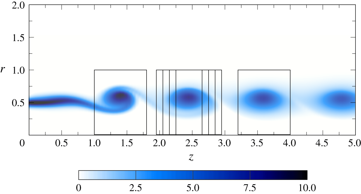
 $\unicode[STIX]{x1D6FF}_{z}$ conveniently fixed at 0.8. Examples of such boxes are represented in figure 7. The effect of
 $\unicode[STIX]{x1D6FF}_{z}$ on the optimisation is investigated in § 3.4.2.
Vorticity cut of the  $Re=2000$,
 $St=0.50$ base unpaired flow, with vortex domains represented for the first three vortices. For the second vortex, four
 $\unicode[STIX]{x1D6FF}_{z}$ sizes are sketched (0.4, 0.6, 0.8, 1.0), whereas for the first and third ones, only the
 $\unicode[STIX]{x1D6FF}_{z}=0.8$ box is represented.

The vorticity field  $\unicode[STIX]{x1D714}_{\unicode[STIX]{x1D703}}$ can be written as the sum of the vorticity
 $\unicode[STIX]{x1D6FA}_{\unicode[STIX]{x1D703}}$ induced by the base flow
 $\boldsymbol{U}(r,z,t)$ and an infinitesimal perturbation
 $\unicode[STIX]{x1D714}_{\unicode[STIX]{x1D703}}^{\prime }$ induced by the
 $m=1$ perturbation
 $\boldsymbol{u}^{\prime }$:
 $$\begin{eqnarray}\displaystyle \unicode[STIX]{x1D6FA}_{\unicode[STIX]{x1D703}}(r,z,t) & = & \displaystyle \frac{\unicode[STIX]{x2202}U_{r}}{\unicode[STIX]{x2202}z}-\frac{\unicode[STIX]{x2202}U_{z}}{\unicode[STIX]{x2202}r},\end{eqnarray}$$
 $$\begin{eqnarray}\displaystyle \unicode[STIX]{x1D714}_{\unicode[STIX]{x1D703}}^{\prime }(r,\unicode[STIX]{x1D703},z,t) & = & \displaystyle \frac{\unicode[STIX]{x2202}u_{r}^{\prime }}{\unicode[STIX]{x2202}z}-\frac{\unicode[STIX]{x2202}u_{z}^{\prime }}{\unicode[STIX]{x2202}r}\nonumber\\ \displaystyle & = & \displaystyle \left(\frac{\unicode[STIX]{x2202}u_{2,r}}{\unicode[STIX]{x2202}z}-\frac{\unicode[STIX]{x2202}u_{2,z}}{\unicode[STIX]{x2202}r}\right)\text{e}^{\text{i}\unicode[STIX]{x1D703}}+\text{c.c.}=\unicode[STIX]{x1D714}_{2,\unicode[STIX]{x1D703}}(r,z,t)\text{e}^{\text{i}\unicode[STIX]{x1D703}}+\text{c.c.}\end{eqnarray}$$
Specifying a perturbation amplitude  $\unicode[STIX]{x1D716}\ll 1$, we obtain
 $$\begin{eqnarray}\displaystyle \unicode[STIX]{x1D714}_{\unicode[STIX]{x1D703}}(r,\unicode[STIX]{x1D703},z,t) & = & \displaystyle \unicode[STIX]{x1D6FA}_{\unicode[STIX]{x1D703}}(r,z,t)+\unicode[STIX]{x1D716}\unicode[STIX]{x1D714}_{\unicode[STIX]{x1D703}}^{\prime }(r,\unicode[STIX]{x1D703},z,t),\end{eqnarray}$$
 $$\begin{eqnarray}\displaystyle & = & \displaystyle \unicode[STIX]{x1D6FA}_{\unicode[STIX]{x1D703}}(r,z,t)+\unicode[STIX]{x1D716}\unicode[STIX]{x1D714}_{2,\unicode[STIX]{x1D703}}(r,z,t)\text{e}^{\text{i}\unicode[STIX]{x1D703}}+\unicode[STIX]{x1D716}\overline{\unicode[STIX]{x1D714}_{2,\unicode[STIX]{x1D703}}}(r,z,t)\text{e}^{-\text{i}\unicode[STIX]{x1D703}}.\end{eqnarray}$$
The displacement norm with respect to the  $i\text{th}$ vortex
 $\unicode[STIX]{x1D734}_{i}$ can then be defined as
 $$\begin{eqnarray}\Vert \boldsymbol{u}^{\prime }(T_{o})\Vert _{disp,\unicode[STIX]{x1D734}_{i}}^{2}=\frac{1}{2}\frac{1}{2\unicode[STIX]{x03C0}}\int _{0}^{2\unicode[STIX]{x03C0}}\left\Vert \left.\frac{\text{d}\boldsymbol{x}_{i}(\unicode[STIX]{x1D703}_{c},T_{o})}{\text{d}\unicode[STIX]{x1D716}}\right|_{\unicode[STIX]{x1D716}=0}\right\Vert _{2}^{2}\text{d}\unicode[STIX]{x1D703}_{c}.\end{eqnarray}$$
For each vortex considered, it is possible to define a corresponding displacement norm. In the present study, following the bifurcation scenario (Parekh et al. Reference Parekh, Leonard and Reynolds1988), the displacement norm for the first three vortices is considered. Then, the axial position of the third vortex, depending on the Strouhal number, approximately corresponds to 5 jet diameters, which is consistent with the optimisation domain chosen for the  ${\mathcal{L}}_{2}$ norm (2.27). Full details on this norm are given in appendix A.
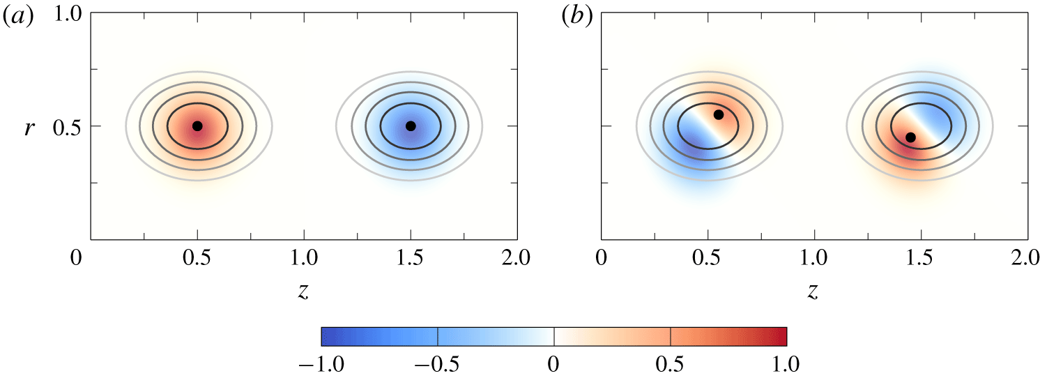
Note that the displacement norm is not strictly a norm but a semi-norm:  $\Vert \boldsymbol{u}^{\prime }(T_{o})\Vert _{disp,\unicode[STIX]{x1D734}_{i}}=0$ does not necessarily imply that
 $\boldsymbol{u}^{\prime }(T_{o})=\mathbf{0}$. As can be seen in appendix A and in figure 8, the displacement norm being equal to zero only implies that the vorticity centroid of the base flow and of the perturbation are at the same location. Therefore, the alternating pattern of figure 8(b) is a good candidate for a large displacement norm at fixed
 ${\mathcal{L}}_{2}$ norm. In this figure, one can easily understand that a large
 ${\mathcal{L}}_{2}$ norm does not necessarily imply a large displacement norm. Conversely, because the
 ${\mathcal{L}}_{2}$ norm is a true norm, a large displacement norm must imply a large
 ${\mathcal{L}}_{2}$ norm.
Schematic of base vortices (contour lines) superposed with a vorticity perturbation (colour field). The points represent the centroid of the superposition of the base flow and a finite-amplitude perturbation. (a) The perturbation does not change the centroid location, hence the displacement norm for this perturbation is zero. However, the perturbation is not identically zero, and neither is its  ${\mathcal{L}}_{2}$ norm. (b) The perturbation moves the centroid, and thus both norms are non-zero in this case.

Eventually, because of the definition of this norm that focuses on a given vortex  $i$, one displacement norm can be defined for each vortex ring. In our study, we assume the linear behaviour to be only valid in the vicinity of the inlet, where perturbations remain small; therefore, we only consider the displacement norm for each of the first three vortex rings.
2.5 Construction of a basis for the forcing
As explained in § 2.3.2, our purpose is to find the optimal forcing as the optimal linear combination of one-dimensional forcing functions. Both for convenience and for numerical accuracy, it is preferable to have a basis that is orthonormal with respect to the scalar product used for forcing (see § 2.4.1). This naturally suggests the use of Bessel functions, as the problem is formulated in cylindrical coordinates. As our problem is non-singular in  $r=0$, we choose Bessel functions of the first kind,
 $\text{J}_{k}$.
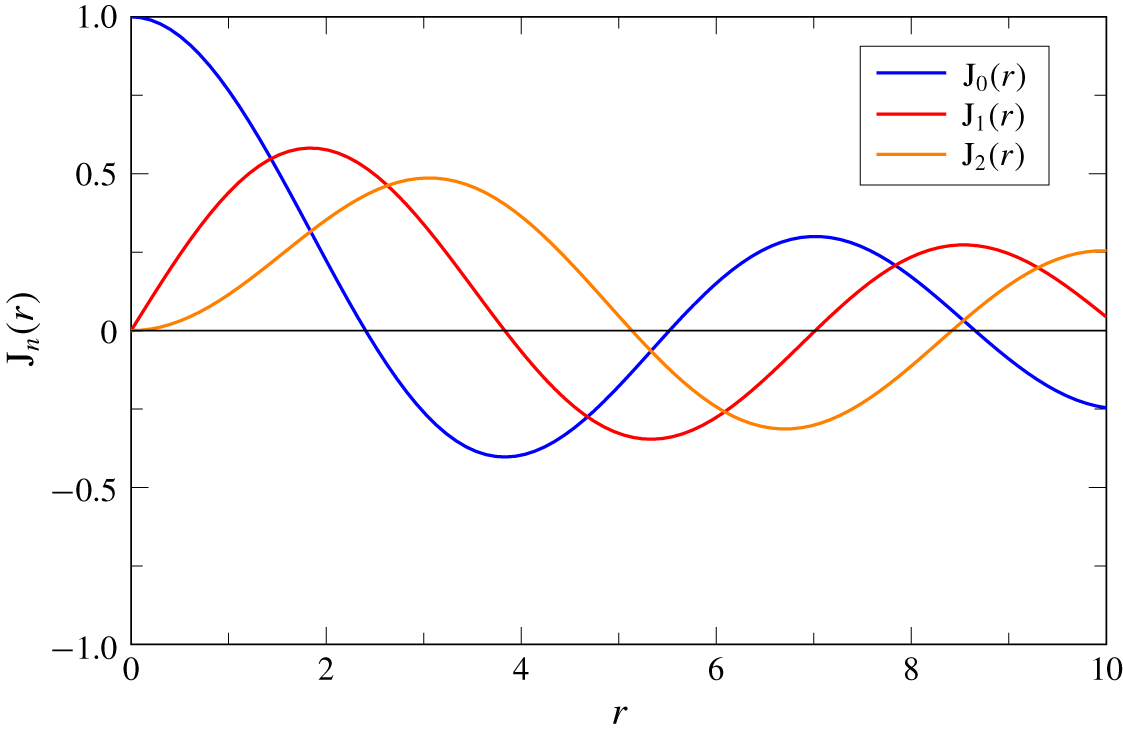
The Bessel functions  $\text{J}_{0}$,
 $\text{J}_{1}$ and
 $\text{J}_{2}$, plotted in figure 9, verify the properties (Abramowitz & Stegun Reference Abramowitz and Stegun1964)
 $$\begin{eqnarray}\text{J}_{0}(0)-1=\text{J}_{1}(0)=\text{J}_{2}(0)=\text{J}_{0}^{\prime }(0)=\text{J}_{2}^{\prime }(0)=0.\end{eqnarray}$$
Moreover, by denoting  $\unicode[STIX]{x1D706}_{i,n}$ the
 $n\text{th}$ root of
 $\text{J}_{i}$, these functions verify the orthogonality property
 $$\begin{eqnarray}\int _{0}^{1}r\text{J}_{i}(r\unicode[STIX]{x1D706}_{i,n})\,\text{J}_{i}(r\unicode[STIX]{x1D706}_{i,m})\,\text{d}r=\frac{\unicode[STIX]{x1D6FF}_{mn}}{2}[\text{J}_{i+1}(\unicode[STIX]{x1D706}_{i,n})]^{2}.\end{eqnarray}$$
Bessel functions of the first kind  $\text{J}_{0}$,
 $\text{J}_{1}$ and
 $\text{J}_{2}$.

We want to create a forcing basis that meets two criteria: first, it must be orthogonal, and second, all basis functions must verify the boundary conditions at  $r=0$ (2.17) and (2.18).
We consider the  $N$ first Bessel functions
 $\text{J}_{0}(r\unicode[STIX]{x1D706}_{0,m})$,
 $\text{J}_{1}(r\unicode[STIX]{x1D706}_{1,m})$ and
 $\text{J}_{2}(r\unicode[STIX]{x1D706}_{2,m})$,
 $1\leqslant m\leqslant N$, with which we can build a set of
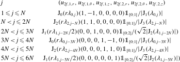
 $6N$ combined basis functions. These orthonormal basis functions are defined in table 1. For both radial and azimuthal forcing, a radial support over
 $0\leqslant r\leqslant 1$ is chosen, as their optimisation displayed in figure 13 reveals a quick decay after
 $r=0.5$ of these components; for the axial component, a support
 $0\leqslant r\leqslant 2$ is chosen, because its decay is slower.
Description of the orthonormal basis of forcing functions used in the optimisation. The indicator function  $\unicode[STIX]{x1D7D9}_{I}$, where
 $I$ is an interval, is 1 on
 $I$ and 0 elsewhere.

Any forcing function  $(\boldsymbol{u}_{2f,1},\boldsymbol{u}_{2f,2})$ can be projected onto this basis. Indeed, according to (2.17),
 $u_{2f,1,r}-u_{2f,1,\unicode[STIX]{x1D703}}$ and
 $u_{2f,2,r}-u_{2f,2,\unicode[STIX]{x1D703}}$ are functions with a zero derivative on the axis, and, by assuming that they have a compact support
 $[0;1]$, they can be decomposed into a
 $\text{J}_{0}(r\unicode[STIX]{x1D706}_{0,j})\unicode[STIX]{x1D7D9}_{[0;1]}$ series, where the indicator function
 $\unicode[STIX]{x1D7D9}_{[0;1]}$ is 1 on
 $[0;1]$ and 0 elsewhere.
Moreover, according to (2.17), (2.18),  $u_{2f,1,r}+u_{2f,1,\unicode[STIX]{x1D703}}$ and
 $u_{2f,2,r}+u_{2f,2,\unicode[STIX]{x1D703}}$ are functions with zero value and zero derivative on the axis. By assuming again that they have a compact support
 $[0;1]$, these can be decomposed into a
 $\text{J}_{2}(r\unicode[STIX]{x1D706}_{2,j})\unicode[STIX]{x1D7D9}_{[0;1]}$ series.
Finally, according to (2.17),  $u_{2f,1,z}$ and
 $u_{2f,2,z}$ have a zero value at
 $r=0$. By assuming a compact support
 $[0;2]$, they can be decomposed into a
 $\text{J}_{1}(r\unicode[STIX]{x1D706}_{1,j})\unicode[STIX]{x1D7D9}_{[0;2]}$ series. Further details of the optimisation procedure are given in appendix B.
3 Results of the optimisation
Throughout this section, except in § 3.4.5, the optimization time  $T_{o}$ used is chosen large enough such that the gain, forcing and response have reached their asymptotic values (
 $T_{o}\rightarrow \infty$).
3.1 Baseline case, $St=0.5$

In this subsection, the optimal  ${\mathcal{L}}_{2}$ norm long-term forcing and response for the case
 $Re=2000$ and
 $St=0.5$ are discussed. This particular set of parameters leads to particularly strong vortex spreading in bifurcating jets, according to previous studies (Parekh et al. Reference Parekh, Leonard and Reynolds1988; Tyliszczak & Geurts Reference Tyliszczak and Geurts2014; Gohil et al. Reference Gohil, Saha and Muralidhar2015; Gohil & Saha Reference Gohil and Saha2019).
It is shown in appendix B.1 that the forcing functions  $\boldsymbol{u}_{\mathbf{1}\boldsymbol{f},\mathbf{1}}(r)$ and
 $\boldsymbol{u}_{\mathbf{1}\boldsymbol{f},\mathbf{2}}(r)$ can be chosen real without loss of generality: prescribing complex values is equivalent to an azimuthal shift of the bifurcation plane. In this case, the forcing can be rewritten as
 $$\begin{eqnarray}\displaystyle \boldsymbol{u}_{\mathbf{2}}(r,z=0,t) & = & \displaystyle \boldsymbol{u}_{\mathbf{2}\boldsymbol{f},\mathbf{1}}(r)\cos (\unicode[STIX]{x1D714}_{f}t/2)+\boldsymbol{u}_{\mathbf{2}\boldsymbol{f},\mathbf{2}}(r)\sin (\unicode[STIX]{x1D714}_{f}t/2),\end{eqnarray}$$
 $$\begin{eqnarray}\displaystyle & = & \displaystyle |\boldsymbol{u}_{\mathbf{2}\boldsymbol{f}}(r)|\cos (\unicode[STIX]{x1D714}_{f}t/2+\text{arg}[\boldsymbol{u}_{\mathbf{2}\boldsymbol{f}}(r)]),\end{eqnarray}$$
where the cosine function is evaluated component-wise.
The functions  $|\boldsymbol{u}_{\mathbf{2}\boldsymbol{f}}(r)|$ and
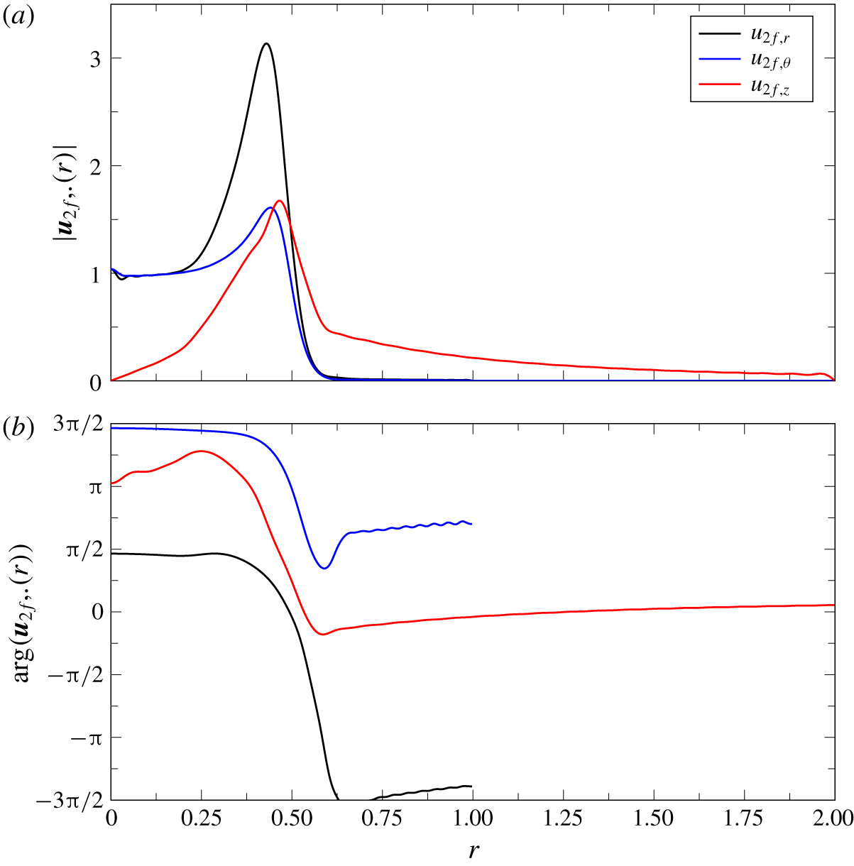
 $\text{arg}[\boldsymbol{u}_{\mathbf{2}\boldsymbol{f}}(r)]$ are displayed in figure 10. All three forcing components peak in the jet mixing layer, the most receptive region of jets (Ho & Huerre Reference Ho and Huerre1984). The dominant forcing component is radial. This shows that it is more effective to force in the radial, rather than in the axial or azimuthal direction, although axial forcing has been considered in most previous studies of jet bifurcation (Hilgers & Boersma Reference Hilgers and Boersma2001; Reynolds et al. Reference Reynolds, Parekh, Juvet and Lee2003; Tyliszczak & Geurts Reference Tyliszczak and Geurts2014). Concerning the phase, a phase shift in all three components is observed across the mixing layer. This phase shift is approximately equal to
 $\unicode[STIX]{x03C0}$ for
 $u_{2f,\unicode[STIX]{x1D703}}$,
 $2\unicode[STIX]{x03C0}$ for
 $u_{2f,r}$ and
 $\unicode[STIX]{x03C0}-3\unicode[STIX]{x03C0}/2$ for
 $u_{2f,z}$. This induces additional shear in the mixing layer, strengthening or weakening locally the vortex to be formed. Oscillations of small amplitude and small wavelength near the boundaries result from the truncated basis of Bessel functions.
The  ${\mathcal{L}}_{2}$ norm optimal forcing modulus and phase for
 $Re=2000$ and
 $St=0.50$. The phase was unwrapped to remain continuous in
 $r$. Here
 $|\boldsymbol{u}_{\mathbf{2}\boldsymbol{f}}(r)|$ and
 $\text{arg}(\boldsymbol{u}_{\mathbf{2}\boldsymbol{f}}(r))$ are defined in (3.2).

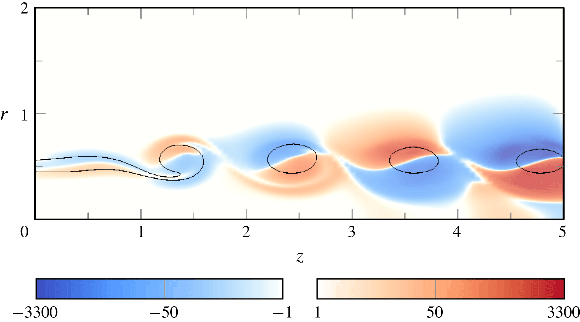
The optimal response, represented in figure 11, displays alternating positive and negative patches of vorticity. In the mixing layer, where the vortices are not yet formed, the positive and negative patches fit closely the mixing layer sides. When vortices have rolled up, the patches spread on either side of the formed vortex rings in an alternating fashion. The intensity of the patches grows exponentially with the axial distance  $z$. The contours of base flow vorticity show that the effect of these patches is to shift the vortex positions as expected. In an
 $(r,z)$ cut, two consecutive vortices are therefore sent in opposite directions. For a given vortex ring, two opposed points (separated by an azimuthal phase difference
 $\unicode[STIX]{x03C0}$), are sent in opposite
 $r$ and
 $z$ directions, because of the helical shape of the perturbation. As a consequence, in three dimensions, consecutive vortex rings are globally shifted off the axis in opposite directions.
The  ${\mathcal{L}}_{2}$ norm optimal vorticity response
 $\unicode[STIX]{x1D714}_{2,\unicode[STIX]{x1D703},opt}^{\prime }$ snapshot
 $Re=2000$ and
 $St=0.50$ at a zero phase. A level 4 contour of base flow vorticity has been added to understand the response pattern. A truncated and sign-sensitive logarithmic scale has been used.

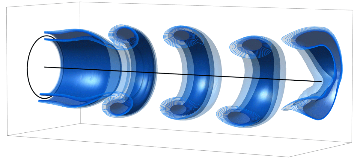
This is demonstrated in figure 12, where the axisymmetric unpaired base flow and the linear optimal  $m=1$ response are superposed. The vortices are alternatingly deflected towards the top and the bottom.
Snapshot of the superposition of the base flow and of the  ${\mathcal{L}}_{2}$-norm optimal response with a finite amplitude at
 $Re=2000$ and
 $St=0.5$.

The optimal and the first suboptimal gain values are calculated. The first suboptimal forcing mode, with its associated gain and response, are defined as the maximum-gain forcing in the subspace that is orthogonal to the optimal forcing. Although the gain value in itself does not have a clear meaning, because we compare a two-dimensional response with a one-dimensional forcing, the large optimal value  $1.01\times 10^{3}$ indicates a strong receptivity of the flow to this kind of forcing. The strong gain separation, the optimal gain being 102 times larger than the first suboptimal at
 $St=0.5$, indicates that only the leading forcing mode is relevant in this study; suboptimal forcing can only contribute marginally to the linear results.
3.2 Effect of the Strouhal number
In this section, we investigate the effect of the Strouhal number on optimisation results, obtained with respect to the  ${\mathcal{L}}_{2}$ norm.
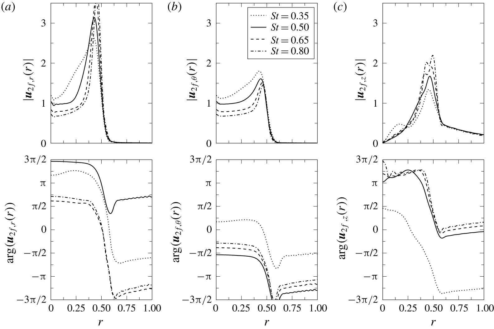
Figure 13 represents the optimal forcing shapes (modulus and phase of each component) for four different Strouhal numbers 0.35, 0.5, 0.65 and 0.8. A striking result is that the modulus shape is largely invariant with respect to the Strouhal number; however, the phase distributions vary greatly. In fact, this latter change can be understood as an overall shift of the phase functions: for each Strouhal number, the phase variations remain very similar, up to a constant shift.
Evolution of the  ${\mathcal{L}}_{2}$ norm optimal forcing modulus and phase for four different Strouhal numbers. Here
 $|\boldsymbol{u}_{\mathbf{2}\boldsymbol{f}}(r)|$ and
 $\text{arg}(\boldsymbol{u}_{\mathbf{2}\boldsymbol{f}}(r))$ are defined in (3.2).

In order to understand this shift quantitatively, we compare the values of two kinds of scalar products between optimal forcings. On the one hand, we compute the standard scalar product (2.25) for all Strouhal numbers; results are displayed in table 2(a). On the other hand, we calculate, for the four Strouhal numbers considered in figure 13, the scalar products between their forcing modulus, as displayed in table 2(b). This latter scalar product only accounts for differences in the modulus shape of the forcing, but not in the phase. By comparing these two results, it can be easily found that most of the changes with  $St$ are due to the phase difference, and not the shape difference. This is encouraging for practical applications of this method: if this optimal forcing shape were implemented in a physical device, it could work efficiently at different Strouhal numbers, by only varying the phase shift between forcing components.
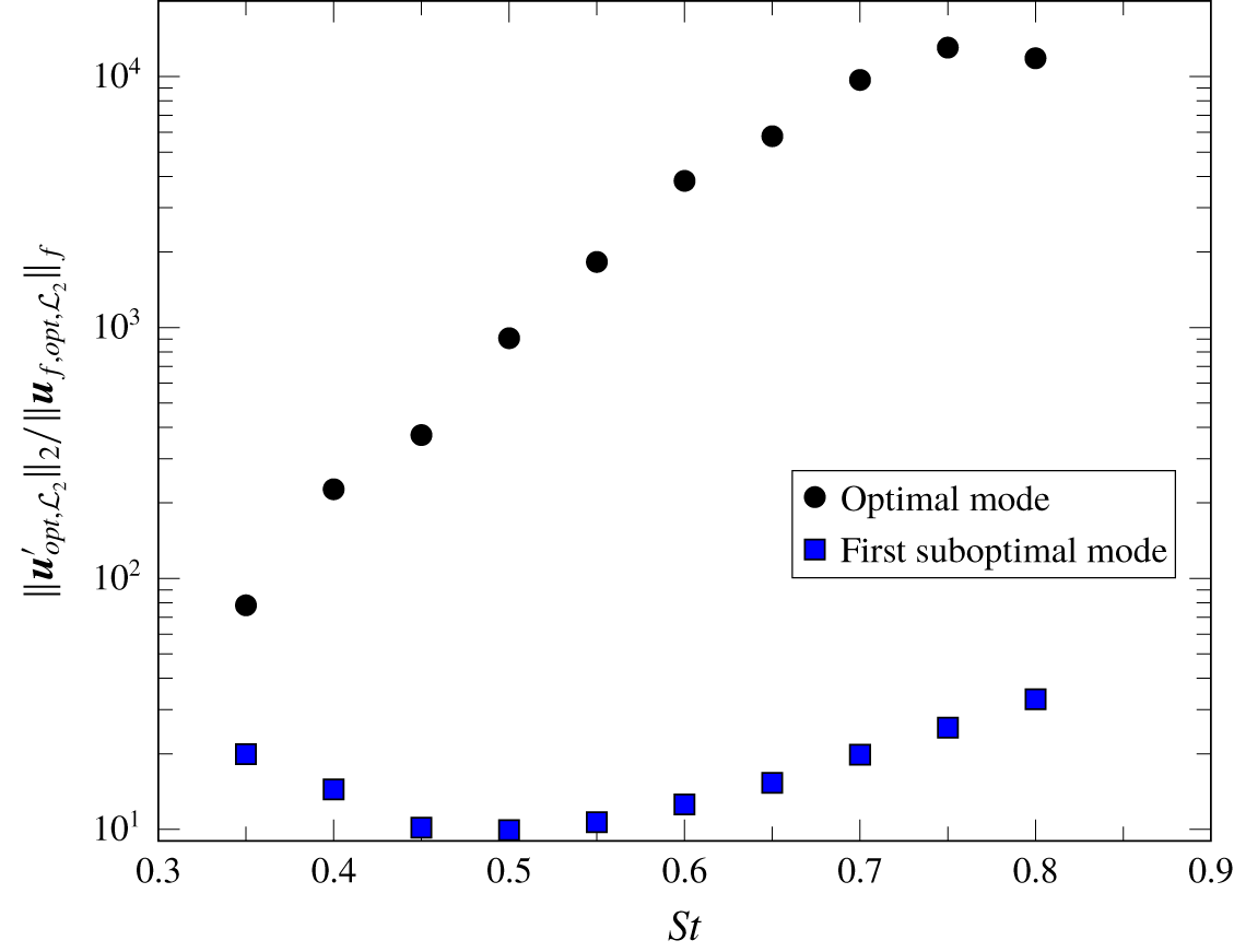
Evolution of the long-term ( $T_{o}\longrightarrow \infty$) optimal and first suboptimal gains for the
 ${\mathcal{L}}_{2}$ norm optimisation as a function of Strouhal number.

Comparison of  ${\mathcal{L}}_{2}$ norm optimal forcings and their modulus for different Strouhal numbers.

Optimal response shapes remain very similar at all Strouhal numbers to those represented in figure 11. However, it is difficult to derive precise quantitative comparisons of the responses, because these are located around base flow vortices, of which the position varies with Strouhal number.
The evolution of the optimal and first suboptimal gains as a function of the Strouhal number is represented in figure 14. Concerning the optimal gain, we observe large variations across Strouhal numbers, with an exponential growth as a function of  $St$ up to 0.75, where it seems to reach a saturation point. While previous studies (Danaila & Boersma Reference Danaila and Boersma1998, Reference Danaila and Boersma2000; da Silva & Métais Reference da Silva and Métais2002; Reynolds et al. Reference Reynolds, Parekh, Juvet and Lee2003; Tyliszczak & Boguslawski Reference Tyliszczak and Boguslawski2006, Reference Tyliszczak and Boguslawski2007; Gohil et al. Reference Gohil, Saha and Muralidhar2010; Gohil & Saha Reference Gohil and Saha2019) usually report bifurcation in the range
 $0.4\leqslant St\leqslant 0.6$, we find that the optimal gain continues to grow for Strouhal numbers greater than 0.6. This discrepancy between optimal and ad hoc forcing will be further investigated in the nonlinear regime (§ 4.3).
The suboptimal gain does not vary as much as the optimal, remaining of the order of 10 at all Strouhal numbers. Therefore, the gain separation largely increases with Strouhal number. Its consequences are further discussed in § 3.3.
3.3 Influence of the choice of norm
Two distinct response norms are used in this study: the  ${\mathcal{L}}_{2}$ norm, defined in § 2.4.2, and the displacement norm, defined in § 2.4.3. Only results for the
 ${\mathcal{L}}_{2}$ norm have been discussed so far. In this section, we investigate the influence of the norm by comparing optimisation results based on the
 ${\mathcal{L}}_{2}$ norm and the displacement norm of any of the first three vortex rings.
For  $St=0.5$, table 3 compares the forcing shapes in this case for the different norms used. The main conclusion is that, in this case, irrespective of the vortex choice for the displacement norm, the results are almost independent of the response norm used, with a minimal scalar product of 0.9838 between two different unit-norm forcing structures.
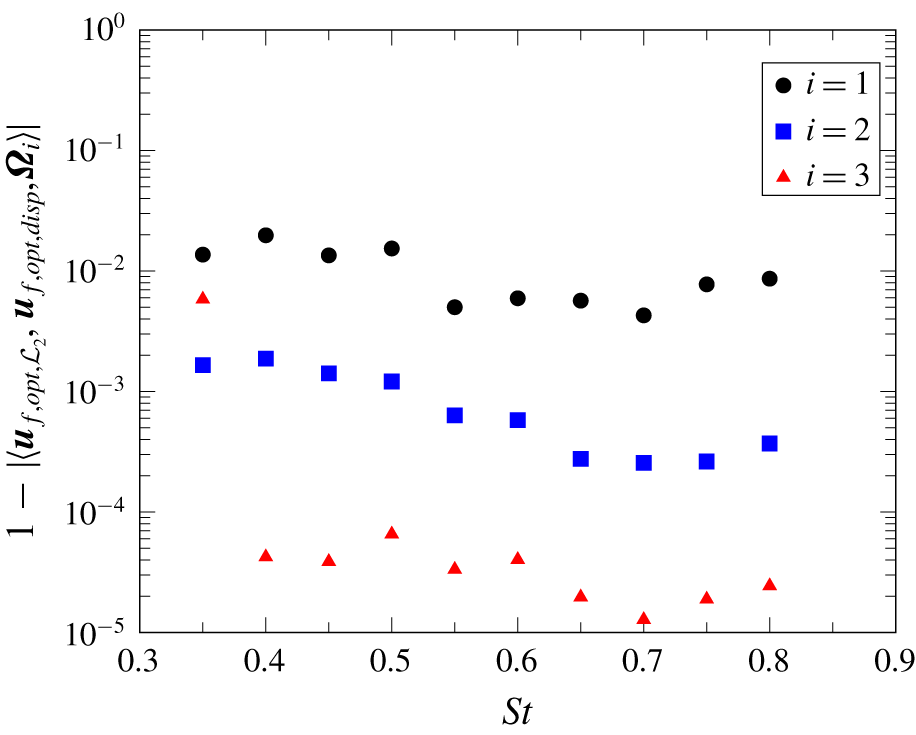
For every Strouhal number studied, scalar product between the optimal  ${\mathcal{L}}_{2}$ forcing and the optimal displacement norm forcings, for any of the first three vortices considered.

Scalar product between the optimal unit-norm forcings for the different norms considered. Here  $T_{o}=18$,
 $Re=2000$ and
 $St=0.5$.

For all Strouhal numbers, figure 15 compares the optimal  ${\mathcal{L}}_{2}$ forcing with optimal displacement norm forcing based on any of the first three vortices. Again, the results show an almost complete independence of the optimal forcing with respect to the chosen norm, with a minimal scalar product of 0.9802 between two different unit-norm forcings (for
 $St=0.4$). However, we see that the
 ${\mathcal{L}}_{2}$ norm results are closer to the results of the third vortex displacement; this can be understood with the exponential spatial growth of the optimal linear response (see § 3.1) that obviously puts a larger emphasis on the situation at the end of the optimisation domain, where the third vortex is approximately located.
The independence of the forcing norm can be explained by two main reasons. First, comparing figures 8 and 11, one sees that the optimal  ${\mathcal{L}}_{2}$ response shape, with its alternate pattern, is well-suited to shift the vortices off-axis, and therefore is well-suited for the displacement norm. Second, the large separation gains that exist between the optimal forcing and its suboptimals reinforces this phenomenon. Indeed, considering the
 ${\mathcal{L}}_{2}$ norm, figure 14 shows that the optimal gain is 3.9 times larger than the first suboptimal at
 $St=0.35$, and 513 times larger at
 $St=0.75$. Therefore, although the two norms considered do not measure the exact same quantities, the large gain separation balances this potential discrepancy. If the optimal
 ${\mathcal{L}}_{2}$ forcing has a much larger gain than any other orthogonal forcing, even though its corresponding unit-norm response shape might not shift the vortices optimally, this is compensated by its large gain.
3.4 Effect of simulation parameters
3.4.1 Length of the optimisation box for the energy norm
For the  ${\mathcal{L}}_{2}$ norm, the optimisation is carried out by calculating the response norm on the domain
 $0\leqslant r\leqslant R_{m}$ and
 $0\leqslant z\leqslant Z_{opt}$, with
 $Z_{opt}=5$. However, changing
 $Z_{opt}$ could change the results. In this section, we investigate the effect of changing
 $Z_{opt}$, in the
 $(Re=2000,~St=0.5)$ regime, by considering values of
 $Z_{opt}$ from 3 to 7.5 separated by 0.5 increments. When all the optimal forcings are calculated, scalar products between each couple of them are subsequently computed, and the most distant optimal forcings are those for
 $Z_{opt}=3$ and
 $Z_{opt}=7.5$, with a scalar product of 0.99961. The optimal forcing is thus independent of the domain length considered.
3.4.2 Length of the boxes around vortices for displacement norm
For the displacement norm, the optimal forcing is calculated by integrating perturbation quantities around the  $i\text{th}$ vortex core (
 $i=1$, 2 or 3). To perform this integration, a rectangular box
 $[Z_{i}-\unicode[STIX]{x1D6FF}_{z}/2;Z_{i}+\unicode[STIX]{x1D6FF}_{z}/2]\times [0;1]$, with
 $Z_{i}$ the axial position of the vortex (calculated as a centroid) and
 $\unicode[STIX]{x1D6FF}_{z}$ fixed to 0.8, is first chosen. However, the choice of
 $\unicode[STIX]{x1D6FF}_{z}$ could affect the results of the optimisation.
This effect is now studied for the  $Re=2000$ and
 $St=0.5$ case. Four different values of
 $\unicode[STIX]{x1D6FF}_{z}$ are tested: 0.4, 0.6, 0.8 and 1, as represented in figure 7. Above
 $\unicode[STIX]{x1D6FF}_{z}=1$, boxes for consecutive vortices would overlap. The first three vortices are considered here.
The results show that the optimal forcing barely depends on the box size: by considering scalar products between optimal forcing structures on the same vortex for different  $\unicode[STIX]{x1D6FF}_{z}$, all scalar products are above 0.992.
3.4.3 Effect of the dimension of the forcing space
The convergence of the optimal forcing shape with respect to the number  $N$ of basis functions is now evaluated. As these functions are orthonormal, the optimal forcing for a basis of dimension
 $N^{\prime }<N$ can easily be computed by taking the first
 $N^{\prime }$ components of the optimal
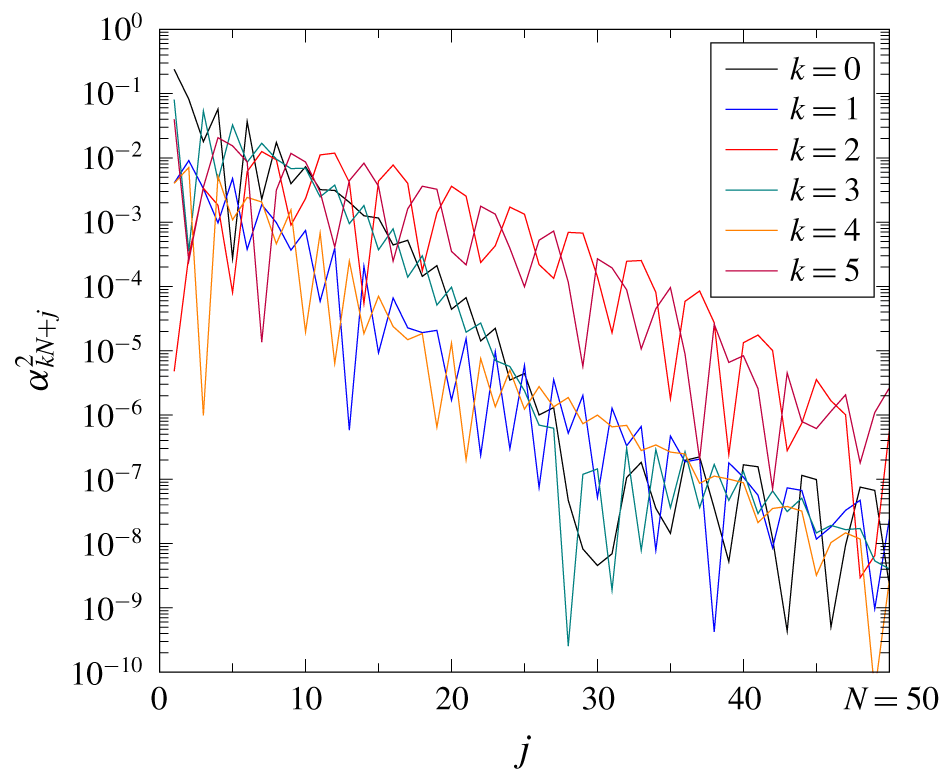
 $N$-forcing. Therefore, the evolution of energy component of the optimal forcing over each basis function, as represented in figure 16, shows the convergence of the algorithm as a function of
 $N$, for
 $Re=2000$ and
 $St=0.5$.
Energy component of the optimal forcing on each of the different basis forcing functions considered, for  $Re=2000$ and
 $St=0.50$. In this case,
 $N=50$.

It can be stated that the quickest mode to converge are the  $k=0$, 1, 3 and 4 modes, corresponding to forcing in the radial and azimuthal directions. However, in all cases, convergence is properly achieved, with energy levels contained in the last modes about 10 000 times lower than the ones in the first modes.
3.4.4 Effect of the time-shift with respect to the axisymmetric forcing
Our optimisation over a periodic flow is based on cost function evaluations only once per subharmonic cycle,  $T_{o}=2nT_{f}$. However, a large gain at these synchronized
 $T_{o}$ does not necessarily imply large gain for different
 $T_{o}=(2n+\unicode[STIX]{x1D711})T_{f}$ phase-shifted of
 $2\unicode[STIX]{x03C0}\unicode[STIX]{x1D711}$ with the fundamental forcing; in other words, there is no guarantee that a forcing that shifts well the vortices at a given objective time will not perform poorly at another time.
As a test, we evaluate the influence of a few optimisation time-shifts:  $\unicode[STIX]{x1D711}=0$ (phase 0), 1/4 (phase
 $\unicode[STIX]{x03C0}/2$), 1/2 (phase
 $\unicode[STIX]{x03C0}$) and 3/4 (phase
 $3\unicode[STIX]{x03C0}/2$). The different optimal
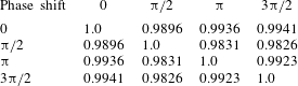
 ${\mathcal{L}}_{2}$-norm forcing functions found with these shifts are compared in table 4. Again, the optimal forcing is almost independent of the phase shift. This can be understood using the same arguments of the large gain separation as in § 3.3, but also physically by considering the jet bifurcation as a very receptive physical mechanism: in the interpretation of Parekh et al. (Reference Parekh, Leonard and Reynolds1988), the vortices are shed out of the axis, and they do not oscillate around a fixed equilibrium. Therefore, there is no chance that at a particular time-shift, the forcing has no effect on the vortices. If, at some time-step in the forcing period, the vortices are offset, then this offset continues through the entire cycle.
Scalar product of the  ${\mathcal{L}}_{2}$ norm optimal forcings for different phase shifts. Here
 $T_{o}=(2n+\unicode[STIX]{x1D711})T$ with
 $2n=18$ for phase 0 and 6 for others, with
 $Re=2000$ and
 $St=0.50$.

3.4.5 Final objective time $T_{o}$

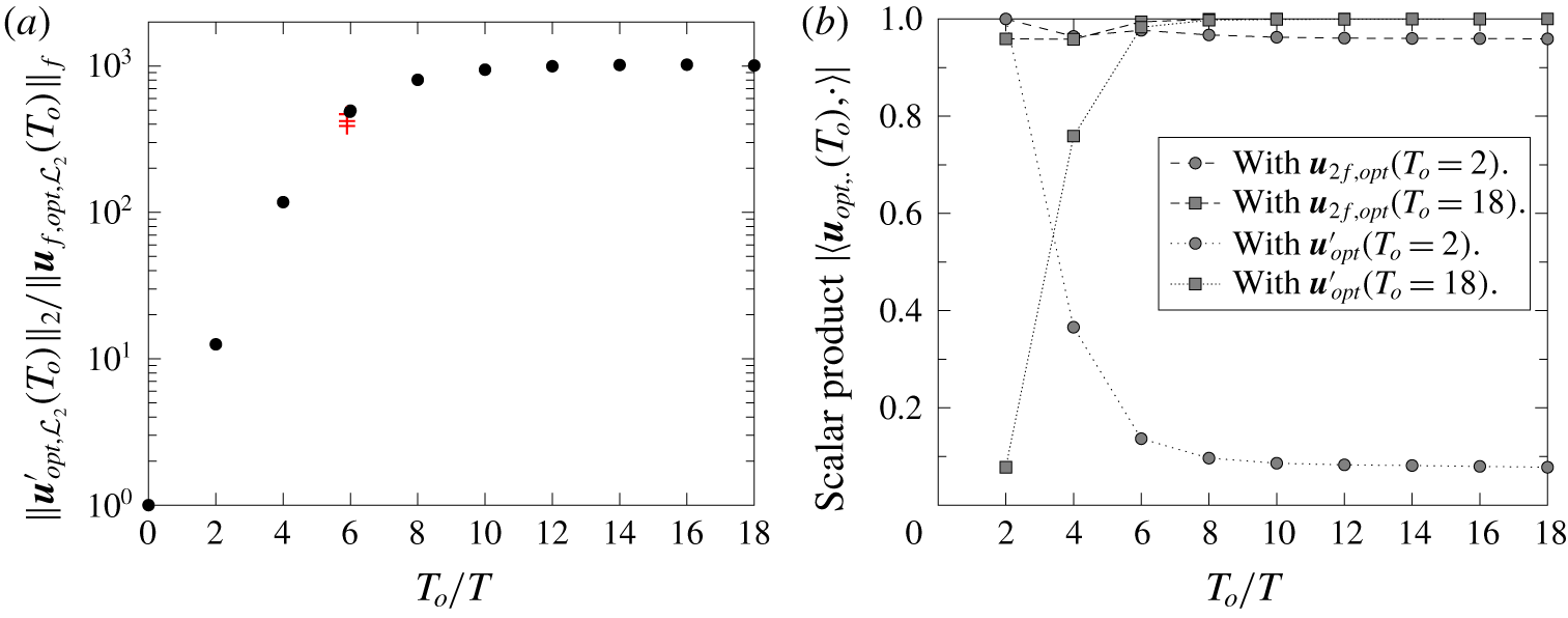
The optimal forcing and response can be calculated for different objective times  $T_{o}$. The shape of forcing functions and the associated gain evolves with time. At some point, the optimal forcing does not change and the gain reaches a plateau. In this study, the convergence condition we set for the final state is a variation of the gain by less than 0.5 % compared with the gain achieved two forcing periods before. In this section, we discuss the evolution of these quantities for the
 ${\mathcal{L}}_{2}$ norm and the
 $St=0.50$ case.
Figure 17(a) shows that, after an initial phase of exponential growth, the gain reaches a plateau. This confirms the stability of the axisymmetric unpaired base flow with respect to  $m=1$ perturbations.
Figure 17(b) displays the shape evolution with  $T_{o}$ of the optimal forcing and response by comparing each of these with the optimal quantities for
 $T_{o}=2$ and 18. Regarding forcing structures, little change occurs between
 $T_{o}=2$ and 18; the initial forcing is almost optimal, its shape is fixed. Therefore, if one is only interested in optimal forcing, there is no need to run the optimisation for long
 $T_{o}$. Concerning response structures, because of the spatial development of the perturbation field (more than two forcing periods are necessary to fill the five-diameter-long optimisation domain, because the initial perturbation is zero), the initial shape of the response, at
 $T_{o}=2$, has little resemblance with its final shape. After six forcing periods, they are almost identical.
The gain values obtained with different time shifts over six flow periods, as discussed in § 3.4.4, are shown as red crosses in figure 17(a). These values also give a measure of the moderate gain variations, within 12 % of their mean, that can be expected for time horizons in between integer multiples of the forcing period.
Evolution of optimal forcing, response and gain as a function of optimisation time  $T_{o}$ for the
 $Re=2000$,
 $St=0.50$ case. All quantities are optimised with respect to the
 ${\mathcal{L}}_{2}$ norm. (a) Evolution of the optimal gain. Black circles denote values obtained for the standard cases without phase shift between harmonic and subharmonic forcing, red crosses represent the gain obtained with the phase shifts discussed in § 3.4.4. (b) Evolution of the optimal forcing and response, with scalar product comparisons with
 $T_{o}=2$ and 18. The scalar products are all carried out over quantities normalized with respect to the relevant
 ${\mathcal{L}}_{2}$ norm.

3.5 Comparison with non-optimal ad hoc forcing
Previous studies (Danaila & Boersma Reference Danaila and Boersma1998, Reference Danaila and Boersma2000) prescribe an ad hoc helical forcing of the form
 $$\begin{eqnarray}\displaystyle \boldsymbol{u}(r,\unicode[STIX]{x1D703},z=0,t)=U_{0}(r)\left(1+A\cos (\unicode[STIX]{x1D714}_{f}t)+C\cos (\unicode[STIX]{x1D714}_{f}t/2+\unicode[STIX]{x1D719})\cos (\unicode[STIX]{x1D703})\left(\frac{2r}{D}\right)\right)\boldsymbol{e}_{\boldsymbol{z}},\quad & & \displaystyle\end{eqnarray}$$
with  $\unicode[STIX]{x1D719}$ the phase shift and
 $2r/D$ a factor imposed to enforce the compatibility condition (2.17) at
 $r=0$. In Parekh et al. (Reference Parekh, Leonard and Reynolds1988) and Danaila & Boersma (Reference Danaila and Boersma1998, Reference Danaila and Boersma2000), the phase shift
 $\unicode[STIX]{x1D719}$ is fixed at 0 to enforce simultaneous peaks (in time) of the axisymmetric and helical forcings.
The ad hoc forcing (3.3) is now compared with the optimal one. This comparison is made by calculating the scalar product between the two for four Strouhal number values 0.35, 0.5, 0.65 and 0.8. Results are summarized in table 5. Owing to the large gain separation shown in figure 14, these projection values approximately correspond to the ratio of the gains respectively achieved with ad hoc and optimal forcing, and it is seen that the increase of efficiency with the optimal forcing is significant.
Scalar product between normalised ad hoc forcing from (3.3) and optimal forcing with respect to the  ${\mathcal{L}}_{2}$ norm for four Strouhal number values.

4 Three-dimensional nonlinear results
In this section, the optimal forcing is implemented in three-dimensional nonlinear DNS. The purpose is to assess the performance of the optimised forcing across a large Strouhal number band, in comparison with an ad hoc forcing shape (3.3) that has been used in previous bifurcating jet studies.
4.1 Prescribed inflow forcing
In order to compare the effects of optimal versus ad hoc forcing in a meaningful way, a consistent normalisation of the input energy must be established. To this end, we calibrate the energy of helical forcing input with respect to the axisymmetric forcing (2.6). The latter is characterised by the fluctuation amplitude  $A$, and its energy is measured as
 $$\begin{eqnarray}\displaystyle \Vert \boldsymbol{U}\Vert _{f}^{2} & = & \displaystyle \frac{1}{2T_{f}}\frac{1}{2\unicode[STIX]{x03C0}}\int _{0}^{2T_{f}}\int _{0}^{2\unicode[STIX]{x03C0}}\int _{0}^{R_{m}}r\langle \boldsymbol{U}(r,\unicode[STIX]{x1D703},z=0,t),\boldsymbol{U}(r,\unicode[STIX]{x1D703},z=0,t)\rangle \,\text{d}r\,\text{d}\unicode[STIX]{x1D703}\,\text{d}t,\qquad\end{eqnarray}$$
 $$\begin{eqnarray}\displaystyle & = & \displaystyle \left(\int _{0}^{R_{m}}r\langle U_{0}(r)\boldsymbol{e}_{\boldsymbol{z}},U_{0}(r)\boldsymbol{e}_{\boldsymbol{z}}\rangle \,\text{d}r\right)\left(\frac{1}{2T_{f}}\int _{0}^{2T_{f}}(1+A\cos (\unicode[STIX]{x1D714}_{f}t))^{2}\text{d}t\right),\end{eqnarray}$$
 $$\begin{eqnarray}\displaystyle & = & \displaystyle \Vert U_{0}\boldsymbol{e}_{\boldsymbol{z}}\Vert _{f}^{2}\left(1+\frac{A^{2}}{2}\right),\end{eqnarray}$$
with  $R_{m}$ the outer radial boundary at the inlet in our simulations. Therefore, the energy of the base flow forcing is split between the mean component
 $\Vert U_{0}\boldsymbol{e}_{\boldsymbol{z}}\Vert _{f}^{2}$ and the axisymmetric forcing
 $A^{2}\Vert U_{0}\boldsymbol{e}_{\boldsymbol{z}}\Vert _{f}^{2}/2$.
4.1.1 Amplitude and phase of the optimal forcing
Adding the optimal helical forcing, with an amplitude of  $B\unicode[STIX]{x1D6E4}$, the jet inlet velocity (2.3) is prescribed as
 $$\begin{eqnarray}\displaystyle \boldsymbol{u}(r,\unicode[STIX]{x1D703},z=0,t) & = & \displaystyle U_{0}(r)(1+A\cos (\unicode[STIX]{x1D714}_{f}t))\boldsymbol{e}_{\boldsymbol{z}}\nonumber\\ \displaystyle & & \displaystyle +\,2B\unicode[STIX]{x1D6E4}\left[\text{Re}(\boldsymbol{u}_{\mathbf{1}\boldsymbol{f},\mathbf{1}})\cos (\unicode[STIX]{x1D703})\cos (\unicode[STIX]{x1D714}_{f}t/2)-\text{Im}(\boldsymbol{u}_{\mathbf{1}\boldsymbol{f},\mathbf{1}})\sin (\unicode[STIX]{x1D703})\cos (\unicode[STIX]{x1D714}_{f}t/2)\right.\nonumber\\ \displaystyle & & \displaystyle +\left.\text{Re}(\boldsymbol{u}_{\mathbf{1}\boldsymbol{f},\mathbf{2}})\cos (\unicode[STIX]{x1D703})\sin (\unicode[STIX]{x1D714}_{f}t/2)-\text{Im}(\boldsymbol{u}_{\mathbf{1}\boldsymbol{f},\mathbf{2}})\sin (\unicode[STIX]{x1D703})\sin (\unicode[STIX]{x1D714}_{f}t/2)\right]\!.\end{eqnarray}$$
A normalisation factor  $\unicode[STIX]{x1D6E4}$ is introduced, with a numerical value determined as 0.239 for the present flow case, such that the energy ratio between axisymmetric and helical forcing is given by
 $A^{2}/B^{2}$.
Without loss of generality, the azimuthal phase of the bifurcation plane is set to  $\unicode[STIX]{x1D703}=0$ by imposing all coefficients
 $u_{2f,\cdot ,\cdot }$ to be real-valued functions of
 $r$. This is possible because the perturbation equations for
 $\boldsymbol{u}_{\mathbf{2}}$ only involve real coefficients (see appendix B). Therefore, the total inflow forcing is finally recovered as
 $$\begin{eqnarray}\displaystyle \boldsymbol{u}(r,\unicode[STIX]{x1D703},0,t) & = & \displaystyle (1+A\cos (\unicode[STIX]{x1D714}_{f}t))U_{0}\boldsymbol{e}_{\boldsymbol{z}}\nonumber\\ \displaystyle & & \displaystyle +\,2B\unicode[STIX]{x1D6E4}\left[\begin{array}{@{}c@{}}(u_{2f,1,r}\cos (\unicode[STIX]{x1D714}_{f}t/2)+u_{2f,2,r}\sin (\unicode[STIX]{x1D714}_{f}t/2))\cos (\unicode[STIX]{x1D703})\\ (u_{2f,1,\unicode[STIX]{x1D703}}\cos (\unicode[STIX]{x1D714}_{f}t/2)+u_{2f,2,\unicode[STIX]{x1D703}}\sin (\unicode[STIX]{x1D714}_{f}t/2))\sin (\unicode[STIX]{x1D703})\\ (u_{2f,1,z}\cos (\unicode[STIX]{x1D714}_{f}t/2)+u_{2f,2,z}\sin (\unicode[STIX]{x1D714}_{f}t/2))\cos (\unicode[STIX]{x1D703})\end{array}\right].\end{eqnarray}$$
In this study, the amplitude  $B$ is fixed at 0.01, five times lower than the amplitude of the axisymmetric forcing prescribed; if this helical forcing had a constant shape in the radial direction harmonically modulated with time (as the axisymmetric), this would have corresponded to a maximum velocity amplitude with respect to the infinity norm of 1 % of the mean flow. This amplitude is much lower than what has been used in the literature: 5 % of the mean flow in Gohil et al. (Reference Gohil, Saha and Muralidhar2015), 1 % to 15 % in Tyliszczak & Geurts (Reference Tyliszczak and Geurts2014) or 15 % in Danaila & Boersma (Reference Danaila and Boersma1998, Reference Danaila and Boersma2000).
4.1.2 Amplitude of the ad hoc forcing
The simple, non-optimal helical forcing (3.3) is accordingly cast in normalised form as
 $$\begin{eqnarray}\displaystyle \boldsymbol{u}(r,\unicode[STIX]{x1D703},z=0,t)=U_{0}(r)\left(1+A\cos (\unicode[STIX]{x1D714}_{f}t)+B^{\prime }\unicode[STIX]{x1D6E4}^{\prime }\cos (\unicode[STIX]{x1D714}_{f}t/2)\cos (\unicode[STIX]{x1D703})\left(\frac{2r}{D}\right)\right)\boldsymbol{e}_{\boldsymbol{z}}, & & \displaystyle\end{eqnarray}$$
with a fixed zero-phase shift. A value  $\unicode[STIX]{x1D6E4}^{\prime }=1.850$ gives an energy ratio
 $A^{2}/B^{\prime 2}$ between axisymmetric and helical components, which is consistent with the above parametrisation of the optimal forcing. To enable fair comparisons,
 $B^{\prime }$ is fixed at 0.01, the same as
 $B$ in the previous section, and much lower than forcing levels commonly used in the literature.
4.2 Computational set-up
Nonlinear DNS are again carried out using Nek5000. In order to accommodate the spreading associated with bifurcation, a conical mesh is used, as represented in figure 18(a). The domain is 15 diameters long and its circular cross-section grows linearly from 5 jet diameters at the inlet plane ( $z=0$) to 16 diameters at the outlet plane (
 $z=15$). The mesh contains 27 720 spectral elements, each containing 8° of freedom in each direction; there are 30 elements in the axial direction and each
 $(x,y)$ plane contains 924 elements, as represented in the mesh cut in figure 18(b).
Mesh used for three-dimensional nonlinear computation.

The jet velocity is prescribed in the inlet plane according to either (4.5) or (4.6). An outflow condition (2.8) is applied at all other boundaries. In addition, the radial boundary downstream of  $z=5$ is padded with absorbing layers of thickness 1. This is necessary in order to ensure numerical stability in some cases of particularly strong jet spreading. As a consequence, the entire flow region
 $z>10$ is regarded as unphysical and is excluded from the following presentation of results.
A constant time step of  $\unicode[STIX]{x0394}t=2.5\times 10^{-3}$ is used throughout. The simulations are run for at least 100 dimensionless time units, in order to evacuate transient dynamics. Average quantities are then calculated over the last 10 forcing periods of the simulation.
4.3 Simulated jet bifurcation at various Strouhal numbers
Simulations are performed at  $Re=2000$, with Strouhal numbers ranging from 0.35 to 0.8, in increments of 0.05, with the optimal forcing (4.5). For comparison, the nonlinear response to ad hoc helical forcing (4.6) is computed for Strouhal numbers between 0.4 and 0.8, in increments of 0.1.
A vorticity snapshot of the optimally forced jet at  $Re=2000$ and
 $St=0.5$ is shown in figure 19(a). Close to the nozzle, axisymmetric vortex rings are seen to form rapidly, while the helical perturbation becomes appreciable about two jet diameters downstream of the inlet. The vortex rings are tilted and shifted off-axis, quickly resulting in bifurcation. In this process, the vortex rings are distorted on their inner side.
Comparing the nonlinear flow responses between optimised and ad hoc forcing in figures 19(a) and 19(b), we observe, without any ambiguity, that the optimal forcing leads to a much stronger and earlier bifurcation. In contrast to the optimised case, where the flow pattern is clearly symmetric with respect to the central plane, the effect of the simple forcing is too weak to enforce this symmetry.
Three-dimensional vorticity magnitude snapshots of the nonlinearly forced bifurcating jet for  $Re=2000$ and
 $St=0.5$. (a) The jet is forced optimally, (b) simple ad hoc forcing is applied.

The resulting time-averaged axial velocity is shown in figure 20. The symmetric bifurcation is clearly marked in the  $(x,z)$ plane, whereas the mean flow has entirely left the
 $(y,z)$ plane at a streamwise distance of about six diameters. All these results validate our optimisation procedure.
Mean axial velocity cut in the bifurcating ( $y=0$, a) and bisecting (
 $x=0$, b) planes for the
 $Re=2000$,
 $St=0.5$ case optimally forced with a 1 % amplitude. The sponge layers are not displayed.

Corresponding plots of the mean axial velocity in the bifurcation plane are shown in figure 21 for all Strouhal numbers. The response to optimal forcing is represented in the left and centre columns, alongside the response to ad hoc forcing in the right column. In addition, vorticity snapshots of the optimally forced jet for three different Strouhal numbers are displayed in figure 22.
Mean axial velocity cuts in the bifurcating plane for various values of the Strouhal number in the range  $[0.35;0.8]$ and for both optimal ((a,d,g,j,m) and (b,e,h,k,n)) and ad hoc (c,f,i,l,o) forcing. The forcing amplitude is fixed for
 $B$ and
 $B^{\prime }$ at 1 % and the colour bar can be found in figure 20. The sponge layers are not displayed.

Three-dimensional vorticity magnitude snapshots of the nonlinearly optimally forced bifurcating jet for  $Re=2000$ and three different Strouhal values: 0.35, 0.65 and 0.80.

In the optimally forced cases, a pronounced bifurcation is observed at all Strouhal numbers, despite the low helical forcing amplitude. Below  $St=0.55$, the cleavage between the two branches widens with the Strouhal number, which is fully consistent with the increase of the linear gain shown in figure 14. Below this threshold, vortices do not distort one another, as shown in figure 22(a): such an interaction only starts around
 $St=0.55$ (see figure 19a). Above this value, while the jet continues to display strong flaring, a third central structure emerges progressively, and the mean flow is increasingly mixed in between the paths of the outer jets. Depending on the Strouhal number, this central structure resembles either a large central jet (
 $St=0.75$ and 0.8), as shown in the mean flow cuts and in figure 22(c), or it resembles two smaller side jets (
 $St=0.6$, 0.65 and 0.7), as shown in the mean flow cuts and in figure 22(b). The occurrence of this central mixing seems to be linked to an observation by Parekh et al. (Reference Parekh, Leonard and Reynolds1988): at high Strouhal number, associated with small spatial separation, the vortex rings interact and distort one another more intensely. This purely nonlinear effect, confirmed in figure 22, also leads to a stronger transition to turbulence in our simulations. Even though it is not captured by the analysis in § 2, it provides a reasonable explanation for the blurring of the mean flow in the central region. However, the simulations clearly demonstrate that the continued exponential growth of the linear gain beyond
 $St=0.55$ is not reflected in the nonlinear flow behaviour.
The simple ad hoc helical forcing, as seen in the right column of figure 21, clearly is much less efficient in producing a bifurcation. The flaring, when it occurs, sets in further downstream, typically with less pronounced branch formation, and the loss of symmetry in the 10-period mean indicates a much reduced efficiency to alternatively deviate the jet. Second, a clear bifurcation within 10 diameters of the inlet is only observed in the narrow range  $0.4\leqslant St\leqslant 0.5$. Owing to the low helical forcing amplitude of 1 % in our simulations, this band of
 $St$ is consistent with the literature (Reynolds et al. Reference Reynolds, Parekh, Juvet and Lee2003; Tyliszczak & Geurts Reference Tyliszczak and Geurts2014). Conversely, optimised forcing results in bifurcation over the entire range of Strouhal numbers considered in this study.
Vortex pairing, as a subharmonic Floquet instability, is absent in all bifurcation simulations, even though the base flows in these calculations are Floquet-unstable over the Strouhal number range between 0.5 and 0.8 (see Shaabani-Ardali et al. Reference Shaabani-Ardali, Sipp and Lesshafft2019). The helical forcing is seen to be efficient at suppressing the vortex pairing instability.
5 Conclusion
Optimal forcing of jet bifurcation, as an example of forced symmetry breaking of a time-periodic base flow, has been investigated in a linear framework. Results have been validated in three-dimensional DNS calculations.
This study relies on the bifurcation scenario originally described by Lee & Reynolds (Reference Lee and Reynolds1985) and Parekh et al. (Reference Parekh, Leonard and Reynolds1988). Following their physical description, we have proposed to optimise the bifurcating jet by maximising a linear helical perturbation of an array of axisymmetric ring vortices in a jet. To suppress the pairing instability, the axisymmetric unpaired base flow has been computed through a time-delayed feedback technique (Shaabani-Ardali et al. Reference Shaabani-Ardali, Sipp and Lesshafft2017). Then, the optimisation framework has been derived, with two maximisation norms introduced: the classical  ${\mathcal{L}}_{2}$ norm and a norm based on vortex displacement. Numerically, this optimisation is performed through time-stepping of a basis of one-dimensional inlet forcing functions and the selection of their optimal linear combination.
After carrying out the optimisation, it has been found that irrespective of the Strouhal number, chosen between 0.35 and 0.8, one should mostly force around the mixing layer position and mainly along the radial direction, as opposed to axial velocity forcing, employed in most previous studies. By varying the Strouhal number, the shape of the modulus of the optimal forcing does not vary much, but it undergoes global shifts in phase. For practical applications, this shows that optimal perturbations can be easily provided by a unique setup along a large band of Strouhal numbers just by varying the phase difference with the axisymmetric forcing. Moreover, the identified optimal forcing is virtually universal: it is independent of both the norm and the hyperparameters chosen, such as the domain size or the time shift. This universality is explained by a large gain separation between the optimal and all suboptimal forcing: varying the optimisation parameters (norms, domain length) as well as the physical parameters (time horizon  $T_{o}$, phase difference of the chosen
 $T_{o}$, vortex chosen to optimise around) has little influence on the final result. The gain grows exponentially with Strouhal number, before saturating around
 $St=0.75$, and it is at least five times larger than that achieved with simple ad hoc forcing strategies.
Finally, three-dimensional DNS have been carried out to validate the results. A low forcing amplitude of 1 % has been chosen for the helical forcing. It has been found that the linear optimal forcing performs extremely well over the entire band of Strouhal numbers  $0.35\leqslant St\leqslant 0.8$, leading to a large flaring of the jet and, therefore, a large improvement of its mixing efficiency. Two kinds of flow topology have been found: for Strouhal values below 0.55, a classical bifurcating jet is obtained, whereas for Strouhal numbers above 0.55 a third central structure emerges. In all cases, comparisons with ad hoc forcing strategies show that the optimisation triggers bifurcation much more efficiently, by moving the bifurcation point upstream, and leading to a stronger displacement of vortices; further, that this triggering can occur over a very large Strouhal band, compared with the narrow band in which bifurcation is found for non-optimal forcing strategies.
Mathematically, in this study, we have derived a framework to carry out linear optimisation over periodic flows for long time horizons. Physically, our work provides a better understanding of the bifurcating jet phenomenon. Even though our study focuses on a laminar bifurcating jet at moderate Reynolds number, previous results (Tyliszczak & Geurts Reference Tyliszczak and Geurts2014) have shown that the turbulence level in bifurcating jets becomes important only when it exceeds the axisymmetric and helical forcings levels. This implies that an optimal forcing for a laminar flow would remain close-to-optimal for turbulent flows with a forcing amplitude adjusted so that it exceeds the turbulence level. Moreover, Parekh et al. (Reference Parekh, Leonard and Reynolds1988) have shown that jet bifurcation could be essentially triggered in similar ways both at moderate and large Reynolds numbers. Wu et al. (Reference Wu, Fan, Zhou, Li and Noack2018) identified jet bifurcation as the optimal way to increase mixing in a turbulent jet.
An interesting question, outside the scope of this study, would be to precisely understand the effect of turbulence and Reynolds number on our results. To do so, one could rely on a linear optimisation over the base flow of a turbulent phase-averaged axisymmetric pulsed jet. Such an analysis would transpose the resolvent framework to time-periodic (in an averaged sense) turbulent flows, and would be useful for many other situations.
Acknowledgements
We thank R. Yegavian for his help with the parallelisation of FreeFem++. This work was granted access to the HPC resources of TGCC under the allocation grant no. 2016-2a6451 made by GENCI, and it was financially supported by the Délégation Générale de l’Armement under grant no. 2015.60.0004.00.470.75.01.
Declaration of interests
The authors report no conflict of interest.
Appendix A. Details on the displacement norm
From (2.35), the displacement norm can be written as
 $$\begin{eqnarray}\Vert \boldsymbol{u}^{\prime }(T_{o})\Vert _{disp,\unicode[STIX]{x1D734}_{i}}^{2}=\frac{1}{2}\frac{1}{2\unicode[STIX]{x03C0}}\int _{0}^{2\unicode[STIX]{x03C0}}\left\Vert \left.\frac{\text{d}\boldsymbol{x}_{i}(\unicode[STIX]{x1D703}_{c},T_{o})}{\text{d}\unicode[STIX]{x1D716}}\right|_{\unicode[STIX]{x1D716}=0}\right\Vert _{2}^{2}\text{d}\unicode[STIX]{x1D703}_{c}.\end{eqnarray}$$
By introducing the original vortex position  $\boldsymbol{X}_{i}(T_{o})$ and the total vorticity of the
 $i\text{th}$ vortex
 $\unicode[STIX]{x1D6FA}_{i,tot}(T_{o})$,
 $$\begin{eqnarray}\displaystyle & \displaystyle \boldsymbol{X}_{i}(T_{o})=R_{i}(T_{o})\boldsymbol{e}_{\boldsymbol{r}}+Z_{i}(T_{o})\boldsymbol{e}_{\boldsymbol{z}}=\frac{\displaystyle \iint _{\unicode[STIX]{x1D734}_{i}}r\unicode[STIX]{x1D6FA}_{\unicode[STIX]{x1D703}}(r,z,T_{o})\boldsymbol{x}\,\text{d}r\,\text{d}z}{\displaystyle \iint _{\unicode[STIX]{x1D734}_{i}}r\unicode[STIX]{x1D6FA}_{\unicode[STIX]{x1D703}}(r,z,T_{o})\,\text{d}r\,\text{d}z}, & \displaystyle\end{eqnarray}$$
 $$\begin{eqnarray}\displaystyle & \displaystyle \unicode[STIX]{x1D6FA}_{i,tot}(T_{o})=\iint _{\unicode[STIX]{x1D734}_{i}}r\unicode[STIX]{x1D6FA}_{\unicode[STIX]{x1D703}}(r,z,T_{o})\,\text{d}r\,\text{d}z, & \displaystyle\end{eqnarray}$$
the displacement norm can be rewritten as
 $$\begin{eqnarray}\displaystyle & & \displaystyle \Vert \boldsymbol{u}^{\prime }(T_{o})\Vert _{disp,\unicode[STIX]{x1D734}_{i}}^{2}\nonumber\\ \displaystyle & & \displaystyle \quad =\frac{1}{4\unicode[STIX]{x03C0}}\int _{0}^{2\unicode[STIX]{x03C0}}\left\Vert \frac{\displaystyle \left(\iint _{\unicode[STIX]{x1D734}_{i}}r\unicode[STIX]{x1D714}_{\unicode[STIX]{x1D703}}^{\prime }(r,\unicode[STIX]{x1D703}_{c},z,T_{o})(\boldsymbol{x}-\boldsymbol{X}_{i}(T_{o}))\,\text{d}r\,\text{d}z\right)}{\unicode[STIX]{x1D6FA}_{i,tot}(T_{o})}\right\Vert _{2}^{2}\text{d}\unicode[STIX]{x1D703}_{c},\end{eqnarray}$$
 $$\begin{eqnarray}\displaystyle & & \displaystyle \quad =\left\Vert \frac{\displaystyle \left(\iint _{\unicode[STIX]{x1D734}_{i}}r\unicode[STIX]{x1D714}_{2,\unicode[STIX]{x1D703}}(r,z,T_{o})\boldsymbol{x}\,\text{d}r\,\text{d}z\right)-\left(\iint _{\unicode[STIX]{x1D734}_{i}}r\unicode[STIX]{x1D714}_{2,\unicode[STIX]{x1D703}}(r,z,T_{o})\,\text{d}r\,\text{d}z\right)\boldsymbol{X}_{i}(T_{o})}{\unicode[STIX]{x1D6FA}_{i,tot}(T_{o})}\right\Vert _{2}^{2},\qquad \quad\end{eqnarray}$$
with  $\unicode[STIX]{x1D714}_{2,\unicode[STIX]{x1D703}}\in \mathbb{C}$ in general.
Appendix B. Optimisation details
B.1 Optimisation with the ${\mathcal{L}}_{2}$ norm

Let  $\boldsymbol{f}_{\boldsymbol{j}}$ denote the orthonormal basis of forcing functions (
 $1\leqslant j\leqslant 6N$) in the
 $(\boldsymbol{u}_{2},p_{2})$ framework (see table 1):
 $$\begin{eqnarray}\boldsymbol{f}_{\boldsymbol{j}}=(u_{2f,1,r,j},u_{2f,1,\unicode[STIX]{x1D703},j},u_{2f,1,z,j},u_{2f,2,r,j},u_{2f,2,\unicode[STIX]{x1D703},j},u_{2f,2,z,j})^{t},\end{eqnarray}$$
each of these associated with a response vector  $\boldsymbol{r}_{\boldsymbol{j}}$ in the
 $(\boldsymbol{u}_{2},p_{2})$ framework,
 $$\begin{eqnarray}\boldsymbol{r}_{\boldsymbol{j}}=(u_{2,r,j},u_{2,\unicode[STIX]{x1D703},j},u_{2,z,j})^{t}.\end{eqnarray}$$
All these forcing and response functions are real. We want to find an optimal linear combination  $\sum _{j}(\unicode[STIX]{x1D6FC}_{j}+\text{i}\unicode[STIX]{x1D6FD}_{j})\boldsymbol{f}_{\boldsymbol{j}}$ such that
 $$\begin{eqnarray}\displaystyle \left[\begin{array}{@{}c@{}}\unicode[STIX]{x1D736}\\ \unicode[STIX]{x1D737}\end{array}\right] & = & \displaystyle \mathop{\text{arg}\,\text{max}}_{\Vert \unicode[STIX]{x1D736}+\text{i}\unicode[STIX]{x1D737}\Vert =1}\left\Vert \mathop{\sum }_{j}(\unicode[STIX]{x1D6FC}_{j}+\text{i}\unicode[STIX]{x1D6FD}_{j})\boldsymbol{r}_{\boldsymbol{j}}(T_{o})\right\Vert _{2}^{2},\end{eqnarray}$$
 $$\begin{eqnarray}\displaystyle & = & \displaystyle \mathop{\text{arg}\,\text{max}}_{\Vert \unicode[STIX]{x1D736}+\text{i}\unicode[STIX]{x1D737}\Vert =1}\left\langle \mathop{\sum }_{j}(\unicode[STIX]{x1D6FC}_{j}+\text{i}\unicode[STIX]{x1D6FD}_{j})\boldsymbol{r}_{\boldsymbol{j}}(T_{o}),\mathop{\sum }_{k}(\unicode[STIX]{x1D6FC}_{k}+\text{i}\unicode[STIX]{x1D6FD}_{k})\boldsymbol{r}_{\boldsymbol{k}}(T_{o})\right\rangle ,\end{eqnarray}$$
 $$\begin{eqnarray}\displaystyle & = & \displaystyle \mathop{\text{arg}\,\text{max}}_{\Vert \unicode[STIX]{x1D736}+\text{i}\unicode[STIX]{x1D737}\Vert =1}\mathop{\sum }_{j,k}(\unicode[STIX]{x1D6FC}_{j}\unicode[STIX]{x1D6FC}_{k}+\unicode[STIX]{x1D6FD}_{j}\unicode[STIX]{x1D6FD}_{k})\langle \boldsymbol{r}_{\boldsymbol{j}}(T_{o}),\boldsymbol{r}_{\boldsymbol{k}}(T_{o})\rangle ,\quad \text{from (2.27)},\qquad\end{eqnarray}$$
 $$\begin{eqnarray}\displaystyle & = & \displaystyle \mathop{\text{arg}\,\text{max}}_{\Vert \unicode[STIX]{x1D736}+\text{i}\unicode[STIX]{x1D737}\Vert =1}\left[\begin{array}{@{}c@{}}\unicode[STIX]{x1D736}\\ \unicode[STIX]{x1D737}\end{array}\right]^{t}\left[\begin{array}{@{}cc@{}}\unicode[STIX]{x1D63C} & 0\\ 0 & \unicode[STIX]{x1D63C}\end{array}\right]\left[\begin{array}{@{}c@{}}\unicode[STIX]{x1D736}\\ \unicode[STIX]{x1D737}\end{array}\right],\end{eqnarray}$$
with  $\unicode[STIX]{x1D63C}$ the matrix such that
 $\unicode[STIX]{x1D63C}_{j,k}=\langle \boldsymbol{r}_{\boldsymbol{j}}(T_{o}),\boldsymbol{r}_{\boldsymbol{k}}(T_{o})\rangle$. The leading eigenvector of
 $\unicode[STIX]{x1D63C}$, a real-symmetric positive semidefinite matrix (Gram matrix), gives the coefficients
 $a_{i}$ of the optimal linear combination of
 $\boldsymbol{f}_{\boldsymbol{i}}$ and
 $\boldsymbol{r}_{\boldsymbol{i}}$. The corresponding leading eigenvalue gives the squared optimal gain of the operator. Then the optimal forcing can be written
 $\unicode[STIX]{x1D736}=\cos (\unicode[STIX]{x1D719})\boldsymbol{a}$ and
 $\unicode[STIX]{x1D737}=\sin (\unicode[STIX]{x1D719})\boldsymbol{b}$, for any
 $\unicode[STIX]{x1D719}\in \mathbb{R}$.
The phase  $\unicode[STIX]{x1D719}$ is arbitrary, and will determine the angle of the bifurcating plane. Indeed, with
 $\unicode[STIX]{x1D719}=0$, that is, real
 $\unicode[STIX]{x1D736}+\text{i}\unicode[STIX]{x1D737}$, the forcing is proportional to
 $\cos (\unicode[STIX]{x1D703})$ in the axial and radial directions, and proportional to
 $\sin (\unicode[STIX]{x1D703})$ in the azimuthal one, leading to a
 $\unicode[STIX]{x1D703}=0$ bifurcating plane, because the linearised equations for
 $\boldsymbol{u}_{\mathbf{2}}$ (2.9)–(2.12) only involve real coefficients, preserving this forcing plane. With another
 $\unicode[STIX]{x1D719}$, this bifurcating plane is shifted by
 $-\unicode[STIX]{x1D719}$, as shown in figure 4.
B.2 Optimisation for the displacement norm
Each of the response structures  $\boldsymbol{r}_{\boldsymbol{j}}$ induces a corresponding vorticity perturbation
 $\unicode[STIX]{x1D714}_{2,\unicode[STIX]{x1D703}}$ that will be denoted
 $\tilde{\unicode[STIX]{x1D714}}_{j}$. As all forcing and response functions are real in the
 $(\boldsymbol{u}_{2},p_{2})$-framework, the
 $\tilde{\unicode[STIX]{x1D714}}_{j}(r,z,T_{o})$ are real as well. Again, we want to find an optimal linear combination
 $\sum _{j}(\unicode[STIX]{x1D6FC}_{j}+\text{i}\unicode[STIX]{x1D6FD}_{j})\boldsymbol{f}_{\boldsymbol{j}}$ such that
 $$\begin{eqnarray}\displaystyle \left[\begin{array}{@{}c@{}}\unicode[STIX]{x1D736}\\ \unicode[STIX]{x1D737}\end{array}\right]=\mathop{\text{arg}\,\text{max}}_{\Vert \unicode[STIX]{x1D736}+\text{i}\unicode[STIX]{x1D737}\Vert =1}\left\Vert \mathop{\sum }_{j}(\unicode[STIX]{x1D6FC}_{j}+\text{i}\unicode[STIX]{x1D6FD}_{j})\boldsymbol{r}_{\boldsymbol{j}}(T_{o})\right\Vert _{disp,\unicode[STIX]{x1D734}_{i}}^{2}. & & \displaystyle\end{eqnarray}$$
We introduce the  $6N$-size vectors
 $\tilde{\boldsymbol{R}}$,
 $\tilde{\boldsymbol{Z}}$ and
 $\tilde{\boldsymbol{T}\boldsymbol{o}\boldsymbol{t}}$ such that
 $$\begin{eqnarray}\displaystyle & \displaystyle \tilde{R}_{j}(T_{o})=\frac{\displaystyle \iint _{\unicode[STIX]{x1D734}_{i}}r^{2}\tilde{\unicode[STIX]{x1D714}}_{j}(r,z,T_{o})\,\text{d}r\,\text{d}z}{\unicode[STIX]{x1D6FA}_{i,tot}(T_{o})}, & \displaystyle\end{eqnarray}$$
 $$\begin{eqnarray}\displaystyle & \displaystyle \tilde{Z}_{j}(T_{o})=\frac{\displaystyle \iint _{\unicode[STIX]{x1D734}_{i}}rz\tilde{\unicode[STIX]{x1D714}}_{j}(r,z,T_{o})\,\text{d}r\,\text{d}z}{\unicode[STIX]{x1D6FA}_{i,tot}(T_{o})}, & \displaystyle\end{eqnarray}$$
 $$\begin{eqnarray}\displaystyle & \displaystyle \tilde{Tot}_{j}(T_{o})=\frac{\displaystyle \iint _{\unicode[STIX]{x1D734}_{i}}r\tilde{\unicode[STIX]{x1D714}}_{j}(r,z,T_{o})\,\text{d}r\,\text{d}z}{\unicode[STIX]{x1D6FA}_{i,tot}(T_{o})}. & \displaystyle\end{eqnarray}$$
Therefore,
 $$\begin{eqnarray}\displaystyle & & \displaystyle \left\Vert \mathop{\sum }_{j}(\unicode[STIX]{x1D6FC}_{j}+\text{i}\unicode[STIX]{x1D6FD}_{j})\boldsymbol{r}_{\boldsymbol{j}}(T_{o})\right\Vert _{disp,\unicode[STIX]{x1D734}_{i}}^{2}\nonumber\\ \displaystyle & & \displaystyle \quad =\left\Vert \mathop{\sum }_{j}(\unicode[STIX]{x1D6FC}_{j}+\text{i}\unicode[STIX]{x1D6FD}_{j})(\tilde{R}_{j}(T_{o})\boldsymbol{e}_{\boldsymbol{r}}+\tilde{Z}_{j}(T_{o})\boldsymbol{e}_{\boldsymbol{z}}-\tilde{Tot}_{j}(T_{o})\boldsymbol{X}_{i}(T_{o}))\right\Vert _{2}^{2},\end{eqnarray}$$
 $$\begin{eqnarray}\displaystyle & & \displaystyle \quad =\left\Vert \mathop{\sum }_{j}(\unicode[STIX]{x1D6FC}_{j}+\text{i}\unicode[STIX]{x1D6FD}_{j})\left[\begin{array}{@{}c@{}}\tilde{R}_{j}(T_{o})-\tilde{Tot}_{j}(T_{o})R_{i}(T_{o})\\ \tilde{Z}_{j}(T_{o})-\tilde{Tot}_{j}(T_{o})Z_{i}(T_{o})\end{array}\right]\right\Vert _{2}^{2},\end{eqnarray}$$
 $$\begin{eqnarray}\displaystyle & & \displaystyle \quad =\mathop{\sum }_{j,k}(\unicode[STIX]{x1D6FC}_{j}\unicode[STIX]{x1D6FC}_{k}+\unicode[STIX]{x1D6FD}_{j}\unicode[STIX]{x1D6FD}_{k})\left[(\tilde{R}_{j}(T_{o})-\tilde{Tot}_{j}(T_{o})R_{i}(T_{o}))(\tilde{R}_{k}(T_{o})-\tilde{Tot}_{k}(T_{o})R_{i}(T_{o}))\right.\nonumber\\ \displaystyle & & \displaystyle \qquad +\left.(\tilde{Z}_{j}(T_{o})-\tilde{Tot}_{j}(T_{o})Z_{i}(T_{o}))(\tilde{Z}_{k}(T_{o})-\tilde{Tot}_{k}(T_{o})Z_{i}(T_{o}))\right],\end{eqnarray}$$
 $$\begin{eqnarray}\displaystyle & & \displaystyle \quad =\langle \unicode[STIX]{x1D736},\boldsymbol{R}^{\prime }\rangle ^{2}+\langle \unicode[STIX]{x1D736},\boldsymbol{Z}^{\prime }\rangle ^{2}+\langle \unicode[STIX]{x1D737},\boldsymbol{R}^{\prime }\rangle ^{2}+\langle \unicode[STIX]{x1D737},\boldsymbol{Z}^{\prime }\rangle ^{2},\end{eqnarray}$$
with  $\boldsymbol{R}^{\prime }=\tilde{\boldsymbol{R}}-R_{i}(T_{o})\tilde{\boldsymbol{T}\boldsymbol{o}\boldsymbol{t}}$ and
 $\boldsymbol{Z}^{\prime }=\tilde{\boldsymbol{Z}}-Z_{i}(T_{o})\tilde{\boldsymbol{T}\boldsymbol{o}\boldsymbol{t}}$. We want
 $$\begin{eqnarray}\left[\begin{array}{@{}c@{}}\unicode[STIX]{x1D736}\\ \unicode[STIX]{x1D737}\end{array}\right]=\mathop{\text{arg}\,\text{max}}_{\Vert \unicode[STIX]{x1D736}+\text{i}\unicode[STIX]{x1D737}\Vert =1}(\langle \unicode[STIX]{x1D736},\boldsymbol{R}^{\prime }\rangle ^{2}+\langle \unicode[STIX]{x1D736},\boldsymbol{Z}^{\prime }\rangle ^{2}+\langle \unicode[STIX]{x1D737},\boldsymbol{R}^{\prime }\rangle ^{2}+\langle \unicode[STIX]{x1D737},\boldsymbol{Z}^{\prime }\rangle ^{2}).\end{eqnarray}$$
Let us define  $\unicode[STIX]{x1D738}$ as
 $$\begin{eqnarray}\unicode[STIX]{x1D738}=\mathop{\text{arg}\,\text{max}}_{\Vert \unicode[STIX]{x1D738}\Vert =1}(\langle \unicode[STIX]{x1D738},\boldsymbol{R}^{\prime }\rangle ^{2}+\langle \unicode[STIX]{x1D738},\boldsymbol{Z}^{\prime }\rangle ^{2}).\end{eqnarray}$$
This is a two-dimensional optimisation problem in the  $(\boldsymbol{R}^{\prime },\boldsymbol{Z}^{\prime })$-plane. Because
 $\boldsymbol{R}^{\prime }$ and
 $\boldsymbol{Z}^{\prime }$ are not collinear a priori, the problem (B 16) has a unique solution (up to the sign). Then, the argument of the maximisation problem (B 15) can be bounded as
 $$\begin{eqnarray}\displaystyle \langle \unicode[STIX]{x1D736},\boldsymbol{R}^{\prime }\rangle ^{2}+\langle \unicode[STIX]{x1D736},\boldsymbol{Z}^{\prime }\rangle ^{2}+\langle \unicode[STIX]{x1D737},\boldsymbol{R}^{\prime }\rangle ^{2}+\langle \unicode[STIX]{x1D737},\boldsymbol{Z}^{\prime }\rangle ^{2} & {\leqslant} & \displaystyle (\Vert \unicode[STIX]{x1D736}\Vert ^{2}+\Vert \unicode[STIX]{x1D737}\Vert ^{2})(\langle \unicode[STIX]{x1D738},\boldsymbol{R}^{\prime }\rangle ^{2}+\langle \unicode[STIX]{x1D738},\boldsymbol{Z}^{\prime }\rangle ^{2}),\qquad \quad\end{eqnarray}$$
 $$\begin{eqnarray}\displaystyle & {\leqslant} & \displaystyle \langle \unicode[STIX]{x1D738},\boldsymbol{R}^{\prime }\rangle ^{2}+\langle \unicode[STIX]{x1D738},\boldsymbol{Z}^{\prime }\rangle ^{2},\end{eqnarray}$$
because  $\Vert \unicode[STIX]{x1D736}+\text{i}\unicode[STIX]{x1D737}\Vert =1$ in the maximisation. This bound is also achieved if and only if both
 $\unicode[STIX]{x1D736}$ and
 $\unicode[STIX]{x1D737}$ are collinear to
 $\unicode[STIX]{x1D738}$. Therefore, there exists a
 $\unicode[STIX]{x1D713}\in [0,2\unicode[STIX]{x03C0}]$ such that
 $$\begin{eqnarray}\unicode[STIX]{x1D736}=\cos (\unicode[STIX]{x1D713})\unicode[STIX]{x1D738}\quad \text{and}\quad \unicode[STIX]{x1D737}=\sin (\unicode[STIX]{x1D713})\unicode[STIX]{x1D738}.\end{eqnarray}$$
To solve the problem (B 16), the  $(\boldsymbol{R}^{\prime },\boldsymbol{Z}^{\prime })$-basis is orthonormalised. We construct
 $\boldsymbol{W}$ such that
 $(\boldsymbol{R}^{\prime }/\Vert \boldsymbol{R}^{\prime }\Vert ,\boldsymbol{W})$ is orthonormal as
 $$\begin{eqnarray}\boldsymbol{W}=\frac{\boldsymbol{W}^{\prime }}{\Vert \boldsymbol{W}^{\prime }\Vert },\quad \text{with}~\boldsymbol{W}^{\prime }=\frac{\boldsymbol{Z}^{\prime }}{\Vert \boldsymbol{Z}^{\prime }\Vert }-\displaystyle \left\langle \frac{\boldsymbol{R}^{\prime }}{\Vert \boldsymbol{R}^{\prime }\Vert },\frac{\boldsymbol{Z}^{\prime }}{\Vert \boldsymbol{Z}^{\prime }\Vert }\right\rangle \frac{\boldsymbol{R}^{\prime }}{\Vert \boldsymbol{R}^{\prime }\Vert }.\end{eqnarray}$$
Then,  $\langle \boldsymbol{W},\boldsymbol{R}^{\prime }\rangle =0$,
 $\langle \boldsymbol{W},\boldsymbol{W}\rangle =1$ and the
 $(\boldsymbol{R}^{\prime }/\Vert \boldsymbol{R}^{\prime }\Vert ,\boldsymbol{W})$ basis spans the same space as
 $(\boldsymbol{R}^{\prime },\boldsymbol{Z}^{\prime })$. By writing
 $$\begin{eqnarray}\unicode[STIX]{x1D738}=\cos (\unicode[STIX]{x1D719})\frac{\boldsymbol{R}^{\prime }}{\Vert \boldsymbol{R}^{\prime }\Vert }+\sin (\unicode[STIX]{x1D719})\boldsymbol{W},\end{eqnarray}$$
one obtains
 $$\begin{eqnarray}\unicode[STIX]{x1D719}=\frac{1}{2}\arctan \left(\frac{2\left\Vert \boldsymbol{Z}^{\prime }-\left\langle {\displaystyle \frac{\boldsymbol{R}^{\prime }}{\Vert \boldsymbol{R}^{\prime }\Vert }},\boldsymbol{Z}^{\prime }\right\rangle {\displaystyle \frac{\boldsymbol{R}^{\prime }}{\Vert \boldsymbol{R}^{\prime }\Vert }}\right\Vert \left\langle {\displaystyle \frac{\boldsymbol{R}^{\prime }}{\Vert \boldsymbol{R}^{\prime }\Vert }},\boldsymbol{Z}^{\prime }\right\rangle }{\Vert \boldsymbol{R}^{\prime }\Vert ^{2}+2\left\langle {\displaystyle \frac{\boldsymbol{R}^{\prime }}{\Vert \boldsymbol{R}^{\prime }\Vert }},\boldsymbol{Z}^{\prime }\right\rangle ^{2}-\Vert \boldsymbol{Z}^{\prime }\Vert ^{2}}\right)\left[\frac{\unicode[STIX]{x03C0}}{2}\right].\end{eqnarray}$$
This gives four possible values for  $\unicode[STIX]{x1D719}$, but note that solutions
 $\unicode[STIX]{x1D719}$ and
 $\unicode[STIX]{x1D719}+\unicode[STIX]{x03C0}$ refer to the same vector, only with opposite orientation. Of the two remaining values, one corresponds to a minimum and is not considered, whereas the other corresponds to a maximum. Then, any combination of
 $(\unicode[STIX]{x1D736},\unicode[STIX]{x1D737})=(\cos (\unicode[STIX]{x1D713})\unicode[STIX]{x1D738},\sin (\unicode[STIX]{x1D713})\unicode[STIX]{x1D738})$ is an optimal solution, and, as shown in figure 4 and in appendix B.1, the choice of
 $\unicode[STIX]{x1D713}$ fixes the bifurcation plane.