1 Introduction
Thermoacoustic interactions form an interesting topic of investigation, both from the academic and industry point of view. Thermoacoustic oscillations occur when the acoustic field in the combustion chamber are amplified due to the positive feedback from the unsteady heat released by a heat source, in general due to combustion. The heat release rate fluctuations excite acoustic oscillations and the acoustic oscillations in turn affect the source of heat release. According to Rayleigh’s criterion (Rayleigh Reference Rayleigh1945), a thermoacoustic instability is encouraged if the heat release rate fluctuations are in phase with the pressure oscillations. The detrimental effects of combustion instability were first observed in solid rocket motors (Culick Reference Culick2006). A series of both theoretical/numerical (Culick Reference Culick1963) and experimental (Blomshield. et al. Reference Blomshield., Mathes, Crump, Beiter and Beckstead1997) attempts were made to tackle the problem.
In gas turbine combustion chambers thermoacoustic interactions due to low operating pressures result in low-amplitude pressure oscillations (Zinn & Lieuwen Reference Zinn and Lieuwen2006). However, in the long run, these oscillations can cause damage to the turbine blades. In modern high-performance propulsion systems performance degradation also occurs when the pressure oscillations due to thermoacoustic interactions reach large amplitudes. Candel (Reference Candel1992) and McManus, Poinsot & Candel (Reference McManus, Poinsot and Candel1993) discuss in detail the different mechanisms responsible for thermoacoustic instabilities. These mechanisms include the interaction of the flame with the wall, vortex separation and breakdown, perturbations in the flame surface area and acoustic/flame coupling.
The problem of vortex separation and breakdown are intrinsic to modern combustors because of their geometrical properties. Present day combustion chambers use swirl flows, along with a backward facing step, to stabilize the flame (Huang & Yang Reference Huang and Yang2009). In this investigation, we focus on the effects of vortex shedding, caused by the presence of the step, on the occurrence of thermoacoustic oscillations. Schadow & Gutmark (Reference Schadow and Gutmark1992) and Renard et al. (Reference Renard, Thévenin, Rolon and Candel2000) have reviewed in detail a number of experiments in which thermoacoustic instability and its driving mechanism have been studied for flame/vortex interactions due to unsteady heat release rate fluctuations. Experiments by Smith & Zukoski (Reference Smith and Zukoski1985) in a small-scale laboratory combustor, Sivesegaram & Whitelaw (Reference Sivesegaram and Whitelaw1987) in an axisymmetric dump combustor, Yu, Trouve & Daily (Reference Yu, Trouve and Daily1989, Reference Yu, Trouve and Daily1991) in a variable geometry dump combustor and Chakravarthy et al. (Reference Chakravarthy, Shreenivasan, Boehm, Dreizler and Janicka2007a ), Chakravarthy, Sivakumar & Shreenivasan (Reference Chakravarthy, Sivakumar and Shreenivasan2007b ) in a dump combustor suggest that vortex formation and breakdown is one of the main phenomena which causes heat release rate fluctuations in a thermoacoustic system. When Rayleigh’s criterion is satisfied, these fluctuations can lead to instability. Apart from this scenario, it was reported in large solid rocket motors that the presence of inhibitors creates vortices, which are one of the major factors causing combustion instability (Culick Reference Culick2006).
Matveev & Culick (Reference Matveev and Culick2003) postulated that for a combustor with a backward facing step, the flow dynamics is affected mainly by four factors: chamber acoustics, hydrodynamics (vortex shedding), unsteady combustion and the reactant supply system. They also derived a reduced-order model to describe the interaction between the four factors. The equations governing the thermoacoustic interactions are complex because of the coupling between the various factors and they are nonlinear due to the nature of the phenomena. Therefore, the models used to describe the thermoacoustic interactions contain some simplifications. In spite of the simplifications, these models are valuable in understanding these interactions.
Matveev & Culick (Reference Matveev and Culick2003) introduced two novel ideas in their work. First is the criterion for vortex shedding, based on quasi-steady considerations. In their model, vortices originate from unstable shear layers, convect downstream and impinge on the wall of the combustor, releasing energy. This energy release acts as a source of excitation for the acoustic modes of the combustor. They validated this idea for cold flows, producing the lock-in effect in vortex shedding as observed in experiments by Smith & Zukoski (Reference Smith and Zukoski1985) and Sterling & Zukoski (Reference Sterling and Zukoski1991). Second, they derived the dynamical system equation for this configuration using the ‘kicked’ oscillator model, assuming that the vortex burning is localized in both space and time. They used this model to simulate interesting nonlinear phenomena such as mode coupling and lock-in, which are observed in real combustors.
Tulsyan, Balasubramanian & Sujith (Reference Tulsyan, Balasubramanian and Sujith2009) extended the work of Matveev & Culick (Reference Matveev and Culick2003) and examined the implications of the non-normal and nonlinear nature of the combustion acoustic interactions in the same model. They showed that the eigenmodes of the coupled thermoacoustic system are non-normal. Trefethen et al. (Reference Trefethen, Trefethen, Reddy and Driscoll1993) showed that in a non-normal system, even if the individual eigenmodes have a negative growth rate all the time, there could be short-term transient growth in the net resultant of the system. Balasubramanian & Sujith (Reference Balasubramanian and Sujith2008a ,Reference Balasubramanian and Sujith b ), Magri et al. (Reference Magri, Balasubramanian, Sujith and Junpier2013) and Mariappan, Sujith & Schmid (Reference Mariappan, Sujith and Schmid2015) have discussed the influence of non-normality in combustion–acoustic interaction. If the transient growth in the system is high enough to make the nonlinearities significant and cause nonlinear driving, the system goes into instability. Tulsyan et al. (Reference Tulsyan, Balasubramanian and Sujith2009) presented numerical examples showing transient growth leading to instability and bootstrapping in an initially decaying system. They showed that a vortex-based combustor reaches different limit cycle amplitudes for the same system parameters when subjected to different initial excitations. Nair & Sujith (Reference Nair and Sujith2015) used experimental observations and the numerical model of Matveev & Culick (Reference Matveev and Culick2003) to compute recurrence plots and identify a precursor for instability.
The objective of our work is to perform linear stability analyses of thermoacoustic interactions in a vortex shedding combustor using an analytical formulation. Hereafter, we use the word system to refer to a thermoacoustic system in which vortex shedding is the dominant cause of unsteady heat release rate fluctuations. Tools from nonlinear dynamics were used to study thermoacoustic systems in a number of previous investigations. In the works of Waugh, Illingworth & Junpier (Reference Waugh, Illingworth and Junpier2013, Reference Waugh, Illingworth and Junpier2014) and Orchini, Illingworth & Junpier (Reference Orchini, Illingworth and Junpier2015), matrix-free continuation has been used to perform bifurcation analysis for thermoacoustic systems in which flame–acoustic interactions are the driving mechanism. Nair & Sujith (Reference Nair and Sujith2015) have used recurrence plots to identify the precursor for instability in a vortex shedding combustor. Time marching nonlinear simulations cannot be used to extensively study the dynamics of the system. In this paper, we propose to use the Poincaré map and linear stability analysis to study thermoacoustic interactions. It is to be noted that matrix-free continuation methods can also be used to calculate limit cycles and their stability (Waugh et al. Reference Waugh, Illingworth and Junpier2013, Reference Waugh, Illingworth and Junpier2014; Orchini et al. Reference Orchini, Illingworth and Junpier2015). For simple configurations, as discussed in the present study, the Poincaré map approach can be used to study the stability of the system analytically. However, since this approach assumes small fluctuations with additional approximations (cf. § 2.5), the solutions obtained should be taken as a first estimate on the stability margin before proceeding with nonlinear simulations and experiments.
A Poincaré map is a difference equation that is discrete in time and describes the dynamics of the system. Poincaré maps are rigorously treated in the works of Collet, Eckmann & Lanford (Reference Collet, Eckmann and Lanford1980), Devaney (Reference Devaney1989) and Strogatz (Reference Strogatz2000). Following Matveev & Culick (Reference Matveev and Culick2003) we use a kicked oscillator model to describe vortex breakdown in combustors. The Poincaré map for a delta-kicked oscillator has been studied in detail by Chirikov (Reference Chirikov1979), Chernikov, Sagdeev & Zaslavsky (Reference Chernikov, Sagdeev and Zaslavsky1988) and Afanasiev et al. (Reference Afanasiev, Chernikov, Sagdeev and Zaslavsky1990). From the works of Chirikov (Reference Chirikov1979), we know that the amplitude of the oscillations of a kicked oscillator are bounded and stable if the strength of the kick is below a certain critical value. For kicking strength above the critical value, the oscillations become unbounded and chaotic.
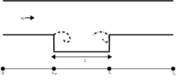
Geometry of a thermoacoustic system with a backward facing step. Total length of the chamber is denoted by
 $l_{a}$
. Vortex formation occurs at
 $x_{sep}$
and vortex breakdown occurs at
 $x_{c}$
. This figure is not drawn to scale.

In this study, a kick is a sharp rise in pressure due to vortex breakdown. The amplitude of the pressure rise is given by the circulation strength of the vortex that impinged. The time period between kicks is the time interval between two consecutive vortex breakdowns. For a classical delta-kicked harmonic oscillator, both the time period between the kicks and the strength of the kick remain constant. The same is not true for our system because both are dependent on the pressure and velocity fluctuations in the system, which are in turn governed by nonlinear equations. Therefore, it is not straightforward to derive a Poincaré map for this system. We overcome this obstacle by assuming small fluctuations, low strength of the kicks and that the time intervals between the kicks are constant. The Poincaré map derived under this assumption is useful in studying the stability of the system.
The outline of this manuscript is as follows. In § 2, we recall the theory describing the vortex shedding and chamber acoustics. In § 3, we derive the Poincaré map relating the velocity and pressure fluctuations between successive kicks. In § 4 we present the results of the linear stability analysis for our thermoacoustic system. In § 5 we compare the results obtained using the Poincaré map with the experimental observations available in the literature. Finally, in § 6 we present the concluding remarks of our work.
2 Theory
In this section we present the theory and the equations governing the thermoacoustic system. In order to fully describe the system, we need models for vortex shedding and chamber acoustics. The outline of this section is as follows. First, we present the governing equations for vortex shedding in unsteady flows and use them in the thermoacoustic model. Next, we use Galerkin decomposition to reduce the obtained partial differential equations into a set of ordinary differential equations. After that, we present the procedure to compute the fluctuations at any given point in the system. Finally, we discuss the approximations used in obtaining the Poincaré map.
2.1 Model for vortex shedding
The vortex shedding process is modelled using the method described by Matveev & Culick (Reference Matveev and Culick2003). The thermoacoustic system studied here is a combustor with a backward facing step as shown in figure 1. The total length of the acoustic chamber is denoted by
 $l_{a}$
. A backward facing step of height
 $d$
is located at
 $x_{sep}$
. This is the point where vortex separation occurs. The separated vortex impinges and breaks down at the point denoted by
 $x_{c}$
. The length of the cavity is represented by
 $l_{c}$
.
At certain flow velocities the shear layer at the lip (
 $x_{sep}$
) becomes unstable, and vortex formation occurs. When the vortices are shed, they convect in the cavity and impinge on the wall of the combustor which is present downstream. The equations governing the vortex formation, convection and breakdown are nonlinear. In the following subsections, we recall the model for vortex shedding process in unsteady flows developed by Matveev & Culick (Reference Matveev and Culick2003).
2.1.1 Vortex shedding frequency
In case of a steady state flow, the non-dimensional vortex shedding frequency (
 $f_{s0}$
) is given by
 $$\begin{eqnarray}\displaystyle f_{s0}=St\frac{M}{d}, & & \displaystyle\end{eqnarray}$$
where
 $M$
is the Mach number,
 $St$
is the Strouhal number, assumed to be constant in certain ranges of the Reynolds number (Lienhard Reference Lienhard1966), and the characteristic size
 $d$
is the height of the backward facing step non-dimensionalised using
 $l_{a}$
. The non-dimensional time period
 ${\it\tau}_{s0}$
between two consecutive vortex separations, for a steady state flow, is given by
 $$\begin{eqnarray}{\it\tau}_{s0}=\frac{1}{St}\frac{d}{M}.\end{eqnarray}$$
2.1.2 Circulation of a vortex
Fluctuations in pressure (
 $p^{\prime }$
) and velocity (
 $u^{\prime }$
) affect the vortex shedding process. Matveev & Culick (Reference Matveev and Culick2003) formulated a reduced-order model to describe vortex shedding in unsteady flows. The non-dimensional rate of circulation production is given by
 $$\begin{eqnarray}\displaystyle & \displaystyle \frac{\text{d}{\it\Gamma}_{m}}{\text{d}t}=M\frac{1}{2}[1+u^{\prime }(x_{sep},t)]^{2}, & \displaystyle\end{eqnarray}$$
where
 ${\it\Gamma}_{m}$
denotes the circulation of the
 $m\text{th}$
vortex generated. A vortex separation occurs when its circulation
 ${\it\Gamma}_{m}$
reaches a critical value,
 ${\it\Gamma}_{sep}$
, defined by the momentary flow velocity. The non-dimensional critical circulation (
 ${\it\Gamma}_{sep}$
) is given by
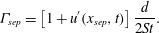 $$\begin{eqnarray}\displaystyle & \displaystyle {\it\Gamma}_{sep}=\left[1+u^{\prime }(x_{sep},t)\right]\frac{d}{2St}. & \displaystyle\end{eqnarray}$$
2.1.3 Vortex convection velocity
The velocity of a shed vortex depends on the total flow velocity at the instantaneous position of the vortex. Since a vortex moves along the boundary between the primary flow and the recirculation zone, its steady velocity component is lower than that of the primary flow. Dotson, Koshigoe & Pace (Reference Dotson, Koshigoe and Pace1997) approximated the velocity of the shed vortex using the relation
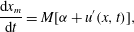 $$\begin{eqnarray}\displaystyle & \displaystyle \frac{\text{d}x_{m}}{\text{d}t}=M[{\it\alpha}+u^{\prime }(x,t)], & \displaystyle\end{eqnarray}$$
where
 $x_{m}$
is the instantaneous location of the
 $m\text{th}$
vortex and
 ${\it\alpha}$
is a coefficient usually chosen to be in the range 0.4–0.6.
2.2 The thermoacoustic model
Assuming uniform density
 ${\it\rho}_{0}$
, for a low Mach number approximation, the non-dimensional momentum and energy equations, which govern the acoustic field of this system, are written as follows:
 $$\begin{eqnarray}\displaystyle & \displaystyle \frac{\partial u^{\prime }}{\partial t}+\frac{\partial p^{\prime }}{\partial x}=0, & \displaystyle\end{eqnarray}$$
 $$\begin{eqnarray}\displaystyle & \displaystyle \frac{\partial p^{\prime }}{\partial t}+\frac{\partial u^{\prime }}{\partial x}+{\it\zeta}p^{\prime }=\frac{({\it\gamma}-1)}{{\it\gamma}}\frac{{\it\beta}}{M}\mathop{\sum }_{m}{\it\Gamma}_{m}{\it\delta}(t-t_{m}){\it\delta}(x-x_{c}). & \displaystyle\end{eqnarray}$$
The heat addition rate in (2.7) is modelled by assuming the energy release is proportional to the vortex circulation
 ${\it\Gamma}_{m}$
and that the vortex burning is localized both in space (
 $x_{c}$
) where the vortex impinges and time (
 $t_{m}$
) when the
 $m\text{th}$
vortex impinges (Matveev & Culick Reference Matveev and Culick2003). The symbol
 ${\it\gamma}$
denotes the heat capacity ratio,
 ${\it\beta}$
is the unsteady heat release coefficient and
 ${\it\zeta}$
is the acoustic damping term artificially added to the (2.7). The ends of the acoustic chamber are assumed to be open.
The following scales are chosen for non-dimensionalising the equations governing the vortex shedding process and the acoustic flow field:
 $$\begin{eqnarray}\begin{array}{@{}l@{}}\displaystyle M=\frac{u_{0}}{c_{0}};\quad u^{\prime }=\frac{\tilde{u} ^{\prime }}{u_{0}};\quad p^{\prime }=\frac{\tilde{p}^{\prime }}{{\it\gamma}Mp_{0}};\quad t=\frac{c_{0}}{l_{a}}\tilde{t};\quad x=\frac{\tilde{x}}{l_{a}}.\end{array}\end{eqnarray}$$
In (2.8), the steady state quantities are velocity (
 $u_{0}$
), pressure (
 $p_{0}$
) and the speed of sound (
 $c_{0}$
). The other dimensional quantities are denoted with a tilde above them, such as the velocity fluctuation (
 $\tilde{u} ^{\prime }$
), pressure fluctuation (
 $\tilde{p}^{\prime }$
) and time (
 $\tilde{t}$
). In case of non-dimensional quantities, the tildes are dropped.
2.3 Decomposition using Galerkin modes
The non-dimensional partial differential equations (2.6) and (2.7) are reduced to a set of ordinary differential equations (ODEs) by expanding the acoustic variables in terms of basis functions using the Galerkin technique. The mode shapes chosen for decomposing
 $u^{\prime }$
and
 $p^{\prime }$
are
 $\cos (k_{n}x)$
and
 $\sin (k_{n}x)$
so that the open–open boundary conditions of the acoustic system are satisfied.
 $$\begin{eqnarray}u^{\prime }=\mathop{\sum }_{n=1}^{N}\cos (k_{n}x)U_{n}(t),\quad p^{\prime }=\mathop{\sum }_{n=1}^{N}\sin (k_{n}x)P_{n}(t)\end{eqnarray}$$
are Galerkin decomposition for the fluctuations in velocity and pressure. In (2.9a,b
)
 $U_{n}$
,
 $P_{n}$
are the amplitude of the
 $n\text{th}$
Galerkin modes and
 $k_{n}=n{\rm\pi}$
is the non-dimensional wavenumber of the
 $n\text{th}$
mode. The duct modes in the absence of a heat source have non-dimensional frequencies
 $f=0.5n$
and time periods
 $T=2/n$
for
 $n=\{1,2,\ldots N\}$
, where
 $N$
is the number of Galerkin modes. The non-dimensional angular frequency of the
 $n\text{th}$
duct mode is
 ${\it\omega}_{n}=n{\rm\pi}$
.
Substituting (2.9a,b ) into the partial differential equations (2.6) and (2.7) gives the following set of ODEs for the momentum and energy equation:
 $$\begin{eqnarray}\displaystyle & \displaystyle \dot{U}_{n}+k_{n}P_{n}=0, & \displaystyle\end{eqnarray}$$
 $$\begin{eqnarray}\displaystyle & \displaystyle {\dot{P}}_{n}+2{\it\zeta}_{n}P_{n}-k_{n}U_{n}=2\frac{({\it\gamma}-1)}{{\it\gamma}}\frac{{\it\beta}}{M}\sin (k_{n}x_{c})\mathop{\sum }_{m}{\it\Gamma}_{m}{\it\delta}(t-t_{m}). & \displaystyle\end{eqnarray}$$
In (2.11), following Matveev & Culick (Reference Matveev and Culick2003), the damping term
 ${\it\zeta}$
is rewritten as a frequency-dependent damping term
 ${\it\zeta}_{n}$
given by
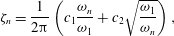 $$\begin{eqnarray}{\it\zeta}_{n}=\frac{1}{2{\rm\pi}}\left(c_{1}\frac{{\it\omega}_{n}}{{\it\omega}_{1}}+c_{2}\sqrt{\frac{{\it\omega}_{1}}{{\it\omega}_{n}}}\right),\end{eqnarray}$$
where
 $c_{1}$
and
 $c_{2}$
are the damping coefficients which are responsible for the end loses and loses due to boundary layers respectively (Sterling & Zukoski Reference Sterling and Zukoski1991). Substituting
 ${\it\omega}_{n}=n{\rm\pi}$
in (2.12) gives
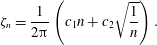 $$\begin{eqnarray}\displaystyle & \displaystyle {\it\zeta}_{n}=\frac{1}{2{\rm\pi}}\left(c_{1}n+c_{2}\sqrt{\frac{1}{n}}\right). & \displaystyle\end{eqnarray}$$
We rewrite the system of coupled first-order differential equations (2.10) and (2.11) as a second-order differential equation in
 $U_{n}$
.
 $$\begin{eqnarray}\displaystyle & \displaystyle \ddot{U} _{n}+2{\it\zeta}_{n}{\it\omega}_{n}\dot{U}_{n}+k_{n}^{2}U_{n}=-2k_{n}\frac{({\it\gamma}-1)}{{\it\gamma}}\frac{{\it\beta}}{M}\sin (k_{n}x_{c})\mathop{\sum }_{m}{\it\Gamma}_{m}{\it\delta}(t-t_{m}) & \displaystyle\end{eqnarray}$$
represents the dynamics of the thermoacoustic system presented. The dynamics is similar to that of a kicked oscillator, which behaves as a damped oscillator when the kicks are absent. The jump in
 $U_{n}$
and
 $P_{n}$
are obtained by integrating equations (2.10) and (2.11) in the time interval
 $t_{m}^{-}$
–
 $t_{m}^{+}$
, which corresponds to the time instants just before and after the breakdown of the
 $m\text{th}$
vortex.
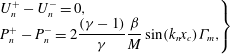 $$\begin{eqnarray}\displaystyle \left.\begin{array}{@{}l@{}}\displaystyle U_{n}^{+}-U_{n}^{-}=0,\\ \displaystyle P_{n}^{+}-P_{n}^{-}=2\frac{({\it\gamma}-1)}{{\it\gamma}}\frac{{\it\beta}}{M}\sin (k_{n}x_{c}){\it\Gamma}_{m},\end{array}\right\} & & \displaystyle\end{eqnarray}$$
gives the jump in velocity and pressure when a vortex impinges on the combustor wall. The strength of the
 $m\text{th}$
kick for a fixed geometric configuration is determined by
 ${\it\beta}{\it\Gamma}_{m}/M\sim {\it\beta}/f_{s0}$
. For a given
 ${\it\beta}/f_{s0}$
if damping is high, the fluctuations are quickly damped. We elaborate on this in § 4.2.
2.4 Procedure to compute the fluctuations
 $u^{\prime }$
and
$p^{\prime }$


First, we set the geometric parameters
 $\{x_{sep},x_{c},d\}$
and the flow parameters
 $\{M,c_{1},c_{2},{\it\alpha},{\it\beta},St\}$
. Next, we choose the size of the time step
 $\text{d}t$
, the number of time steps and the number of Galerkin modes
 $N$
. Then, we solve for
 $U_{n}$
and
 $\dot{U}_{n}$
from (2.14) using a fourth-order Runge–Kutta method. The above computation is performed in the absence of kicking
 $(t\neq t_{m})$
so the right-hand side of (2.14) is set to zero. After that, we compute the circulation at
 $x_{sep}$
using (2.3) and the critical circulation using (2.4). If
 ${\it\Gamma}_{m}\geqslant {\it\Gamma}_{sep}$
, the
 $m\text{th}$
vortex is shed and the circulation is reset to zero. The circulation of the
 $(m+1)\text{th}$
vortex is computed in the next time step. All separated vortices in the cavity are convected using (2.5). If a vortex impinges at
 $x_{c}$
, the jump conditions given by (2.15) are applied. Thus, the non-periodic Dirac delta function on the right-hand side of (2.14) is handled. The same is repeated for desired number of time steps. Finally, the fluctuations at any location can be computed using (2.9a,b
).
2.5 Linear approximations used for the model
The dynamics of the system described by (2.14) and (2.15) is nonlinear in general because of the coupling between the fluctuations in the flow and the dynamics of vortex formation. In this paper, linear stability analysis is performed to study the dynamics of this system. In the absence of acoustic fluctuations, vortex shedding and breakdown occur with a time period
 ${\it\tau}_{s0}$
. We begin the analysis in the limit of small fluctuations and low values of
 ${\it\beta}/f_{s0}$
. Even in this limit, the time interval between successive kicks (
 ${\it\tau}$
) is not constant,
 ${\it\tau}={\it\tau}_{s0}+{\it\epsilon}{\it\tau}_{s0}$
, with
 ${\it\epsilon}\ll 1$
. This correction in the time period has an
 ${\it\epsilon}$
first-order effect in the calculation of
 ${\it\Gamma}_{m}$
using (2.3). This in turn leads to a correction of same order in the energy (2.11) and hence on the dynamics of the system. However, within the current framework, in order to obtain an analytical solution, the time periods of kicks and shedding are assumed to be constant and equal to
 ${\it\tau}_{s0}$
. This assumption leads to an additional approximation, apart from that due to the assumption of small fluctuations and low
 ${\it\beta}/f_{s0}$
. Hence the results should be used as a first estimate for the nonlinear simulations. In this study, the above discussed assumptions are collectively termed the linear approximations. One can then obtain an analytical solution for the flow variables associated with vortex dynamics.
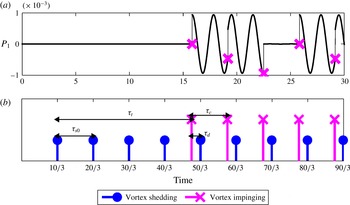
Figure 2(a) shows the time evolution of the Galerkin mode
 $P_{1}$
for
 $M=0.03$
from nonlinear simulations. The system behaves like a damped harmonic oscillator except at the time of the kicks. At the time instant when a kick occurs there is a jump in the amplitude of
 $P_{1}$
(cf. (2.15)).
(a) Time evolution of the amplitude of Galerkin mode
 $P_{1}$
. The time instants just before the kick are marked with the symbol ‘
 $\times$
’.
 $(b)$
Time instants when vortex separation and breakdown occurs are shown. Also, the various relevant time periods are marked. The system parameters used for the simulation are as follows:
 $M=0.03,c_{1}=0.315\times 10^{-3},c_{2}=0.015\times 10^{-3},{\it\beta}=10^{-3},{\it\alpha}=0.4,x_{sep}=0.3,x_{c}=0.45$
,
 $St=0.1$
and
 $d=0.01$
.

For a system with no initial excitations, the time period between two consecutive vortex shedding events
 ${\it\tau}_{s0}$
is given by (2.2). For
 $M=0.03$
,
 $St=0.1$
and
 $d=0.01$
, this time period
 ${\it\tau}_{s0}=10/3$
. In figure 2(b), we can see that the first vortex separates exactly at time
 ${\it\tau}_{s0}$
after the flow has started. The subsequent sheddings are also after the same time interval before the first shed vortex impinges at
 $x_{c}$
. Under our linear approximations, since the time periods of the vortex shedding and impinging events are the same and equal to
 ${\it\tau}_{s0}$
, the convection velocity of the vortex is constant. Dropping the term
 $Mu^{\prime }(x,t)$
from (2.5) gives us
 $$\begin{eqnarray}{\dot{x}}_{m}=M{\it\alpha}.\end{eqnarray}$$
Then, the time
 ${\it\tau}_{t}$
taken by a separated vortex to traverse the distance
 $l_{c}$
, from
 $x_{sep}$
to
 $x_{c}$
is given by
 $$\begin{eqnarray}{\it\tau}_{t}=\frac{l_{c}}{M{\it\alpha}}.\end{eqnarray}$$
The first vortex impinges on the combustor wall at time
 ${\it\tau}_{s0}+{\it\tau}_{t}$
. In figure 2(a) it can be seen that until the first impingement, the amplitude of the Galerkin mode
 $P_{1}$
is zero because no energy release has occurred and there has been no initial excitation. As soon as the first vortex impinges we can see a jump in
 $P_{1}$
. From there on, the system behaves like a damped harmonic oscillator at all time instants except when a kick occurs (vortex impingement and breakdown occurs).
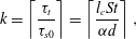
In figure 2(b) it can be seen that four vortices are shed at time intervals of
 ${\it\tau}_{s0}$
before the first vortex impinged on the wall. In general, the number of vortices shed,
 $k$
, before the first vortex impinges on the wall is given by
 $$\begin{eqnarray}k=\left\lceil \frac{{\it\tau}_{t}}{{\it\tau}_{s0}}\right\rceil =\left\lceil \frac{l_{c}St}{{\it\alpha}d}\right\rceil ,\end{eqnarray}$$
where
 $\left\lceil x\right\rceil$
denotes the largest integer greater than or equal to
 $x$
.
The circulation and time of separation of the
 $(k+1)\text{th}$
vortex will be affected by energy released due to the impingement of the first vortex and the time interval between the first impingement and the
 $(k+1)\text{th}$
shedding. By induction, the circulation strength of the
 $(k+m)\text{th}$
vortex depends on the energy released by the impingement of the
 $m\text{th}$
vortex and the time interval between the impingement of the
 $m\text{th}$
vortex and shedding of the
 $(k+m)\text{th}$
vortex. This time interval is denoted by
 ${\it\tau}_{d}$
and is given by the expression
 $$\begin{eqnarray}{\it\tau}_{d}=k{\it\tau}_{s0}-{\it\tau}_{t}.\end{eqnarray}$$
All time intervals
 ${\it\tau}_{s0},{\it\tau}_{c},{\it\tau}_{t}$
and
 ${\it\tau}_{d}$
are marked in figure 2(b) for reference. Further, to emphasize, in our linear approximation,
 ${\it\tau}_{c},{\it\tau}_{t}$
and
 ${\it\tau}_{d}$
are all constants with
 ${\it\tau}_{c}={\it\tau}_{s0}$
. In the next section, we derive the Poincaré map for the Galerkin modes. This map can be used to perform linear stability analysis on the thermoacoustic system modelled.
3 Derivation of the Poincaré map
In this section, we derive the Poincaré map under the assumptions discussed in § 2.5. Next, we rewrite the equations in a more convenient matrix notation. Finally, we present the procedure to calculate the fixed points and their stability. The dynamics of each of the
 $N$
Galerkin modes behave like independent kicked oscillators, except at the instants of the kicks. The Poincaré map gives a relation among the Galerkin modes between two consecutive kicks. Hence the map is called a kick-to-kick Poincaré map. The time period between the kicks is taken to be
 ${\it\tau}_{c}(={\it\tau}_{s0})$
, which is the time period between two consecutive vortex breakdowns.
The evolution of the Galerkin modes given by (2.14) reduces to the following second-order differential equation
 $$\begin{eqnarray}\displaystyle & \displaystyle \ddot{U} _{n}+2{\it\zeta}_{n}k_{n}\dot{U}_{n}+k_{n}^{2}U_{n}=0, & \displaystyle\end{eqnarray}$$
in the absence of kick or in the time between the kicks.
3.1 Solution to damped simple harmonic oscillator
Equation (3.1) represents a damped harmonic oscillator. This equation has three solutions, namely under damped (
 ${\it\zeta}_{n}<1$
), over damped (
 ${\it\zeta}_{n}>1$
) and critically damped (
 ${\it\zeta}_{n}=1$
). For the time being, we focus only on the under damped case, for which the solutions for
 $U_{n}$
and
 $P_{n}$
are given as follows:
 $$\begin{eqnarray}\displaystyle U_{n}(t) & = & \displaystyle \text{e}^{-{\it\zeta}_{n}k_{n}t}\left[A\cos \left(\sqrt{1-{\it\zeta}_{n}^{2}}k_{n}t\right)+B\sin \left(\sqrt{1-{\it\zeta}_{n}^{2}}k_{n}t\right)\right],\end{eqnarray}$$
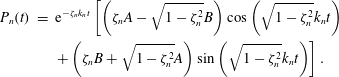 $$\begin{eqnarray}\displaystyle P_{n}(t) & = & \displaystyle \text{e}^{-{\it\zeta}_{n}k_{n}t}\left[\left({\it\zeta}_{n}A-\sqrt{1-{\it\zeta}_{n}^{2}}B\right)\cos \left(\sqrt{1-{\it\zeta}_{n}^{2}}k_{n}t\right)\right.\nonumber\\ \displaystyle & & \displaystyle \left.+\left({\it\zeta}_{n}B+\sqrt{1-{\it\zeta}_{n}^{2}}A\right)\sin \left(\sqrt{1-{\it\zeta}_{n}^{2}}k_{n}t\right)\right].\end{eqnarray}$$
In (3.2) and (3.3), setting
 $t=0$
gives the value of the constants
 $A$
and
 $B$
as follows:
 $$\begin{eqnarray}A=U_{n}(0),\quad B=\frac{{\it\zeta}_{n}U_{n}(0)-P_{n}(0)}{\sqrt{1-{\it\zeta}_{n}^{2}}}.\end{eqnarray}$$
Substituting the values of the constants
 $A$
and
 $B$
into (3.2) and (3.3) and introducing a new variable
 ${\it\Omega}_{n}=k_{n}\sqrt{1-{\it\zeta}_{n}^{2}}$
gives
 $$\begin{eqnarray}\displaystyle U_{n}(t) & = & \displaystyle \text{e}^{-{\it\zeta}_{n}k_{n}t}\left[U_{n}(0)\cos ({\it\Omega}_{n}t)+\frac{{\it\zeta}_{n}U_{n}(0)-P_{n}(0)}{\sqrt{1-{\it\zeta}_{n}^{2}}}\sin ({\it\Omega}_{n}t)\right],\end{eqnarray}$$
 $$\begin{eqnarray}\displaystyle P_{n}(t) & = & \displaystyle \text{e}^{-{\it\zeta}_{n}k_{n}t}\left[P_{n}(0)\cos ({\it\Omega}_{n}t)+\frac{U_{n}(0)-{\it\zeta}_{n}P_{n}(0)}{\sqrt{1-{\it\zeta}_{n}^{2}}}\sin ({\it\Omega}_{n}t)\right].\end{eqnarray}$$
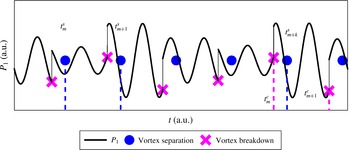
Representative time evolution of the Galerkin mode
 $P_{1}$
shown in some arbitrary time interval. The amplitude of the jump due to vortex breakdown at
 $t_{m}^{c}$
depends on the circulation strength of the vortex that separated at time
 $t_{m}^{s}$
.

3.2 The jump conditions
Figure 3 shows a representative time evolution of
 $P_{1}$
computed using the nonlinear simulations. Vortex separation occurs at time instants
 $\{t_{1}^{s},t_{2}^{s},\ldots ,t_{m}^{s},t_{m+1}^{s},\ldots \}$
. The vortex that separated at the instant
 $t_{m}^{s}$
impinges on the wall at time instant
 $t_{m}^{c}$
. The difference
 $t_{m}^{c}-t_{m}^{s}$
is given by
 ${\it\tau}_{t}$
(cf. (2.17)), the time taken by the vortex to traverse the cavity. The jump in
 $P_{1}$
at time
 $t_{m}^{c}$
depends on the circulation of the vortex that separated at time
 $t_{m}^{s}$
. Hence the jump conditions given by (2.15) become
 $$\begin{eqnarray}\left.\begin{array}{@{}c@{}}\displaystyle U_{n}(t_{m+}^{c})=U_{n}(t_{m-}^{c}),\\ \displaystyle P_{n}(t_{m+}^{c})=P_{n}(t_{m-}^{c})+\frac{({\it\gamma}-1)}{{\it\gamma}}\frac{{\it\beta}}{M}\sin (k_{n}x_{c})\left[1+\mathop{\sum }_{n=1}^{N}\cos (k_{n}x_{c})U_{n}(t_{m}^{s})\right]\frac{d}{St},\end{array}\right\}\end{eqnarray}$$
after the
 $m\text{th}$
vortex impinges on the wall. The amplitudes of
 $P_{n}(t_{m+}^{c})$
depend on the fluctuations in velocity
 $U_{n}(t_{m}^{s})$
. The kick strength is given by
 ${\it\beta}d/(MSt)={\it\beta}/f_{s0}$
. Therefore, we use the parameter
 ${\it\beta}/f_{s0}$
as one of the free parameters of the system.
3.3 The map equation
The amplitude of the Galerkin modes before the
 $(m+1)\text{th}$
kick is obtained by replacing the initial conditions
 $U_{n}(0),P_{n}(0)$
in (3.5) and (3.6) with the jump conditions
 $U_{n}(t_{m+}^{c}),P_{n}(t_{m+}^{c})$
given by (3.7). The map thus derived is as follows:
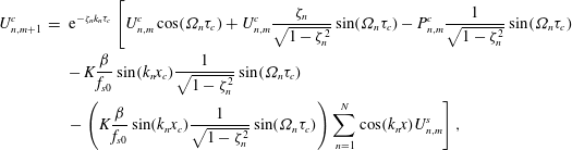 $$\begin{eqnarray}\displaystyle U_{n,m+1}^{c} & = & \displaystyle \text{e}^{-{\it\zeta}_{n}k_{n}{\it\tau}_{c}}\left[U_{n,m}^{c}\cos ({\it\Omega}_{n}{\it\tau}_{c})+U_{n,m}^{c}\frac{{\it\zeta}_{n}}{\sqrt{1-{\it\zeta}_{n}^{2}}}\sin ({\it\Omega}_{n}{\it\tau}_{c})-P_{n,m}^{c}\frac{1}{\sqrt{1-{\it\zeta}_{n}^{2}}}\sin ({\it\Omega}_{n}{\it\tau}_{c})\right.\nonumber\\ \displaystyle & & \displaystyle -\,K\frac{{\it\beta}}{f_{s0}}\sin (k_{n}x_{c})\frac{1}{\sqrt{1-{\it\zeta}_{n}^{2}}}\sin ({\it\Omega}_{n}{\it\tau}_{c})\nonumber\\ \displaystyle & & \displaystyle \left.-\left(K\frac{{\it\beta}}{f_{s0}}\sin (k_{n}x_{c})\frac{1}{\sqrt{1-{\it\zeta}_{n}^{2}}}\sin ({\it\Omega}_{n}{\it\tau}_{c})\right)\mathop{\sum }_{n=1}^{N}\cos (k_{n}x)U_{n,m}^{s}\right],\end{eqnarray}$$
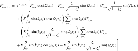 $$\begin{eqnarray}\displaystyle P_{n,m+1}^{c} & = & \displaystyle \text{e}^{-{\it\zeta}_{n}k_{n}{\it\tau}_{c}}\left[P_{n,m}^{c}\cos ({\it\Omega}_{n}{\it\tau}_{c})-P_{n,m}^{c}\frac{{\it\zeta}_{n}}{\sqrt{1-{\it\zeta}_{n}^{2}}}\sin ({\it\Omega}_{n}{\it\tau}_{c})+U_{n,m}^{c}\frac{1}{\sqrt{1-{\it\zeta}_{n}^{2}}}\sin ({\it\Omega}_{n}{\it\tau}_{c})\right.\nonumber\\ \displaystyle & & \displaystyle +\left(K\frac{{\it\beta}}{f_{s0}}\sin (k_{n}x_{c})\cos ({\it\Omega}_{n}{\it\tau}_{c})\right)\mathop{\sum }_{n=1}^{N}\cos (k_{n}x)U_{n,m}^{s}\nonumber\\ \displaystyle & & \displaystyle -\left(K\frac{{\it\beta}}{f_{s0}}\sin (k_{n}x_{c})\frac{{\it\zeta}_{n}}{\sqrt{1-{\it\zeta}_{n}^{2}}}\sin ({\it\Omega}_{n}{\it\tau}_{c})\right)\mathop{\sum }_{n=1}^{N}\cos (k_{n}x)U_{n,m}^{s}\nonumber\\ \displaystyle & & \displaystyle \left.+\,K\frac{{\it\beta}}{f_{s0}}\sin (k_{n}x_{c})\cos ({\it\Omega}_{n}{\it\tau}_{c})-K\frac{{\it\beta}}{f_{s0}}\sin (k_{n}x_{c})\frac{{\it\zeta}_{n}}{\sqrt{1-{\it\zeta}_{n}^{2}}}\sin ({\it\Omega}_{n}{\it\tau}_{c})\right],\end{eqnarray}$$
where
 $K=({\it\gamma}-1)/{\it\gamma}$
.
In (3.8) and (3.9), the amplitude of the modes just before the kick are denoted by
 $U_{n,m+1}^{c}$
and
 $P_{n,m+1}^{c}$
, where
 $n$
denotes the Galerkin mode number and
 $m$
the kick number. The map equations are coupled because
 $U_{n,m+1}^{c}=f(U_{n,m}^{c},P_{n,m}^{c},U_{n,m}^{s})$
, where the mode
 $U_{n,m}^{s}$
quantifies the strength of the
 $m\text{th}$
kick. We recall from § 3.2 that the strength of the first
 $k$
kicks are constant until the impingement of the first vortex. The strength of the
 $(k+1)\text{th}$
kick depends on the fluctuations created by the impingement of the first kick. A map for the strength of the kicks is obtained by replacing
 ${\it\tau}_{c}$
in (3.8) with
 ${\it\tau}_{d}$
, the time interval between the
 $m\text{th}$
kick and the
 $(m+k)\text{th}$
shedding. Before writing the map explicitly for
 $U_{n,m}^{s}$
, we introduce new variables to make equations (3.8) and (3.9) compact.
Let
 $$\begin{eqnarray}\displaystyle A_{n}({\it\tau}) & = & \displaystyle \text{e}^{-{\it\zeta}_{n}k_{n}{\it\tau}}\left[\cos ({\it\Omega}_{n}{\it\tau})+\frac{{\it\zeta}_{n}}{\sqrt{1-{\it\zeta}_{n}^{2}}}\sin ({\it\Omega}_{n}{\it\tau})\right],\end{eqnarray}$$
 $$\begin{eqnarray}\displaystyle B_{n}({\it\tau}) & = & \displaystyle \text{e}^{-{\it\zeta}_{n}k_{n}{\it\tau}}\frac{1}{\sqrt{1-{\it\zeta}_{n}^{2}}}\sin ({\it\Omega}_{n}{\it\tau}),\end{eqnarray}$$
 $$\begin{eqnarray}\displaystyle C_{n}({\it\tau}) & = & \displaystyle \text{e}^{-{\it\zeta}_{n}k_{n}{\it\tau}}K\frac{{\it\beta}}{f_{s0}}\sin (k_{n}x_{c})\frac{1}{\sqrt{1-{\it\zeta}_{n}^{2}}}\sin ({\it\Omega}_{n}{\it\tau}),\end{eqnarray}$$
 $$\begin{eqnarray}\displaystyle D_{n}({\it\tau}) & = & \displaystyle \text{e}^{-{\it\zeta}_{n}k_{n}{\it\tau}}\left[\cos ({\it\Omega}_{n}{\it\tau})-\frac{{\it\zeta}_{n}}{\sqrt{1-{\it\zeta}_{n}^{2}}}\sin ({\it\Omega}_{n}{\it\tau})\right],\end{eqnarray}$$
 $$\begin{eqnarray}\displaystyle F_{n}({\it\tau}) & = & \displaystyle \text{e}^{-{\it\zeta}_{n}k_{n}{\it\tau}}K\frac{{\it\beta}}{f_{s0}}\sin (k_{n}x_{c})\cos ({\it\Omega}_{n}{\it\tau}).\end{eqnarray}$$
Using (3.10)–(3.14) the Poincaré map given by (3.8) and (3.9) is now written as
 $$\begin{eqnarray}\displaystyle U_{n,m+1}^{c} & = & \displaystyle A_{n}^{c}U_{n,m}^{c}-B_{n}^{c}P_{n,m}^{c}-C_{n}^{c}\mathop{\sum }_{n=1}^{N}\cos (k_{n}x)U_{n,m}^{s}-C_{n}^{c},\end{eqnarray}$$
 $$\begin{eqnarray}\displaystyle P_{n,m+1}^{c} & = & \displaystyle B_{n}^{c}U_{n,m}^{c}+D_{n}^{c}P_{n,m}^{c}+(F_{n}^{c}-{\it\zeta}_{n}C_{n}^{c})\mathop{\sum }_{n=1}^{N}\cos (k_{n}x)U_{n,m}^{s}+F_{n}^{c}-{\it\zeta}_{n}C_{n}^{c},\end{eqnarray}$$
where
 $A_{n}^{c}=A_{n}({\it\tau}_{c}),B_{n}^{c}=B_{n}({\it\tau}_{c}),\ldots$
and similarly for other terms. To compute the strength of each kick we write another map equation as follows:
 $$\begin{eqnarray}U_{n,m+k}^{s}=A_{n}^{s}U_{n,m}^{c}-B_{n}^{s}P_{n,m}^{c}-C_{n}^{s}\mathop{\sum }_{n=1}^{N}\cos (k_{n}x)U_{n,m}^{s}-C_{n}^{s},\end{eqnarray}$$
where
 $A_{n}^{s}=A_{n}({\it\tau}_{d}),B_{n}^{s}=B_{n}({\it\tau}_{d}),\ldots$
and similarly for other terms. Note that the map for shedding relates the amplitudes of the modes at the
 $(m+k)\text{th}$
instant with the amplitude of the modes at the
 $m\text{th}$
instant.
Equations (3.15), (3.16) and (3.17) represent the kick-to-kick Poincaré map of the thermoacoustic system. For the purpose of analytical study, these equations are recast in a matrix form. The matrix representation of (3.15) is as follows:
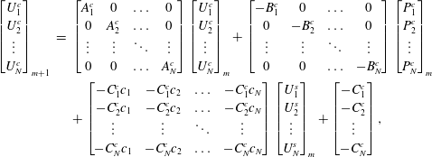 $$\begin{eqnarray}\displaystyle \left[\begin{array}{@{}c@{}}U_{1}^{c}\\ U_{2}^{c}\\ \vdots \\ U_{N}^{c}\\ \end{array}\right]_{m+1} & = & \displaystyle \left[\begin{array}{@{}cccc@{}}A_{1}^{c} & 0 & \ldots & 0\\ 0 & A_{2}^{c} & \ldots & 0\\ \vdots & \vdots & \ddots & \vdots \\ 0 & 0 & \ldots & A_{N}^{c}\\ \end{array}\right]\left[\begin{array}{@{}c@{}}U_{1}^{c}\\ U_{2}^{c}\\ \vdots \\ U_{N}^{c}\\ \end{array}\right]_{m}+\left[\begin{array}{@{}cccc@{}}-B_{1}^{c} & 0 & \ldots & 0\\ 0 & -B_{2}^{c} & \ldots & 0\\ \vdots & \vdots & \ddots & \vdots \\ 0 & 0 & \ldots & -B_{N}^{c}\\ \end{array}\right]\left[\begin{array}{@{}c@{}}P_{1}^{c}\\ P_{2}^{c}\\ \vdots \\ P_{N}^{c}\\ \end{array}\right]_{m}\nonumber\\ \displaystyle & & \displaystyle +\left[\begin{array}{@{}cccc@{}}-C_{1}^{c}c_{1} & -C_{1}^{c}c_{2} & \ldots & -C_{1}^{c}c_{N}\\ -C_{2}^{c}c_{1} & -C_{2}^{c}c_{2} & \ldots & -C_{2}^{c}c_{N}\\ \vdots & \vdots & \ddots & \vdots \\ -C_{N}^{c}c_{1} & -C_{N}^{c}c_{2} & \ldots & -C_{N}^{c}c_{N}\\ \end{array}\right]\left[\begin{array}{@{}c@{}}U_{1}^{s}\\ U_{2}^{s}\\ \vdots \\ U_{N}^{s}\\ \end{array}\right]_{m}+\left[\begin{array}{@{}c@{}}-C_{1}^{c}\\ -C_{2}^{c}\\ \vdots \\ -C_{N}^{c}\\ \end{array}\right],\end{eqnarray}$$
where
 $c_{n}=\cos (k_{n}x_{sep})$
. Similarly, (3.16) and (3.17) can also be recast in matrix form.
Let
 $\{\boldsymbol{{\it\eta}},{\bf\psi},{\bf\sigma}\}$
denote the column matrices
 $\{U_{n}^{c},P_{n}^{c},U_{n}^{s}\}$
, then the map given by (3.18) becomes
 $$\begin{eqnarray}\boldsymbol{{\it\eta}}_{m+1}=\unicode[STIX]{x1D648}_{A}^{c}\boldsymbol{{\it\eta}}_{m}-\unicode[STIX]{x1D648}_{B}^{c}{\bf\psi}_{m}+\unicode[STIX]{x1D648}_{C}^{c}{\bf\sigma}_{m}+\unicode[STIX]{x1D64D}_{1}^{c},\end{eqnarray}$$
where
 $\unicode[STIX]{x1D648}_{A}^{c},\unicode[STIX]{x1D648}_{B}^{c},\unicode[STIX]{x1D648}_{C}^{c}$
(cf. appendix A) are the propagator matrices in (3.18) and
 $\unicode[STIX]{x1D64D}_{1}^{c}$
(cf. appendix B) is the constant column matrix. Similarly, the maps given by (3.16) and (3.17) become
 $$\begin{eqnarray}\displaystyle {\bf\psi}_{m+1} & = & \displaystyle \unicode[STIX]{x1D648}_{B}^{c}\boldsymbol{{\it\eta}}_{m}+\unicode[STIX]{x1D648}_{D}^{c}{\bf\psi}_{m}+\unicode[STIX]{x1D648}_{F}^{c}{\bf\sigma}_{m}+\unicode[STIX]{x1D64D}_{2}^{c},\end{eqnarray}$$
 $$\begin{eqnarray}\displaystyle {\bf\sigma}_{m+k} & = & \displaystyle \unicode[STIX]{x1D648}_{A}^{s}\boldsymbol{{\it\eta}}_{m}-\unicode[STIX]{x1D648}_{B}^{s}{\bf\psi}_{m}+\unicode[STIX]{x1D648}_{C}^{s}{\bf\sigma}_{m}+\unicode[STIX]{x1D64D}_{1}^{s},\end{eqnarray}$$
where the matrices
 $\unicode[STIX]{x1D648}_{D}^{c}$
,
 $\unicode[STIX]{x1D648}_{F}^{c}$
,
 $\unicode[STIX]{x1D648}_{A}^{s},\unicode[STIX]{x1D648}_{B}^{s},\unicode[STIX]{x1D648}_{C}^{s}$
are given in appendix A and
 $\unicode[STIX]{x1D64D}_{2}^{c}$
,
 $\unicode[STIX]{x1D64D}_{1}^{s}$
are given in appendix B.
3.4 Procedure to calculate the fixed points
A fixed point of a map represents an equilibrium solution of (3.19)–(3.21). To calculate the fixed points we set
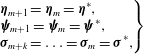 $$\begin{eqnarray}\left.\begin{array}{@{}l@{}}\displaystyle \boldsymbol{{\it\eta}}_{m+1}=\boldsymbol{{\it\eta}}_{m}=\boldsymbol{{\it\eta}}^{\ast },\\ \displaystyle {\bf\psi}_{m+1}={\bf\psi}_{m}={\bf\psi}^{\ast },\\ \displaystyle {\bf\sigma}_{m+k}=\ldots ={\bf\sigma}_{m}={\bf\sigma}^{\ast },\end{array}\!\!\!\right\}\end{eqnarray}$$
in (3.19)–(3.21). Then, the fixed points
 $\{\boldsymbol{{\it\eta}}^{\ast },{\bf\psi}^{\ast },{\bf\sigma}^{\ast }\}$
are the solution to the following system of linear equations:
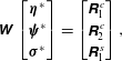 $$\begin{eqnarray}\displaystyle \unicode[STIX]{x1D652}\left[\begin{array}{@{}c@{}}\boldsymbol{{\it\eta}}^{\ast }\\ {\bf\psi}^{\ast }\\ {\bf\sigma}^{\ast }\\ \end{array}\right]=\left[\begin{array}{@{}c@{}}\unicode[STIX]{x1D64D}_{1}^{c}\\ \unicode[STIX]{x1D64D}_{2}^{c}\\ \unicode[STIX]{x1D64D}_{1}^{s}\\ \end{array}\right], & & \displaystyle\end{eqnarray}$$
where
 $\unicode[STIX]{x1D652}$
is a
 $3\times N$
matrix given in appendix C.
 $N$
denotes the total number of Galerkin modes. When
 $\unicode[STIX]{x1D652}$
is singular, the fixed points have no solution or infinite solutions. We observe in § 4.3 that matrix
 $\unicode[STIX]{x1D652}$
is not singular for the range of parameters explored in this study. Our next task here is to quantify whether the fixed points
 $\{\boldsymbol{{\it\eta}}^{\ast },{\bf\psi}^{\ast },{\bf\sigma}^{\ast }\}$
computed using (3.23) are linearly stable or unstable.
3.5 Procedure to calculate the stability of fixed points
For a stable fixed point disturbances around it decay with time and conversely for an unstable fixed point, they grow over time. For a linear map of the form
 ${\it\chi}_{m+1}=\unicode[STIX]{x1D648}{\it\chi}_{m}$
, the fixed points are stable if all the eigenvalues of
 $\unicode[STIX]{x1D648}$
lie inside a unit circle and becomes unstable when the maximum eigenvalue crosses the unit circle. The matrix
 $\unicode[STIX]{x1D648}$
for the thermoacoustic system is obtained as follows.
The Poincaré map (3.21) is not a first-order difference equation because it relates the
 ${\bf\sigma}$
at the
 $(m+k)\text{th}$
instant with the
 ${\bf\sigma}$
at the
 $m\text{th}$
instant. This map is rewritten as
 $$\begin{eqnarray}\displaystyle & \displaystyle {\bf\sigma}_{m+1}=\unicode[STIX]{x1D648}_{A}^{s}\boldsymbol{{\it\eta}}_{m-k+1}-\unicode[STIX]{x1D648}_{B}^{s}{\bf\psi}_{m-k+1}+\unicode[STIX]{x1D648}_{C}^{s}{\bf\sigma}_{m-k+1}+\unicode[STIX]{x1D64D}_{1}^{s}, & \displaystyle\end{eqnarray}$$
so that the relation is between the values at the
 $(m+1)\text{th}$
instant and the
 $(m-k+1)\text{th}$
instant. Then, using change of variables the
 $k\text{th}$
-order difference equation (3.24) is converted into a set of first-order difference equations. This conversion is desirable for the purpose of stability analysis. The following change of variables are used.
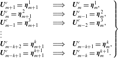 $$\begin{eqnarray}\left.\begin{array}{@{}lcl@{}}\displaystyle \boldsymbol{U}_{m+1}^{c}=\boldsymbol{{\it\eta}}_{m+1}^{1}\quad & \;\Longrightarrow \;\quad & \boldsymbol{U}_{m}^{c}=\boldsymbol{{\it\eta}}_{m}^{1},\\ \displaystyle \boldsymbol{U}_{m}^{c}=\boldsymbol{{\it\eta}}_{m+1}^{2}\quad & \;\Longrightarrow \;\quad & \boldsymbol{U}_{m-1}^{c}=\boldsymbol{{\it\eta}}_{m}^{2},\\ \displaystyle \boldsymbol{U}_{m-1}^{c}=\boldsymbol{{\it\eta}}_{m+1}^{3}\quad & \;\Longrightarrow \;\quad & \boldsymbol{U}_{m-2}^{c}=\boldsymbol{{\it\eta}}_{m}^{3},\\ \vdots \quad & \quad & \\ \displaystyle \boldsymbol{U}_{m-k+2}^{c}=\boldsymbol{{\it\eta}}_{m+1}^{k}\quad & \;\Longrightarrow \;\quad & \boldsymbol{U}_{m-k+1}^{c}=\boldsymbol{{\it\eta}}_{m}^{k},\\ \displaystyle \boldsymbol{U}_{m-k+1}^{c}=\boldsymbol{{\it\eta}}_{m+1}^{k+1}\quad & \;\Longrightarrow \;\quad & \boldsymbol{U}_{m-k}^{c}=\boldsymbol{{\it\eta}}_{m}^{k+1}.\end{array}\right\}\end{eqnarray}$$
Similar changes of variables are performed for
 $\boldsymbol{P}^{c}$
and
 $\boldsymbol{U}^{s}$
. Substituting (3.25) and their counterparts for
 $\boldsymbol{P}^{c}$
and
 $\boldsymbol{U}^{s}$
in (3.19)–(3.21) gives
 $$\begin{eqnarray}\displaystyle \boldsymbol{{\it\eta}}_{m+1}^{1} & = & \displaystyle \unicode[STIX]{x1D648}_{A}^{c}\boldsymbol{{\it\eta}}_{m}^{1}-\unicode[STIX]{x1D648}_{B}^{c}{\bf\psi}_{m}^{1}+\unicode[STIX]{x1D648}_{C}^{c}{\bf\sigma}_{m}^{1}+\unicode[STIX]{x1D64D}_{1}^{c},\end{eqnarray}$$
 $$\begin{eqnarray}\displaystyle {\bf\psi}_{m+1}^{1} & = & \displaystyle \unicode[STIX]{x1D648}_{B}^{c}\boldsymbol{{\it\eta}}_{m}^{1}+\unicode[STIX]{x1D648}_{D}^{c}{\bf\psi}_{m}^{1}+\unicode[STIX]{x1D648}_{F}^{c}{\bf\sigma}_{m}^{1}+\unicode[STIX]{x1D64D}_{2}^{c},\end{eqnarray}$$
 $$\begin{eqnarray}\displaystyle {\bf\sigma}_{m+1}^{1} & = & \displaystyle \unicode[STIX]{x1D648}_{A}^{s}\boldsymbol{{\it\eta}}_{m}^{k}-\unicode[STIX]{x1D648}_{B}^{s}{\bf\psi}_{m}^{k}+\unicode[STIX]{x1D648}_{C}^{s}{\bf\sigma}_{m}^{k}+\unicode[STIX]{x1D64D}_{1}^{s}.\end{eqnarray}$$
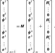
When all the linear equations are cast in a matrix form we obtain the following relation for the linear map of the system:
 $$\begin{eqnarray}\displaystyle \left[\begin{array}{@{}c@{}}\boldsymbol{{\it\eta}}^{1}\\ \vdots \\ \boldsymbol{{\it\eta}}^{k}\\ {\bf\psi}^{1}\\ \vdots \\ {\bf\psi}^{k}\\ {\bf\sigma}^{1}\\ \vdots \\ {\bf\sigma}^{k}\\ \end{array}\right]_{m+1}=\unicode[STIX]{x1D648}\left[\begin{array}{@{}c@{}}\boldsymbol{{\it\eta}}^{1}\\ \vdots \\ \boldsymbol{{\it\eta}}^{k}\\ {\bf\psi}^{1}\\ \vdots \\ {\bf\psi}^{k}\\ {\bf\sigma}^{1}\\ \vdots \\ {\bf\sigma}^{k}\\ \end{array}\right]_{m}+\left[\begin{array}{@{}c@{}}\unicode[STIX]{x1D64D}_{1}^{c}\\ \vdots \\ \boldsymbol{ 0}\\ \unicode[STIX]{x1D64D}_{2}^{c}\\ \vdots \\ \boldsymbol{ 0}\\ \unicode[STIX]{x1D64D}_{1}^{s}\\ \vdots \\ \boldsymbol{ 0}\\ \end{array}\right], & & \displaystyle\end{eqnarray}$$
where
 $\unicode[STIX]{x1D648}$
is a
 $3\times N\times k$
matrix given in appendix C and
 $\mathbf{0}$
is a zero vector of length
 $N$
. The eigenvalues of
 $\unicode[STIX]{x1D648}$
form the set
 $\{{\it\lambda}_{1},{\it\lambda}_{2},\ldots ,{\it\lambda}_{3\times n\times k}\}$
. The system has a stable fixed point if the maximum of the absolute value of the eigenvalues is less than one. Mathematically the fixed point is stable if
 $$\begin{eqnarray}|{\it\lambda}_{max}|=\sup \{|{\it\lambda}_{1}|,|{\it\lambda}_{2}|,\ldots ,|{\it\lambda}_{3\times n\times k}|\}<1.\end{eqnarray}$$
Otherwise the fixed point is unstable.
4 Results
We study the evolution of the thermoacoustic system for different flow parameters using the Poincaré map. The outline of the section is as follows. First, we present the parameters for the configuration of the system. Next, we compare the nonlinear simulations with the Poincaré map. Then, we compute the fixed points for the chosen system configurations. After that, we compute the stability of the fixed points. Finally, we discuss the implications of the results obtained.
4.1 System parameters chosen for the study
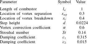
The free parameters in the system are broadly classified into two categories – the geometric and the flow parameters. In this study we fix the geometry of the combustor
 $\{x_{sep},x_{c},d,l_{a}\}$
and vary only the flow parameters. The parameters that define the operating conditions are the Mach number
 $M$
, damping coefficients
 $\{c_{1},c_{2}\}$
, the vortex convection coefficient
 ${\it\alpha}$
and the unsteady heat release coefficient
 ${\it\beta}$
. We fix
 ${\it\alpha}$
to be 0.6 (cf. Dotson et al.
Reference Dotson, Koshigoe and Pace1997) for all the case studies. The values of the damping coefficients
 $\{c_{1},c_{2}\}$
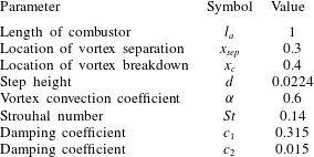
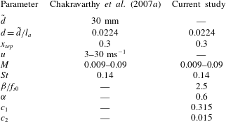
are same as those given in Sterling & Zukoski (Reference Sterling and Zukoski1991). The chosen geometric and the flow parameters are shown in table 1. The geometry of the configuration is similar to the one investigated by Chakravarthy et al. (Reference Chakravarthy, Shreenivasan, Boehm, Dreizler and Janicka2007a
), as we later compare our results with their experiments in § 5.1. The Mach number investigated is
 $M\leqslant 0.1$
, because we work with low Mach number approximation.
For the nonlinear simulation, the size of the time step is set to be
 $\text{d}t=10^{-4}$
and the number of Galerkin modes
 $N=32$
. We found that if the size of the time step is decreased from
 $10^{-4}$
to
 $10^{-5}$
, the computed
 $u^{\prime },p^{\prime }$
change by
 ${<}1\,\%$
. Hence, we choose a time step of
 $10^{-4}$
. The number of modes chosen in this study is higher than the number chosen by Matveev & Culick (Reference Matveev and Culick2003), Tulsyan et al. (Reference Tulsyan, Balasubramanian and Sujith2009) and Subramanian et al. (Reference Subramanian, Mariappan, Sujith and Wahi2010) for similar problems. One mode approximation is used to derive some analytical results using the Poincaré map.
System parameters chosen for the study.
The
 $u^{\prime }$
fluctuations at
 $x_{sep}$
for
 $M=0.029$
: (a,b)
 ${\it\beta}=0.048$
or
 ${\it\beta}/f_{s0}=0.27$
, (c,d)
 ${\it\beta}=0.48$
or
 ${\it\beta}/f_{s0}=2.7$
and (e,f)
 ${\it\beta}=0.51$
or
 ${\it\beta}/f_{s0}=2.83$
. For all the chosen values of
 ${\it\beta}/f_{s0}$
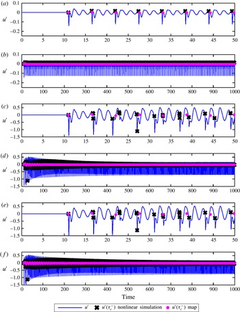
, the fixed points computed by the nonlinear simulations and the map agree with each other for long time cycles but the difference in the converged value increases. Even though
 $u^{\prime }$
peaks when vortex breakdown occurs, the peaks are quickly damped and the root mean squares of the
 $u^{\prime }$
fluctuations are 0.024, 0.15 and 0.18 respectively.

4.2 Comparison between the nonlinear simulation and the map
The linear approximation used in this paper is valid for low values of
 ${\it\beta}/f_{s0}$
, where the nonlinear simulations and the linear map agree with each other. In this section, we determine the threshold for
 ${\it\beta}/f_{s0}$
, above which the linear theory is not investigated. Figure 4(a–f) shows the
 $u^{\prime }$
fluctuations at
 $x_{sep}$
for three different values of
 ${\it\beta}=\{0.048,0.48,0.51\}$
. The peaks in
 $u^{\prime }$
appear only at the instants when vortex breakdown occurs. These peaks are quickly damped and the root mean square value of the fluctuations remain small for all of the cases. For each value of
 ${\it\beta}$
, we show the
 $u^{\prime }$
fluctuations for both short time scales (50 units cf. figure 4
a,c,e) and long time scales (1000 units cf. figure 4
b,d,f). As the strength of the kicks depend on the quantity
 ${\it\beta}/f_{s0}$
, we use the same to distinguish the cases instead of
 ${\it\beta}$
. For the chosen values of
 ${\it\beta}$
the value of
 ${\it\beta}/f_{s0}=\{0.27,2.7,2.8\}$
, where
 $f_{s0}=0.18$
.
In figure 4(a) we observe that, for
 ${\it\beta}/f_{s0}=0.27$
, the fluctuations vary between 0.04 and
 $-0.13$
. The root mean square of the
 $u^{\prime }$
fluctuations is 0.0245. Figure 4(b) shows that both the non-linear simulations and the map converge towards the same fixed point. The difference in the fixed point between the nonlinear simulation (after 1000 cycles) and the map is
 $5\times 10^{-4}$
. Similar results are observed for
 ${\it\beta}/f_{s0}=2.7$
(cf. figure 4
c,d) and
 ${\it\beta}/f_{s0}=2.8$
(cf. figure 4
e,f). The difference in the fixed points for these cases are
 $2\times 10^{-3}$
and
 $2\times 10^{-2}$
respectively. For
 ${\it\beta}/f_{s0}>2.85$
, the linear map does not agree with the nonlinear simulations. Therefore, we place the threshold for
 ${\it\beta}/f_{s0}$
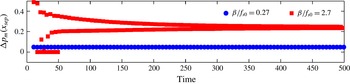
at 2.7. Furthermore, figure 5 shows the pressure rise (
 ${\rm\Delta}p_{m}(x_{sep})=p(x_{sep},t_{m}^{+})-p(x_{sep},t_{m}^{-})$
) at
 $x_{sep}$
for values of
 ${\it\beta}/f_{s0}=0.27,2.7$
. Since damping is high, the fluctuations at
 $x_{sep}$
are small for both values of
 ${\it\beta}/f_{s0}$
. For the rest of the study we only investigate conditions for which
 ${\it\beta}/f_{s0}<2.7$
.
For
 $M=0.029$
, pressure rise (
 ${\rm\Delta}p_{m}$
) at
 $x_{sep}$
just after the impingement of the
 $m\text{th}$
vortex obtained from the nonlinear simulations for various values of
 ${\it\beta}/f_{s0}$
.

4.3 Fixed points for the chosen system
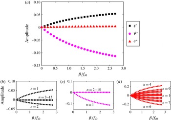
Fixed points for
 $M=0.05$
: (a)
 $\{\boldsymbol{{\it\eta}}^{\ast },{\bf\psi}^{\ast },{\bf\sigma}^{\ast }\}$
for the first mode. (b)
 $\boldsymbol{{\it\eta}}^{\ast }$
, (c)
 ${\bf\psi}^{\ast }$
, (d)
 ${\bf\sigma}^{\ast }$
for the first 15 modes. In (b) and (c) only the first mode is dominant, the remaining modes have a fixed point very close to zero. In (d) the first nine modes have a non-zero fixed point.

The fixed points of the system are computed using the procedure described in § 3.4. From (3.23), we observe that the fixed points depend on
 $\unicode[STIX]{x1D652}$
. When
 $|\unicode[STIX]{x1D652}|=0$
, fixed points have no solution or infinite solutions. We first examine the cases for which the matrix
 $\unicode[STIX]{x1D652}$
is singular. We compute
 $|\unicode[STIX]{x1D652}|$
using the symbolic-maths tool (Matlab) using a one mode approximation. The determinant of
 $\unicode[STIX]{x1D652}$
is a function of
 $M$
and
 ${\it\beta}$
. We set the Mach number as a free parameter and equate the expression for
 $|\unicode[STIX]{x1D652}|$
to zero. This gives us the value
 ${\it\beta}_{0}$
for which the matrix
 $\unicode[STIX]{x1D652}$
is singular. The expression for
 ${\it\beta}_{0}$
is given in appendix E. It is observed that the value of
 ${\it\beta}_{0}$
for which the matrix becomes singular is always greater than the threshold
 ${\it\beta}$
(or
 ${\it\beta}/f_{s0}$
) explored in this study. Hence, for the conditions investigated, the fixed points from the map are unique.
For
 $M=0.05$
, the heat release coefficient
 ${\it\beta}/f_{s0}$
is varied from
 $0\leqslant {\it\beta}/f_{s0}\leqslant 2.7$
and the fixed points are computed. Figure 6(a) shows the fixed points of the first mode for
 $\{\boldsymbol{{\it\eta}}^{\ast },{\bf\psi}^{\ast },{\bf\sigma}^{\ast }\}$
. Figure 6(b–d) shows the fixed points for the first 15 modes of
 $\{\boldsymbol{{\it\eta}}^{\ast },{\bf\psi}^{\ast },{\bf\sigma}^{\ast }\}$
. From these figures we observe that the first mode is dominant for
 $\boldsymbol{{\it\eta}}^{\ast },{\bf\psi}^{\ast }$
. The remaining modes reach fixed points close to zero for the same. While in figure 6(d), many modes reach non-zero fixed points.
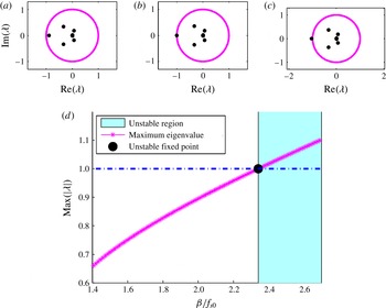
The eigenvalues of
 $\unicode[STIX]{x1D648}$
for
 $M=0.05$
: (a)
 ${\it\beta}/f_{s0}=2$
, (b)
 ${\it\beta}/f_{s0}=2.341$
and (c)
 ${\it\beta}/f_{s0}=2.5$
. (d) Stability of the fixed point as a function of
 ${\it\beta}$
. The value
 ${\it\beta}_{c}/f_{s0}=2.341$
corresponds to an unstable fixed point and the system is unstable for all
 ${\it\beta}>{\it\beta}_{c}$
.

4.4 Stability of the fixed points for the chosen system
The stability of the fixed point is computed using the procedure described in § 3.5. For
 $M=0.05$
,
 ${\it\beta}/f_{s0}$
is varied from
 $1.4\leqslant {\it\beta}/f_{s0}\leqslant 2.7$
and the eigenvalues of matrix
 $\unicode[STIX]{x1D648}$
(cf. appendix D) are computed for the configuration given in table 1. Figure 7(a–c) shows the movement of eigenvalues of matrix
 $\unicode[STIX]{x1D648}$
from the region inside a unit circle to the region outside the unit circle for increasing values of
 ${\it\beta}/f_{s0}$
. The value of
 ${\it\beta}/f_{s0}$
at which the system becomes unstable is denoted by
 $\left.{\it\beta}/f_{s0}\right|_{c}$
. Figure 7(d) shows the amplitude of the maximum eigenvalue of
 $\unicode[STIX]{x1D648}$
as
 ${\it\beta}/f_{s0}$
is varied in the range
 $1.4\leqslant {\it\beta}/f_{s0}\leqslant 2.7$
. When
 ${\it\beta}/f_{s0}=2$
, the absolute value of the eigenvalues are less than unity. In this region the system is linearly stable. When
 ${\it\beta}/f_{s0}=2.5$
, the amplitude of the maximum eigenvalue is greater than one. Therefore, the system is linearly unstable. The transition occurs at
 $\left.{\it\beta}/f_{s0}\right|_{c}=2.341$
, for which the maximum eigenvalue lies on the unit circle.
4.5 Eigenvectors
The eigenvector corresponding to the maximum eigenvalue of
 $\unicode[STIX]{x1D648}$
(cf. appendix D) is computed for the configuration given in table 1. The other free parameters are set as
 $M=0.05$
and
 ${\it\beta}/f_{s0}=\{0.27,2.7\}$
. The length of this eigenvector is
 $3\times N\times k$
. Where
 $N$
is the number of Galerkin modes set as 15 and
 $k(=1)$
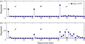
is the number of vortices shed before the first vortex impinged (cf. (2.18)). Figure 8(a,b) shows the different portions
 $\{\boldsymbol{{\it\eta}}_{N}^{k},{\bf\psi}_{N}^{k},{\bf\sigma}_{N}^{k}\}$
of the computed eigenvector. For
 ${\it\beta}/f_{s0}=0.27$
(cf. figure 8
a) we observe the first mode to be dominant
 $\{\boldsymbol{{\it\eta}}_{1}^{1},{\bf\psi}_{1}^{1},{\bf\sigma}_{1}^{1}\}$
. However, for
 ${\it\beta}/f_{s0}=2.7$
(cf. figure 8
b), when the system is linearly unstable, many modes are dominant for
 ${\bf\sigma}^{1}$
.
Eigenvector corresponding to the maximum eigenvalue of
 $\unicode[STIX]{x1D648}$
for
 $M=0.05$
and the configuration given in table 1. (a)
 ${\it\beta}/f_{s0}=0.27$
,
 $(b)$
 ${\it\beta}/f_{s0}=2.7$
Each component
 $\{\boldsymbol{{\it\eta}}_{1},{\bf\psi}_{1},{\bf\sigma}_{1}\}$
has fifteen modes in total.

5 Discussion
5.1 Outline on experimental investigations
We compare the results of our study with the experimental investigations of Chakravarthy et al. (Reference Chakravarthy, Shreenivasan, Boehm, Dreizler and Janicka2007a
,Reference Chakravarthy, Sivakumar and Shreenivasan
b
). In their study, thermoacoustic interactions were investigated for a range of air inlet velocities and fuel flow rates. The total length of the combustor configuration was
 $l_{a}=1.34$
m. For the purpose of comparison, all the lengths are non-dimensionalised using
 $l_{a}$
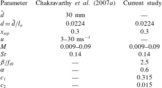
. The geometric and flow parameters obtained from the experiments are listed in table 2, along with the appropriate non-dimensional parameters used in this study. For the purpose of our analyses, all the parameters could not be obtained from the information given in the above experimental investigations. The damping coefficients
 $c_{1},c_{2}$
are chosen following the study by Sterling & Zukoski (Reference Sterling and Zukoski1991) for a similar configuration. The vortex convection coefficient
 ${\it\alpha}$
is chosen from the results given in Dotson et al. (Reference Dotson, Koshigoe and Pace1997). As there is no prescription available for the kick strength, we choose
 ${\it\beta}/f_{s0}=2.5$
.
An analogy between the parameters in the experiments of Chakravarthy et al. (Reference Chakravarthy, Shreenivasan, Boehm, Dreizler and Janicka2007a ) and the current study.
5.2 Method of comparison
Experimental investigations show the transition of the non-dimensional dominant frequency (Helmholtz number
 $He$
) between vortex shedding and acoustic mode when the air flow rate is varied. In this study, values of
 $He$
close to
 $0.5$
or
 $f_{s0}$
indicate that the first acoustic or vortex shedding mode is dominant, respectively. The steady state vortex shedding frequency
 $f_{s0}$
is a linear function of
 $M$
(cf. (2.1)). The present stability analysis can only predict the stability of the fixed point. The system is stable if all the eigenvalues of
 $\unicode[STIX]{x1D648}$
(cf. (D 1)) lie inside the unit circle and is unstable if the maximum eigenvalue lies outside the unit circle. Since the Poincaré map is constructed with the time interval of the steady state vortex shedding process, a stable system indicates that the vortex shedding mode is stable and hence dominant. On the other hand, when the system is unstable, this steady state vortex shedding mode is no longer dominant. Since the other mode of oscillation corresponds to the acoustic mode, this can possibly be the dominant mode.
5.3 Comparison with experiments of Chakravarthy et al. (Reference Chakravarthy, Shreenivasan, Boehm, Dreizler and Janicka2007a )
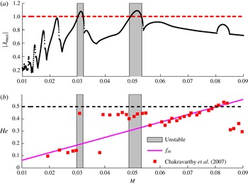
Figure 9(a) shows the absolute of the maximum eigenvalue (
 $|{\it\lambda}_{max}|$
) of
 $\unicode[STIX]{x1D648}$
as a function of Mach number for the experimental configuration investigated by Chakravarthy et al. (Reference Chakravarthy, Shreenivasan, Boehm, Dreizler and Janicka2007a
). From the present analysis, the system is unstable for
 $0.0299\leqslant M\leqslant 0.0321$
and
 $0.0488\leqslant M\leqslant 0.0532$
. Hence, the acoustic mode is expected to be dominant in these regimes, shown in grey. For other Mach numbers, vortex shedding mode is dominant. Figure 9(b) shows the variation of
 $He$
observed by Chakravarthy et al. (Reference Chakravarthy, Shreenivasan, Boehm, Dreizler and Janicka2007a
) as a function of Mach number. In their experimental investigation, Chakravarthy et al. (Reference Chakravarthy, Shreenivasan, Boehm, Dreizler and Janicka2007a
) observed that the dominant frequency transitions between the vortex shedding mode and acoustic mode when the Mach number is increased. They noted these transitions occur for
 $M=0.031,0.04,0.055$
and
 $0.085$
. The acoustic mode is dominant for
 $M=0.031$
and between
 $0.04{-}0.055$
.
Comparison between the map and experimental results given in Chakravarthy et al. (Reference Chakravarthy, Shreenivasan, Boehm, Dreizler and Janicka2007a ). (a) Amplitude of the maximum eigenvalue as a function of Mach number. (b) Helmholtz number observed by Chakravarthy et al. (Reference Chakravarthy, Shreenivasan, Boehm, Dreizler and Janicka2007a ) and the region of instability computed by linear stability analysis.

For
 $0.04\leqslant M\leqslant 0.055$
, the acoustic mode is observed to be dominant in the experiments. The present investigation predicts an unstable regime for
 $0.0488\leqslant M\leqslant 0.0532$
, which falls within the experimentally observed range. In another case, the experimental investigation reports that the acoustic mode is dominant for
 $M=0.031$
, while the analysis indicates that the unstable regime for
 $0.0299\leqslant M\leqslant 0.0321$
. The last transition at
 $M=0.085$
observed in the experiments is not captured by the analysis. Around
 $M=0.08$
, the numerical values of frequency associated with the vortex shedding and acoustic modes are the same. Hence the dominant mode cannot be identified. From the comparisons, it is observed that the present analysis under or over predicts the region where the acoustic mode is dominant. Two possible reasons for this discrepancy are discussed below.
The present analysis assumes small fluctuations, along with other approximations described in § 2.5, which is not true in the experiments. A number of parameters which determine the flow properties, namely the vortex convection coefficient
 ${\it\alpha}$
, the unsteady heat release coefficient
 ${\it\beta}$
and damping coefficients
 $c_{1},c_{2}$
could not be obtained from the information given in the experimental studies (Chakravarthy et al.
Reference Chakravarthy, Shreenivasan, Boehm, Dreizler and Janicka2007a
,Reference Chakravarthy, Sivakumar and Shreenivasan
b
). These values are chosen as given in the literature. To summarize, in the absence of nonlinear simulations and experimental results, this method of analysis can be used as a first estimate for obtaining the stability margin of the system.
6 Conclusion
We investigated a model combustor configuration where vortex formation and breakdown were the driving mechanisms for combustion instability. The interactions between the acoustic field and the unsteady heat release rate were modelled as a kicked oscillator. The energy released during vortex breakdown determines the strength of the kick. For small fluctuations, periodic and low values of kick, a Poincaré map is obtained analytically to study the thermoacoustic interactions. The stability of the system is determined from the absolute of the maximum eigenvalue associated with the obtained Poincaré map. This allows us to identify the dominant mode of oscillation. A stable system indicates that the vortex shedding mode is dominant. For the case when the system is unstable, the vortex shedding mode is no longer dominant and the acoustic mode is probably dominant. Previous experimental investigations report the transitions from vortex shedding to the acoustic mode of oscillation for variation in the Mach number. Similar transitions are predicted using the current analysis. These transitions are identified by the locations where the absolute of the maximum eigenvalue crosses unity. However, the analysis either over or under predicts the range where a given mode is dominant. This is attributed to the assumptions made in the analysis and non-availability of the numerical values of the flow parameters in the experiments. To conclude, this method of investigation can be used as a first estimate to determine the dominant modes of oscillations in the absence of nonlinear simulations and experiments.
Acknowledgements
The authors are grateful to the Indian Institute of Technology Kanpur for the financial support during the period of this research work, through post-doctoral fellowship and Initiation grant (IITK/AE/20130179). Further the authors thank the anonymous reviewers for their insightful comments which led to significant improvements in the manuscript.
Appendix A
Matrices used in the Poincaré map equation in §§ 3.3–3.5.
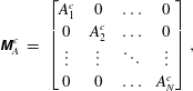 $$\begin{eqnarray}\displaystyle \unicode[STIX]{x1D648}_{A}^{c} & = & \displaystyle \left[\begin{array}{@{}cccc@{}}A_{1}^{c} & 0 & \ldots & 0\\ 0 & A_{2}^{c} & \ldots & 0\\ \vdots & \vdots & \ddots & \vdots \\ 0 & 0 & \ldots & A_{N}^{c}\\ \end{array}\right],\end{eqnarray}$$
where
 $A_{n}^{c}=A_{n}({\it\tau}_{c})$
. To obtain the matrix
 $\unicode[STIX]{x1D648}_{A}^{s}$
,
 $A_{n}^{c}$
is replaced with
 $A_{n}^{s}=A_{n}({\it\tau}_{d})$
in the above expression.
 $$\begin{eqnarray}\displaystyle \unicode[STIX]{x1D648}_{B}^{c} & = & \displaystyle \left[\begin{array}{@{}cccc@{}}B_{1}^{c} & 0 & \ldots & 0\\ 0 & B_{2}^{c} & \ldots & 0\\ \vdots & \vdots & \ddots & \vdots \\ 0 & 0 & \ldots & B_{N}^{c}\\ \end{array}\right],\end{eqnarray}$$
where
 $B_{n}^{c}=B_{n}({\it\tau}_{c})$
. To obtain the matrix
 $\unicode[STIX]{x1D648}_{B}^{s}$
,
 $B_{n}^{c}$
is replaced with
 $B_{n}^{s}=B_{n}({\it\tau}_{d})$
in the above expression.
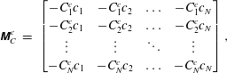 $$\begin{eqnarray}\displaystyle \unicode[STIX]{x1D648}_{C}^{c} & = & \displaystyle \left[\begin{array}{@{}cccc@{}}-C_{1}^{c}c_{1} & -C_{1}^{c}c_{2} & \ldots & -C_{1}^{c}c_{N}\\ -C_{2}^{c}c_{1} & -C_{2}^{c}c_{2} & \ldots & -C_{2}^{c}c_{N}\\ \vdots & \vdots & \ddots & \vdots \\ -C_{N}^{c}c_{1} & -C_{N}^{c}c_{2} & \ldots & -C_{N}^{c}c_{N}\\ \end{array}\right],\end{eqnarray}$$
where
 $C_{n}^{c}=C_{n}({\it\tau}_{c})$
. To obtain the matrix
 $\unicode[STIX]{x1D648}_{C}^{s}$
,
 $C_{n}^{c}$
is replaced with
 $C_{n}^{s}=C_{n}({\it\tau}_{d})$
in the above expression.
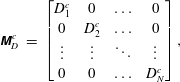 $$\begin{eqnarray}\displaystyle \unicode[STIX]{x1D648}_{D}^{c} & = & \displaystyle \left[\begin{array}{@{}cccc@{}}D_{1}^{c} & 0 & \ldots & 0\\ 0 & D_{2}^{c} & \ldots & 0\\ \vdots & \vdots & \ddots & \vdots \\ 0 & 0 & \ldots & D_{N}^{c}\\ \end{array}\right],\end{eqnarray}$$
where
 $D_{n}^{c}=D_{n}({\it\tau}_{c})$
.
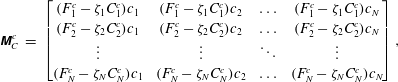 $$\begin{eqnarray}\displaystyle \unicode[STIX]{x1D648}_{C}^{c} & = & \displaystyle \left[\begin{array}{@{}cccc@{}}(F_{1}^{c}-{\it\zeta}_{1}C_{1}^{c})c_{1} & (F_{1}^{c}-{\it\zeta}_{1}C_{1}^{c})c_{2} & \ldots & (F_{1}^{c}-{\it\zeta}_{1}C_{1}^{c})c_{N}\\ (F_{2}^{c}-{\it\zeta}_{2}C_{2}^{c})c_{1} & (F_{2}^{c}-{\it\zeta}_{2}C_{2}^{c})c_{2} & \ldots & (F_{2}^{c}-{\it\zeta}_{2}C_{2}^{c})c_{N}\\ \vdots & \vdots & \ddots & \vdots \\ (F_{N}^{c}-{\it\zeta}_{N}C_{N}^{c})c_{1} & (F_{N}^{c}-{\it\zeta}_{N}C_{N}^{c})c_{2} & \ldots & (F_{N}^{c}-{\it\zeta}_{N}C_{N}^{c})c_{N}\\ \end{array}\right],\end{eqnarray}$$
where
 $F_{n}^{c}=F_{n}({\it\tau}_{c})$
.
Appendix B
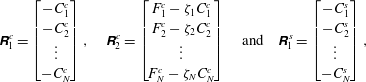 $$\begin{eqnarray}\displaystyle \unicode[STIX]{x1D64D}_{1}^{c}=\left[\begin{array}{@{}c@{}}-C_{1}^{c}\\ -C_{2}^{c}\\ \vdots \\ -C_{N}^{c}\\ \end{array}\right],\quad \unicode[STIX]{x1D64D}_{2}^{c}=\left[\begin{array}{@{}c@{}}F_{1}^{c}-{\it\zeta}_{1}C_{1}^{c}\\ F_{2}^{c}-{\it\zeta}_{2}C_{2}^{c}\\ \vdots \\ F_{N}^{c}-{\it\zeta}_{N}C_{N}^{c}\\ \end{array}\right]\quad \text{and}\quad \unicode[STIX]{x1D64D}_{1}^{s}=\left[\begin{array}{@{}c@{}}-C_{1}^{s}\\ -C_{2}^{s}\\ \vdots \\ -C_{N}^{s}\\ \end{array}\right], & & \displaystyle\end{eqnarray}$$
where
 $C_{n}^{c}=C_{n}({\it\tau}_{c})$
,
 $F_{n}^{c}=F_{n}({\it\tau}_{c})$
and
 $C_{n}^{s}=C_{n}({\it\tau}_{d})$
.
Appendix C
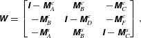 $$\begin{eqnarray}\displaystyle \unicode[STIX]{x1D652}=\left[\begin{array}{@{}ccc@{}}\unicode[STIX]{x1D644}-\unicode[STIX]{x1D648}_{A}^{c} & \unicode[STIX]{x1D648}_{B}^{c} & -\unicode[STIX]{x1D648}_{C}^{c}\\ -\unicode[STIX]{x1D648}_{B}^{c} & \unicode[STIX]{x1D644}-\unicode[STIX]{x1D648}_{D}^{c} & -\unicode[STIX]{x1D648}_{F}^{c}\\ -\unicode[STIX]{x1D648}_{A}^{s} & \unicode[STIX]{x1D648}_{B}^{s} & \unicode[STIX]{x1D644}-\unicode[STIX]{x1D648}_{C}^{s}\\ \end{array}\right], & & \displaystyle\end{eqnarray}$$
where
 $\unicode[STIX]{x1D644}$
is a
 $N\times N$
identity matrix and
 $N$
denotes the number of Galerkin modes.
Appendix D
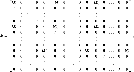 $$\begin{eqnarray}\displaystyle \unicode[STIX]{x1D648}=\left[\begin{array}{@{}ccccccccccccccc@{}}\unicode[STIX]{x1D648}_{A}^{c} & \mathbf{0} & \ldots & \mathbf{0} & \mathbf{0} & -\unicode[STIX]{x1D648}_{B}^{c} & \mathbf{0} & \ldots & \mathbf{0} & \mathbf{0} & \unicode[STIX]{x1D648}_{C}^{c} & \mathbf{0} & \ldots & \mathbf{0} & \mathbf{0}\\ \unicode[STIX]{x1D644} & \mathbf{0} & \ldots & \mathbf{0} & \mathbf{0} & \mathbf{0} & \mathbf{0} & \ldots & \mathbf{0} & \mathbf{0} & \mathbf{0} & \mathbf{0} & \ldots & \mathbf{0} & \mathbf{0}\\ \vdots & \vdots & \ddots & \vdots & \vdots & \vdots & \vdots & \ddots & \vdots & \vdots & \vdots & \vdots & \ddots & \vdots & \vdots \\ \mathbf{0} & \mathbf{0} & \ldots & \unicode[STIX]{x1D644} & \mathbf{0} & \mathbf{0} & \mathbf{0} & \ldots & \mathbf{0} & \mathbf{0} & \mathbf{0} & \mathbf{0} & \ldots & \mathbf{0} & \mathbf{0}\\ \unicode[STIX]{x1D648}_{B}^{c} & \mathbf{0} & \ldots & \mathbf{0} & \mathbf{0} & \unicode[STIX]{x1D648}_{D}^{c} & \mathbf{0} & \ldots & \mathbf{0} & \mathbf{0} & \unicode[STIX]{x1D648}_{F}^{c} & \mathbf{0} & \ldots & \mathbf{0} & \mathbf{0}\\ \mathbf{0} & \mathbf{0} & \ldots & \mathbf{0} & \mathbf{0} & \unicode[STIX]{x1D644} & \mathbf{0} & \ldots & \mathbf{0} & \mathbf{0} & \mathbf{0} & \mathbf{0} & \ldots & \mathbf{0} & \mathbf{0}\\ \vdots & \vdots & \ddots & \vdots & \vdots & \vdots & \vdots & \ddots & \vdots & \vdots & \vdots & \vdots & \ddots & \vdots & \vdots \\ \mathbf{0} & \mathbf{0} & \ldots & \mathbf{0} & \mathbf{0} & \mathbf{0} & \mathbf{0} & \ldots & \unicode[STIX]{x1D644} & \mathbf{0} & \mathbf{0} & \mathbf{0} & \ldots & \mathbf{0} & \mathbf{0}\\ \boldsymbol{ 0} & \mathbf{0} & \ldots & \mathbf{0} & \unicode[STIX]{x1D648}_{A}^{s} & \mathbf{0} & \mathbf{0} & \ldots & \mathbf{0} & \unicode[STIX]{x1D648}_{B}^{s} & \mathbf{0} & \mathbf{0} & \ldots & \mathbf{0} & \unicode[STIX]{x1D648}_{C}^{s}\\ \mathbf{0} & \mathbf{0} & \ldots & \mathbf{0} & \mathbf{0} & \mathbf{0} & \mathbf{0} & \ldots & \mathbf{0} & \mathbf{0} & \mathbf{0} & \unicode[STIX]{x1D644} & \ldots & \mathbf{0} & \mathbf{0}\\ \vdots & \vdots & \ddots & \vdots & \vdots & \vdots & \vdots & \ddots & \vdots & \vdots & \vdots & \vdots & \ddots & \vdots & \vdots \\ \mathbf{0} & \mathbf{0} & \ldots & \mathbf{0} & \mathbf{0} & \mathbf{0} & \mathbf{0} & \ldots & \mathbf{0} & \mathbf{0} & \mathbf{0} & \mathbf{0} & \ldots & \unicode[STIX]{x1D644} & \mathbf{0}\\ \end{array}\right], & & \displaystyle\end{eqnarray}$$
where
 $\mathbf{0}$
is a
 $N\times N$
zero matrix.
Appendix E
The value of the unsteady heat release rate for which the Poincaré map has multiple solutions for the fixed point.
 $$\begin{eqnarray}\displaystyle & \displaystyle {\it\beta}_{0}=\frac{1}{\cos (x_{sep}{\rm\pi})}\frac{1+(B_{1}^{\prime c})^{2}+A_{1}^{c}D_{1}^{c}-D_{1}^{c}}{Dr}, & \displaystyle\end{eqnarray}$$
where
 $$\begin{eqnarray}\displaystyle \displaystyle Dr & = & \displaystyle A_{1}^{c}D_{1}^{c}C_{1}^{\prime s}+A_{1}^{c}F_{1}^{\prime c}B_{1}^{\prime s}+(B_{1}^{\prime c})^{2}C_{1}^{\prime s}+B_{1}^{\prime c}C_{1}^{\prime c}A_{1}^{s}{\it\zeta}_{1}+C_{1}^{\prime c}A_{1}^{s}+C_{1}^{\prime s}\nonumber\\ \displaystyle & & \displaystyle \displaystyle -\,A_{1}^{c}C_{1}^{\prime s}-A_{1}^{c}C_{1}^{\prime c}B_{1}^{\prime s}{\it\zeta}_{1}-B_{1}^{\prime c}C_{1}^{\prime c}B_{1}^{\prime s}-B_{1}^{\prime c}F_{1}^{\prime c}A_{1}^{s}-C_{1}^{\prime c}D_{1}^{c}A_{1}^{s}-D_{1}^{c}C_{1}^{\prime s}-F_{1}^{\prime c}B_{1}^{\prime s},\qquad\end{eqnarray}$$
 $$\begin{eqnarray}B_{1}^{\prime c}=\frac{B_{1}^{c}}{{\it\beta}};\quad C_{1}^{\prime c}=\frac{C_{1}^{c}}{{\it\beta}};\quad F_{1}^{\prime c}=\frac{F_{1}^{c}}{{\it\beta}},\end{eqnarray}$$
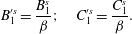 $$\begin{eqnarray}B_{1}^{\prime s}=\frac{B_{1}^{s}}{{\it\beta}};\quad C_{1}^{\prime s}=\frac{C_{1}^{s}}{{\it\beta}}.\end{eqnarray}$$