2. Experimental shape dynamics

Figure 1.

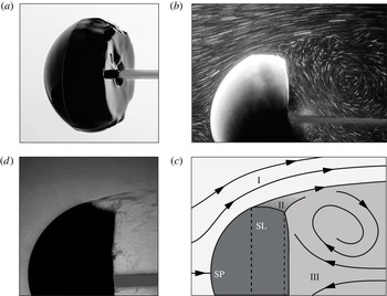
Dissolution of hard candy in flowing water. (a) The body starts as a sphere of diameter 6 cm, and the photograph shows the shape after 60 min of dissolution in a $30~\text{cm}~\text{s}^{-1}$ flow (left to right). (b) Streaklines obtained by seeding the flow with microparticles. (c) Schematic showing the outer flow (I), quiescent (II) and wake (III) regions. The flow meets the body at the stagnation point (SP) and detaches at the separation line (SL). (d) Shadowgraph imaging shows that highly concentrated solution is swept off the body at the SL.

We focus on bodies of simple initial shapes dissolving within unidirectional flows, with the hope of distilling principles that apply more generally. In particular, bodies of size $a\sim 1{-}10$  cm made of hard candy are placed within water flows of speed $U_{0}\sim 10{-}100~\text{cm}~\text{s}^{-1}$ . These scales yield a high Reynolds number $Re=aU_{0}/{\it\nu}\sim 10^{4}$ , where ${\it\nu}$ is the kinematic viscosity of water. Typical dissolving rates are $1~\text{cm h}^{-1}$ , indicating that the boundary motion is many orders slower than the flow speed. Specifically, amorphous solidified sugar – called hard candy in the USA or boiled sweets in the UK – is made by heating an 8:3:2 mixture by volume of table sugar (sucrose), light corn syrup and water to $302~\text{F}$ ( $150\,^{\circ }\text{C}$ ) and casting within moulds. Dissolution occurs within a water tunnel with test section $15~\text{cm}\times 15~\text{cm}\times 43~\text{cm}$ . Speed is continuously monitored by a laser Doppler velocimeter, and temperature is kept at $28\pm 1\,^{\circ }\text{C}$ .

Figure 2.

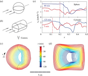
Shape evolution during dissolution. (a,b) Bodies of different initial shapes – a sphere and a cylinder with diameters of 6.0 and 6.9  cm, respectively – are presented with a flow of speed $30~\text{cm}~\text{s}^{-1}$ and photographed from below. (c,d) Interfaces displayed every $6$ min and colour-coded in time, with separation points indicated by the dotted line. (e) Comparison of the recession rate at locations along the body for the sphere (top) and cylinder (bottom) and at early (red) and late (blue) times. The arc length is $0$ at the front and $0.5$ at the back of the body, and separation is marked by dashed vertical lines.

Considering first a spherical initial geometry, we find that dissolution sculpts a unique shape that bears signatures of the flow. In figure 1(a), we show a photograph of the body removed after 60 min of dissolution in a flow of speed $30~\text{cm}~\text{s}^{-1}$ . The body is composed of a rounded front face, a facet that encircles the body and is bounded by two ridges, and a flattened back side. While the front has been polished smooth, both the facet and the back show surface irregularities, which are presumably associated with unsteady local flow. To visualize the flow field, we seed the water with microparticles (3M microbubbles), illuminate a plane with a laser sheet, and capture time-exposed photographs. The streakline photograph of figure 1(b) shows that the flow remains attached over the front surface of the body before separating at the leading ridge of the facet. As illustrated in the schematic of figure 1(c), the back sits within an unsteady wake, and the facet is associated with a quiescent region between separation and the wake. We also use shadowgraph imaging to visualize variations in the concentration of dissolved sugars (Garner & Hoffman Reference Garner and Hoffman1961). The image of figure 1(d) shows that the separation streamline carries a high solute concentration, suggesting that dissolution along the front face is confined to a thin layer that is then swept off the body.

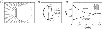
We capture the development of these surface features using time-lapsed photography and image analysis. The data of figure 2(c) show that the rounded face persists throughout the experiment, the back flattens relatively quickly, and the front and back surfaces approach one another, causing the intervening facet to shrink over time. The dynamics of the facet and the back appear to be closely related to the separated flow and wake region. The front surface, where flow is attached, experiences the highest dissolving rates and appears to be static in shape. However, careful inspection reveals that initial irregularities are smoothed over, suggesting that the rounded final shape is not simply a consequence of the initial shape. To test this idea, we consider a body that presents a flat wall to the flow, in particular a cylinder with one end facing upstream, as shown in figure 2(b), an arrangement that preserves axial symmetry. Interestingly, the front is rounded over time, as shown in figure 2(d). The emergence of this same final shape from different initial geometries suggests the existence of a stable attracting state for the fluid–structure dynamics.

The approach to this terminal state can be quantified by measuring how the dissolving rate varies both along the surface and at different times. In figure 2(e) we plot the normal velocity of the receding interface as a function of the arc length $s$ along the spherical (top) and cylindrical (bottom) bodies. The rate is shown at early (red) and later (blue) times, and the arc length at which flow separation occurs is indicated by a vertical dashed line. For both geometries, the velocity is variable along the front surface for early times, indicating a change of shape. For the sphere, these variations are slight and seem to be associated with manufacturing defects. For the cylinder, however, the rate is significantly lower near stagnation ( $s=0$ ) and higher at separation, which tends to round the initially flat face. In all cases, the rate along the front becomes more uniform at later times, thus tending to preserve the shape. Indeed, this self-similar recession is apparent from the even spacing between successive interfaces of figure 2(c,d) at later times.

3. Scaling laws

Figure 3.

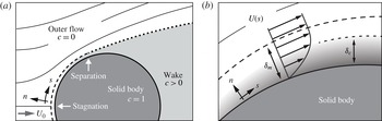
Schematics of the flow and concentration fields. (a) The steady outer flow consists of fresh water, while the attached flow near the body forms a boundary layer (dashed line) containing dissolved material. (b) Zoomed-in view of the momentum and concentration boundary layers (not to scale), the former defined by the flow velocity and the latter by the solute.

An understanding of these dynamics requires a model of how the concentration and flow fields affect dissolution. In the absence of flow, the solute simply diffuses and the boundary recedes at a rate given by Fick’s law, $v_{n}=-D\partial c/\partial n$ (Garner & Suckling Reference Garner and Suckling1958; Garner & Hoffman Reference Garner and Hoffman1961; Duda & Vrentas Reference Duda and Vrentas1971). Here, $D$ is the molecular diffusivity, $c$ is the concentration of dissolved material and $n$ is the surface normal. In the presence of flow, the washing away of solute tends to increase the concentration gradient and thus enhance the dissolution (Grijseels et al. Reference Grijseels, Crommelin and De Blaey1981). Similar ideas hold for forced thermal convection, where temperature is analogous to concentration and flow enhances the transfer of heat (Schlichting & Gersten Reference Schlichting and Gersten2000). For the mass transfer problem considered here, however, the flux of solute is associated with a change of shape and thus a change in the surrounding flow. As shown in figure 3(a,b), the attached flow along the front forms a momentum boundary layer of thickness ${\it\delta}_{m}$ in which the velocity rises from zero to a local outer flow value $U(s)$ (Childress Reference Childress2009). Similarly, the dissolved material is confined to a concentration boundary layer of thickness ${\it\delta}_{c}$ (Schlichting & Gersten Reference Schlichting and Gersten2000). The arrangement of these layers depends on the relative importance of viscosity ${\it\nu}$ and diffusivity $D$ , whose ratio is the Schmidt number $Sc={\it\nu}/D$ (or Prandtl number $Pr$ in thermal convection), and we estimate $Sc\sim 10^{3}$ in our experiments. Using an analogous relationship from thermal convection (Schlichting & Gersten Reference Schlichting and Gersten2000), we expect that ${\it\delta}_{c}/{\it\delta}_{m}\sim Sc^{-1/3}\sim 0.1$ . Thus, high $Sc$ indicates that viscosity dominates diffusion, and the solute is confined well within the flow boundary layer.

By considering how the boundary layer depends on the body size, we can incorporate the shape–flow interaction into scaling laws. For a flow of speed $U_{0}$ past a body of size $a$ , the Prandtl boundary-layer equations indicate ${\it\delta}_{m}\sim \sqrt{{\it\nu}a/U_{0}}$ (Schlichting & Gersten Reference Schlichting and Gersten2000). On retaining only the dependence on $a$ and $U_{0}$ and using ${\it\delta}_{c}\sim {\it\delta}_{m}$ from above, the interfacial velocity is then $v_{n}\sim 1/{\it\delta}_{c}\sim \sqrt{U_{0}/a}$ . 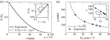The body volume $V\sim a^{3}$ satisfies $\text{d}V/\text{d}t\sim v_{n}a^{2}\sim \sqrt{U_{0}V}$ , and integration yields $V/V_{0}=(1-t/t_{f})^{2}$ , where $V_{0}$ is the initial volume and $t_{f}\sim {U_{0}}^{-1/2}$ is the total time to vanish. To assess these predictions, we use the measurements of figure 2(c) to extract volume over time, and figure 4(a) shows that the volume indeed vanishes quadratically in time. To test the relationship $t_{f}\sim {U_{0}}^{-1/2}$ , we conduct experiments at different flow speeds and infer $t_{f}$ from the measured volume dynamics. As shown in figure 4(b) and its inset, the time to vanish indeed scales with the flow speed as predicted. Further, these arguments indicate that the boundary layer thins as the body shrinks, which accounts for the greater $v_{n}$ observed at later times, as shown in figure 2(e).

Figure 4.

Scaling laws for dissolution in flow. (a) Decrease in volume over time for an initial sphere. Experimental measurements (solid curve) agree closely with the predicted power law (dashed curve). Inset: logarithmic-scale plot of normalized volume and time. (b) Total time to vanish as a function of flow speed for experiments (dots) and theory (dashed line). Inset: logarithmic-scale plot.

We note that these power laws can alternatively be derived through the scaling of the Sherwood number $Sh=a\partial c/\partial n$ , which is defined to be the ratio of convective to diffusive material flux. In thermal convection, the Nusselt number $Nu$ is analogous to the Sherwood number and measures the ratio of convective to conductive heat flux. Hence the well-known relationship for the thermal problem $Nu\sim Re^{1/2}Pr^{1/3}$ becomes $Sh\sim Re^{1/2}Sc^{1/3}$ for our mass transfer problem. By the definition of the Sherwood number and Fick’s law, and focusing on the dependence on $a$ and $U_{0}$ , we conclude that $Sh=a\partial c/\partial n\sim -av_{n}\sim Re^{1/2}\sim (aU_{0})^{1/2}$ , which leads to $v_{n}\sim U_{0}^{1/2}a^{-1/2}$ and gives the same scaling laws.

4. Two-dimensional theory for the terminal shape

To understand the terminal form seen in the experiments, we now extend our boundary-layer model to account for how the solute flux varies along the surface of the body. For this analysis, we are guided by the idea that uniform flux tends to preserve shape during dissolution (see figure 2 e). Near stagnation, the flow accelerates as it deflects around the body, and the local outer flow takes the form $U(s)\propto s^{{\it\alpha}}$ , where ${\it\alpha}$ depends on the geometry. Such flows are well-studied in thermal convection (Mahmood & Merkin Reference Mahmood and Merkin1988; Sparrow, Eichhorn & Gregg Reference Sparrow, Eichhorn and Gregg2004), and here the proportionality ${\it\delta}_{c}(s)\propto {\it\delta}_{m}(s)$ is exact. Furthermore, similarity solutions to the Prandtl equations reveal how these boundary-layer thicknesses vary along the body, ${\it\delta}_{c}(s)\propto {\it\delta}_{m}(s)\propto \sqrt{s/U(s)}$ (Schlichting & Gersten Reference Schlichting and Gersten2000; Sparrow et al. Reference Sparrow, Eichhorn and Gregg2004). The solute flux is inversely proportional to ${\it\delta}_{c}$ , and so for uniform flux we require that ${\it\delta}_{c}$ is independent of $s$ , giving $U(s)\propto s$ . Stagnation flow on a flat wall satisfies this condition and, indeed, this result helps to explain the flat nose of figure 2(c,d). More generally, the boundary-layer equations depend on the geometry only through the outer flow, and so any body with $U(s)\propto s$ along its front will dissolve uniformly. In particular, this condition provides a way to find shape-preserving finite bodies, where it becomes important to consider the effect of flow separation.

While the complexity of three-dimensional separated flows usually precludes analytical techniques, progress can be made in two dimensions through the use of free-streamline theory (FST). In this model, free streamlines emanate from the body and enclose a stagnant wake, outside of which the flow is ideal (inviscid and irrotational) and can thus be represented by an analytic function $u-\text{i}v=U_{0}\exp (-\text{i}{\rm\Omega})$ (Hureau, Brunon & Legallais Reference Hureau, Brunon and Legallais1996; Moore et al. Reference Moore, Ristroph, Childress, Zhang and Shelley2013). Here, ${\rm\Omega}={\it\phi}+\text{i}{\it\psi}$ is the log-hodograph variable, where ${\it\phi}$ and ${\it\psi}$ represent the flow direction and speed respectively. This flow and the paths of the free streamlines must be determined simultaneously, and most often FST is used as a numerical method to calculate the flow around a known shape. Here, however, we seek to find a body that dissolves uniformly by imposing $U(s)\propto s$ , thus placing a boundary condition on the flow speed. Surprisingly, FST is particularly well suited for this inverse problem, which will allow us to obtain an analytical expression for the terminal geometry.

To begin, we conformally map the flow domain to the interior of the upper half-disk (Moore et al. Reference Moore, Ristroph, Childress, Zhang and Shelley2013). The surface of the body maps to the half-disk perimeter, $z=\exp (\text{i}{\it\theta})$ , via

where $s_{0}$ is the distance to separation. It should be noticed that this map depends on ${\it\psi}$ directly. In the classical problem of flow past a given shape, only the flow direction, ${\it\phi}$ , is known along the boundary and thus the conformal map must be determined iteratively. Here, however, we seek a geometry that satisfies $U(s)\propto s$ along its front surface, thus placing boundary conditions on ${\it\psi}$ and rendering (4.1) explicit. In this sense, the inverse problem is actually simpler than the direct problem. In addition to (4.1), the free streamlines map to the real segment, $z\in [-1,1]$ , with the boundary condition $U=U_{0}$ , which results from the assumption of a stagnant wake (Moore et al. Reference Moore, Ristroph, Childress, Zhang and Shelley2013).

In the mapped domain, the boundary conditions become

These conditions form a Riemann–Hilbert problem for ${\rm\Omega}={\it\phi}+\text{i}{\it\psi}$ (Fokas & Ablowitz Reference Fokas and Ablowitz2003), which can be solved exactly using techniques of complex analysis (to be reported separately). By evaluating the flow direction, ${\it\phi}$ , on the boundary, we obtain the surface tangent angle of the terminal geometry as

Here, ${\hat{s}}=s/s_{0}\in [0,1]$ is the arc length scaled on the distance to separation, and $\text{Li}_{2}({\hat{s}})=\sum _{k=1}^{\infty }{\hat{s}}^{k}/k^{2}$ is the polylogarithm of second order. We show this geometry in figure 5(a), where we also indicate the flow streamlines as computed by FST. As seen in the figure, the terminal shape is similar to a circular arc, with nearly constant curvature along the front. Furthermore, (4.4) predicts that the flow will separate at an angle of precisely $45^{\circ }$ with the horizontal. While this analytical solution does not address the body’s back, it suggests that, for sufficiently high $Re$ and $Sc$ , the terminal shape is independent of scale and system parameters, such as material diffusivity or flow speed.

Figure 5.

The terminal shape of a dissolving body. (a) Two-dimensional FST predicts a shape of nearly constant curvature along its front. (b) Fitting a circle to the late-time experimental interfaces also reveals fronts of nearly constant curvature for initial shapes of a sphere and an axially aligned cylinder. (c) The frontal aspect ratios of these two initial conditions converge to similar terminal values.

The predicted front surface from our 2D theory can be qualitatively compared with the 3D experiments by fitting circles to the interfaces of figure 2(c,d). In figure 5(b), we overlay the terminal shapes and the fit, showing that the front surfaces indeed have nearly constant curvature. The approach to this shape can be further quantified by measuring the front aspect ratio, as defined in the inset of figure 5(c). Interestingly, the sphere and cylinder data sets approach a similar value from above and below respectively, offering evidence that this final shape is a stable attractor for a broad basin of initial geometries.

We note that, strictly speaking, a uniform dissolution rate does not imply shape preservation for bodies with variable curvature. Rather, variations in curvature must be balanced by variations in the interface velocity, as given by (A32) of Moore et al. (Reference Moore, Ristroph, Childress, Zhang and Shelley2013). However, the nearly constant curvature of the body described by (4.4), as well as the qualitative agreement with the experiments, justifies the use of uniform flux as an approximate working condition.