1. Introduction
Mechanical compliance is one of the main enabling factors of animal efficient locomotion. Muscles and tendons exhibit inherent elasticity, which allows to reduce the energy consumption by storing and releasing potential elastic energy [Reference Kubo, Kawakami and Fukunaga1–Reference Roberts3]. Today, elastic components are widely used also in robotic research, fostered by introduction of elastic actuation technology [Reference Pratt and Williamson4]. While the original motivation for introducing (series) elasticity was to ease the difficult force control of stiff actuators [Reference Calanca, Muradore and Fiorini5–Reference Sariyildiz, Mutlu and Yu10], it soon became evident that elastic components also provide high efficiency in resonant motions [Reference Vanderborght, Verrelst, Van Ham, Van Damme, Lefeber, Duran and Beyl11–Reference Beckerle, Verstraten, Mathijssen, Furnémont, Vanderborght and Lefeber15] and help to reduce the size and weight of drivetrains and their power supply systems [Reference Paluska and Herr16–Reference Verstraten, Flynn, Geeroms, Vanderborght and Lefeber19]. Robotic locomotion represents a relevant example where energy efficiency can be improved by elastic energy storage. Passive and quasi-passive dynamic walkers often incorporate series and parallel elastic components to recover the negative work or to store the ground impact energy. Some of these advantages can be explained using the spring-loaded inverted pendulum (SLIP) model [Reference Blickhan20] where terminal springs make the ground impact elastic, thus preserving the system’s internal energy. In contrast, in a rigid locomotion model – such as the compass model [Reference McGeer21] – the impact is inelastic and impulsive, thus a part of the internal energy is dissipated at each cycle. For these reasons, modern legged robots and lower limbs orthoses and prostheses often include elastic components by design [Reference Sugar, Hollander, Boehler and Ward22–Reference Flynn, Geeroms, Jimenez-Fabian, Vanderborght, Vitiello and Lefeber27]. Another application where power consumption could be reduced by exploiting elasticity is represented by repetitive factory operations such as pick-and-place tasks, as experimentally shown in refs. [Reference Uemura and Kawamura28, Reference Goya, Matsusaka, Uemura, Nishioka and Kawamura29]. In spite of these documented advantages, a generic analytical characterization of robot efficiency in such applications is missing. This is most likely due to the nonlinear and multidimensional nature of the considered systems, which makes the analytical efficiency characterization very complex.
A further advantage of passive elastic dynamics is that motion may naturally arise from the inherent system “morphology” (i.e. the system dynamics/kinematics) without the need for a traditional motion control system.Footnote 1 The term “morphological computation” captures a paradigm shift where the control algorithm provides only the necessary input power to let a resonant motion arise from the inherent system morphology.Footnote 2
Let us take the example of an ideal PDW with elastic impacts. During locomotion, the walker exhibits a constant level of internal energy, which leads it to produce natural motion. In the real world, there will be some dissipation, which needs to be compensated to perpetuate the motion. This can be done by one or more actuators that produce a driving force (torque) at the natural frequency, giving rise to resonant motion. In general, the dissipation level depends on both inherent system properties (e.g. damping) and the specific motion (e.g. different locomotion velocities imply different levels of dissipation). In this paper, we are interested in understanding which system properties affect the energetics of resonant motion, in order to design efficient passive dynamic systems. However, due to the complexity of the analysis and because the energetics of complex robotic systems are defined by the energetics of simpler subsystems, this paper focuses on minimal subsystems capable of energy storage and analyzes the energy consumption of series and parallel elastic actuators (SEAs and PEAs) in resonant motions. Focusing on passive-dynamic applications, we introduce an efficiency index
 $\eta$
that characterizes the tendency of a passive system to perpetuate its natural motion. In particular, the specific contributions are
-
1. a novel energetic characterization of elastic actuators accounting for the system internal energy that gives rise to the resonant motion;
-
2. an efficiency index
 $\eta$
that uses internal energy to normalize across different motion “magnitudes”;
-
3. the derivation of this index for the specific cases of SEA and PEA as a function of actuator’s mechanical properties;
-
4. the insight that the energy stored in the system’s nonresonant modes is related to higher energy consumption; this finding has never been reported before.

As the existing literature on elastic actuator efficiency is still quite empirical and system-specific, a main objective of this work is to show the viability of an analytical approach that can be used to gain a more general knowledge. To focus on the methodology framework while keeping the argumentation simpler, this paper does not address the combination of multiple SEAs and PEAs and the analysis is restricted to the mechanical domain. Extensions to multiple d.o.f. and the inclusion of the electrical dynamics will be the subject of future research.
Finally, we emphasize that this work only discuses efficiency at system resonance. In other words, although our analysis generalizes over the amplitude of the motion, it assumes that the system is designed to work at a particular frequency – the resonance frequency. This is often the case in morphological computation or in efficient locomotion applications. It must be noted that, if the system’s dynamics change over time, the selected spring stiffness may become inadequate and the efficiency of the system may drop drastically [Reference Verstraten, Beckerle, Furnémont, Mathijssen, Vanderborght and Lefeber14]. For this reason, variable stiffness actuators have been introduced, which allow to adapt the spring’s stiffness to the task [Reference Vanderborght, Albu-Schaeffer, Bicchi, Burdet, Caldwell, Carloni, Catalano, Eiberger, Friedl, Ganesh, Garabini, Grebenstein, Grioli, Haddadin, Hoppner, Jafari, Laffranchi, Lefeber, Petit, Stramigioli, Tsagarakis, Van Damme, Van Ham, Visser and Wolf30].
The paper is organized as follows. Literature on elastic actuator efficiency is summarized in Section 2 where we also introduce our approach. Section 3 proposes an energetic characterization of systems in resonant motion that motivates and defines our methodology. Such methodology is applied to the cases of parallel and series elastic actuators (SEA) in Sections 4 and 5, respectively, and a discussion of analytical results is reported in Section 6. Simulations and experimental validations are reported in Section 7. Finally, conclusions are drawn in Section 8.
2. Background and Proposed Approach
2.1. Elastic actuators
Elastic actuators are typically classified in two main types, depending on the placement of the elastic element [Reference Verstraten, Flynn, Geeroms, Vanderborght and Lefeber19]. A schematic of these two architectures can be found in Fig. 1. In SEA, the elastic element is placed between the drivetrain and the load, that is, in a series configuration. Another option is to place the elastic element in parallel with the drivetrain, resulting in a parallel elastic actuator (PEA). It is widely known that both architectures can generate energy-efficient cyclic motion if a (roughly) linear relationship exists between the required output torque and the output angle. This, for example, applies to resonant motion. Both architectures take advantage of the possibility of recirculating power between the motor, the spring and the load, an option which is unavailable in rigid actuators. In the latter, power often travels back and forth through the actuator, resulting in the accumulation of losses in its components [Reference Hitt, Sugar, Holgate, Bellman and Hollander31]. Recirculating power between the spring and the load has two advantages. First, power losses – which are more or less proportional to the power flowing through the actuator – are reduced. Second, the reduced power demand can often be met with a smaller electric motor and gearbox, which drives down the size, weight, and cost of the actuation system [Reference Verstraten, Flynn, Geeroms, Vanderborght and Lefeber19].
Schematic representation of the two main elastic actuator architectures: (a) SEA, (b) PEA.

The mechanism by which the required motor power is reduced differs between the two architectures. In a well-designed PEA, the parallel spring will take over part of the load torque, resulting in a decrease of the torque required from the motor [Reference Haeufle, Taylor, Schmitt and Geyer18]. The motor will, however, rotate at the same speed as the output, since it is directly coupled to the latter. In contrast, a well-designed SEA will allow to reduce the required motor speed below that of the output. A SEA can, however, not compensate for a static load [Reference Beckerle, Verstraten, Mathijssen, Furnémont, Vanderborght and Lefeber15], although reductions in motor torque can be achieved in dynamic motions because of the reduced acceleration of the drivetrain, which is associated with a decrease in inertial torque. As we will discuss extensively in this manuscript, these characteristic differences between SEA and PEA will result in different efficiencies for resonant motions.
2.2. Energetic characterization
Several papers analyzed the energetic advantages of elastic actuators. Rather than being based on an analytical approach, most of these analyses are data driven. They typically consider a specific system and experimentally measure the forces and velocities needed for a specific task. Then, they simulate and optimize the properties of elastic elements so that the actuators produce the same force/velocity profiles with (hopefully) reduced power consumption. The advantage of this methodology is that it can be applied to a great variety of systems and tasks. On the other hand, the results are task specific and sensitive to experimental conditions, in the sense that the analysis must be repeated from scratch when changes are made to the task or to the new system. This approach is followed in several papers on exoskeletons [Reference Wang, van Dijk and van der Kooij24, Reference van den Bogert32–Reference Bacek, Moltedo, Rodriguez-Guerrero, Geeroms, Vanderborght and Lefeber34] and powered prostheses [Reference Verstraten, Flynn, Geeroms, Vanderborght and Lefeber19, Reference Grimmer, Eslamy and Seyfarth35–Reference Kamadan, Kiziltas and Patoglu38], where authors optimize elastic components in series or parallel to different human joints, taking gait data as a starting point for the kinematics. These results are task specific, since they depend on the locomotion speed. Several other examples of system-specific and task-specific analyses can be found, for example, on walking robots [Reference Moro, Tsagarakis and Caldwell25, Reference Gonzalez-Rodriguez, Gonzalez-Rodriguez and Castillo-Garcia39–Reference Reher, Cousineau, Hereid, Hubicki and Ames41], hopping robots [Reference Vu, Yu, Iida and Pfeifer42–Reference Liu, Rossi and Poulakakis44], manipulators [Reference Scheint, Sobotka and Buss45–Reference Shushtari, Nasiri, Yazdanpanah and Ahmadabadi48] and even wheeled robots [Reference Valero, Rubio and Llopis-Albert49]. In search of generalized rules for elastic actuator design, some authors have studied the motion of a pendulum at different frequencies. In [Reference Vanderborght, VanHam, Lefeber, Sugar and Hollander50, Reference Teitler and Proodian51] the efficiency of several variable stiffness actuators is compared in simulation and in [Reference Beckerle, Wojtusch, Rinderknecht and von Stryk13, Reference Vanderborght, VanHam, Lefeber, Sugar and Hollander50] the efficiency of series and parallel elastic actuators is compared in simulation and real-world experiments.
In all the aforementioned works, the energy efficiency is expressed in terms of energy or power costs, in a form similar to
 \begin{equation}\eta_{1}=\frac{1}{input\;power}\end{equation}
which is task specific. The literature usually considers nonlinear and multi degree of freedom systems for which an analytical efficiency analysis is extremely challenging. The only analytical analysis found in literature [Reference Albert12] considers a simpler system (a SEA) and uses the traditional efficiency index
 \begin{equation}\eta_{2}=\frac{output\;power}{input\;power}.\end{equation}
This index assumes that work is done on the environment; if not, the efficiency goes to zero. Thus, experiments in ref. [Reference Albert12] are carried out by coupling the actuator with a dissipative environment and measuring the output work. Quite surprisingly, the outcome of their work is that the maximum efficiency increases with environmental damping. This can be explained by the fact that the energy is mainly dissipated by something that is considered external to the system while a minor amount of energy is dissipated internally.
Another common efficiency index in locomotion is the cost of transport (COT), which is defined as
 \begin{equation}COT=\frac{input\;power}{weight\times velocity}.\end{equation}
The COT is a nondimensional quantity and represents a ratio between the cost (input power) and the benefit (transported weight at a given speed) of a transportation mode [Reference Teitler and Proodian51, Reference Shi, Stapersma and Grimmelius52]. Similarly to other approaches, the COT is task-specific as it depends on the specific transportation velocity.
In conclusion, the existing efficiency analyses are empirical, that is, driven by simulation or experimental data rather than by analytical computations. Moreover, most of the indices found in the literature are task specific as they evaluate the efficiency of a system given a certain task:
 $\eta_{1}$
can only be used to compare efficiency within identical tasks while the COT depends on the transportation velocity. The only exception is the index
 $\eta_{2}$
which, however, implies that the environment dissipation improves efficiency. These indices are not representative of the concept of efficiency as it is intended in this work.
2.3. Proposed approach
In general, energy efficiency is related to the amount of input power that is wasted when completing a certain job or task. In this paper, we are interested in the task of maintaining a resonant motion. Here, efficiency regards the input power needed to support such a motion. To evaluate this scenario, we introduce a novel index
 $\eta$
which indicates “how fast” the internal energy is dissipated during a resonant motion. In particular,
 $\eta$
relates the system’s internal energy to the mean input power needed to support the resonant motion:
 \begin{equation}\eta=\frac{internal\:energy}{mean\:input\:power}.\end{equation}
The index
 $\eta$
is expressed in time units and characterizes the tendency of a passive system to perpetuate its natural motion. For the moment we can assume that the input power is equal to the dissipated power.Footnote 3 The index
 $\eta$
can roughly be interpreted as the duration of the natural motion when no external power is supplied. A low value for
 $\eta$
means that little motion can be observed before the system dissipates all its internal energy. Vice-versa, a high
 $\eta$
means long-lasting motion. The index
 $\eta$
ranges between
 $[0,+\infty)$
, where 0 implies no observable natural motion (no internal energy storage) while
 $+\infty$
corresponds to perpetual natural motion (no dissipation). Alternatively, the index
 $\eta$
can be interpreted as a measure of power consumption (denominator) with a normalization factor (numerator), eliminating the effect of the natural motion “magnitude.” In fact, different motion “magnitudes” involve different levels of internal energy, which in turn involve different dissipation levels.
3. Resonant Motion Energetics
For a generic electromechanical system, the power balance can be written as
 \begin{equation}input\:power=\frac{dE}{dt}+dissipation+output\:power\end{equation}
where E is the system’s internal energy, which may give rise to resonant motion. After transients, the internal energy stored in the system continuously alternates between kinetic and potential energy, with a rhythm given by the system’s natural frequencies. To support the motion (to maintain the internal energy level), the dissipated power and output power (if any) need to be compensated by a corresponding input power.
Before proceeding, we point out that while the “shape” of the resonant motion mainly depends on the system dynamics (e.g. a linear dynamics may give rise to sinusoidal motion), the magnitude mainly depends on the quantity of involved energy. We used the term “mainly” because in the case of nonlinear systems the “shape” is also affected by the internal energy level. Moreover, in high-order systems the “shape” also depends on initial conditions which define the distribution of the initial energy within the system modes. In this paper, we limit the analysis to linear systems of elastic actuators, where the natural motion is always sinusoidal.
As a first observation it is important to highlight that the energy E stored within a system can be of two kinds. The first is the energy which is involved in the resonant modes, and which continuously alternates between kinetic and potential. In this work, this energy is called resonant energy and is referred as
 $E_{r}$
. The second is a kind of energy which is present within the system but cannot be permanently stored in resonant modes; it just temporarily flows though the system. We will call it temporary energy using the symbol
 $E_{t}$
. The temporary energy arises because a system may exhibit different modes (e.g. resonances) which can only store energy when excited at their natural frequency, otherwise the energy just flows though these modes without being stored (the term “stored” can be equivalently interpreted as “accumulated”). Let us consider the example of an electromagnetic motor (without any springs attached) and let us apply a sinusoidal current to it. When the rotor is accelerating we have positive input power as well as an increase of rotor kinetic energy. When the rotor is decelerating (the current is braking the rotor), the kinetic energy is converted into negative input power which flows back to the driver. This happens because the motor alone cannot store energy supplied with sinusoidal excitation. The energy just temporarily flows into the system and then exits as negative input power. If instead a spring is attached in series with the motor and we apply a sinusoidal current at the resonance frequency, we would observe energy accumulating in the resonance mode, resonant energy. However, if we excite the system with different frequencies, we would observe again energy coming back to the driver as negative input power.
Remark 1. As the overall system internal energy is the sum of resonant and temporary energy,
 $E=E_{r}+E_{t}$
, Eq. (5) can be rewritten as
 \begin{equation}input\:power=\frac{dE_{r}}{dt}+\frac{dE_{t}}{dt}+dissipation+output\:power.\end{equation}
Remark 2. When the system is in steady state, it is storing all the resonant energy to perform the task, we are in the condition
 $\frac{dE_{r}}{dt}\approx0$
and Eq. (6) simplifies to
 \begin{equation}input\:power=\frac{dE_{t}}{dt}+dissipation+output\:power.\end{equation}
Remark 3. Since “morphological computation” is usually understood as achieving resonant motion without performing work on the environment, Eq. (6) can be often simplified as
 \begin{equation}input\:power=\frac{dE_{t}}{dt}+dissipation.\end{equation}
Both Eqs. (7) and (8) indicate that the variation of temporary energy affects energy consumption as more input power is required. Thus,
Remark 4. The increase of temporary energy can be related to energy dissipation. More specifically, the temporary energy can give rise to the following additional types of dissipation:
-
• Type A dissipation due to unrecovered negative input power; this power, described by the term
$\frac{dE_{t}}{dt}$
, enters the system, is temporarily stored, and then comes back to the motor driver where it is dissipated; -
• Type B dissipation arising within the nonresonant modes; these are parasitic dissipations within the system caused by the additional flow of temporary energy;

Type A dissipation arises in the case of negative input power (e.g. when the current is braking the rotor) and in the absence of an energy recovery system on the motor driver, which could recycle the braking energy. Indeed, unless an energy recovery circuit is used, the braking energy is dissipated by electrical resistors on the driver. The dissipation of type B arises because, being stored as kinetic energy, the temporary energy causes additional motion (involving nonresonant modes) which in turn causes additional dissipation. If we neglect the dissipation of type B, the same amount of supplied power comes back to the power supply system, where it can be recovered or dissipated.
If we completely neglect the effects of temporary energy, the input power
 $P_{in}$
is solely used to compensate for dissipation within the resonant modes, thus
 $\bar{P}_{in}=\bar{P}_{dis,r}$
, where
 $\bar{P}_{dis,r}$
is the mean power dissipated within the resonant modes, and the index (4) can be computed as
 \begin{equation}\eta=\frac{E_{r}}{\bar{P}_{dis,r}}\end{equation}
where
 $E_{r}$
is the resonant energy, stored in resonant modes. Instead, if we consider the effects of temporary energy, the input power is used to compensate for dissipation within resonant modes and nonresonant modes (type B dissipation), and to compensate for the temporary energy dissipated by the driver (type A dissipation). In particular, the input power flowing from the driver will supply for the dissipated and temporary energy. The index accounting for the dissipation due to temporary energy can then be computed as
 \begin{equation}\eta^{TE}=\frac{E_{r}}{\bar{P}_{dis,r}+\bar{P}_{dis,tA}+\bar{P}_{dis,tB}}\end{equation}
where,
 $\bar{P}_{dis,r}$
is the power dissipated within resonant modes,
 $\bar{P}_{dis,tB}$
is the power dissipated within nonresonant modes and
 $\bar{P}_{dis,tA}$
is the negative input power dissipated within the driver. Unfortunately, the temporary energy is difficult to quantify as it may depend on load dynamics, as will be explained further ahead. However, it is possible to consider the worst case condition, the load or environment dynamics leading to the maximum temporary energy and compute the worst case index
 \begin{equation}\eta^{WC}=\frac{E_{r}}{\bar{P}_{dis,r}+\bar{P}_{dis,tA}^{WC}+\bar{P}_{dis,tB}^{WC}}\end{equation}
where
 $\bar{P}_{dis,tA}^{WC}$
and
 $\bar{P}_{dis,tB}^{WC}$
are the worst case version of
 $\bar{P}_{dis,tA}$
and
 $\bar{P}_{dis,tB}$
, respectively. Of course we have
 $\eta\ge\eta^{TE}\ge\eta^{WC}$
, the efficiency of the real system
 $\eta^{TE}$
lies between the value
 $\eta$
which completely neglects temporary energy, and the value
 $\eta^{WC}$
which accounts for the maximum amount of temporary energy.
Accounting for all these considerations, the index
 $\eta$
and the worst case index
 $\eta^{WC}$
are computed as described in the following steps. Considering a given mechanical system,
-
1. modal analysis is used to separate resonant and nonresonant modes (if any) which are related to resonant and temporary energy, respectively;
-
2. we choose initial conditions corresponding to a certain resonant energy level
$E_{r}$
, design a dissipation compensation law to maintain this initial energy level
$E_{r}$
, and compute the associated mean dissipated power
$\bar{P}_{dis,r}$
; -
3. we compute
$\eta=E_{r}/\bar{P}_{dis,r}$
, which (as shown in the following section) cancels out the motion magnitude, causing
$\eta$
to depend only on actuator parameters and not on the particular motion; this index is related to the case of temporary energy recovery and neglects dissipation in nonresonant modes, the temporary energy is not accounted for; -
4. we compute the worst case index
$\eta^{WC}$
which accounts for the highest temporary energy within the system.


In the following Sections 4 and 5, this procedure is applied to the cases of parallel and SEA.
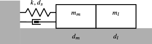
A representation of a PEA coupled with an inertial load.

4. Analysis of Parallel Elastic Actuators
PEAs often consist of electromagnetic motors which have their stator fixed to ground and their rotor connected to a spring, with the opposite end of the spring connected to the ground [Reference Verstraten, Beckerle, Furnémont, Mathijssen, Vanderborght and Lefeber14, Reference Beckerle, Verstraten, Mathijssen, Furnémont, Vanderborght and Lefeber15]. The rotor is also rigidly connected to a link or to a load as represented in Fig. 2 where angular variables are converted into linear equivalents. The mass
 $m_{m}$
represents the rotor inertia,
 $m_{l}$
is the link, and k is the spring stiffness. Dissipation sources may be located between the rotor and stator, such as the damping due to bearings or brushes, in parallel to the spring, due to non ideal elastic behavior and on the load, representing dissipations due to the environment. These dissipation sources are characterized here by the damping coefficients
 $d_{m},\;d_{s}$
and
 $d_{l}$
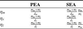
. The motor transmission is considered fully backdrivable. The notation used in this section and in the following is summarized in Table I. Defining
 $M=m_{m}+m_{l}$
and
 $D=d_{m}+d_{s}+d_{l}$
, the system dynamics can be expressed as
 \begin{equation}M\ddot{x}_{l}(t)+D\dot{x}_{l}(t)+kx_{l}(t)=F(t).\end{equation}
where
 $x_{l}$
is the load position. It follows that the input that exactly compensates for dissipation is
 $F(t)=D\dot{x}_{l}(t)$
. By applying this input and by choosing initial conditions
 $x_{l}(0)=0$
and
 $\dot{x}_{l}(0)=\alpha\omega_{P}$
, where
 $\omega_{P}=\sqrt{\frac{k}{M}}$
is the resonance frequency of the PEA, we have the following state trajectories
 \begin{align} x_{l}(t) =\alpha\sin(\omega_{P}t) \end{align}
 \begin{align} \dot{x}_{l}(t) =\alpha\omega_{S}\cos(\omega_{P}t) \end{align}
which describes a resonant motion. Thus, the system (12) oscillates at its natural frequency with constant resonant energy
 $E_{r}$
 \begin{equation}E_{r}=K+U=\frac{1}{2}M\dot{x}_{l}(t)^{2}+\frac{1}{2}kx_{l}(t)^{2}=\frac{1}{2}k\alpha^{2}\end{equation}
where K and U are kinetic and potential energy. The dissipated power is
 $P_{dis}=D\dot{x}_{l}^{2}(t)$
which can be averaged over the period
 $T=2\pi/\omega_{S}$
leading to
 \begin{equation}\bar{P}_{dis,r}=\frac{1}{T}\int_{0}^{T}D\dot{x}_{l}^{2}(t)dt=\frac{Dk\alpha^{2}}{2M}\end{equation}
where
 $\dot{x}_{l}$
has been substituted as in (13b). Then, we can compute the index
 $\eta$
as
 \begin{equation}\eta=\frac{E_{r}}{\bar{P}_{dis,r}}=\frac{M}{D}=\frac{m_{m}+m_{l}}{d_{m}+d_{s}+d_{l}}.\end{equation}
We observe from (16) that the motion magnitude
 $\alpha$
is canceled out, as anticipated in the previous section. As the PEA model (12) is second order, it exhibits a single (resonant) mode. Consequently, all the internal energy is stored in this resonant mode and no temporary energy is present in the system. In this case
 \begin{equation}\eta=\eta^{TE}=\eta^{WC}.\end{equation}
System parameters.

A representation of a SEA coupled with an inertial load.

5. Analysis of Series Elastic Actuators
In typical SEA architectures, the stator of the motor is fixed to ground and the rotor is connected to the link or to the load by means of an elastic element. This is represented in Fig. 3 where, again, angular variables are converted into linear equivalents. The mass
 $m_{m}$
represents the rotor inertia with position
 $x_{m}$
and
 $m_{l}$
is the link or load inertia with position
 $x_{l}$
. The elastic element in between is characterized by stiffness k and damping
 $d_{s}$
and the motor transmission is considered fully backdrivable. Other dissipation sources are located between the rotor and stator (
 $d_{m}$
) and on the load (
 $d_{l}$
). The resulting system dynamics are
 \begin{align} m_{m}\ddot{x}_{m} =F-d_{m}\dot{x}_{m}-k(x_{m}-x_{l})-d_{s}(\dot{x}_{m}-\dot{x}_{l}) \end{align}
 \begin{align} m_{l}\ddot{x}_{l} =-d_{l}\dot{x}_{l}+k(x_{m}-x_{l})+d_{s}(\dot{x}_{m}-\dot{x}_{l}) \end{align}
where
 $x_{m}$
is the motor position,
 $x_{l}$
is the load position and time dependency of
 $x_{m}(t)$
,
 $x_{l}(t)$
and F(t) is omitted for space reasons. The SEA model (18a)-(18b) is fourth order which, in modal coordinates, results in one oscillatory mode and one translatory mode.Footnote 4 Consequently, when the system is excited at its natural frequency, the oscillatory mode stores the resonant energy while some temporary energy may flow in the translatory mode. In contrast to PEAs, damping parameters cannot be aggregated and each dissipation source is analyzed separately in the following sections.
5.1. Motor damping
Similarly to the case of PEA, motor damping can be compensated by positing
 $F(t)=d_{m}\dot{x}_{m}(t)$
which leads to the following system dynamics
 \begin{align} m_{m}\ddot{x}_{m}(t) =-k(x_{m}(t)-x_{l}(t)) \end{align}
 \begin{align} m_{l}\ddot{x}_{l}(t) = k(x_{m}(t)-x_{l}(t)) \end{align}
which exhibits a resonant frequency in
 \begin{equation}\omega_{S}=\sqrt{\frac{k}{m_{m}}+\frac{k}{m_{l}}.}\end{equation}
In order to observe the system during a resonant motion, we consider the initial conditions
 $x_{m}(0)=x_{l}(0)=0,\:\dot{x}_{m}(0)=\alpha\omega_{S}\mu$
and
 $\dot{x}_{l}(0)=-\alpha\omega_{S}$
leading to the following motion equations
 \begin{align} x_{m}(t) & =-\mu\alpha\sin(\omega_{S}t) \end{align}
 \begin{align} \dot{x}_{m}(t) & =-\mu\alpha\omega_{S}\cos(\omega_{S}t)\end{align}
 \begin{align} x_{l}(t) & =\alpha\sin(\omega_{S}t)\end{align}
 \begin{align} \dot{x}_{l}(t) & =\alpha\omega_{S}\cos(\omega_{S}t)\end{align}
where
 $\mu=m_{l}/m_{m}$
. The internal energy can be computed by considering
 \begin{align} K & =\frac{1}{2}m_{m}\dot{x}_{m}^{2}+\frac{1}{2}m_{l}\dot{x}_{l}^{2}=\frac{1}{2}\alpha^{2}\omega_{S}^{2}m_{l}(1+\mu)\cos^{2}\omega_{S}t \end{align}
 \begin{align} U & =\frac{1}{2}k(x_{m}-x_{l})^{2}=\frac{1}{2}\alpha^{2}k(1+\mu)^{2}\sin^{2}\omega_{S}t\end{align}
which leads to
 \begin{equation}E=U+K=\frac{1}{2}\alpha^{2}k(1+\mu)^{2}.\end{equation}
Thus, the total internal energy E is constant over time and is completely stored in the resonant mode. As a consequence, no temporary energy arises.Footnote 5 The mean dissipated power for damping compensation can be expressed as
 \begin{equation}\bar{P}_{d_{m}}=d_{m}\frac{1}{T}\int_{0}^{T}\dot{x}_{m}^{2}(t)dt\end{equation}
where
 $T=2\pi/\omega_{S}$
. Considering that
 $\frac{1}{T}\int_{0}^{T}\sin^{2}\omega_{S}t=\frac{1}{2}$
, we have
 \begin{equation}\bar{P}_{d_{m}}=\frac{1}{2}d_{m}\mu^{2}\alpha^{2}\omega_{S}^{2}=\frac{1}{2}\alpha^{2}k\frac{\mu(1+\mu)}{m_{m}}d_{m}\end{equation}
and we can finally compute the index
 \begin{equation}\eta_{m}=\frac{E_{r}}{\bar{P}_{d_{m}}}=\frac{m_{m}+m_{l}}{d_{m}}\frac{m_{m}}{m_{l}}.\end{equation}
5.2. Spring damping
When the damping is located in the spring, it is convenient to explicitly distinguish between the resonant and the translatory modes. To this aim, the SEA model (18a)-(18b) can be expressed in modal coordinates as
 \begin{align} z_{1} = m^{-1}(\mu x_{l}+x_{m}) \end{align}
 \begin{align} z_{2} = m^{-1}(x_{l}-x_{m})\end{align}
where
 $m=1+\mu$
, leading to the modal representation
 \begin{equation}M_{p}\left[\begin{array}{c}\ddot{z}_{1}\\\ddot{z}_{2}\end{array}\right]+D_{p}\left[\begin{array}{c}\dot{z}_{1}\\\dot{z}_{2}\end{array}\right]+K_{p}\left[\begin{array}{c}z_{1}\\z_{2}\end{array}\right]=\left[\begin{array}{c}F\\-\mu F\end{array}\right]\end{equation}
where
 \begin{eqnarray}M_{p} & = & \left[\begin{array}{cc}mm_{m} & 0\\0 & mm_{l}\end{array}\right],\end{eqnarray}
 \begin{eqnarray}D_{p} & = & \left[\begin{array}{cc}d_{m}+d_{l} & d_{l}-\mu d_{m}\\d_{l}-\mu d_{m} & m^{2}d_{s}+\mu^{2}d_{m}+d_{l}\end{array}\right],\end{eqnarray}
 \begin{eqnarray}K_{p} & = & \left[\begin{array}{cc}0 & 0\\0 & m^{2}k\end{array}\right].\end{eqnarray}
Here the states
 $z_{1}$
and
 $\dot{z}_{1}$
describe the translatory mode while
 $z_{2}$
and
 $\dot{z}_{2}$
represent the resonant mode. The modal transformation (31a)-(31b) is energy preserving and allows to easily distinguish the resonant energy, stored in states
 $z_{2}$
and
 $\dot{z}_{2}$
, from the temporary energy, stored in states
 $z_{1}$
and
 $\dot{z}_{1}$
.
If we consider a single dissipation source given by
 $d_{s}$
, the damping matrix
 $D_{p}$
is diagonal and the Eqs. (32) become decoupled:
 \begin{align} mm_{m}\ddot{z}_{1} =F \end{align}
 \begin{align} mm_{l}\ddot{z}_{2}+m^{2}d_{s}\dot{z}_{2}+m^{2}kz =-\mu F. \end{align}
Focusing on the latter row we can impose
 \begin{equation}F=-\frac{m^{2}}{\mu}d_{s}\dot{z}_{2}=\frac{1+\mu}{\mu}(x_{m}-x_{l})\end{equation}
to have perfect damping compensation. Similarly as before, initial conditions can be chosen on order to observe the following resonant motion
 \begin{align} z_{2}(t) & =\alpha\sin(\omega_{S}t) \end{align}
 \begin{align} \dot{z}_{2}(t) & =\alpha\omega_{S}\cos(\omega_{S}t) \end{align}
which implies a constant level of resonant energy
 \begin{equation}E_{r}=K_{2}+U_{2}=\frac{1}{2}mm_{l}\dot{z}_{2}^{2}+\frac{1}{2}m^{2}kz^{2}=\frac{1}{2}\alpha^{2}m^{2}k.\end{equation}
The average power needed for damping compensation can be computed from (35) as
 \begin{equation}\bar{P}_{d_{s},r}=m^{2}d_{s}\frac{1}{T}\int_{0}^{T}\dot{z}_{2}^{2}(t)dt=\frac{1}{2}\alpha^{2}m^{3}k\frac{d_{s}}{m_{l}}\end{equation}
and finally we have
 \begin{equation}\eta_{s}=\frac{E_{r}}{\bar{P}_{d_{s}}}=\frac{m_{l}}{md_{s}}=\frac{m_{m}m_{l}}{m_{m}+m_{l}}\frac{1}{d_{s}}.\end{equation}
5.2.1. Accounting for Temporary Energy
By substituting (35) in (34a) we find that, in order to compensate for
 $d_{s}$
, some energy is introduced in the mode
 $z_{1}$
leading the two masses to oscillate in-phase. Unfortunately, the system cannot permanently store this energy because, as reported in (34a) the mode
 $z_{1}$
exhibits pure integrator dynamics. The temporary energy is just temporarily stored in the state
 $\dot{z}_{1}$
as kinetic energy and then exits the system as negative input power. In particular, given the input (35) and a proper choice of initial conditions, we can solve Eq. (34a) and compute
 \begin{equation}\dot{z}_{1}=-\alpha\frac{m}{m_{l}}d_{s}\sin\omega_{S}t.\end{equation}
The associated kinetic energy is
 \begin{equation}K_{1}=\frac{1}{2}mm_{m}\dot{z}_{1}^{2}=\frac{1}{2}\alpha^{2}\frac{m^{3}}{\mu m_{l}}d_{s}^{2}\sin^{2}\omega_{S}t\end{equation}
which increases in the first quarter of the period and decreases in the second quarter. In a half period (
 $T/2$
) such temporary energy is released as negative input power which may be dissipated by the motor driver. Such dissipated power can be computed by relating the released energy with the releasing period
 $T/2$
leading to
 \begin{equation}\bar{P}_{d_{s},tA}^{WC}=\frac{\max(K_{1})}{T/2}=f\alpha^{2}\frac{m^{3}}{\mu m_{l}}d_{s}^{2}\end{equation}
where
 $f=1/T=\omega_{S}/2\pi$
is the resonance frequency of the SEA and
 $\omega_{S}$
is defined in (20). It is worth highlighting that such dissipated power is related to worst case condition. Indeed, the amount of temporary energy is reduced when the load inertia
 $m_{l}$
is constrained by some downstream dynamics. For example, in the limit case of fixed load inertia there will be no temporary energy because no in-phase oscillation can occur. In contrast, when the load mass is completely unconstrained, we have the highest temporary energy and higher associated dissipated power which represents the worst case condition (WC) for efficiency. The worst case index can be computed considering such worst case dissipated power as
 \begin{equation}\eta_{s}^{WC}=\frac{E_{r}}{\bar{P}_{d_{s},tA}^{WC}}=\frac{\eta_{s}}{1+\frac{fd_{s}}{\mu k}}\end{equation}
or equivalently as
 \begin{equation}\eta_{s}^{WC}=\frac{\eta_{s}}{1+\sigma d_{s}},\quad\sigma=\frac{m_{m}}{m_{l}\sqrt{k\cdot m_{m}||m_{l}}}\end{equation}
where the notation
 $m_{m}\parallel m_{l}$
indicates the parallel of motor and load inertias
 $m_{m}\parallel m_{l}=\frac{m_{m}m_{l}}{m_{m}+m_{l}}$
. This index accounts for dissipation of type A, while dissipation of type B is not observed because no dissipation term related to state
 $\dot{z}_{1}$
exists in Eqs. (34a)-(34b). By looking at the coefficient
 $\sigma$
it seems that such dissipation (type A) increases when the motor inertia is high and at the same time the load inertia is low. Also, it decreases with the actuator stiffness. Thus, rigid systems which avoid the combination of high motor inertia and lightweight load seem to be more efficient in the sense that they are less prone to dissipation due to the temporary energy.
5.3. Load damping
In the case of load damping we can consider the following modal equations
 \begin{align} mm_{m}\ddot{z}_{1} +d_{l}\dot{z}_{1}+d_{l}\dot{z}_{2}=F \end{align}
 \begin{align} mm_{l}\ddot{z}_{2} +d_{l}\dot{z}_{1}+d_{l}\dot{z}_{2}+m^{2}kz_{2}=-\mu F \end{align}
with states
 $\dot{z}_{2},\:z_{2}$
representing the oscillatory mode and
 $\dot{z}_{1},\:z_{1}$
the translatory mode. In this case both system modes are involved in energy dissipation, leading to type B dissipation. Focusing on (46b), damping terms can be compensated by imposing
 $F=-\frac{d_{l}}{\mu}(\dot{z}_{1}+\dot{z}_{2})=-\frac{d_{l}}{\mu}\dot{x}_{l}$
which lets the system oscillate at its natural frequency. The system dynamics then becomes
 \begin{align} m_{m}\ddot{z}_{1} +d_{l}\dot{z}_{1}+d_{l}\dot{z}_{2}=0 \end{align}
 \begin{align} m_{l}\ddot{z}_{2} +mkz_{2}=0. \end{align}
Similarly to previous sections, initial conditions can be chosen on order to observe the following resonant motion
 \begin{align} z_{2}(t) =\alpha\sin(\omega_{S}t)\end{align}
 \begin{align} \dot{z}_{2}(t) =\alpha\omega_{S}\cos(\omega_{S}t). \end{align}
The resonant energy is stored in the states
 $\dot{z}_{2},\:z_{2}$
and can be computed as in the previous section
 \begin{equation}E_{r}=\frac{1}{2}\alpha^{2}m^{2}k.\end{equation}
If we neglect the temporary energy by considering
 $z_{1}=\dot{z}_{1}=0$
, the average dissipated power is
 \begin{equation}\bar{P}_{d_{l},r}=d_{l}\frac{1}{T}\int_{0}^{T}\dot{z}_{2}^{2}(t)dt=\frac{1}{2}\alpha^{2}\omega_{S}^{2}d_{L}\end{equation}
and the index
 $\eta_{l}$
can be expressed as
 \begin{equation}\eta_{l}=\frac{E_{r}}{\bar{P}_{d_{l},r}}=\frac{m_{m}+m_{l}}{d_{l}}\frac{m_{m}}{m_{l}}.\end{equation}
5.3.1. Accounting for Temporary Energy
When compensating for load damping, we have dissipation of both type A and B. The first is due to the temporary energy exiting the system as negative input power (and then being dissipated by the motor driver). The second is due to the dissipative terms
 $d_{l}\dot{z}_{1}$
in (46a) and (46b). As before, to characterize the worst case dissipation, the trajectory of
 $z_{1}$
is computed by considering an unconstrained load. In particular, Eq. (47a) can be solved in the Laplace domain by replacing
 $z_{2}$
with its transform leading to
 \begin{equation}z_{1}(s)=\frac{-\alpha\gamma\omega_{S}}{(s+\gamma)(s^{2}+\omega_{S}^{2})}\end{equation}
where
 $\gamma=\frac{d_{l}}{m_{l}}$
. Then by anti-transformation and proper choice of initial conditions it is possible to express
 $z_{1}$
as
 \begin{equation}z_{1}(t)=\frac{-\alpha}{\gamma^{2}+\omega_{S}^{2}}(\gamma\omega_{S}e^{-\gamma t}+\gamma\omega_{S}\cos\omega_{S}t+\gamma^{2}\sin\omega_{S}t).\end{equation}
The exponential term just represents a transient and is neglected from here on. The power within system modes can be computed as
 $P_{d_{l}}+P_{d_{l}}^{WC-B}=d_{l}(\dot{z}_{1}+\dot{z}_{2})^{2}$
. It also accounts for type B dissipation due to the worst case temporary energy. The trajectory
 $\dot{z}_{1}$
can be derived from (53) as
 \begin{equation}\dot{z}_{1}(t)=\frac{\alpha}{\gamma^{2}+\omega_{S}^{2}}(\gamma^{2}\omega_{S}\cos\omega_{S}t-\gamma\omega_{S}^{2}\sin\omega_{S}t)\end{equation}
while
 $\dot{z}_{2}$
is expressed in (48b). By defining
 $h=\frac{\omega_{S}^{2}}{\gamma^{2}}=\frac{kmm_{l}}{d_{l}^{2}}$
, the dissipated power can be computed as
 \begin{equation}P_{d_{l},r}+P_{d_{l},tB}^{WC}=d_{_{l}}\alpha^{2}\left(\frac{h+2}{h+1}\omega_{S}\cos\omega_{S}t-\frac{h}{h+1}\gamma\sin\omega_{S}t\right)^{2}\end{equation}
and on average we have
 \begin{equation}P_{d_{l},r}+P_{d_{l},tB}^{WC}=\frac{1}{2}\alpha^{2}\omega_{S}^{2}(1+3\xi)d_{l}\end{equation}
where
 $\xi=\frac{1}{h+1}$
. The efficiency index accounting for worst case type B dissipations can be computed as
 \begin{equation}\eta_{l}^{WC-B}=\frac{E_{r}}{P_{d_{l},r}+P_{d_{l},tB}^{WC}}=\frac{m_{m}+m_{l}}{d_{l}}\frac{m_{m}}{m_{l}}\frac{1}{(1+3\xi)}.\end{equation}
Again, this index is worst case because the load mass is unconstrained, leading to the maximum temporary energy flowing into the system (maximum in-phase oscillations). As we are not yet accounting for type A dissipations,
 $\eta_{l}^{WC-B}$
describes the case of a system capable of recovering the negative input power. We can say that a SEA with an energy recovery circuit can exhibit an efficiency index with a value between
 $\eta_{l}$
in (51), where the temporary energy was entirely neglected, and
 $\eta_{l}^{WC-B}$
in (57), depending on the load/environment dynamics. Interestingly, the ratio between
 $\eta_{l}$
and
 $\eta_{l}^{WC-B}$
is given by the coefficient
 $\frac{1}{(1+3\xi)}$
which can reduce the worst case efficiency by no more than a quarter. Indeed, since
 $h>0$
, one has that
 $0\leq\xi\leq1$
. When k is high the quantity
 $\xi$
is small and we again find that a series elastic system with high stiffness leads to higher efficiency in resonant motions, because the temporary energy flow is minimized. A similar effect can be observed for high load and low motor inertia.
Finally, to compute type A dissipation we need to consider the negative input power dissipated by the motor driver in absence of an energy recovery circuit. As in previous section
 $\bar{P}_{d_{l},tA}^{WC}$
is given by the kinetic energy which is temporarily stored in the state
 $\dot{z}_{1}$
and then released
 \begin{align} K_{1} =\frac{1}{2}mm_{m}\dot{z}_{1}^{2} \end{align}
 \begin{align} =\frac{1}{2}mm_{m}\alpha\omega^{2}\left[\frac{1}{h+1}\cos\omega_{S}t-\frac{h}{h+1}\sin\omega_{S}t)\right]^{2}.\end{align}
The negative input power can be computed as before considering the amount of released energy
 $\max(K_{1})$
within the releasing period
 $T/2$
. After some small computationsFootnote 6 this leads to
 \begin{equation}\bar{P}_{d_{l},tA}^{WC}=\frac{\max(K_{1})}{T/2}=\frac{1}{2}\alpha^{2}f\frac{mm_{m}}{m_{^{2}}}d_{l}^{2}(1-\xi)\end{equation}
and the worst case efficiency index in absence of an energy recovery circuit is
 \begin{align} \eta_{l}^{WC} =\frac{E_{r}}{P_{d_{l},r}+P_{d_{l},tB}^{WC}+P_{d_{l},tA}^{WC}} \end{align}
 \begin{align} =\frac{\eta_{l}}{1+\sigma d_{l}(1-\xi)+3\xi}. \end{align}
Interestingly, when
 $\xi=0$
Eq. (60a) reduces to the following expression
 \begin{equation}\eta_{l}^{WC}=\frac{\eta_{l}}{1+\sigma d_{l}}\end{equation}
which is similar to the case of spring damping (45).
6. Discussion of Analytical Results
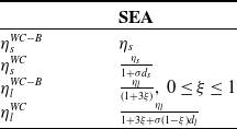
To summarize our findings, Table II reports the index
 $\eta$
for PEAs and SEAs, distinguishing the cases of motor, spring and load dissipation. These expressions completely neglect the temporary energy, possibly leading to an overestimation of
 $\eta_{s}$
and
 $\eta_{l}$
in the SEA case. Table III reports the associated correction terms when accounting for the maximum (worst case) flux of temporary energy, arising when the load inertia is unconstrained. Indices
 $\eta_{s}^{WC}$
and
 $\eta_{l}^{WC}$
consider a scenario of temporary energy dissipation within motor drivers, while
 $\eta_{s}^{WC-B}$
and
 $\eta_{l}^{WC-B}$
consider the availability of an energy recovery circuit, thus they only account for type B dissipation. In the case of spring damping, type B dissipation does not occur, thus
 $\eta_{s}^{WC-B}=\eta_{s}$
. In this case, once the temporary energy is recovered, its net contribution is becomes null. The same does not hold in the case of load damping.
Overview of Computed Indices

Correction Terms due to Temporary Energy

The overall energy consumption arising from the combination of different sources can be computed by simply adding the related “inefficiencies” as
 \begin{equation}\frac{1}{\eta}=\frac{1}{\eta_{m}}+\frac{1}{\eta_{s}^{*}}+\frac{1}{\eta_{l}^{*}}\end{equation}
where the apex
 $*$
means that, depending on the scenario, the terms in Table III can be used instead of the ones in Table II. Equation (62) can easily be derived considering that all the indices in Tables III and II share the same numerator,
 $E_{r}$
.
We observe that all the indices reported in Table II are proportional to inertial quantities and inversely proportional to damping parameters. Given the same damping, the larger the inertia is, the more the system is inclined to preserve internal energy and its resonant motion as a consequence. Returning to the example of PDWs, a walker with high inertia is expected to exhibit longer lasting motion with respect to a lighter one, thanks to its higher kinetic energy storage capabilities (assuming similar damping coefficients for both walkers). A second observation is that the index
 $\eta$
(4) can be related to the COT (3) to define the efficiency of a transportation task. In particular, if we consider the transportation of a load with mass m and damping d, we have
 \begin{equation}COT=\frac{dv^{2}}{mgv}\end{equation}
where v is the transportation velocity. Such an inertial system with mass m and damping d can be modeled as a second-order system with a pure integrator. The index
 $\eta$
as defined in (4) can then be computed following the methodology described in Section 3, resulting in
 $\eta=m/d$
. In this case the system exhibits a single translatory mode which represents the “resonant” modeFootnote 7 and the velocity v represents the amplitude of the translatory motion. Thus, we have
 \begin{equation*}COT=\frac{v}{\eta g}\end{equation*}
where we can distinguish system-related parameters, m and d, both embedded in
 $\eta$
, the task-related parameter v, and the constant g. As stated in Section I,
 $\eta$
describes the system efficiency in terms of system parameters and independently from the specific task characterized by v. Thus, disregarding the task, the system efficiency (or inefficiency) expressed by the COT can be equivalently expressed using the proposed index
 $\eta$
. This finding supports the general validity of our analysis.
7. Validation
To validate the consistency of the proposed analysis and the accuracy of the indices in Tables II and III, we compare them with energy consumption measures in a simulation scenario and validate them in a physical environment.
7.1. Simulation Validation
In our simulations, we consider a scenario where the load is unconstrained (maximum temporary energy) and no energy recovery circuit is available. This can be considered as a worst case scenario for the SEA, because in several applications the load is somehow constrained. For example, if we consider a legged robot with the robot’s foot as a load, we find that the foot is constrained to the ground during the stance phase, and it is constrained by gravity forces during other phases. Similarly, if we consider pick-and-place applications, dynamic constraints due to gravity apply. A set of inertial (
 $m_{m},\:m_{l}$
) and damping (
 $d_{m},\:d_{s},\:d_{l}$
) parameters are considered while the spring stiffness (k) is fixed. The set of inertial parameters ranges from
 $10^{-4}\;Kgm^{2}$
to
 $1\;Kgm^{2}$
and includes typical values of rotor reflected inertias, representative of a wide set of electromagnetic gear-motors, from direct-drive to high gear-ratio. Similarly, we impose realistic damping values in the range of
 $(10^{-3},10^{-2})\;Nm/rad$
. The stiffness parameter is set to
 $k=100\;Nm/rad$
and represents a typical choice for SEAs whose stiffness ranges from some tens to some hundreds of
 $Nm/rad$
. We chose to fix this value as the efficiency index
 $\eta$
do not depend on k, as reported in Table II
The following damping compensation laws are implemented
 \begin{align} F_{PEA} & =\left(d_{m}+d_{s}+d_{l}\right)\dot{x}_{l}(t) \end{align}
 \begin{align} F_{SEA} & =\left(d_{m}+\frac{1+\mu}{\mu}d_{l}\right)\dot{x}_{m}(t)-\left(\frac{1+\mu}{\mu}d_{s}+\frac{1}{\mu}d_{l}\right)\dot{x}_{l}(t)\end{align}
for the case of PEA and SEA, as derived in the analysis in sections 4 and 5.
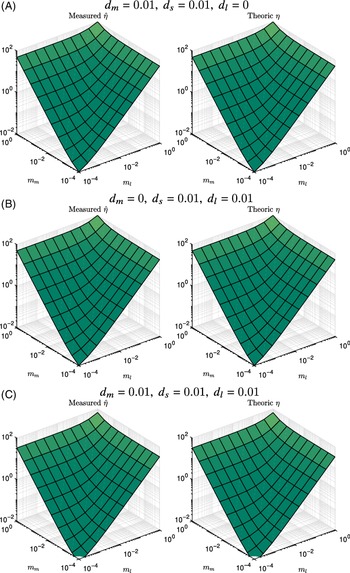
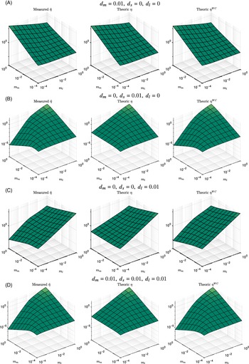
Comparison between measured (left) and analytical (right) efficiency indices for PEAs.

Comparison between measured (left column) and theoretic indices for SEAs.

Efficiency is measured according to (9) as
 \begin{equation}\hat{\eta}=E_{r}/mean(P_{in}^{+}(t))\end{equation}
where
 $P_{in}^{+}$
represents the power flowing from the driver to the motor (which is dissipated in the mechanical domain) plus the power flowing back from the motor to the driver (which is dissipated within the motor driver, as a recovery circuit is not included). More specifically,
 $P_{in}^{+}(t)$
is computed as the absolute value
 $P_{in}^{+}(t) = |\dot{x}_{m}(t)F(t)|$
where
 $\dot{x}_{m}$
and F represent the motor velocity and the motor input force or torque, proportional to the current.
Figure 4 shows, for the case of PEA, the measured index
 $\hat{\eta}$
against the index
 $\eta$
analytically computed as in Table II. One can observe that measured and theoretic plots present the same shape. The maximum relative error between the two is quantified as 0.264%. Logarithmic scales on the X and Y axes are chosen in order to span very different values of
 $m_m$
and
 $m_l$
. Similarly, we choose logarithmic scales on the Z axis in order to highlight differences between measured and theoretic indices, as the efficiency indices span very different magnitudes. Figure 5 shows the same results for the case of SEA. Here the measured values are compared with the proposed indices, either accounting or not accounting for the effects of temporary energy. As expected, the measured efficiency presents the same shape of the worst case index
 $\eta^{WC}$
. This is not because the index
 $\eta^{WC}$
is more accurate, but because we simulated worst case scenarios (maximum temporary energy). We highlight that on a linear scale the discrepancy of indices
 $\eta$
and
 $\eta^{WC}$
would be not significant, as we show here after. Nevertheless, the proposed indices are able to capture even small differences and show consistency with measured efficiency even on a logarithmic scale. We can conclude that, both for PEA and SEA, the measured efficiency agrees with our theoretical expectations, thus validating our theoretical analysis.
Before proceeding, we highlight some particularities regarding the case of SEA. First, the difference between indices
 $\eta$
and
 $\eta^{WC}$
on a linear scale is extremely small. To make it noticeable, we needed to apply an extremely low value for the stiffness
 $k=1\: Nm/rad$
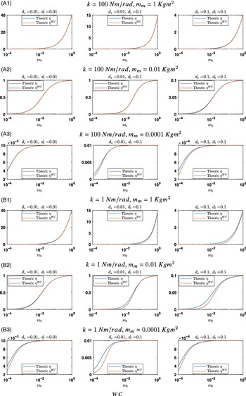
– outside of the typical stiffness value ranges for SEA designs – and high distal friction values. These results are reported in Figure 6, where a linear scale is used for the Y axis. In these plots, we avoid showing the measured efficiency as it would overlap with
 $\eta^{WC}$
(as reported in Figure 5). Three different values are considered for
 $m_m$
and two for k. Even if
 $\eta$
and
 $\eta^{WC}$
are very close to each other, some differences can be observed in case of high distal friction. This agrees with the equations reported in Table III. Also, by comparing the first three rows A1, A2, and A3 – where we considered a stiffness
 $k=100\: Nm/rad$
– with the last three rows B1, B2 and B3 – where we considered a very low stiffness
 $k=1\: Nm/rad$
– one can observe that
 $\eta^{WC}$
decreases, leading to more noticeable differences. This is because
 $\eta^{WC}$
depends on
 $\sigma$
and
 $\xi$
which in turns depends on k. Instead,
 $\eta$
does not change with k as reported in Table II. Thus, if we neglect the (small) temporary energy dissipation, we can state that k affects the resonance frequency location, but not the efficiency magnitude. Finally, we highlight that even if the plots reported in Figure 5 for the SEA show a maximum discrepancy between
 $\eta$
and
 $\eta^{WC}$
for high
 $m_m$
and low
 $m_l$
, this is not a general result. This is just due to the combination of two choices: the considered parameter set and the logarithmic scale, as can be observed by comparing Figures 5 and 6.
Comparison between indices
 $\eta$
and
 $\eta^{WC}$
on linear scales, for SEAs with increasing values of parameters
 $d_s$
and
 $d_l$
and for different values of
 $m_m$
.

7.2. Experimental Validation
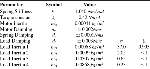
In the previous section, an extensive validation has been provided in simulation, considering a wide set of inertia parameters. Since it is not practically feasible to test many mechanical arrangements in experiments, we choose to experimentally validate the few scenarios representing the more complex conditions highlighted by the proposed methodology. In particular, this section proposes an experimental validation considering the case of a SEA with different lightweight loads. The experimental setup consists of the elastic actuator prototype in figure 7. It is composed of a direct drive torque motor M connected in series to a spring S (used in torsional mode) and to an exchangeable load L. System parameters have been estimated using a procedure similar to the one described in ref. [Reference Calanca, Capisani, Ferrara and Magnani53] and are reported in Table IV, where
 $m_{li}$
for
 $i=1...4$
refers to different load inertias. As the inherent mechanical damping is low, we used a soft spring in order to obtain noticeably differences between indices
 $\eta$
and
 $\eta^{WC}$
as discussed in the previous section. For each load, Table III reports the parameters
 $\xi$
and
 $\sigma$
defined in (56) and (45). The motor Coulomb friction is compensated using a
 $\mathrm{sign}(\dot{x}_{m})$
function and neglected because its nonlinear nature is not considered in our analysis. Static and stick-slip friction are not compensated because of their complex dynamics.
Parameters of the Experimental Setup

The SEA prototype used as testbed.

Two optical encoders E1 and E2 are used to measure motor and load position, respectively. They are connected to an industrial rack that drives a motor current amplifier and provides an EtherCat connection to a standard PC on which the control algorithm runs. No energy recovery system is present in the motor driver.
In our analysis, we assume the resonant energy is maintained by perfect damping compensation. However, it is very challenging to obtain perfect damping compensation in the real world. Static and stick-slip friction dynamics are hard to model and estimation of system parameter may suffer some bias. Thus, in practice, friction and damping forces will always be either overestimated or underestimated, resulting in either an increase or a decrease in the initial system energy. To keep the internal energy constant, we therefore relied on an energy-based control approach. Energy control injects power into the system until a desired level
 $E_{d}$
of internal energy E is reached. This strategy has been used for example to control PDWs [Reference Spong and Bhatia54]. According to [Reference Spong and Bhatia54] energy control can be formulated as
 \begin{eqnarray}F(t) & = & k_{e}(E_{d}-E(t))\dot{x}_{m}(t)\end{eqnarray}
where
 $k_{e},$
is a control gain and E is the overall system energy. One can observe that the input power
 $P_{in}(t)=F(t)\dot{x}_{m}(t)$
is positive when the system’s energy E is below the energy target
 $E_{d}$
and negative otherwise. The stability of the control law (67) can be proven considering E(t) as a Lyapunov function candidate, as in ref. [Reference Spong and Bhatia54]. In the case of SEA, E(t) can be computed as
 \begin{equation}E=U+K=\frac{1}{2}m_{m}\dot{x}_{m}^{2}+\frac{1}{2}m_{l}\dot{x}_{l}^{2}+\frac{1}{2}k(x_{m}-x_{l})^{2}.\end{equation}
However, as the control law (67) may inject power in both the resonant and translatory modes, a slightly modified version is proposed here, to minimize the effect of temporary energy:
 \begin{equation}F(t)=k_{e}(E_{d}-E(t))\dot{z}_{2}(t)\end{equation}
The difference between (67) and (69) is that the latter injects energy directly on the state
 $\dot{z}_{2}$
which stores the resonant energy. Nothing prevents some energy from being injected into the state
 $\dot{z}_{1}$
as a side effect but in minor part in comparison to (67). It can be proven that the energy control law (69) implicitly acts like a damping compensation law and its stability can be proven considering
 $E_{r}(t)$
, as expressed in (38), as a candidate Lyapunov function (proof is beyond the scope of this paper). Typical energy trends can be observed in Figure 8. After transients, the resonant energy
 $E_{r}$
reaches an almost constant value, while the temporary energy
 $E_{t}$
is still oscillating, alternating between energy accumulation and energy release phases, as expected. Power trends are reported in the lower plot where
 $P_{in}$
represents the input power and
 $P_{dis}=P_{dis,r}+P_{dis,tB}$
the power dissipated within the system, in both resonant and nonresonant modes.
Energy and power trends in SEA simulation using energy control as in (67).

Data have been collected in 24 experiments characterized by 4 different loads, with different inertia, and with 6 different oscillation amplitudes corresponding to 6 different values for
 $E_{d}$
in (67). Figure 9 reports the measured efficiency in comparison with the analytical expectations, including worst case expectations as we did for the simulation results (Figures 4 and 5). The main differences in comparison with the simulation are that (1) the motor inertia is not changed, leading to a two-dimensional plot similar to those in Figure 6 instead of a three-dimensional one; (2) some noise can be observed in the measured index
 $\hat{\eta}$
, probably due to stiction effects, shaft misalignment and cogging torques, which can influence the experimental outcome depending on the motion amplitude and on the initial experimental conditions. In particular, stiction effects may present a dynamic constraint on the load, possibly affecting the temporary energy level. In the case of higher load inertias, one can see an agreement between the measured efficiency
 $\hat{\eta}$
and the analytical index
 $\eta$
. For the lowest load inertia, the index
 $\eta$
– which neglects the temporary energy – overestimates the system efficiency which lies between
 $\eta$
and
 $\eta^{WC}$
, as expected. This is observed only for the lowest load inertia because this situation involves higher levels of temporary energy, in accordance with (44) and (60a).
SEA experimental validation: measured
 $\hat{\eta}$
in comparison with theoretic expectations
 $\eta$
and
 $\eta^{WC}$
.

7.3. Discussion
The results from our simulations and experiments uncover some guidelines for the efficient design of elastic actuators, which we will discuss in this section. First of all, we can state that SEAs and PEAs are characterized by different energetic behaviors. Our analysis and results show that, due to the temporary energy, SEAs are affected by additional dissipation with respect to PEAs. This is because (a) the temporary energy is not recovered and (b) the temporary energy implies additional motion, which results in additional dissipation. However, by simulating the SEA system considering a wide set of realistic parameter values, we found that such additional dissipation should be quite low in practice. Even in our experimental validation, we could see the effects of temporary energy only by choosing extremely low spring stiffness k and load inertia
 $m_{l}$
. This agrees with equations (45) and (60a). However, it must be noted that higher temporary energy dissipation can show up in the case of high distal friction,, high values for
 $d_{s}$
and
 $d_{l}$
as shown in Figure 6. It may thus be convenient to minimize these dissipation sources. Instead, motor friction was not found to be linked to temporary energy.
Beside the dissipation due to temporary energy, some distinct characteristics of SEA and PEA efficiency can be observed. A comparison of figures 4 and 5 reveals that PEAs behave more efficiently than SEAs in some conditions. This applies in particular when the either the motor or the load inertia are high. The case of SEAs is more controversial. In particular, in the case of high dissipation in the motor, SEAs retain high efficiency only when the motor inertia is high. Similarly, in the case of high dissipation on the load, a large load inertia appears to be beneficial. This conclusion can be drawn by comparing the plots on Figures 4 and 5. So, as a general principle for SEA design, one could aim to have the higher inertia where the dissipation is higher, on the motor or on the load. Equivalently, one can prioritize the reduction of friction where the inertia is low. This does of course not mean that increasing inertia will decrease the dissipated power, which would be counterintuitive. Instead, we argue that a higher inertia makes it possible to transfer more kinetic energy which, given the same damping, leads to a longer-lasting motion.
On a final note, we would like to emphasize that energy efficiency is not the only advantage of SEAs. They also provide improved force control robustness, reduced output impedance, shock tolerance, and an additional translational mode. While PEAs can also be utilized to increase energy efficiency, they do not offer all of the aforementioned benefits.
8. Conclusions and Future Directions
This paper described an analytical energetic characterization of elastic actuators in resonant motion. It proposed an efficiency analysis which accounts for the system’s internal energy as a means to normalize the dissipated power among different tasks. We highlighted the role of temporary energy and its relation to energy efficiency. We found that temporary energy causes efficiency drops due to additional dissipation and (if it cannot be recovered) negative input power. Such temporary energy arises only in the case of an SEA with “distal” dissipation sources. When accounting for temporary energy, the computation of efficiency becomes more complex and depends on load dynamics (e.g. environmental or external forces) which may be not known a priori. In those cases, the proposed analysis only considers best and worst case condition, in the knowledge that, in practice, efficiency will lie between the indices related to these two conditions. These indices are reported in Table II and in Table III.
The main objective of this paper was to demonstrate the viability of an analytical approach to characterize the efficiency of passive dynamics, independent of a specific system or task. Although the goal has been accomplished, the approach still needs to be developed further to make it practically useful. Starting from the proposed foundation, the analysis will be extended in future work to account for (i) multiple DOF systems, (ii) nonresonant motion and (i) electric dynamics and their associated losses.
Acknowledgments
This work has been partially supported by the project of the Italian Ministry of Education, Universities and Research (MIUR) “Dipartimenti di Eccellenza 2018-2022”. Tom Verstraten is a postdoctoral fellow of the Research Foundation - Flanders (FWO).