

1 INTRODUCTION
This paper examines the evolution of the international terms of trade for non-fuel commodities relative to manufactures since the 1860s and analyzes, in particular, whether it is consistent with what has come to be known as the Prebisch–Singer (P–S) hypothesis — the tendency of relative commodity prices to deteriorate in the long run. It is divided into four sections. The first section provides a brief theoretical discussion of what we call the two variants of the P–S hypothesis. The second takes a first look at the trend of barter commodity terms of trade over the century and half covered by the paper. The third, and in a sense the core part of the paper, provides an analysis of the dynamics of the different series, and explores the possible existence of structural breaks and the persistence of shocks. The last section provides brief conclusions and interpretation.
2 The P–S hypothesis
In the early 1950s, Sir Hans Singer (Reference Singer1950) and Raúl Prebisch (Reference Prebisch1950) concurrently formulated the thesis that developing countries’ terms of trade tended to deteriorate over the long run. Given the overwhelming dominance of primary commodities in the export structure of the developing countries at the time, the thesis was closely linked to the analysis of the terms of trade of commodities vs. manufactures. Since both worked in the United Nations at the time, their work was to a large extent an attempt to account for the empirical research findings of the United Nations Department of Economic and Social Affairs, which corroborated the existence of such a trendFootnote 1.
The original formulations may be said to have combined two different explanations of such trends — or, as we will call them, two variants of the P–S hypothesis — which followed parallel courses in the subsequent theoretical debate. The first variant of the hypothesis focused on the functioning of the goods markets and, particularly, on the negative effect of the income inelasticity of the demand for commodities. It predicted a deterioration of the barter terms of trade of commodity producers — that is, developing countries, according to the division of labor that was characteristic at the time. The second placed at the center the asymmetries in the functioning of labor markets in the «center» and «periphery» of the world economy, and predicted that labor surpluses in the periphery would tend to generate a deterioration in the factorial terms of trade of developing countries, which would also lead, though its effects on the costs of production, to a deterioration of the barter terms of trade of these countries. An important difference is that, whereas the first hypothesis applies only to commodities (or, more generally, to goods and services that exhibit a low-income elasticity of demand), the second applies to all goods and services produced by developing countries. In other words, in the first case what matters is the goods and services being traded; in the second, where they are produced.
The first variant of the P–S hypothesis was based on the by then standard observation that economic growth tends to trigger changes in the production structure over time. These changes are characterized by the reduction in the share of the primary sector — and, particularly, agriculture — and the increase in that of manufactures and services. This structural transformation reflect the characteristics of final demand, particularly the low-income elasticity of the demand for foodstuffs, and also the fact that technological change in manufactures reduces the demand for primary goods through two channels: the production of synthetic materials and the more efficient processing of raw materials. These changes in production structures have obvious international implications if developing countries specialize in the production of primary goods. Under these circumstances, the basic implication is that these countries will grow more slowly or that the excess supply of primary goods will push down the commodity terms of trade. The major policy implication, which became broadly accepted at the time, is that developing countries had to industrialize if they wanted to accelerate their economic growth and, as a group, avoid the deterioration in their terms of trade.
The second variant of the hypothesis was formulated in a somewhat different way by both authors. Singer focused on the unequal distribution of the fruits of technological progress between manufacturing and primary goods producers. These reflected, in his view, the asymmetries in industrial structures and associated mechanisms of price formation that characterize these two sectors: greater market power, stronger labor unions and product diversity in manufacturing vs. more competitive markets and product homogeneity in the markets for primary goods. An implication of these different market structures is that the benefits from technical change accrue to manufacturing producers through higher incomes, whereas they lead to lower prices in the case of commodities.
Prebisch focused on the implications of where labor surpluses are located. Technical change in the production of primary goods implies that labor displaced from the primary activities would concentrate on developing countries. If there are restrictions on migration of this surplus labor to industrialized nations, and if it cannot be used in the production of manufactures in the periphery itself, due to the obstacles hindering late industrialization (particularly low technological capabilities and limited availability of capital), labor surpluses would lead to a decline in the wages of developing country workers vs. those of industrial countries and, hence, in the terms of trade of the first group of countriesFootnote 2.
The history of the debate on the developing countries’ terms of trade can largely be written in terms of the extension of these two seminal variants of the P–S hypothesis (see Ocampo Reference Ocampo1986 and Reference Ocampo1993). The neoclassical and Keynesian literature of the 1950s and 1960s focused on the implications of different demand elasticities. The neatest formulation came from Johnson (Reference Johnson1954), who showed that the lower-income elasticity of the demand for raw materials ought to be reflected in slower economic growth in the countries specializing in those products or in a tendency for raw material prices to decline. This effect depended entirely on the income elasticity, but the lower the price elasticity of the demand for raw materials was, the larger the terms of trade deterioration would be.
The literature on «unequal exchange» since the late 1960s focused rather on asymmetries in the functioning of labor markets. The best formulation came in the early 1980s in the «North–South» models developed by Findlay (Reference Findlay1980 and Reference Findlay1981) and Taylor (Reference Taylor1983, Ch. 10; for a comparison of these and other models, see Ocampo (Reference Ocampo1986)). In both cases, the North determines the pace of the world economic growth and the South adapts to that pace. The two parts of the world economy are characterized by significant asymmetries in economic structures. The North has a neoclassical economic structure in Findlay’s model and a Keynesian structure in Taylor’s. The South functions in both cases as a Lewis-type surplus labor economy. These asymmetries lead to the predictions that come from the second variant of the P–S hypothesis: in the long run, the North fully appropriates the benefits of its own technical change, while in the South it leads to deterioration in its export prices. This reflects the asymmetrical effects that technological change has on real wages in both regions. In the North, real wages increase parallel with productivity, whereas in the South, they are unaffected by technical change. The corresponding effect is transmitted through the production costs and is therefore unrelated to the type of good being produced or the characteristics of its demandFootnote 3.
Over the last two decades, more reliable data and more rigorous statistical techniques for analyzing time series have enriched the empirical literature on this issueFootnote 4. In this paper, we focus directly on the dynamics of the barter terms of trade for commodities and, in this sense, on the first variant of the P–S hypothesis. The abundant literature on the international «convergence» or «divergence» of per capita incomes and wages can be seen as a contribution to the analysis of trends in the factorial terms of trade between developed and developing countries. In the concluding section, we suggest whether our empirical evidence sheds some light on the second variant of the P–S hypothesis.
It is important to emphasize at the outset that there are two other sets of empirical work on this subject that are relevant for the broader debate, but which are beyond the scope of this paper. One of them focuses on the underlying causes of the behavior of relative commodity prices with the use of structural models. Most of these studies construct a model of supply and demand that incorporate the structural differences in the way prices for manufactures and commodities are determined, and the ways wage levels are set in the two sectors. Table 2 in Ocampo and Parra (Reference Ocampo and Parra2006) summarizes the findings of eight studies that have used this approach. Another set of studies analyze the declining terms of trade of developing-country manufactures. A particular focus of this literature is the «fallacy of composition» effect whereby the expansion of manufacturing export capacity in one developing country makes sense for that country alone, but when many countries expand at the same time, the resulting system-wide excess capacity creates declining international prices of the associated goodsFootnote 5.
3 EVOLUTION OF THE COMMODITY TERMS OF TRADE: A FIRST LOOK
The analysis in this paper is based on thirty-one commodity price seriesFootnote 6 for the period 1865-2009 (until October for the final year). We use the price series for twenty-four commodities that were analyzed by Grilli and Yang (Reference Grilli and Yang1988), which cover the period 1900-1986 — referring to them as G-Y. The details of the methodology used to extend them back to 1865 and to update them is presented in Appendix A. As shown in Table A2, the composition of trade has changed. Products that were not in the G-Y list but are now significant in world commodity trade — soybeans, soybean oil, poultry, fish, swine meat, nickel and iron ore — are included in the analysis since 1962 (Figure A2 in Appendix A also presents the evolution of non-fuel commodity prices from 1865 to 2009 including gold, which do not fundamentally change the major conclusions of the paper).
The empirical analysis groups the series into four indices: total, metals, (mainly) tropicalFootnote 7 and (mainly) non-tropical agriculture. The deflator used to calculate real prices is Arthur Lewis index of free on board (f.o.b.) prices of manufactures in the world trade for 1865-1960 (Lewis Reference Lewis1978, pp. 278-284), and the Manufacturing Unit Value (MUV) index as calculated by the World Bank since 1960Footnote 8. In the first case, since the index is not available during the two world wars, we estimated it for those periods based on a regression between the Lewis manufacturing price index and U. S. wholesale manufacturing pricesFootnote 9.
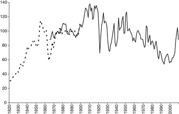
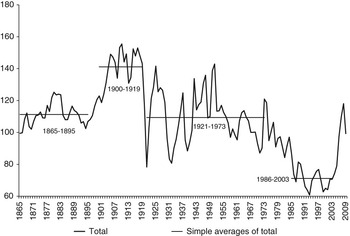
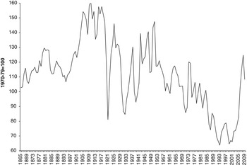
As in other studies, and despite the differences between the series caused by the varying weightings of products’ shares in total world export and the series’ cyclical variability, a marked long-term downturn is clearly seen. For the period 1862-1999, for example, Cashin and McDermott (Reference Cashin and McDermott2002) found a downward trend of 1.3 per cent per year, using The Economist’s industrial commodity price series and the U. S. GDP as a deflatorFootnote 10. Indeed, this is a first major conclusion of our analysis. The cumulative decline of the commodity terms of trade over the 20th century is very large: 53 per cent between the average of first two decades of the 20th century (when, as Figure 1 indicates, they peaked) and 1998-2003 (i.e. during the years of the late 20th century financial crisis in emerging markets, when they bottomed out), falling at a rate of slightly under 1 per cent per year.
TOTAL REAL NON-FUEL COMMODITY PRICES, 1820-2009 (1890 = 100)
Sources: The doted line is estimated as the ratio of British wholesale prices from Mitchell (Reference Mitchell1973, pp. 815-819) and the export prices of textiles estimated from the U. K. and French trade statistics by Ocampo (Reference Ocampo1984, Table 3.4). The solid line comes from the sources described in Appendix A. We used 1890 = 100 to be able to have both series with the same base year. The number for 2009 includes data until October.

This downturn is a hallmark of the 20 thcentury, not the 19th century. In fact, in keeping with recent observations of Hadaas and Williamson (Reference Hadaas and Williamson2003) and Williamson (Reference Williamson2006), the series actually point to an improvement in real raw material prices in the late 19th and early 20th centuriesFootnote 11. The improvement was even more marked in the first half of the 19th century, if we compare the evolution of commodity prices with those of textiles, the main manufacture imported by developing countries at the time (see Figure 1). Furthermore, as Hadaas and Williamson pointed out, the sharp reduction in shipping costs that occurred in the 19th century benefited all countries, thus facilitating a possible simultaneous improvement in the terms of trade of all countries estimated as the ratio of f.o.b. export prices to cost insurance and freight (c.i.f.) import pricesFootnote 12.
The decline of commodity prices in the 20th century was not continuous. Instead, it occurred in stepwise shifts that appear to have permanently altered price levels. Figure 2 graphs the total index, highlighting what appear to be these shifts. It is noteworthy that the largest price drops followed, with a lag, the two major slowdowns in the industrialized economies’ long-term growth rates during the First World War and in 1973, respectively (see Maddison Reference Maddison1995). This reflects the crucial role that the world economic growth has as a determinant of the commodity terms of trade, a point that comes out in the structural literature mentioned in the last paragraph of the previous section.
TOTAL REAL NON-FUEL COMMODITY PRICE INDEX, 1865-2009 (1970-1979 = 100)
Sources: For this and the following figures, see Appendix A. The number for 2009 includes data until October. Straight lines are simple averages for the corresponding periods.

In contrast to these downward shifts, there was an upward shift in the commodity terms of trade in the early 20th century, which continued through the First World War and the post-war boom. It may have started earlier. There might also have been an upward shift during the boom of the early 21st century (2004 to the first half of 2008). However, although this was the most impressive commodity boom in a century, in terms of length, coverage and intensity (World Bank 2009), it is too early to tell whether it was the beginning of a long-term change (i.e. a structural break in the series). The commodity price collapse experienced during the world economic crisis that erupted in late 2008 raises some doubts in this regard; still, the estimated 2009 level (with data until October) included in Figures 1 and 2 indicates that the commodity prices are currently high when compared with those that were characteristic during the last two decades of the late 20th century and early years of the 21st century.
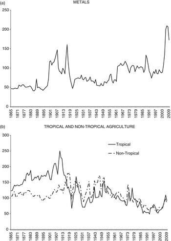
Trends and shifts have not been uniform by commodity groups. As Figure 3 highlights, the decline in terms of trade seems to be limited to agricultural products and not to metals. Rather, the latter (panel a) shows a fairly flat trend and sharp increases during the two major booms of the early 20th and early 21st centuries, indeed reaching in recent years the highest real values of the century and a half covered by our analysis. In turn in panel b, which shows a comparison between (mainly) tropical and (mainly) non-tropical agriculture, it is evident that the worst long-term decline was that experienced by tropical agriculture, as reflected in the strength of the two major downward shifts of the 20th century. Non-tropical agriculture lies in between, sharing in particular the downward trend through the 20th century.
TERMS OF TRADE BY COMMODITY GROUPS (1970-1979 = 100).

These observations suggest that, rather than discussing whether or not there was a secular downtrend in the barter terms of trade for commodities over the 20th century, it would be more appropriate to talk about the particular dynamics exhibited by this decline and how the evolution of different commodity groups coincided or diverged from the average pattern. The P–S hypothesis has traditionally — and perhaps erroneouslyFootnote 13 — been associated with a secular or continuous trend. This study considers the hypothesis that this deterioration took place in a stepwise fashion and mainly affected agricultural products.
The following analysis deals with the dynamics of each series. While it is clear that during the 20th century most commodities’ purchasing power dropped significantly, neither the size of this cumulative decrease nor the average annual growth rates provide a basis from which to infer the series’ long-term growth behaviorFootnote 14. In order to understand their behavior, it is necessary to know how the series respond to shocks and, in particular, whether or not they exhibit a stochastic component. Along with recent literatureFootnote 15, in the analysis we are particularly interested in evaluating possible structural breaks in the series.
4 COMMODITY PRICE DYNAMICS
4.1 Autoregresive Dynamics of the Series
As described in Ocampo and Parra (Reference Ocampo and Parra2003), two types of autoregressive processes may give rise to statistical trends that display different dynamicsFootnote 16. A deterministic trend (DT) model, if the series are stationary in variance, exhibits the following dynamics: Log Pt = βTt + ARMA(p,q)et, where Tt is a trend variable, et is an i.i.d. (independent and identically distributed) random shock and the parameter β is the trend (exponential growth rate), which can be estimated using traditional econometric procedures (ordinary least squares)Footnote 17. The only information required in this model to forecast the long-term price trend is the average growth rate of the variable (β), since shocks are transitory and thus do not affect the long-term projections.
In turn, a stochastic or stationary trend (ST) model, in the case of series exhibiting non-stationarity in variance, exhibits the following dynamics: ΔLog Pt = γ + ARMA(p, q) μt, where Δ is the first difference operator and γ is the average growth rate of the variable. The presence of μt Footnote 18, an i.i.d. random variable, will induce stochastic behavior in price levels. This model would be appropriate if the series is found to have a unit root. Consequently, in addition to a possible DT (γ), in this case shocks can have permanent effects on commodity price levels. If γ is statistically significant, then we have a unit root process with drift. For example, Cuddington et al. (Reference Cuddington, Ludema and Jayasuriya2002) show that if the price index is found to be following a DT process, then the trend can be regarded as significant (on the order of −0.3 per cent per year). If, on the other hand, it is found that it follows an ST process, then, given the high variance of the series in differences, the null hypothesis of a zero growth rate cannot be rejected.
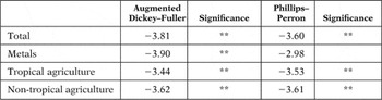
In Table 1, we test the four indices using both Augmented Dickey-Fuller (ADF) and non-parametric Phillips-Perron (PP) unit root tests. As can be observed, according to the ADF tests, the null hypothesis for non-stationarity (existence of a unit root) cannot be discarded for any of them. Using the PP test, the same hypothesis can be discarded only for metal prices.
UNIT ROOT TESTS FOR THE LOGARITHM OF THE SERIES IN REAL TERMS, 1865-2009

Source: Authors’ estimations. The Schwarz Info Criterion was used to determine the number of lags for the Augmented Dickey–Fuller. The Newey–West bandwidth automatic selection criterion was used for the Phillips–Perron test.
*, **, ***: 99%, 95% and 90%, respectively, in the event that the null hypothesis of a unit root can be rejected. For example, * would mean that at 10% significance, a unit root can be rejected.
The literature indicates that these two tests tend to lead to a false non-rejection of the null hypothesis of a unit root, especially if the series has structural breaksFootnote 19. What is more, if very small samples are being used and the shocks dissipate slowly, there may be very few independent observations of the process and, in that context, the estimation of DT models may generate more reliable parameterizations of the data (León and Soto Reference León and Soto1995b). In the case of primary commodity prices, evidence has been found that suggests the existence of structural breaks or instability in the parametersFootnote 20. In this instance, the sample is finite and the speed at which the shocks dissipate is unknown.
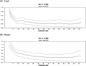
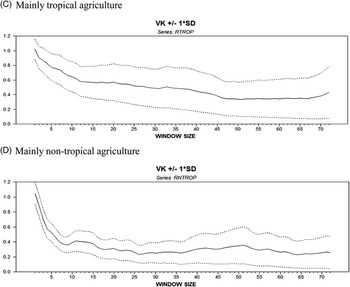
We use León and Soto (Reference León and Soto1995a and Reference León and Soto1995b) recursive estimation procedures to determine the ratio between the variance of innovation and the variance of the series. This estimator (Vk) makes it possible to see, from period to period (recursively), whether a shock changes the series’ variability temporarily or permanentlyFootnote 21. If a series Yt follows a DT process, then no innovation has a permanent effect (i.e. the permanent component is null). Thus, in the long run, the variance of innovations and the Vk estimator will trend toward zero. If Yt is a random walk, then innovation is wholly captured by the permanent component, so the variance of innovations will tend to equal the variance of the series, and the variance ratio will be one. In an intermediate process such as the ST process, Vk will be between zero and one. The Vk estimator also makes it possible to describe the response of the barter terms of trade based on a characteristic dissipation pattern (see section 4.3).
The results of this estimation are presented in Figure B1 in Appendix BFootnote 22. The thick lines depict the trend of the Vk estimator from period to period. The dotted lines trace its 95 per cent confidence interval. If, throughout the period, Vk (or its confidence interval) trends toward one, then the series exhibits a high level of persistence and therefore is not stationaryFootnote 23. In relation to our indices, the null hypothesis for Vk trending toward one can be rejected and it can thus be concluded that they do not exhibit non-stationarity. Although the analysis conducted up to this point would lead us to believe that a DT model should be used for the indices, our basic hypothesis is that the deterioration occurred in a stepwise fashion, which would point to the presence of structural breaks in the seriesFootnote 24. This question will be explored in the following section.
4.2 Structural Breaks
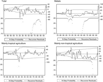
The first step in this direction is to analyze the possible presence of structural breaks in series that probably follow the deterministic-trend modelFootnote 25. Following Cuddington et al. (Reference Cuddington, Ludema and Jayasuriya2002), we calculate first the recursive residuals and the error bands for the hypothesis that the residuals come from the same distribution as those from the estimated model. We also show probabilities (P-values) for an N-step forecast test for each possible sampleFootnote 26. The results appear in Figure 4. As can be seen, these tests suggest the presence of possible structural breaks around the 1890s, 1910s-1920s and in the 1970s-1980s.
RECURSIVE RESIDUALS TEST FOR STRUCTURAL BREAKS
Source: Eviews graph estimates based on authors’ data.

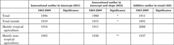
In Ocampo and Parra (Reference Ocampo and Parra2003), we used Perron’s test (Reference Perron1997) to select a break point that minimized the t-statistic for testing the null hypothesis of a unit root. In Table 2, we present the results for our four indices. We test whether the structural break is only in the IO1 (innovational outlier in intercept) or AO (additive outlier in trend), or in both (IO2). As the results indicate, the latter is the most interesting case.
PERRON’S TEST FOR ENDOGENOUS DETERMINATION OF DATE OF A STRUCTURAL BREAK VS. NULL HYPOTHESIS OF UNIT ROOT

Source: Authors’ estimations.
Note: *, **, ***: 99%, 95% and 90% significance, respectively.
The null hypothesis of a unit root can be rejected with a 95 per cent confidence level with respect to the alternative hypothesis of a structural break for non-tropical agriculture and with a 90 per cent confidence level for all the rest but tropical agriculture, using the IO2 model. It is clear, however, that the presence of a structural break does not preclude the possible presence of one or more additional breaks.
Cuddington et al. (2002) put forward that this is a test whose null hypothesis is the presence of a unit root, conditional on the possible presence of a structural break at an unknown date, and not a test for the presence of a structural break. They point out that it allows for only one structural break, whereas there is a priori no reason to believe that additional breaks may not be present. They also identify the fact that the test allows for the structural break under the alternative hypothesis but not under the null hypothesis as a weakness. Lastly, the test assumes that the type of structural break is known a priori. That is why we run the test for the three models, without assuming that we know beforehand which one is most appropriate.
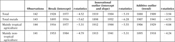
Kellard and Wohar (Reference Kellard and Wohar2006) use a test developed by Lumsdaine and Papell (Reference Lumsdaine and Papell1997) that allows for the possibility of two endogenous break points. We use this method, as adapted for WinRATSFootnote 27 to evaluate the presence of more than one structural break. The procedure allows for the presence of breaks in the intercept, the trend or both. We present the results in Table 3.
LUMSDAINE AND PAPELL’S TEST FOR ENDOGENOUS DETERMINATION OF THE DATE OF MORE THAN ONE STRUCTURAL BREAK VS. NULL HYPOTHESIS OF UNIT ROOT

Source: Authors’ estimations.
These estimates indicate again that the largest changes in commodity price trends were concentrated sometimes in the 1890s, the 1910s and 1980s. Some explanations of the first of these breaks could be the change in the world price trends from deflation to inflation, which took place after 1897, and the particular demands generated by the technological revolutions of the late 19th century (automobile and electricity). The second and third breaks most likely represent the delayed effects of the sharp slowdowns in the world economy after the First World War and after the first oil shock of the 1970s (Maddison Reference Maddison1995), respectively. More precisely, the second of these breaks can be associated with the severe deflationary crisis that took place in 1920-1921 after the First World War, whose effect on raw materials’ prices is well known, whereas the third can be linked with the monetary shock generated by the actions of the U. S. Fed in 1979 to curb inflation and which led to the debt crisis in Latin America and other parts of the developing worldFootnote 28.
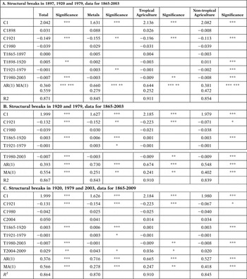
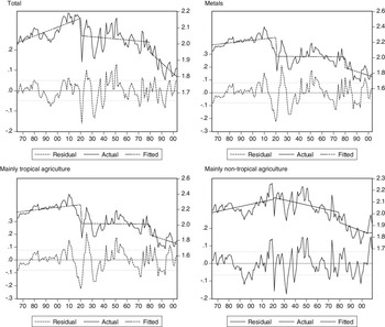
The econometric exercises reported in Table 4 therefore assume that the structural breaks took place in 1897, 1920 and 1979. In the first case, the break does not seem to capture the dynamics of the series, particularly of mineral prices, which is one of the most interesting in the late 19th and early 20th century, and hence, in the analysis given below, we prefer the second set of regressions, which assumes no structural break in 1897. The two structural breaks coincide, therefore, with those of Table 3 for the total commodity price index with the IO2 model. However, regression exercises indicated that, for more recent decades, a break in 1979 turns out to better capture the dynamics of the price series than one in the mid-1980s. In addition, since, compared to previous results from Ocampo and Parra (Reference Ocampo and Parra2003), adding the data for recent years significantly affects the post-1979 trends, we estimated the model with data up to 2003 (the end of the emerging market crisis of the late 20th century) and for the full sample, but adding a new hypothetical structural break in the early 21st century (in 2003). Figure 5 shows the results for the second set of regressions reported in Table 4 (breaks in 1920 and 1979, with data for 1865-2003); in the Figure, we exclude the ARMA dynamic of the residuals included in the econometric analysis to illustrate more clearly the breaks and the deviations of prices from the estimated trends.
REGRESSION ESTIMATIONS WITH STRUCTURAL BREAKS

Source: Authors’ estimations.
Note: *, **, ***: 99%, 95% and 90% significance, respectively.
ESTIMATION OF TRENDS IN PRICE INDICES WITH STRUCTURAL BREAKS. IN 1920 AND 1979, DATA FOR 1865-2003
Source: Eviews graph estimates based on authors’ data.

These exercises show that there was an upward trend of commodity prices of 0.3 per cent per year in 1865-1920. This was associated with trends in both metals and non-tropical agriculture; in the case of metals, the upward trend was actually double the average for non-fuel commodities (0.6 per cent per year). In contrast, tropical agriculture did not experience an upward trend.
In 1920, all indices experienced a strong and sudden decline, from which they failed to recover in subsequent decades. The decline is statistically significant, though of varying magnitude: between 7 and 22 per cent according to the second set of regressions, with the strongest shock being that experienced by tropical agriculture. Interestingly, this drop was followed by a long period (1921-1979) during which the agricultural price indices followed no statistically significant trend. This occurred because individual prices moved in opposite directions. In contrast to the trends in agriculture, mineral prices did experience a small and weakly significant upward trend that by the end of the period the prices had more or less reversed the sharp reduction that had taken place around 1920; Figure 5 indicates that the upward trend of mineral prices was noticeable only after the Second World War.
Finally, in contrast to what had happened in 1920, in the late 1970s, there was no sudden drop in prices, but rather a break in the price trend for the overall index and agricultural prices, which became strongly negative from then on. For these indices, the rate of decline was of 0.9 per cent a year. The trend for metals was also negative but not statistically significant. A closer analysis might indicate that the decline was concentrated in the 1980s (see Maizels Reference Maizels1992, for an analysis of changes in raw materials’ prices in that decade), in which case this phenomenon would be more similar to what took place in 1920, though it was more gradual over time. In any case, these results are less adverse than those estimated by Ocampo and Parra (Reference Ocampo and Parra2003), indicating that the new commodities that were added into the basket on top of those included by G-Y, performed better than more traditional commodities.
Finally, if we introduce a 2003 structural break, the major change is a positive trend in the price of metals and tropical agriculture, though the significance of the coefficients estimated for these two subindices is statistically weak. As already pointed out, the short period that has elapsed makes it impossible to identify whether it is really a long-term break.
The statistical exercises therefore seem to indicate that there was a small upward trend of commodity prices since the mid-19th century that lasted until the First World War. This was followed by a strong reduction in real commodity prices throughout the rest of the 20th century, which can be explained by two major structural breaks that took place around 1920 and 1979. The first of these breaks took the form of a sudden, one-time drop in prices, and the second took the form of a shift in the trend of commodity prices. Tropical agriculture did not enjoy the improvement in commodity prices of the late 19th and early 20th centuries and the commodity group was most affected by adverse shocks, particularly that of 1920. In contrast, mineral prices performed better: the early boom was stronger, the 1921-drop was gradually reversed in the following decades and there was no statistically significant drift in the late 20th century.
To complete this overview, the following section contains a brief analysis of the series’ speed of mean reversion in response to short-term shocks. A slow speed of mean reversion would imply that short-term shocks have a long-lasting effect on economic performance.
4.3 Variability and short-term shocks
The VK estimator, which was used to determine the long-term persistence of innovations, is also useful for analyzing the series’ reaction to short- and medium-term shocks without resorting to methodologies based on parameterizations that give too much weight to short-term movements. The speed with which the estimator tends toward zero shows how a shock is dissipated. Following the methodology of León and Soto (Reference León and Soto1995b), Table 5 illustrates the behavior of this estimator.
ESTIMATIoN OF THE MEAN REVERSION PROCESS (VALUE OF THE VK STATISTIC)

Source: Authors’ calculations.
This analysis reveals that of the three subindices, only that for non-tropical agriculture shows a fair speed of mean reversion (VK < 0.75 after 5 years), but price shocks in markets for metals and tropical agriculture show strong persistence; the overall index shows an intermediate outcome. After this initial reversion, the process continues at a slower pace, so that only the non-tropical agriculture price index returned to long-term equilibrium (VK < 0.26) after more than 25 years. Viewed from a macroeconomic standpoint, these results show that, despite the relative speed of mean reversion, the effects of a shock last for several years, and therefore have an impact in both the short and medium terms. An interesting implication is that, although stabilization funds are a viable option, the reference prices used by such funds must change according to market prices to prevent large-scale fiscal losses associated with their management.
5 Conclusions
The econometric results presented in this paper indicate that commodity prices experienced a major break in its long-term trend in the aftermath of the First World War. The positive trend that had characterized metals and non-tropical agriculture commodity prices in the late 19th and early 20th centuries, though not those for tropical agricultural products, was followed by a strong long-term decline, which took place in a stepwise rather than a secular way, with the major structural breaks taking place after the two major slowdowns of the world economy.
The first downward shift happened around 1920 and was related to the major global economic changes produced by the First World War. The second structural break seems to have occurred around 1979, in the wake of the world economic slowdown that began in 1973 and the policies adopted to stop rising inflation in the industrial world. Whereas the first involved a large one-time generalized downward adjustment of commodity prices, the second led to an adverse shift in price trends for agricultural, though not for mineral, commodities. Over the long-term, the decline was quite substantial: overall commodity prices more than halved between the average of the first two decades of the 20th century and the average for 1998-2003. Tropical agriculture experienced the strongest decline and metals the weakest one — indeed, perhaps no significant long-term decline. The first decade of the 21st century may have seen a positive structural break in commodity prices, but it is too soon to tell.
One interesting implication is the central role played by world economic growth in the determination of the two major breaks experienced over the 20th century (and, perhaps, in the opposite direction, in the late 19th and early 21st centuries). Hence, the effect of long-term world economic growth on the demand for commodities seems to be a crucial determinant of commodity price trends, as emphasized by the first variant of the P–S hypothesis and structural models of commodity price formation. Nonetheless, the asymmetric adjustment of prices and incomes during crises emphasized by the second variant of the P–S hypothesis may be part of the explanation. The absence of a positive trend of tropical agricultural prices before the First World War and its stronger long-term downward trend through the 20th century is also consistent with the second version of the hypothesis.
Viewed in temporal terms, except for these trends in tropical agriculture, pre-Second World War trends are hard to explain in terms of center–periphery income divergence. Rather, the upward trend of commodity prices up to the First World War was an opportunity that several developing countries, particularly in Latin America, exploited. The timing of the major trends after the Second World War is more consistent with the second version of the P–S hypothesis: up to the 1970s, there was a slow or no divergence of incomes between developed and developing countries, and commodity prices showed no trend; in contrast, the quarter century after 1979 was both a period of a sharp increasing divergence between commodity-producing regions in the developing world and the center of the world economy, and of plunging agricultural prices.
As little long-term information is available on productivity and changes in product quality comparable to the price series examined above, it is difficult to include these variables in the statistical exercises. In any event, existing series for the OECD countries indicates that while manufacturing productivity rose faster than agricultural productivity up to around 1950, the opposite has been the case since then (Bairoch Reference Bairoch1989; Maddison Reference Maddison1991). This structural break is not, however, reflected in the foregoing statistical results. Furthermore, the long-term lead gained by agricultural productivity, as revealed by these data, would only explain a relatively marginal decline in agricultural terms of trade (of about 0.2 per cent a year).
Series on productivity per hectare for seven agricultural products, estimated by Scandizzo and Diakosawas (Reference Scandizzo and Diakosawas1987) and updated with information from the Food and Agriculture Organization of the United Nations indicate annual productivity improvements of around 1 per cent throughout the 20th century, with the notable exception of coffee, for which productivity increased by just 0.2 per cent a year between 1910-1914 and 1995-1999. The rate of productivity growth sped up between the 1960s and the 1980s for three products that were affected by the «green revolution» (rice, maize and wheat). The inclusion of these productivity series in the statistical exercises does not, however, change the conclusions to be drawn concerning the long-term real price trends; in fact, their impact on real prices seems to have been only partial and not always statistically significant.
The negative trend experienced by the commodity prices through the 20th century is consistent with the results of Ocampo and Parra (Reference Ocampo and Parra2003) for individual products: four commodities showed a positive trend; eleven showed no trend or drift, with five of them experiencing a cumulative decline of nearly 60 per cent, indicating the predominance of negative shocks; and nine showed a negative trend.
Finally, the economic and historical literature is rich with analysis of the broader issue of the relation between the commodity price trends with industrialization and deindustrialization in the periphery (see, in particular, Williamson Reference Williamson2006, and our own reflections in Ocampo and Parra Reference Ocampo and Parra2006 and Reference Ocampo and Parra2007). However, this rich debate unleashed by the P–S hypothesis is beyond the scope of this paper.
Appendix A: Methodology used to extend and update the commodity price indices
Data for 1865-1900 was kindly provided by professor Jeffrey Williamson (Blattman et al. Reference Blattman, Hwang and Williamson2004). Its main source was various issues of the Journal of the Royal Statistical Society, where Mr Sauerbeck’s well-known commodity price statistics were published initially and then updated.
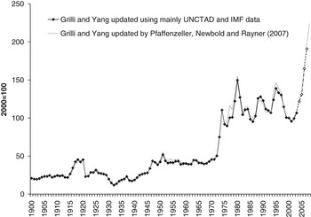
Ocampo and Parra (Reference Ocampo and Parra2003) used UNCTAD and IMF commodity prices to update the G-Y series until 2000. Pfaffenzeller et al. (Reference Pfaffenzeller, Newbold and Rayner2007) published the actual list of the product used by Grilli and Yang and a detailed update until 2003. These authors went back to the original series used by Grilli and Yang and recalculated them since 1900, resulting in slight differences with respect to the original series. Since we do not have access to some historical series from the World Bank used by these authors and the differences are not particularly significant (see Figure A1), we use our own estimates.
COMPARISON BETWEEN GRILLI AND YANG’S UPDATES OF TWENTY-FOUR COMMODITY PRICES
Sources: Grilli and Yang (Reference Grilli and Yang1988) and authors’ calculations based on prices as described in Table A1 and other sources as described in this Appendix. Pfaffenzeller et al. (2007) updated the series until 2003. Data until 2007 was kindly made available by Mr Pfaffenzeller and can be found at http://www.stephan-pfaffenzeller.com/cpi.html.

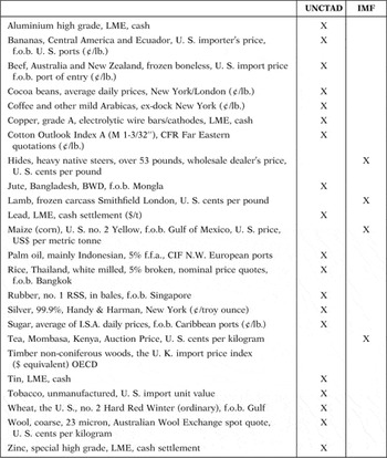
In this paper, we continue to use the original G-Y historical series and mainly UNCTAD and IMF prices when extending the series until 2009. Table A1 shows the exact description of the products included.
SPECIFIC PRICES INCLUDED IN THE COMMODITY PRICE INDICES

Notes: LME: London Metal Exchange, CFR: Code of Federal Regulations, BWD: Bangladesh White D, FFA: Free Fatty Acid, NW: North Western, ISA: International Sugar Agreement.
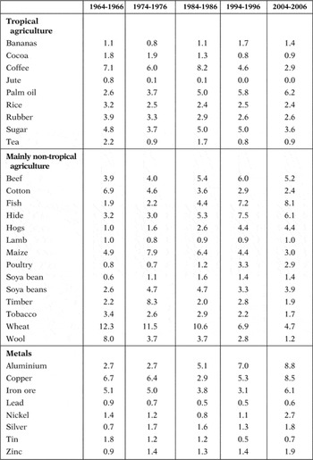
Ocampo and Parra (Reference Ocampo and Parra2003) used weightings for the share of world exports represented by each commodity in 1977-1979, as developed by Grilli and Yang (Reference Grilli and Yang1988)Footnote 29. Using the UN-Comtrade data, we calculated the weights of thirty-one commodities since 1964-1966. The results for selected years are presented in Table A2. These weights are used until 1969. After that year, the weights for 1984-1986 are used. A prior analysis indicated that the new weights captured an intermediate result from those using the alternative ones offered by Table A2.
EVOLUTION OF THE SHARE OF PRIMARY COMMODITIES IN THE WORLD TRADE SINCE 1964-1966

Source: Authors’ calculations, based on the UN-Comtrade, using SITC-1, instead of SITC-2 to be able to include data before 1976.
In Figure A2, we present the evolution of the commodity prices including gold, a major commodity usually left aside in these exercises. As gold exports are not included in the UN-Comtrade, we cannot calculate its weight directly in Table A2. Instead, we calculate its weight using the world production valueFootnote 30. However, since the price of gold is strongly associated with its monetary use (including as central banks’ reserves) and was a regulated price until 1971, it does not follow the fundamental determinants of the commodity terms of trade in general. Hence, finally, we decided to exclude this commodity from our analysis. In any case, as Figure A2 shows, the basic trends remain after we include the gold into the price series.
INDEX OF COMMODITY PRICES INCLUDING GOLD

Appendix B
RECURSIVE Vk ESTIMATES OF SHOCK PERSISTENCE (VERTICAL AXIS: Vk; HORIZONTAL AXIS: TIME)
Continued

(Continued).