


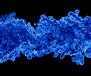

1. Introduction
Strong turbulent transport of passive scalars is among the most important beneficial effects of turbulence, with obvious consequences for the dispersion of emitted pollutants and the efficiency of combustion and other chemical reactions. There is a vast literature on various aspects of turbulent diffusion, transport and mixing of scalar fields and their application to diverse engineering and environmental problems. Perhaps the significance of heat transfer and passive scalars in turbulent flows was realized through an early wind-tunnel experiment in an axially symmetric heated-air jet by Corrsin (Reference Corrsin1943). Thereafter, an impressive amount of work has been devoted to the study of scalar fields in various turbulent flows (e.g. Corrsin & Uberoi Reference Corrsin and Uberoi1950; Wilson & Danckwerts Reference Wilson and Danckwerts1964; Townsend Reference Townsend1976; Warhaft & Lumley Reference Warhaft and Lumley1978; Tavoularis & Corrsin Reference Tavoularis and Corrsin1981; Dahm & Dimotakis Reference Dahm and Dimotakis1990; Dowling & Dimotakis Reference Dowling and Dimotakis1990; George Reference George1992b; Mydlarski & Warhaft Reference Mydlarski and Warhaft1998; Warhaft Reference Warhaft2000; Lubbers, Brethouwer & Boersma Reference Lubbers, Brethouwer and Boersma2001; Hearst et al. Reference Hearst, Buxton, Ganapathisubramani and Lavoie2012; Bahri et al. Reference Bahri, Arwatz, George, Mueller and Hultmark2015; Sreenivasan Reference Sreenivasan2019).
The interaction between the velocity and passive scalar (temperature) fields, among other things, has been of great interest to the turbulence community. To study the influence of the turbulent velocity field on the passive scalar field, a combination of the transport equations for both the scalar and velocity fields is required to be considered. This study has been closely connected to a variety of theoretical approaches to model the terms in the transport equations, as early as the 1900s, when Prandtl proposed the eddy diffusivity concept.
From a theoretical point of view, the mixing of the velocity and scalar fields has been notably treated in terms of self-similarity theory. In the context of turbulence, one of the great theoretical efforts has been to identify the relevant scaling parameters based on self-similarity analysis with the aid of experimental and numerical data that enable scientists to model turbulence quantities in flows that are experienced in real life. The traditional concept of self-similarity, or self-preservation, which assumes that the flow scales with single turbulent parameters, has been extensively used to describe the spatial and temporal evolution of turbulence quantities. It is known that the classical scaling parameters (based on a self-preservation analysis) for turbulent shear flows were identified by Townsend (Reference Townsend1956, Reference Townsend1976). He also proposed the idea of a ‘universal’ self-similar solution, which indicates that such a solution is unique and independent of initial and boundary conditions.
The turbulent jet is arguably known as one of the most intensely studied turbulent flows, which has attracted a substantial amount of attention in terms of self-similarity analysis. This is mainly because of its relevance to a plethora of applications such as combustion, chemical processes, pollutant discharge and cooling, mixing and drying processes. Not only the velocity field, but also the turbulent jet flow has been widely studied for its mixing scalar properties using self-similarity analysis as can be found in various articles such as Gouldin et al. (Reference Gouldin, Schefer, Johnson and Kollmann1986), Dahm & Dimotakis (Reference Dahm and Dimotakis1990), Dowling & Dimotakis (Reference Dowling and Dimotakis1990), Lubbers et al. (Reference Lubbers, Brethouwer and Boersma2001), Mi, Nobes & Nathan (Reference Mi, Nobes and Nathan2001), Burattini & Djenidi (Reference Burattini and Djenidi2004), Carazzo, Kaminski & Tait (Reference Carazzo, Kaminski and Tait2006), Darisse, Lemay & Benaïssa (Reference Darisse, Lemay and Benaïssa2005) and Darisse, Lemay & Benaïssa (Reference Darisse, Lemay and Benaïssa2013).
According to the classical self-similarity (e.g. Townsend's) approach, the equations governing the evolution of the mean scalar field, turbulent scalar flux and scalar variance in a turbulent jet satisfy similarity if the following hold (Dahm & Dimotakis Reference Dahm and Dimotakis1990):
 $$\begin{gather} \bar \varTheta = \varTheta_{s}(t) f_{\theta} (x_2/L_{\theta}), \end{gather}$$
 $$\begin{gather}R_{i\theta}^0 = U_s(t) \varTheta_{s}(t) g_{i\theta} (x_2/L_{\theta}) \end{gather}$$
and
 \begin{equation} R_{\theta \theta}^0 = \varTheta_{s}(t)^2 g_{\theta\theta} (x_2/L_{\theta}), \end{equation}
where  $\bar \varTheta$ is the mean scalar field,
 $R_{i\theta }^0$ (
 $= \overline {u_i\theta }$) is the turbulent scalar flux and
 $R_{\theta \theta }^0$ (
 $=\overline {\theta ^2}$) is the scalar variance (here,
 $x_2$ represents the cross-stream direction and
 $t$ is time). Note that we denote the one-point scalar quantities with the superscript ‘
 $0$’ throughout this paper in order to clearly distinguish them from the corresponding two-point double correlation functions. Further,
 $\varTheta _{s}$ is a scalar scale,
 $U_s$ is a velocity scale and
 $L_{\theta }$ is a (scalar) length scale, which may all depend on time. In (1.1)–(1.3),
 $f_{\theta }$,
 $g_{i\theta }$ and
 $g_{\theta \theta }$ are the dimensionless self-similar functions, which depend on
 $x_2$, which is scaled by
 $L_{\theta }$, that may also depend on time.
While the similarity of the mean profile has been well supported by experimental and numerical data (Dahm & Dimotakis Reference Dahm and Dimotakis1990; Darisse et al. Reference Darisse, Lemay and Benaïssa2005, Reference Darisse, Lemay and Benaïssa2013), there has been substantial scatter between the results of different investigations in terms of the self-similarity of the turbulent scalar flux and the scalar variance in the turbulent jet (Lockwood & Moneib Reference Lockwood and Moneib1980; Dahm & Dimotakis Reference Dahm and Dimotakis1990; Dowling & Dimotakis Reference Dowling and Dimotakis1990; Lubbers et al. Reference Lubbers, Brethouwer and Boersma2001). For example, through conducting a numerical study, Lubbers et al. (Reference Lubbers, Brethouwer and Boersma2001) noted that the mean scalar profiles are self-similar in agreement with the classical similarity analysis; however, the variance of the scalar fluctuations is found to be not self-similar. They commented that this observation is in contrast with the results of Dowling & Dimotakis (Reference Dowling and Dimotakis1990) who claimed that this variance is also self-similar. Lubbers et al. (Reference Lubbers, Brethouwer and Boersma2001) concluded that the self-similarity is unlikely from a theoretical point of view.
In order to contrast it with the new scaling in § 3, here we also examined the classical scaling of the turbulent flux  $R_{i\theta }^0$ and scalar variance
 $R_{\theta \theta }^0$ by using (1.2) and (1.3), and a new set of direct numerical simulation (DNS) data, which are plotted in figure 1. Additionally, the mean scalar field
 $\bar \varTheta$ scaled using (1.1) is included in figure 1. As widely used in the literature,
 $\varTheta _{s}$ was chosen to be the maximum magnitude of the mean scalar
 $\bar {\varTheta }$ on the centreline (
 $\bar {\varTheta }_c$), and
 $L_{\theta }$ was selected to be the mean scalar half-width
 $\delta _{\theta }$ defined as the distance between the location along
 $x_2$ at which the mean scalar is equal to half of the maximum mean scalar and the centreline. As expected, the self-similarity of the mean scalar field is satisfactory. However, for the second moments, only the profiles of the turbulent scalar flux
 $R_{2\theta }^0$ show a good collapse for different
 $t$ whereas the turbulent scalar flux
 $R_{1\theta }^0$ and scalar variance
 $R_{\theta \theta }^0$ obviously depart from a full similarity. As discussed above, despite the fact that the classical self-similarity and scaling parameters for turbulent jets have been known for a long time, some significant deviation from the complete self-similarity of the second and higher moments of the scalar or velocity is observed when using the classical scalings (where an a priori set of similarity scales is used). This is clearly noted in the literature as well as a wide scatter in the results implies the strong need of investigating this problem using more advanced methods. Therefore, it is the main aim of this paper to use a more general technique based on Lie symmetry group analysis to formally derive the similarity of the first, second and third moments for the passive scalar quantities for a temporally evolving turbulent plane jet. A temporally evolving turbulent jet set-up is known to be a good compromise between our ability to use accurate numerical methods, the computational efforts for sufficiently large Reynolds number and capturing the physics of turbulent jets (e.g. da Silva & Pereira Reference da Silva and Pereira2008; van Reeuwijk & Holzner Reference van Reeuwijk and Holzner2013; Krug et al. Reference Krug, Holzner, Marusic and van Reeuwijk2017; Cimarelli et al. Reference Cimarelli, Mollicone, van Reeuwijk and De Angelis2020; Denker et al. Reference Denker, Attili, Boschung, Hennig, Gauding, Bode and Pitsch2020). Therefore, the combination of newly derived similarity solutions and DNS of temporal jets seems to represent a useful combination of tools for the analysis of the important features of turbulent jet flows.
The mean scalar field,  $\bar \varTheta$ (a), the turbulent scalar fluxes,
 $R_{1\theta }^0$ (b) and
 $R_{2\theta }^0$ (c), and the scalar variance,
 $R_{\theta \theta }^0$ (d), normalized by classical scaling parameters according to (1.1)–(1.3). The data are from the current DNS (DNS2), the details of which are provided in § 4.

Sophus Lie, in the nineteenth century, introduced symmetry analysis of a system of differential equations based on continuous transformation groups to unify and extend various specialized methods for solving differential equations, which has had a profound influence in various areas of mathematics and physics. What makes Lie symmetry a powerful method in relation to the turbulence problem is its capacity to unify and extend various specialized methods for solving complex differential equations. In simple language, when applying a symmetry transformation to equations, their formal structures remain unchanged. The Lie symmetry contains many profound concepts, a detailed description of which is available in several textbooks such as Hydon (Reference Hydon2000) and Bluman, Cheviakov & Anco (Reference Bluman, Cheviakov and Anco2010) and previous publications by the present authors (e.g. Oberlack Reference Oberlack2001; Oberlack et al. Reference Oberlack, Waclawczyk, Rosteck and Avsarkisov2015; Sadeghi, Oberlack & Gauding Reference Sadeghi, Oberlack and Gauding2018; Sadeghi & Oberlack Reference Sadeghi and Oberlack2020). Therefore, in this paper, we only briefly review a schematic of this method in Appendix A.
The application of Lie symmetry group theory in turbulence has been developed by Oberlack and co-authors over a time span of 20 years (e.g. Oberlack Reference Oberlack2001; Oberlack & Rosteck Reference Oberlack and Rosteck2010; Avsarkisov, Oberlack & Hoyas Reference Avsarkisov, Oberlack and Hoyas2014; Waclawczyk et al. Reference Waclawczyk, Staffolani, Oberlack, Rosteck, Wilczek and Friedrich2014; Oberlack et al. Reference Oberlack, Waclawczyk, Rosteck and Avsarkisov2015; Sadeghi et al. Reference Sadeghi, Oberlack and Gauding2018; Sadeghi & Oberlack Reference Sadeghi and Oberlack2020; Sadeghi, Oberlack & Gauding Reference Sadeghi, Oberlack and Gauding2020). For example, they have studied the turbulent channel, the velocity field of a temporally evolving jet, the isotropic homogeneous turbulence and some other canonical wall-bounded and shear flows using Lie symmetry theory by investigating the infinite series of two-point correlation (TPC) and multi-point correlation equations. The symmetry analysis of these equations together with the application of invariant surface condition have allowed them to derive a variety of classical and new scaling laws in turbulence as the exact solutions of symmetry-invariant type of TPC and multi-point correlation.
In this context, it should be mentioned that in addition to the classical symmetry theory, the so-called equivalence transformation is a methodological approach that is at least similar (e.g. Bluman et al. Reference Bluman, Cheviakov and Anco2010). Here, the unclosed terms are taken as free functions and, as with symmetries, the structure of the equation is preserved, but the unclosed terms can take a different form. Indeed, unclosed equations such as those in § 2 involve a greater number of equivalence transformations than symmetry transformations; however, they are then no longer inevitably consistent with the equations for the higher correlations. Against this background, in the present work we focus solely on symmetry transformations that are also consistent with all higher correlation equations.
In the present research, we employ the Lie symmetry method to the thermal energy and a new type of TPC equations of a temporally evolving turbulent plane jet, which are the fundamental basis to find scaling laws. This is the first study to apply the symmetry analysis of passive scalar transport in a turbulent jet flow. As a consequence of the current analytical work, we propose new scaling laws (self-similar solutions) for the scalar quantities. The results of DNS are used to validate the new scaling laws.
This paper is organized as follows. The governing equations required for the symmetry analysis of a temporally evolving plane jet are given in § 2. In § 3, we present the theoretical (Lie symmetry) analysis of the governing equations for the current flow and derive new scaling laws. The DNS details and verification of scaling laws are presented in § 4. Finally, a summary is presented and conclusions drawn in § 5.
2. Governing equations
The first equation of interest is derived after employing the Reynolds decomposition  $U_i=\bar {U}_i+u_i$ and
 $\varTheta = \bar {\varTheta }+\varTheta$ into the transport equation for the (instantaneous) passive scalar
 \begin{equation} \frac{\partial \varTheta}{\partial t}+U_k\frac{\partial \varTheta}{\partial x_k} = \alpha \frac{\partial^2 \varTheta}{\partial x_k \partial x_k}, \end{equation}
followed by applying an ensemble averaging to obtain its averaged version, namely a transport equation of the mean scalar, i.e.
 \begin{equation} \frac{\partial \bar{\varTheta}}{\partial t}+\bar{U}_k \frac{\partial \bar{\varTheta}}{\partial x_k}={-}\frac{\partial R_{k\theta}^0 }{\partial x_k}+ \alpha \frac{\partial^2 \bar{\varTheta}}{\partial x_k \partial x_k}, \end{equation}
where  $\theta$ and
 $u_k$ are respectively the fluctuating parts of the scalar and velocity fields. Here,
 $\bar {\varTheta }$ is the mean scalar and
 $\bar {U}_k$ is the mean velocity (note that in this paper the overbar signifies the average). Additionally, the quantity
 $R_{k\theta }^0=\overline {u_k\theta }$ represents the effect of the turbulence in the transport of heat and it is commonly known as the turbulent heat flux vector. Recall that
 $\alpha$ is the thermal diffusion coefficient.
For a temporally evolving plane jet, where the flow is considered statistically homogeneous in the mean flow  $x_1$ and lateral
 $x_3$ directions and spreads in the inhomogeneous direction
 $x_2$ over time
 $t$, (2.2) reduces to
 \begin{equation} \frac{\partial \bar{\varTheta}}{\partial t} + \frac{\partial R_{2\theta}^0}{\partial x_2}- \alpha \frac{\partial^2 \bar{\varTheta}}{\partial x_2^2}=0. \end{equation}
By integrating (2.3) across the cross-stream direction ( $x_2$) and assuming both zero free stream turbulence and a vanishing gradient of
 $\bar {\varTheta }$ for
 $x_2 \to \pm \infty$, it is also confirmed that
 \begin{equation} I=\int_{-\infty}^{\infty} \bar{\varTheta}(x_2,t)\,\mbox{d}x_2 \end{equation}
is an integral invariant, i.e. a constant.
At this point, we present new forms of the equations for TPC, which are the main basis for the present analysis. As fully explained in Oberlack et al. (Reference Oberlack, Waclawczyk, Rosteck and Avsarkisov2015), Sadeghi et al. (Reference Sadeghi, Oberlack and Gauding2018) and Sadeghi & Oberlack (Reference Sadeghi and Oberlack2020), the concept of TPC has become an important analytical tool in turbulence for two main reasons. First, it delivers additional information on the turbulence statistics such as length scale. Second, in every higher-moment equation, only one additional unclosed function appears. Besides, a general symmetry analysis of the TPC equations has resulted in additional symmetries compared with only those that are implied by Navier–Stokes equations (Oberlack & Rosteck Reference Oberlack and Rosteck2010, Reference Oberlack and Rosteck2011; Avsarkisov et al. Reference Avsarkisov, Oberlack and Hoyas2014). These symmetries, which are denoted statistical symmetries, have been shown to play a key role in the understanding of the scaling laws in turbulent flows, especially for higher moments of the velocity. Traditionally, the dynamic equations for the TPC of the fluctuating parameters have been of interest to the turbulence community, mainly because of their straightforward relations to the one-point turbulent Reynolds stress or heat flux components. However, the nonlinear character of the TPC equations complicates further analysis concerning the symmetry (and similarity) analysis of them. To resolve this issue, we follow the idea in Oberlack & Rosteck (Reference Oberlack and Rosteck2010) to establish a novel set of two-point equations based on the instantaneous quantities (not the classical fluctuating quantities), which leads us to arrive at a set of linear equations. In the present work, we derive the equations for the TPC of the instantaneous velocity–scalar and instantaneous scalar–scalar functions, which in their most general forms respectively read (see detailed derivation steps in Appendix B)
 \begin{align} & \frac{\partial H_{i\varTheta}}{\partial t}+ \frac{\partial \overline{P\varTheta}}{\partial x_i}-\frac{\partial \overline{P\varTheta} }{\partial r_i}+ \frac{\partial H_{(ik)\varTheta}}{\partial x_k}-\frac{\partial H_{(ik)\varTheta}}{\partial r_k}+ \frac{\partial H_{i(\varTheta k)}}{\partial r_k} \nonumber\\ &\quad -\nu\left[ \frac{\partial^2 H_{i\varTheta}}{\partial x_k^2}-2 \frac{\partial^2 T_{i\varTheta}}{\partial x_k \partial r_k}+ \frac{\partial^2 H_{i\varTheta}}{\partial r_k \partial r_k} \right]-\alpha \left[\frac{\partial^2 H_{i\varTheta}}{\partial r_k \partial r_k} \right] = 0 \end{align}
and
 \begin{align} & \frac{\partial H_{\varTheta\varTheta}}{\partial t} +\frac{\partial H_{(\varTheta k)\varTheta}}{\partial x_k}- \frac{\partial H_{(\varTheta k)\varTheta}}{\partial r_k}+ \frac{\partial H_{\varTheta(\varTheta k)}}{\partial r_k} \nonumber\\ &\quad -\alpha\left[ \frac{\partial^2 H_{\varTheta\varTheta}}{\partial x_k^2}-2 \frac{\partial^2 H_{\varTheta\varTheta}}{\partial x_k \partial r_k}+2 \frac{\partial^2 H_{\varTheta\varTheta}}{\partial r_k \partial r_k} \right]= 0, \end{align}
where correlation vectors and tensors are defined as
 \begin{equation} \left.\begin{gathered} H_{i\varTheta}=\overline{U_i(\boldsymbol {x},t)\varTheta(\boldsymbol {x}+\boldsymbol {r},t)},\quad H_{\varTheta\varTheta}=\overline{\varTheta(\boldsymbol {x},t)\varTheta(\boldsymbol {x}+\boldsymbol {r},t)},\\ \overline{P\varTheta}=\overline{P(\boldsymbol {x},t)\varTheta(\boldsymbol {x}+\boldsymbol {r},t)}, \\ H_{(ik)\varTheta}=\overline{U_i(\boldsymbol {x},t)U_k(\boldsymbol {x},t)\varTheta(\boldsymbol {x}+\boldsymbol {r},t)}, \quad H_{(\varTheta k)\varTheta}=\overline{\varTheta(\boldsymbol {x},t)U_k(\boldsymbol {x},t)\varTheta(\boldsymbol {x}+\boldsymbol {r},t)}, \\ H_{i(\varTheta k)}=\overline{U_i(\boldsymbol {x},t)U_k(\boldsymbol {x}+\boldsymbol {r},t)\varTheta(\boldsymbol {x}+\boldsymbol {r},t)}, \\ H_{\varTheta(\varTheta k)}=\overline{\varTheta(\boldsymbol {x},t)U_k(\boldsymbol {x}+\boldsymbol {r},t)\varTheta(\boldsymbol {x}+\boldsymbol {r},t)}. \end{gathered}\right\} \end{equation}
Here,  $\boldsymbol {x}$ and
 $\boldsymbol {r}$ are coordinates in the physical and correlation spaces, respectively. We also define the function
 $H_{\varTheta \varTheta }^0$ as the limit
 $\boldsymbol {r} \rightarrow 0$ of the TPC function
 $H_{\varTheta \varTheta }$, i.e.
 \begin{equation} H_{\varTheta\varTheta}(\boldsymbol {x},\boldsymbol {r}=0,t)=H_{\varTheta\varTheta}^0(\boldsymbol {x},t)= \overline{\varTheta^2}(\boldsymbol {x},t), \end{equation}
where the superscript ‘ $0$’ is again an indication of the limit
 $\boldsymbol {r} \rightarrow 0$ of a TPC function. Similarly, we can define
 \begin{equation} H_{i \varTheta}(\boldsymbol {x},\boldsymbol {r}=0,t)=H_{i\varTheta}^0(\boldsymbol {x},t)= \overline{U_i \varTheta}(\boldsymbol {x},t). \end{equation}
For a temporally evolving jet, the TPC equations (2.5) and (2.6) reduce to
 \begin{align} & \frac{\partial H_{i\varTheta}}{\partial t}+ \delta_{i2} \frac{\partial \overline{P\varTheta}}{\partial x_2}-\frac{\partial \overline{P\varTheta} }{\partial r_i}+ \frac{\partial H_{(i2)\varTheta}}{\partial x_2}-\frac{\partial H_{(ik)\varTheta}}{\partial r_k}+ \frac{\partial H_{i(\varTheta k)}}{\partial r_k} \nonumber\\ &\quad -\nu\left[ \frac{\partial^2 H_{i\varTheta}}{\partial x_2^2}-2 \frac{\partial^2 H_{i\varTheta}}{\partial x_2 \partial r_2}+ \frac{\partial^2 H_{i\varTheta}}{\partial r_k \partial r_k} \right]-\alpha \left[\frac{\partial^2 H_{i\varTheta}}{\partial r_k \partial r_k} \right] = 0 \end{align}
and
 \begin{align} & \frac{\partial H_{\varTheta\varTheta}}{\partial t} +\frac{\partial H_{(\varTheta 2)\varTheta}}{\partial x_2}- \frac{\partial H_{(\varTheta k)\varTheta}}{\partial r_k}+ \frac{\partial H_{\varTheta(\varTheta k)}}{\partial r_k} \nonumber\\ &\quad -\alpha\left[\frac{\partial^2 H_{\varTheta\varTheta}}{\partial x_2^2}-2 \frac{\partial^2 H_{\varTheta\varTheta}}{\partial x_2 \partial r_2}+2 \frac{\partial^2 H_{\varTheta\varTheta}}{\partial r_k \partial r_k} \right]= 0, \end{align}
since  ${\partial \overline {(\quad )}}/{\partial x_1}={\partial \overline {(\quad )}}/{\partial x_3}=0$.
Subsequently, we also present the classical form of TPC equations, i.e. all correlation functions are based on the fluctuating quantities  $u$,
 $p$ and
 $\theta$ as introduced by Reynolds and not on the full instantaneous quantities as introduced in (2.10) and (2.11). The resulting equations for the TPC of the fluctuating velocity–scalar and scalar–scalar in the temporally evolving jet read as
 \begin{align} & \frac{\partial R_{i\theta}}{\partial t}+R_{2 \theta} \frac{\partial \bar{U}_i(\boldsymbol {x},t)}{\partial x_2}+R_{i2} \left.\frac{\partial \bar{\varTheta}(\boldsymbol {x},t)}{\partial x_2}\right\rvert_{\boldsymbol {x}+ \boldsymbol {r}}+[\bar{U}_1(\boldsymbol {x}+\boldsymbol {r},t)-\bar{U}_1(\boldsymbol {x},t)] \frac{\partial R_{i\theta}}{\partial r_1} \nonumber\\ &\quad + \delta_{i2}\frac{\partial \overline{p\theta}}{\partial x_2}- \frac{\partial \overline{p\theta} }{\partial r_i}+\frac{\partial R_{(i2)\theta}}{\partial x_2}- \frac{\partial R_{(ik)\theta}}{\partial r_k}+\frac{\partial R_{i(\theta k)}}{\partial r_k} \nonumber\\ &\quad -\nu\left[ \frac{\partial^2 R_{i\theta}}{\partial x_2^2}-2 \frac{\partial^2 R_{i\theta}}{\partial x_2 \partial r_2}+ \frac{\partial^2 R_{i\theta}}{\partial r_k \partial r_k}\right]-\alpha \left[\frac{\partial^2 R_{i\theta}}{\partial r_k \partial r_k} \right] = 0 \end{align}
and
 \begin{align} & \frac{\partial R_{\theta\theta}}{\partial t}+R_{2 \theta} \frac{\partial \bar{\varTheta}(\boldsymbol {x},t)}{\partial x_2}+R_{\theta 2} \left.\frac{\partial \bar{\varTheta}(\boldsymbol {x},t)}{\partial x_2}\right\rvert_{\boldsymbol {x}+ \boldsymbol {r}}+[\bar{U}_1(\boldsymbol {x}+\boldsymbol {r},t)-\bar{U}_1(\boldsymbol {x},t)] \frac{\partial R_{\theta \theta}}{\partial r_1} \nonumber\\ &\quad +\frac{\partial R_{(\theta 2)\theta}}{\partial x_2}- \frac{\partial R_{(\theta k)\theta}}{\partial r_k}+ \frac{\partial R_{\theta(\theta k)}}{\partial r_k}-\alpha \left[\frac{\partial^2 R_{\theta\theta}}{\partial x_2^2}-2 \frac{\partial^2 R_{\theta\theta}}{\partial x_2 \partial r_2}+2 \frac{\partial^2 R_{\theta\theta}}{\partial r_k \partial r_k} \right]= 0, \end{align}
where
 \begin{equation} \left.\begin{gathered} R_{i\theta}=\overline{u_i(\boldsymbol {x},t)\theta(\boldsymbol {x}+\boldsymbol {r},t)},\quad R_{\theta\theta}=\overline{\theta(\boldsymbol {x},t)\theta(\boldsymbol {x}+\boldsymbol {r},t)}, \\ R_{ik}=\overline{u_i(\boldsymbol {x},t)u_k(\boldsymbol {x}+\boldsymbol {r},t)},\quad \overline{p\theta}=\overline{p(\boldsymbol {x},t)\theta(\boldsymbol {x}+\boldsymbol {r},t)}, \\ R_{(ik)\theta}=\overline{u_i(\boldsymbol {x},t)u_k(\boldsymbol {x},t)\theta(\boldsymbol {x}+\boldsymbol {r},t)},\quad R_{(\theta k)\theta}=\overline{\theta(\boldsymbol {x},t)u_k(\boldsymbol {x},t)\theta(\boldsymbol {x}+\boldsymbol {r},t)}, \\ R_{i(\theta k)}=\overline{u_i(\boldsymbol {x},t)u_k(\boldsymbol {x}+\boldsymbol {r},t)\theta(\boldsymbol {x}+\boldsymbol {r},t)},\quad R_{\theta(\theta k)}=\overline{\theta(\boldsymbol {x},t)u_k(\boldsymbol {x}+\boldsymbol {r},t)\theta(\boldsymbol {x}+\boldsymbol {r},t)}. \end{gathered}\right\} \end{equation}
At the limit  $\boldsymbol {r} \rightarrow 0$, the double correlations
 $R_{i\theta }$,
 $R_{\theta \theta }$ and
 $R_{ik}$ respectively reduce to the turbulent scalar flux
 $R_{i\theta }^0$, the scalar variance
 $R_{\theta \theta }^0$ and the Reynolds stress tensor
 $R_{ik}^0$, i.e.
 $$\begin{gather} R_{i\theta}(\boldsymbol {x},\boldsymbol {r}=0,t)=R_{i\theta}^0(\boldsymbol {x},t)= \overline{u_i\theta}(\boldsymbol {x},t), \end{gather}$$
 $$\begin{gather}R_{\theta\theta}(\boldsymbol {x},\boldsymbol {r}=0,t)=R_{\theta\theta}^0(\boldsymbol {x},t)=\overline{\theta^2}(\boldsymbol {x},t), \end{gather}$$
 $$\begin{gather}R_{ik}(\boldsymbol {x},\boldsymbol {r}=0,t)=R_{ik}^0(\boldsymbol {x},t)=\overline{u_iu_k}(\boldsymbol {x},t), \end{gather}$$
which are typical quantities in turbulence.
Similar to (2.10) and (2.11), also (2.12) and (2.13) are expected to imply all relevant statistical information of the flow. However, apart from the latter simple relations to the turbulent scalar flux and scalar variance (2.15) and (2.16), they possess the key disadvantage of being a nonlinear system of differential equations, in which there exists a strong cross-coupling between the first and second moments. This makes the extraction of Lie symmetries from these equations rather cumbersome. As can be noted, such a cross-coupling is eliminated in (2.10) and (2.11), which simplifies the analysis considerably. Of course and as widely discussed in Oberlack & Rosteck (Reference Oberlack and Rosteck2010) and Oberlack et al. (Reference Oberlack, Waclawczyk, Rosteck and Avsarkisov2015), there is a unique relation between the instantaneous and the fluctuation approach, which simply allows us to change from one approach to the other. For example, in the present case, the following relations exist:
 \begin{equation} H_{i\varTheta}(\boldsymbol {x}, \boldsymbol {r},t)=R_{i\theta}(\boldsymbol {x}, \boldsymbol {r},t)+ \bar{U}_i(\boldsymbol {x},t)\bar{\varTheta}(\boldsymbol {x}+ \boldsymbol {r},t) \end{equation}
and
 \begin{equation} H_{\varTheta \varTheta}(\boldsymbol {x}, \boldsymbol {r},t)=R_{\theta \theta}(\boldsymbol {x}, \boldsymbol {r},t)+\bar{\varTheta}(\boldsymbol {x},t)\bar{\varTheta}(\boldsymbol {x}+ \boldsymbol {r},t). \end{equation}
Here, we also need to mention that the transport equation of the mean scalar (2.3) keeps the same form in both approaches in a temporally evolving plane jet. This is because of the vanishing velocity  $\bar {U}_2$, and hence we have
 \begin{equation} R_{2 \theta}^0=H_{2 \varTheta}^0=\overline{u_2 \theta}(x_2,t). \end{equation}
Finally, we should note that we construct the scaling laws from the TPC equations (2.10) and (2.11) while the viscous and diffusivity terms are neglected; that is, we consider only length scales that are way beyond the Kolmogorov and Corrsin–Obukhov scales, i.e.  $|\boldsymbol r| \gg \eta _k$ and
 $|\boldsymbol r| \gg \eta _{co}$ (Sadeghi & Oberlack Reference Sadeghi and Oberlack2020). This is mainly because that for the statistical behaviour of turbulence at the limit of small viscosity, viscosity is almost always neglected (e.g. Townsend Reference Townsend1956; George Reference George1989, Reference George1992a), such that self-similarity of the turbulence quantities can be fully constructed. More details to justify this assumption can be found in Oberlack & Peters (Reference Oberlack and Peters1993), Lundgren (Reference Lundgren2003) and Sadeghi & Oberlack (Reference Sadeghi and Oberlack2020).
3. Derivation of new symmetry-based scaling laws
In the present paper, Lie symmetry analysis is applied to (2.3), (2.10) and (2.11), with  $\nu = \alpha = 0$, which leads us to obtaining symmetry transformations of them and, subsequently, constructing the group-invariant (self-similar) solutions and scaling laws.
3.1. Symmetries of the base equations
The basis of our analysis will be symmetries of the Euler and thermal energy equations as follows (Sadeghi & Oberlack Reference Sadeghi and Oberlack2020)
 \begin{equation} T_{t1}: \quad t^* = t+a_t, \quad \boldsymbol{x}^* = \boldsymbol{x}, \quad \boldsymbol{U}^* = \boldsymbol{U}, \quad P^* = P, \quad \varTheta^* = \varTheta \end{equation}
and
 \begin{equation} \left.\begin{gathered} T_{t2}: \quad t^* = \exp(a_{st}) t, \quad \boldsymbol{x}^* = \exp( a_{sx})\boldsymbol{x}, \quad \boldsymbol{U}^* = \exp(a_{sx}- a_{st})\boldsymbol{U}, \\ P^* = \exp[2(a_{sx}- a_{st})] P, \quad \varTheta^* = \exp(a_{\varTheta}) \varTheta. \end{gathered}\right\} \end{equation}
Further, as fully discussed in Oberlack & Rosteck (Reference Oberlack and Rosteck2010) and Sadeghi & Oberlack (Reference Sadeghi and Oberlack2020), taking the average of the transformation of the above instantaneous quantities would preserve their symmetry groups, i.e.
 \begin{equation} \bar{T}_{t1}: \quad t^* = t+a_t, \quad \boldsymbol{x}^* = \boldsymbol{x}, \quad \boldsymbol{\bar{U}}^* = \boldsymbol{\bar{U}}, \quad \bar{P}^* = \bar{P}, \quad \bar{\varTheta}^* = \bar{\varTheta} \end{equation}
and
 \begin{equation} \left.\begin{gathered} \bar{T}_{t2}: \quad t^* = \exp(a_{st}) t, \quad \boldsymbol{x}^* = \exp( a_{sx})\boldsymbol{x}, \quad \boldsymbol{\bar{U}}^* = \exp(a_{sx}- a_{st})\boldsymbol{\bar{U}}, \\ \bar{P}^* = \exp[2 (a_{sx}-a_{st})] \bar{P}, \quad \bar{\varTheta}^* = \exp(a_{\varTheta}) \bar{\varTheta}. \end{gathered}\right\} \end{equation}
New turbulent scaling laws of passive scalar transport in a temporally evolving turbulent plane jet from the TPC equation are derived based on the corresponding symmetry transformations of equations (2.3), (2.10) and (2.11), with  $\nu = \alpha = 0$. The first set of essential symmetries to construct scaling laws are derived directly by transferring the induced classical symmetries of Euler and thermal energy equations, as given in (3.1)–(3.2), to their corresponding ones for the novel proposed TPC equations (2.10) and (2.11). As such, the following symmetries result for the TPC:
 \begin{equation} \left.\begin{gathered} \bar{T}_{C1}: \quad t^* = t+a_t, \quad \boldsymbol{x}^* =\boldsymbol{x}, \quad \boldsymbol{r}^* = \boldsymbol{r}, \quad H_{\varTheta\varTheta}^* = H_{\varTheta\varTheta}, \quad H_{i\varTheta}^* = H_{i\varTheta}, \\ H_{(\varTheta k)\varTheta}^*=H_{(\varTheta k)\varTheta},\quad H_{\varTheta(\varTheta k)}^*= H_{\varTheta(\varTheta k)},\quad \overline{P\varTheta}^*=\overline{P\varTheta}, \\ H_{(i k)\varTheta}^*=H_{(i k)\varTheta},\quad H_{i(\varTheta k)}^*=H_{i(\varTheta k)} \end{gathered}\right\} \end{equation}
and
 \begin{equation} \left.\begin{gathered} \bar{T}_{C2}: \quad t^* = \exp(a_{st}) t, \quad \boldsymbol{x}^* = \exp( a_{sx})\boldsymbol{x}, \quad \boldsymbol{r}^* = \exp( a_{sx})\boldsymbol{r}, \\ H_{\varTheta\varTheta}^* = \exp(2 a_{\varTheta})H_{\varTheta\varTheta},\quad H_{i\varTheta}^* = \exp( a_{\varTheta}+a_{sx}-a_{st})H_{i\varTheta}, \\ H_{(\varTheta k)\varTheta}^*= \exp( 2 a_{\varTheta}+a_{sx}-a_{st}) H_{(\varTheta k)\varTheta}, \quad H_{\varTheta(\varTheta k)}^*= \exp( 2 a_{\varTheta}+a_{sx}-a_{st}) H_{\varTheta(\varTheta k)}, \\ \overline{P\varTheta}^*= \exp( a_{\varTheta}+2 a_{sx}-2 a_{st}) \overline{P\varTheta}, \quad H_{(i k)\varTheta}^*= \exp( a_{\varTheta}+2a_{sx}-2a_{st}) H_{(i k)\varTheta}, \\ H_{i(\varTheta k)}^*= \exp( a_{\varTheta}+2a_{sx}-2a_{st}) H_{i(\varTheta k)}. \end{gathered}\right\} \end{equation}
In (3.5) and (3.6), we present symmetries implied by Euler and thermal energy equations. Now we consider statistical symmetries on the basis of the TPC equations (2.10) and (2.11), which are annotatively derived as a linear set of equations, being either the TPC equations such as (2.10) and (2.11) or one-point type of equations such as (2.3) for the present temporally enveloping plane jet. This concept was first developed in Oberlack & Rosteck (Reference Oberlack and Rosteck2010), while more details of it and its key importance for turbulence may be found in Waclawczyk et al. (Reference Waclawczyk, Staffolani, Oberlack, Rosteck, Wilczek and Friedrich2014). This statistical scaling group reads
 \begin{equation} \left.\begin{gathered}
\bar{T}_{s}: \quad t^* = t,\quad \boldsymbol{x}^* =
\boldsymbol{x}, \quad \boldsymbol{r}^* = \boldsymbol{r},
\quad \bar{U}_i^* = \exp( a_{ss}) \bar{U}_i,\quad
\bar{\varTheta}^* = \exp( a_{ss}) \bar{\varTheta}, \\
H_{\varTheta\varTheta}^* =\exp( a_{ss})
H_{\varTheta\varTheta},\quad H_{i\varTheta}^* = \exp(
a_{ss})H_{i\varTheta}, \quad H_{(\varTheta k)\varTheta}^*=
\exp( a_{ss}) H_{(\varTheta k)\varTheta}, \\
H_{\varTheta(\varTheta k)}^*= \exp( a_{ss})
H_{\varTheta(\varTheta k)},\quad \overline{P\varTheta}^*=
\exp( a_{ss})\overline{P\varTheta}, \\ H_{(i k)\varTheta}^*=
\exp( a_{ss}) H_{(i k)\varTheta},\quad H_{i(\varTheta k)}^*=
\exp( a_{ss}) H_{i(\varTheta k)},
\end{gathered}\right\}
\end{equation}
while in Waclawczyk et al. (Reference Waclawczyk, Staffolani, Oberlack, Rosteck, Wilczek and Friedrich2014) it was shown that (3.7) represents a measure of intermittency, a property that has been discussed for decades as a special characteristic of turbulence.
3.2. Condition of the symmetry-invariant solutions
As indicated earlier, the main intention of this paper is to generate new turbulent scaling laws for large-scale scalar quantities, such as the mean value of the passive scalar as well as the scalar variance and turbulent scalar flux, which are the parameters most investigated theoretically, experimentally and numerically. As such, we consider the limit  $r\rightarrow 0$ of the TPC in our analysis, i.e.
 $H_{\varTheta \varTheta }^0(\boldsymbol {x},t)=\overline {\varTheta ^2}(\boldsymbol {x},t)$ and
 $H_{i\varTheta }^0(\boldsymbol {x},t)=\overline {U_i \varTheta }(\boldsymbol {x},t)$. For the derivation of the turbulent scaling laws, the corresponding characteristic equations for the invariant solutions (A14) in the context of a temporally evolving turbulent plane jet, i.e.
 $\bar {\varTheta } (\boldsymbol {x},t)= \bar {\varTheta } (x_2,t)$,
 $\boldsymbol {H}^0(\boldsymbol {x},t)= \boldsymbol {H}^0(x_2,t)$,…, reduce to the following form:
 \begin{equation} \frac{\mbox{d}t}{\xi_t} = \frac{\mbox{d} x_2}{\xi_{x_2}}= \frac{\mbox{d}\bar{\varTheta}}{\eta_{\bar{\varTheta}}} =\frac{\mbox{d}H_{\varTheta\varTheta}^0}{\eta_{H_{\varTheta \varTheta}^0}} = \frac{\mbox{d}H_{i\varTheta}^0}{\eta_{H_{i \varTheta}^0}}= \frac{\mbox{d}H_{\varTheta 2\varTheta}^0}{\eta_{H_{\varTheta 2 \varTheta}^0}} = \frac{\mbox{d}H_{i 2\varTheta}^0}{\eta_{H_{i 2\varTheta}^0}}= \frac{\mbox{d}\overline{P\varTheta}^0}{\eta_{\overline{P\varTheta}^0}}, \end{equation}
the distinction being given by the form of the symmetries given as infinitesimals  $\boldsymbol {\xi }$ and
 $\boldsymbol {\eta }$ as defined in Appendix A. Now, by adapting (A8a,b)–(A10a,b), the symmetries
 $\bar {T}_{t2}$,
 $\bar {T}_{C1}$,
 $\bar {T}_{C2}$ and
 $\bar {T}_{s}$ in (3.4)–(3.7) can be presented in terms of infinitesimals
 $\boldsymbol {\xi }$ and
 $\boldsymbol {\eta }$, in which the condition (3.8) in this case is specified as
 \begin{align} \frac{\mbox{d}t}{a_{st}t+a_t} &= \frac{\mbox{d} x_2}{a_{sx} {x_2}} = \frac{\mbox{d}\bar{\varTheta}}{[a_{\varTheta}+a_{ss}] {\bar{\varTheta}}} =\frac{\mbox{d}H_{\varTheta\varTheta}^0}{[2a_\varTheta+a_{ss}] H_{\varTheta\varTheta}^0 } = \frac{\mbox{d}H_{i\varTheta}^0}{ [a_{\varTheta}+(a_{sx}-a_{st})+a_{ss}] H_{i \varTheta}^0} \nonumber\\ &= \frac{\mbox{d}H_{\varTheta 2\varTheta}^0}{[2a_{\varTheta}+(a_{sx}-a_{st})+a_{ss}] H_{\varTheta 2\varTheta}^0} = \frac{\mbox{d}H_{i 2\varTheta}^0}{[ a_{\varTheta}+2(a_{sx}-a_{st}) +a_{ss}] H_{i2\varTheta}^0} \nonumber\\ &= \frac{\mbox{d}\overline{P\varTheta}^0}{[a_{\varTheta}+2(a_{sx}-a_{st}) +a_{ss}] \overline{P\varTheta}^0}. \end{align}
It should be noted that currently we are not looking at TPCs and therefore the  $\boldsymbol {r}$ component does not occur in the latter condition.
3.3. Symmetry breaking and turbulent scaling laws
In Oberlack et al. (Reference Oberlack, Waclawczyk, Rosteck and Avsarkisov2015) and Sadeghi & Oberlack (Reference Sadeghi and Oberlack2020), the importance of a symmetry breaking and its implication for the construction of scaling laws is explained in detail. We recall that symmetry breaking is referred to as that one or more group parameters are assigned specific values because some of the symmetries are not admitted by boundary conditions or other external constraints.
A key step in constructing the scaling laws in the present flow is that the integral invariant (2.4) induces a symmetry breaking. To comprehend this we implement (3.4) and (3.7) into (2.4) to obtain
 \begin{equation} I=\int_{-\infty}^{\infty} \bar{\varTheta}^* \,\mbox{d}x_2^* \exp({-(a_\varTheta + a_{ss} +a_{sx})}). \end{equation}
For the latter being invariant under any of the above given groups, the following condition has to hold:
 \begin{equation} a_{\varTheta}+ a_{ss}+a_{sx}=0. \end{equation}
Equation (3.11) is apparently symmetry breaking and in the following we replace  $a_{ss}$ using
 $a_{ss}=-a_\varTheta -a_{sx}$. With this consideration, (3.9) now reduces to
 \begin{align} \frac{\mbox{d}t}{a_{st}t+a_t} &= \frac{\mbox{d} x_2}{a_{sx} {x_2}} = \frac{\mbox{d}\bar{\varTheta}}{-a_{sx} {\bar{\varTheta}}} =\frac{\mbox{d}H_{\varTheta\varTheta}^0}{[a_\varTheta-a_{sx}] H_{\varTheta\varTheta}^0 } = \frac{\mbox{d}H_{i\varTheta}^0}{ -a_{st} H_{i \varTheta}^0} \nonumber\\ &= \frac{\mbox{d}H_{\varTheta 2\varTheta}^0}{[a_{\varTheta}-a_{st}] H_{\varTheta 2\varTheta}^0} = \frac{\mbox{d}H_{i 2\varTheta}^0}{[ a_{sx}-2a_{st}] H_{i2\varTheta}^0} = \frac{\mbox{d}\overline{P\varTheta}^0}{[a_{sx}-2a_{st}] \overline{P\varTheta}^0}. \end{align}
From (3.12) we now construct the scaling laws for a temporally evolving plane turbulent jet. Integration of (3.12) leads to a set of invariants which are taken as the new independent and dependent variables as follows:
 $$\begin{gather} \tilde{x}_2=\frac{x_2}{(t+t_0)^{n}}, \end{gather}$$
 $$\begin{gather}\tilde{\varTheta}(\tilde{x}_2)=\frac{\bar{\varTheta}({x}_2,t)}{(t+t_0)^{{-}n}}, \end{gather}$$
 $$\begin{gather}\tilde H_{{\varTheta\varTheta}}^0(\tilde{x}_2)=\frac{H_{\varTheta\varTheta}^0({x}_2,t)}{(t+t_0)^{{-}m-n}}, \end{gather}$$
 $$\begin{gather}\tilde H_{{i \varTheta}}^0(\tilde{x}_2)=\frac{H_{i\varTheta}^0({x}_2,t)}{(t+t_0)^{{-}1}}, \end{gather}$$
 $$\begin{gather}\tilde H_{\varTheta 2\varTheta}^0(\tilde{x}_2)=\frac{H_{\varTheta 2\varTheta}^0({x}_2,t)}{(t+t_0)^{{-}m-1}}, \end{gather}$$
 $$\begin{gather}\tilde H_{i 2\varTheta}^0(\tilde{x}_2)=\frac{H_{i 2 \varTheta}^0({x}_2,t)}{(t+t_0)^{n-2}}, \end{gather}$$
 $$\begin{gather}\widetilde{\overline{P\varTheta}}^0 (\tilde{x}_2)=\frac{\overline{P\varTheta}^0({x}_2,t)}{(t+t_0)^{n-2}}, \end{gather}$$
where
 \begin{equation} n=\frac{a_{sx}}{a_{st}}, \quad m={-}\frac{a_{\varTheta}}{a_{st}}, \quad t_0=\frac{a_t}{a_{st}}. \end{equation}
Here, the variables marked with a tilde are the invariants of the system composed of (2.3), (2.4), (2.10) and (2.11) and  $t_0$ is a virtual (temporal) origin. By transferring to the classical notation, (3.15)–(3.19) are presented as follows:
 $$\begin{gather} \tilde{H}_{\varTheta \varTheta}^0(\tilde{x}_2) = \frac{R_{\theta\theta}^0({x}_2,t)+ \bar{\varTheta}({x}_2,t)^2}{(t+t_0)^{{-}m-n}}, \end{gather}$$
 $$\begin{gather}\tilde{H}_{i\varTheta}^0(\tilde{x}_2) = \frac{R_{i\theta}^0({x}_2,t)+\bar{U}_i({x}_2,t)\bar{\varTheta}({x}_2,t)}{(t+t_0)^{{-}1}}, \end{gather}$$
 $$\begin{gather}\tilde{H}_{\varTheta2\varTheta}^0(\tilde{x}_2) = \frac{R_{\theta2\theta}^0({x}_2,t)+2R_{2\theta}^0({x}_2,t)\bar{\varTheta}({x}_2,t)}{(t+t_0)^{{-}m-1}}, \end{gather}$$
 $$\begin{gather}\tilde{H}_{i2\varTheta}^0(\tilde{x}_2) = \frac{R_{i2\theta}^0({x}_2,t)+R_{i2}^0({x}_2,t)\bar{\varTheta}({x}_2,t)+R_{2\theta}^0({x}_2,t)\bar{U}_i({x}_2,t)}{(t+t_0)^{n-2}} \end{gather}$$
and
 \begin{equation} \widetilde{\overline{P\varTheta}}^0(\tilde{x}_2) = \frac{\overline{p\theta}^0({x}_2,t)+\bar P({x}_2,t) \bar{\varTheta}({x}_2,t)}{(t+t_0)^{n-2}}, \end{equation}
where we have used the relation between the  $H$-notation and
 $R$-notation
 $$\begin{gather} H_{\varTheta \varTheta}^0(\boldsymbol{x},t)= R_{\theta\theta}^0(\boldsymbol{x},t)+ \bar{\varTheta}(\boldsymbol{x},t)^2, \end{gather}$$
 $$\begin{gather}H_{i\varTheta}^0(\boldsymbol{x},t)=R_{i\theta}^0(\boldsymbol{x},t)+ \bar{U}_i(\boldsymbol{x},t)\bar{\varTheta}(\boldsymbol{x},t), \end{gather}$$
 $$\begin{gather}H_{\varTheta2\varTheta}^0(\boldsymbol{x},t)= R_{\theta2\theta}^0(\boldsymbol{x},t)+2R_{2\theta}^0(\boldsymbol{x},t)\bar{\varTheta}(\boldsymbol{x},t), \end{gather}$$
 $$\begin{gather}H_{i2\varTheta}^0(\boldsymbol{x},t)= R_{i2\theta}^0(\boldsymbol{x},t)+R_{i2}^0(\boldsymbol{x},t)\bar{\varTheta}(\boldsymbol{x},t)+ R_{2\theta}^0(\boldsymbol{x},t)\bar{U}_i(\boldsymbol{x},t) \end{gather}$$
and
 \begin{equation} \overline{P\varTheta}^0(\boldsymbol{x},t)= \overline{p\theta}^0(\boldsymbol{x},t)+ \bar P(\boldsymbol{x},t)\bar{\varTheta}(\boldsymbol{x},t). \end{equation}
For a temporally evolving turbulent jet, we have  $\bar {U}_2=\bar {U}_3=0$ and with this (3.22) reduces to
 $$\begin{gather} \tilde{H}_{1\varTheta}^0(\tilde{x}_2) = \frac{R_{1\theta}^0({x}_2,t)+ \bar{U}_1({x}_2,t)\bar{\varTheta}({x}_2,t)}{(t+t_0)^{{-}1}}, \end{gather}$$
 $$\begin{gather}\tilde{H}_{2\varTheta}^0(\tilde{x}_2) = \frac{R_{2\theta}^0({x}_2,t)}{(t+t_0)^{{-}1}}, \end{gather}$$
 $$\begin{gather}\tilde{H}_{3\varTheta}^0(\tilde{x}_2) = \frac{R_{3\theta}^0({x}_2,t)}{(t+t_0)^{{-}1}}, \end{gather}$$
and (3.24) reduces to
 $$\begin{gather} \tilde{H}_{12\varTheta}^0(\tilde{x}_2) = \frac{R_{12\theta}^0({x}_2,t)+R_{12}^0({x}_2,t) \bar{\varTheta}({x}_2,t)+R_{2\theta}^0({x}_2,t)\bar{U}_1({x}_2,t)}{(t+t_0)^{n-2}}, \end{gather}$$
 $$\begin{gather}\tilde{H}_{22\varTheta}^0(\tilde{x}_2) = \frac{R_{22\theta}^0({x}_2,t)+R_{22}^0({x}_2,t)\bar{\varTheta}({x}_2,t)}{(t+t_0)^{n-2}} \end{gather}$$
and
 \begin{equation} \tilde{H}_{32\varTheta}^0(\tilde{x}_2) = \frac{R_{32\theta}^0({x}_2,t)+R_{32}^0({x}_2,t) \bar{\varTheta}({x}_2,t)}{(t+t_0)^{n-2}}. \end{equation}
Additionally,  $U_3$ decorrelates from
 $U_2$ and
 $\varTheta$, and hence the terms
 $R_{3\theta }^0$,
 $R_{32}^0$ and
 $R_{32\theta }^0$ vanish identically and therefore do not need to be considered.
The scaling law (3.32) corresponds to the classical scaling law (1.2) and we illustrate this in the following section. However, other scaling laws like (3.21) or (3.31) have a significantly different structure compared with the corresponding classical laws such as (1.3). If, for example, we rearrange the scaling law (3.21) in the classical notation on the basis of the correlations from the fluctuations, then we have to use the scaling law (3.14). So we see that after a rearrangement to  $R_{\theta \theta }^0$
 \begin{equation} R_{\theta\theta}^0({x}_2,t) = \tilde{H}_{\varTheta \varTheta}^0(\tilde{x}_2) (t+t_0)^{{-}m-n} - \tilde{\varTheta}(\tilde{x}_2)^2 (t+t_0)^{{-}2 n}, \end{equation}
it is composed of two different power laws, which have different decay exponents  $-m-n$ and
 $-2n$.
Hence, in order to compare with plain canonical power laws, the comparison of the above theoretical results against the new DNS data obtained in a temporally evolving plane jet in the next section is exclusively based on the  $H$-correlations.
4. Direct numerical simulation and validation of the scaling laws
4.1. Numerical scheme and DNS details
The subsequent analysis is based on highly resolved DNS of a temporally evolving turbulent plane jet flow. It should be pointed out that several previous works have commented on turbulent scaling laws and considered whether the shape of the self-similar profiles and the scaling exponents might depend on the DNS initial conditions (Oberlack & Zieleniewicz Reference Oberlack and Zieleniewicz2013; Sadeghi et al. Reference Sadeghi, Oberlack and Gauding2018; Sadeghi & Oberlack Reference Sadeghi and Oberlack2020; Sadeghi et al. Reference Sadeghi, Oberlack and Gauding2020). To address the possible effects of different DNS initial conditions, we validate the new scaling laws using two different sets of DNS with slightly different initial conditions and Reynolds numbers.
A detailed description of the set-up of the simulation and a validation of the results is provided by Hunger, Gauding & Hasse (Reference Hunger, Gauding and Hasse2016), Hunger et al. (Reference Hunger, Dietzsch, Gauding and Hasse2018) and Sadeghi et al. (Reference Sadeghi, Oberlack and Gauding2018). In the following, the main features of the DNS concerning the passive scalar that was not highlighted in Sadeghi et al. (Reference Sadeghi, Oberlack and Gauding2018) are summarized. The DNS solves the incompressible Navier–Stokes equations and an advection–diffusion equation (2.1) for a passive scalar  $\varTheta (\boldsymbol {x},t)$. The computational domain has periodic boundary conditions in streamwise
 $x_1$ and spanwise
 $x_3$ directions, while free-slip boundary conditions are used in the cross-wise
 $x_2$ direction. The flow is statistically homogeneous in
 $x_1$–
 $x_3$ planes. Statistics are averaged over these planes and depend only on time
 $t$ and the cross-wise coordinate
 $x_2$. Simulation DNS1 is performed on a numerical grid with
 $3072 \times 1024 \times 1024$ points, where the size of the computational domain equals
 $L_{x_1} = 60$,
 $L_{x_2} = 24.4$ and
 $L_{x_3} = 20$. A uniform equidistant mesh is used for the inner part of the domain, while the outer part is slightly coarsened towards the cross-wise boundaries. The simulation DNS2 is performed on an equidistant mesh with
 $3072 \times 3072 \times 1536$ points, where the size of the computational domain is
 $L_{x_1} = 40$,
 $L_{x_2} = 40$ and
 $L_{x_3} = 30$. In both cases, the size of the computational domain is large enough to minimize confinement effects at later integration times. The DNS is well resolved, since the grid width is smaller than or equal to the Kolmogorov length scale.
For non-dimensionalization, the initial centreline velocity  $\bar {U}_1(0)$ and the initial jet thickness
 $\delta _{0.5}(0)$ are used. The passive scalar
 $\varTheta (\boldsymbol {x},t)$ is non-dimensionalized by its centreline value at initialization. The initial Reynolds number is defined as
 $\mathit {Re}_0 = \bar {U}_1(0)\delta _{0.5}(0)/\nu$ and equals 2200 for case DNS1 and 2500 for case DNS2. The initial Péclet number is defined as
 $\mathit {Pe}_0=\mathit {Re}_0 \mathit {Sc}$, with the Schmidt number
 $Sc$ being the ratio of kinematic viscosity
 $\nu$ and molecular diffusivity
 $\alpha$. The Schmidt number is set to unity for both cases. A careful initialization of the velocity field is important for temporally evolving turbulent flows. The initial velocity profile is composed of two mirrored hyperbolic-tangent mean profiles. Its initial velocity profile is perturbed around the position of the highest shear rate with broadband random Gaussian fluctuations to facilitate a quick transition to fully developed turbulence. The fluctuating field satisfies a prescribed energy spectrum, defined as
 \begin{equation} E(\kappa,t=0) \propto \kappa^4 \exp ({-}2 (\kappa/\kappa_0)^2), \end{equation}
where  $\kappa$ denotes the wavenumber and
 $\kappa _0$ is the wavenumber at which the maximum of the initial energy spectrum occurs. The value of
 $\kappa _0$ is set to 6.0 for DNS1 and 6.4 for DNS2. The initial fluctuation intensity is 2 % for both cases. The initial scalar profile is identical to the mean velocity profile, but non-perturbed. As a consequence, scalar fluctuations are created solely through the convection by the turbulent velocity field.
4.2. Validation of the new scaling laws
In this subsection, the scaling laws (3.13)–(3.19) derived in § 3 are validated against the DNS data (DNS1 and DNS2) of the temporally evolving jet. According to Lie symmetry analysis, the variable  $x_2$ is self-similar when it is scaled by a power-law function of time with arbitrary exponent
 $n$ (3.13). We may estimate
 $n$ from a variety of the scaled variables for
 $x_2$. We select the mean scalar half-width
 $\delta _{\theta }$ defined as the distance between the location along
 $x_2$ at which the mean scalar is equal to half of the maximum mean scalar and the centreline as the relevant scale, which is also widely used in the context of turbulent jet flows in the literature. In figure 2, the temporal evolution of
 $\delta _{\theta }$ is plotted for DNS1 and DNS2. According to the similarity analysis, the length scale should evolve in a power-law fashion, as required by (3.13). It is found that
 $\delta _{\theta }$ perfectly follows a power law (for
 $t \gtrsim 21$) as
 \begin{equation} \delta_{\theta} \propto (t+t_0)^{n}, \end{equation}
with  $t_0=-1.70$ and
 $n = 0.55$ for DNS1 and
 $t_0=-5$ and
 $n = 0.56$ for DNS2. It can be observed that the two DNS datasets exhibit very similar exponents
 $n$, while the virtual origin
 $t_0$ is slightly further departed. We will later observe that even slight changes in
 $n$ and
 $t_0$ may affect the shape of the self-similar profiles (e.g. height). The scaling behaviour for the mean temperature contains in the classical notation in (1.1) the temporal variation of
 $\varTheta _s(t)$, which essentially corresponds to the variation of the centreline at
 $x_2=0$. Comparing this with the symmetry-induced law in (3.14), we find
 \begin{equation} \varTheta_{s} \propto (t+t_0)^{{-}n}, \end{equation}
where  $n$ is expected to exhibit the same value as above, i.e.
 $n = 0.55$ for DNS1 and
 $n = 0.56$ for DNS2. This is also reflected using the symmetry-induced scalings (3.13) and (3.14) in the integral invariant (2.4), i.e. the temperature scale should scale inversely with
 $\delta _\theta$.
The temporal variation of  $\delta _{\theta }$. The dashed lines are the DNS data (note that DNS1 data are shifted up 1.5 times). The solid lines are power-law fits to the DNS data
 $\delta _{\theta } \propto (t+t_0)^{n}$ in (4.2). In DNS1,
 $t_0=-1.70$ and
 $n = 0.55$; in DNS2,
 $t_0=-5$ and
 $n = 0.56$. The range of DNS data up to
 $t=15$ is strongly transient and is not shown here.

To verify the evolution of this scale, we use the maximum magnitude of the mean scalar  $\bar {\varTheta }$ on the centreline (
 $\bar {\varTheta }_c$) as the relevant scale, again as it is widely used in the literature, and plot the temporal evolution of
 $\bar {\varTheta }_c$ in figure 3. As can be seen,
 $\bar {\varTheta }_c$ is nicely fitted with (4.3) with the previously obtained
 $t_0$ and
 $n$ for DNS1 and DNS2. This again highlights that the exponent
 $n$ can be solely identified by the mean scalar half-width
 $\delta _{\theta }$ measurements, and no additional information is needed for the rest of the present analysis.
The temporal variation of  $\bar {\varTheta }_c$. The dashed lines are the DNS data (note that DNS1 data are shifted up 2 times). The solid lines are power-law fits to the DNS data
 $\bar {\varTheta }_c \propto (t+t_0)^{-n}$ in (4.3). The respective
 $n$ and
 $t_0$ may be taken from the caption of figure 2.

The self-similar solutions of the mean scalar profiles  $\bar {\varTheta }(x_2,t)$ or rather
 $\tilde {\varTheta }(\tilde {x}_2)$, based the on symmetry result (3.14), are plotted in figure 4, with
 $t_0=-1.70$ and
 $n = 0.55$ for DNS1 (for
 $t\geq 22$) and with
 $t_0=-5$ and
 $n = 0.56$ for DNS2 (for
 $t\geq 25$). As can be seen, there is an excellent agreement between
 $\tilde {\varTheta }(\tilde {x}_2)$ at different
 $t$ for both DNS1 and DNS2. It is also apparent that the self-similar solution for the mean scalar
 $\bar {\varTheta }(x_2,t)$ based on a symmetry analysis recovers the classical similarity solutions for this quantity where a scalar scale such as
 $\bar {\varTheta }_c$ is proportional to the denominator of (3.14) and a length scale such as
 $\delta _{\theta }$ is proportional to the denominator of (3.13). Therefore, interchangeably they can be used for the self-similarity of
 $\bar {\varTheta }(x_2,t)$ and also the higher moments (i.e.
 $\varTheta _{s} = \bar {\varTheta }_c$ and
 $L_{\theta } = \delta _{\theta }$ in (1.1)), as shown in figure 1(a). Additionally, it is apparent that the self-similarity shapes for each set of DNS data are dependent on their own virtual origin and power-law exponent, and can be expected to be different from one condition to another as previously noted. We will expect similar differences in other profiles as well. We now contrast the traditional self-similarity, i.e. (1.2) and (1.3), with the new symmetry-based self-similar solutions (3.21), (3.31) and (3.32), comparing it also to the DNS data. As shown in § 3, the second-order moment velocity–scalar vector
 $H_{i\varTheta }^0({x}_2,t)$ is to be scaled with
 $(t+t_0)^{-1}$ according to (3.16). To verify this solution, both DNS1 and DNS2 are fitted to (3.31) and (3.32) (
 $i=1,2$ in (3.16)) and presented in figures 5 and 6, respectively. As can be observed, the DNS data nicely collapse based on the new scaling laws. For this, no parameter had to be adjusted and, to be consistent, even the virtual origin
 $t_0=-1.7$ or
 $t_0=-5$ were taken from the previous fitting.
The self-similar solution (3.14), compared with DNS1 (a) and DNS2 (b).

The self-similar solution (3.31), compared with DNS1 (a) and DNS2 (b).

The self-similar solution (3.32), compared with DNS1 (a) and DNS2 (b).

Then, we consider the self-similarity of  $H_{\varTheta \varTheta }^0({x}_2,t)$ and this quantity was found to scale with
 $(t+t_0)^{-m-n}$ (3.15). The exponent
 $n$ was previously given from a length-scale analysis, i.e.
 $n = 0.55$ for DNS1;
 $n = 0.56$ for DNS2. Unlike the scalar–velocity second-order moments, the power-law constant for
 $H_{\varTheta \varTheta }^0$ cannot be obtained using Lie group analysis alone as
 $m$ is a free exponent which is likely to be dependent on external conditions (such as initial conditions or virtual origin). This exponent can, however, be estimated by employing the numerical results if a self-similar solution such as derived in (3.15) exists. As such, the DNS data are fitted to (3.21) (which is an extended version of (3.15)) and presented in figure 7 for both DNS1 and DNS2. It is observed that the DNS data nicely collapse based on the new scaling laws, with the parameters from fitting the scaling laws to the data of
 $m=0.48$ and
 $m+n=1.03$ for DNS1 and
 $m=0.50$ and
 $m+n=1.06$ for DNS2. Additionally, the present solutions show that other than the exponent
 $n$, the exponent
 $m$ is also slightly affected by different DNS initial conditions, while this leads to affect the shape of self-similar profiles, even though very small
 $m$ are not markedly departed in the present cases. With the latter it becomes apparent that the statistical symmetry (3.7) plays a weak role for the present scaling laws, as may be taken from relation (3.11). Using this relation, isolating for
 $a_{ss}$ and dividing by
 $a_{st}$ we obtain
 ${a_{ss}}/{a_{st}} = - ({a_\varTheta }/{a_{st}}) - {a_{sx}}/{a_{st}} = m-n =-0.07$ for DNS1, or
 $m-n =-0.06$ for DNS2. Additionally, since
 $m$ is slightly smaller than
 $n$, based on (3.21) and (3.26), this may suggest that (even though not explicitly) the scalar variance
 $\overline {\theta ^2}$ decays more slowly than
 $\bar {\varTheta }_c^2$, and subsequently, the relative intensity of the scalar fluctuations, defined as
 \begin{equation} I_{\theta \theta}= {\overline{\theta^2}}^{1/2}/\varTheta_c , \end{equation}
slightly increases with time (see figure 8). Such an attitude on the relative intensity of the scalar (or velocity fluctuations) has been observed in a large number previous works concerning turbulent jet flows (e.g. Lockwood & Moneib Reference Lockwood and Moneib1980; Dahm & Dimotakis Reference Dahm and Dimotakis1990; Dowling & Dimotakis Reference Dowling and Dimotakis1990; Lubbers et al. Reference Lubbers, Brethouwer and Boersma2001; Mi et al. Reference Mi, Nobes and Nathan2001; Quinn Reference Quinn2006; Sadeghi & Pollard Reference Sadeghi and Pollard2012; Sadeghi, Lavoie & Pollard Reference Sadeghi, Lavoie and Pollard2015). When the relative intensity of the scalar fluctuations  $I_{\theta \theta }$ deviates from constancy, one should expect that (1.3) does not fully hold over time or downstream of the jet, which is other evidence that classical scaling may not lead to a complete self-similarity of the scalar fluctuations. The present approach, however, proposed a novel similarity-based form of the second and higher moments, which has a different structure compared with the classical scaling. Therefore, if
 $m$ and
 $n$ are not equal, which may lead to unsatisfactory results based on (1.3) as shown in figure 1, the new self-similar solutions for higher moments are still nicely validated.
The self-similar solution (3.21), compared with DNS1 with  $t_0=-1.70$ and
 $m=0.48$ (a) and compared with DNS2 with
 $t_0=-5$ and
 $m=0.50$ (b).

The temporal variation of  $I_{\theta \theta }$ as defined in (4.4). The dashed lines are the DNS data (note that DNS1 data are shifted up 1.5 times). The solid lines are power-law fits to the DNS data. In DNS1,
 $I_{\theta \theta } \propto (t+t_0)^{0.08}$; in DNS2,
 $I_{\theta \theta } \propto (t+t_0)^{0.09}$.

Finally, we verify the new derived turbulent scaling laws for the higher moments of the velocity–scalar and the pressure–scalar terms (3.17)–(3.19) or rather their extended versions (3.23), (3.24) and (3.34), (3.35). The higher moments are indeed known as rather complex parameters in turbulence where their self-similarity behaviour is of particular interest. From (3.17)–(3.19) it is quite apparent that their self-similar behaviour should be naturally obtained based on the exponents and parameters that have been already identified from the second moments and length-scale evolution. For the sake of brevity, therefore, only the results for DNS1 are presented for higher moments. We begin with the self-similarity of  ${H}_{\varTheta 2\varTheta }^0({x}_2,t)$, where in (3.23) it was found to scale as
 $(t+t_0)^{-m-1}$. The exponent
 $m$ was previously given from the self-similarity of
 $H_{\varTheta \varTheta }^0({x}_2,t)$, i.e.
 $m = 0.48$ for DNS1. Using this
 $m$, the DNS data are fitted to (3.23) and presented in figure 9. It can be seen that the DNS data nicely collapse based on the new scaling laws, while using the previously obtained parameters from fitting the scaling laws to the data. According to (3.18), the third-order moment velocity–scalar vector
 ${H}_{i2\varTheta }^0({x}_2,t)$ should scale as
 $(t+t_0)^{n-2}$, while again
 $n$ is already known. This solution is verified by fitting DNS1 to (3.34) and (3.35) (
 $i=1,2$ in (3.18)) and presented in figure 10. It is observed that the DNS data and the new scaling laws for the third-order moment velocity–scalar vector show a very good agreement. Finally, we consider the self-similarity of
 ${\overline {P\varTheta }}^0({x}_2,t)$, where this quantity was also found to scale with
 $(t+t_0)^{n-2}$. As such, we fit the DNS data to (3.24) and present the self-similar solutions in figure 11. It is seen that the new scaling law for the pressure–scalar term is also adequately verified using the DNS data. While for the higher moments, we did not have to fit any data to get new exponents as the self-similarity only depends on previously derived parameters from the lower-order moments. The very good agreement between DNS and the derived scaling laws even for higher moments confirms the accuracy of the present theoretical approach and the significance of a symmetry method to connect scaling laws of different moments.
The self-similar solution (3.23), compared with DNS1 with  $t_0=-1.70$ and
 $m=0.48$.


The self-similar solution (3.25), compared with DNS1.

As a final note, we should highlight that while in this study we derived and validated scaling laws for temporally evolving plane jets, we also performed additional analysis to derive the equivalent scaling laws for spatially developing plane jets, presented in detail in Appendix C. This will allow the new scaling laws to be well compared also with the experimental or DNS data of spatially developing jet flows.
5. Summary and conclusions
We employ Lie group analysis to derive new turbulent scaling laws. This approach is applied to the system of differential equations consisting of the mean thermal energy transport equation and the TPC equations of the velocity and the temperature applied to a temporally evolving plane turbulent jet. The TPC equations were derived based on an instantaneous approach, which has led to a new linear-type of governing equations. A set of different invariant (self-similar) solutions for the turbulent scalar quantities has been constructed. This work showed that the scaling laws for the turbulent quantities are due to both symmetries that are initiated from the Euler and thermal energy equations and statistical symmetries that are implied by the correlation equations. Additionally, the connection between the velocity and scalar scaling law is a consequence of the symmetry breaking induced by the integral invariant of the mean scalar transport equation.
Two different sets of DNS for the turbulent plane jet flow were performed for the purpose of validating the new scaling laws. The DNS data nicely supported the new scaling laws derived based on the symmetry analysis, even for the higher moments, the similarity of which has been of interest for decades. It was also shown that regardless of the imposed DNS conditions, the group symmetry parameters were able to predict the self-similarity and scaling law. But it was apparent that each self-similar profile would exhibit a unique shape for each DNS, dependent on their own virtual origin and exponents. Additionally, it was found that the statistical symmetry played a weak role for the present scaling laws. Future work is recommended to fully investigate the possible influence of initial conditions on the scaling laws in other turbulent flows.
Additional analysis was also performed to derive the scaling laws in a spatially evolving plane turbulent jet. Like the temporally evolving plane turbulent jet, the symmetry breaking induced by the integral invariant of the thermal energy and mean momentum equations played a crucial role to derive scaling laws. However, the conditions of the symmetry breaking for the temporally and spatially evolving plane turbulent jets were not quite alike since the integral invariant, which is symmetry breaking, and is a key result for the subsequent scaling laws, is different in these flows.
Finally, it should be noted that it is now widely accepted that the scaling laws, including the presently derived ones, are basically valid for a limited range of times and downstream distances. Future experiments or DNS with much larger domain of measurements are recommended to fully investigate the range of validity (in time or distance) of the present scaling laws in turbulent jets.
Acknowledgements
We thank Paul Hollmann for parts of the LaTeX corrections.
Funding
H.S. acknowledges the financial support of the Alexander von Humboldt Foundation. M.O. gratefully acknowledges partial financial support from the German Research Foundation (DFG) through project OB 96/48-1. The authors gratefully acknowledge the Gauss Center for Supercomputing e.V. (www.gauss-centre.eu) for funding this project by providing computing time through the John von Neumann Institute for Computing (NIC) on the GCS Supercomputer JUQUEEN at Jülich Supercomputing Center (grant hfg02).
Declaration of interests
The authors report no conflict of interest.
Appendix A. A brief introduction to Lie symmetries
A.1. The basics of symmetries
Here, we briefly review the essence of the concept of symmetries. Full details can be found in previous publications by the present authors (e.g. Oberlack Reference Oberlack2001; Oberlack et al. Reference Oberlack, Waclawczyk, Rosteck and Avsarkisov2015; Sadeghi et al. Reference Sadeghi, Oberlack and Gauding2018; Sadeghi & Oberlack Reference Sadeghi and Oberlack2020). The concept of symmetries may be best approached from the question as to how to extend a given solution  $\boldsymbol {y} =\boldsymbol {\varOmega }(\boldsymbol {x})$ of the differential equation
 \begin{equation} \boldsymbol{F}(\boldsymbol{x}, \boldsymbol{y}, \boldsymbol{y}^{(1)}, \boldsymbol{y}^{(2)},\ldots)=0 \end{equation}
to a new solution  $\boldsymbol {y}^* =\boldsymbol {\varOmega }^*(\boldsymbol {x}^*)$ by means of transformations. Here,
 $\boldsymbol {x}$ is the set of independent variables,
 $\boldsymbol {y}$ is the set of dependent variables and
 $\boldsymbol {y}^{(n)}$ refers to the set of all
 $n$th-order derivatives of
 $\boldsymbol {y}$ with respect to
 $\boldsymbol {x}$. By definition,
 $\boldsymbol {y}^* =\boldsymbol {\varOmega }^*(\boldsymbol {x}^*)$ is a solution of the original equation
 \begin{equation} \boldsymbol{F}(\boldsymbol{x}^*, \boldsymbol{y}^*, \boldsymbol{y}^{*(1)}, \boldsymbol{y}^{*(2)},\ldots)=0 \end{equation}
written in the ‘ $^*$’ variables. In order to accomplish the above task of finding new solutions, we have to find a transformation
 \begin{equation} \boldsymbol{x}^*=\boldsymbol{\phi}(\boldsymbol{x}, \boldsymbol{y}), \quad \boldsymbol{y}^*=\boldsymbol{\psi}(\boldsymbol{x}, \boldsymbol{y}) \end{equation}
such that the following equivalence holds for (A3a,b):
 \begin{equation} \boldsymbol{F}(\boldsymbol{x}, \boldsymbol{y}, \boldsymbol{y}^{(1)}, \boldsymbol{y}^{(2)},\ldots)=0, \Leftrightarrow \boldsymbol{F}(\boldsymbol{x}^*, \boldsymbol{y}^*, \boldsymbol{y}^{*(1)}, \boldsymbol{y}^{*(2)},\ldots)=0, \end{equation}
i.e. the transformation (A3a,b) does not alter the functional form of the differential equation (A1), and, hence, the transformation is also referred to as a form-invariant transformation. Further, as an immediate result we can find that a symmetry maps a solution to a new solution. For the present purpose, we are primarily interested in symmetries (A3a,b) which are continuous transformation groups (which allow for the construction of analytic solutions). Such transformations depend on a continuous parameter  $\varepsilon \in \mathbb {R}$ of the form
 \begin{equation} \boldsymbol{x}^*=\boldsymbol{\phi}(\boldsymbol{x}, \boldsymbol{y};\varepsilon), \quad \boldsymbol{y}^*=\boldsymbol{\psi}(\boldsymbol{x}, \boldsymbol{y};\varepsilon). \end{equation}
The easiest way to show the merit and power of symmetries is to use a very relevant example as can be found, for example, in Bluman et al. (Reference Bluman, Cheviakov and Anco2010).
A.2. Infinitesimal transformations and invariant solutions
Following the determination of symmetries of a differential equation such as the Galilean or scaling symmetries as one the first principles in fluid mechanics, it is possible to derive invariant solutions as an exceptional capacity of symmetry analysis. They are usually referred to as self-similar solutions in the fluid mechanics community, when scaling symmetries are involved.
We now return to the generic symmetry transformations (A5a,b), which are presumed to be admitted by (A1). In the context of symmetry, it is common to assume that the identity transformation corresponds to  $\varepsilon =0$:
 \begin{equation} \boldsymbol{x}^*=\boldsymbol{\phi}(\boldsymbol{x}, \boldsymbol{y};\varepsilon=0)=\boldsymbol{x}, \quad \boldsymbol{y}^*=\boldsymbol{\psi}(\boldsymbol{x}, \boldsymbol{y};\varepsilon=0)=\boldsymbol{y}. \end{equation}
In the above-mentioned context (restriction of the analysis to continuous transformation groups), it is of considerable importance to introduce infinitesimal transformations, i.e. we do a Taylor series expansion about  $\varepsilon = 0$ of the transformation groups (A5a,b) to obtain
 \begin{equation} \boldsymbol{x}^*=\boldsymbol{\phi}(\boldsymbol{x}, \boldsymbol{y};\varepsilon=0)+ \left.\frac{\partial \boldsymbol{\phi}}{\partial \varepsilon}\right\rvert_{\varepsilon=0} \varepsilon+O(\varepsilon^2), \quad \boldsymbol{y}^*=\boldsymbol{\psi}(\boldsymbol{x}, \boldsymbol{y};\varepsilon=0)+ \left.\frac{\partial \boldsymbol{\psi}}{\partial \varepsilon}\right\rvert_{\varepsilon=0}\varepsilon+O(\varepsilon^2). \end{equation}
The first term on each of the right-hand sides can be replaced by (A6a,b) and terms of order  $O(\varepsilon )$ are formally replaced by
 $\boldsymbol {\xi }$ and
 $\boldsymbol {\eta }$:
 \begin{equation} \boldsymbol{x}^*=\boldsymbol{x}+\boldsymbol{\xi}(\boldsymbol{x},\boldsymbol{y})\varepsilon+O(\varepsilon^2),\quad \boldsymbol{y}^*=\boldsymbol{y}+\boldsymbol{\eta}(\boldsymbol{x},\boldsymbol{y})\varepsilon+O(\varepsilon^2), \end{equation}
where  $\boldsymbol {\xi }$ and
 $\boldsymbol {\eta }$ are called ‘infinitesimals’. The continuous transformation group (A5a,b) and its infinitesimal form (A8a,b) are fully equivalent, which is a key implication of the Lie group method. Once the infinitesimal of a transformation is known, the global form can be determined using Lie's first theorem:
 \begin{equation} \frac{\mbox{d} \boldsymbol{x}^*(\varepsilon)}{\mbox{d} \varepsilon}= \boldsymbol{\xi}( \boldsymbol{x}^*(\varepsilon), \boldsymbol{y}^*(\varepsilon)),\quad \frac{\mbox{d} \boldsymbol{y}^*(\varepsilon)}{\mbox{d} \varepsilon}= \boldsymbol{\eta}( \boldsymbol{x}^*(\varepsilon), \boldsymbol{y}^*(\varepsilon)), \end{equation}
with initial conditions
 \begin{equation} \varepsilon=0: \quad \boldsymbol{x}^*(\varepsilon)=\boldsymbol{x} \quad \mbox{and} \quad \boldsymbol{y}^*(\varepsilon)=\boldsymbol{y}. \end{equation}
Now, similar to Sadeghi et al. (Reference Sadeghi, Oberlack and Gauding2018) and Sadeghi & Oberlack (Reference Sadeghi and Oberlack2020), we define  $\boldsymbol {y}=\boldsymbol {\varOmega }(\boldsymbol {x})$ as an invariant solution of a differential equation if:
(i)  $\boldsymbol {y}-\boldsymbol {\varOmega }(\boldsymbol {x})$ is an invariant function with respect to the operator X,
 \begin{equation} \mbox{X}[\boldsymbol{y}-\boldsymbol{\varOmega}(\boldsymbol{x})]=0 \quad \mbox{with}\ \boldsymbol{y}=\boldsymbol{\varOmega}(\boldsymbol{x}), \end{equation}
where  $X$ is given by
 \begin{equation} \mbox{X}=\xi_i \frac{\partial}{\partial x_i}+\eta_j\frac{\partial}{\partial y_j}; \end{equation}
(ii)  $\boldsymbol {y}=\boldsymbol {\varOmega }(\boldsymbol {x})$ is a solution of a differential equation (
 $\boldsymbol {F}=0$).
Differentiating out (A11), we obtain the hyperbolic system
 \begin{equation} \xi_k(\boldsymbol{x},\boldsymbol{\varOmega}) \frac{\partial \varOmega_l}{\partial x_k}=\eta_l(\boldsymbol{x},\boldsymbol{\varOmega}) \end{equation}
to be solved by the method of characteristics, which finally ends up with the characteristic condition
 \begin{equation} \frac{\mbox{d}x_1}{\xi_1(\boldsymbol{x},\boldsymbol{y})} = \frac{\mbox{d}x_2}{\xi_2(\boldsymbol{x},\boldsymbol{y})} =\cdots= \frac{\mbox{d}x_m}{\xi_m(\boldsymbol{x},\boldsymbol{y})}= \frac{\mbox{d}y_1}{\eta_{sx}(\boldsymbol{x},\boldsymbol{y})} =\frac{\mbox{d}y_2}{\eta_{st}(\boldsymbol{x},\boldsymbol{y})} =\cdots= \frac{\mbox{d}y_m}{\eta_n(\boldsymbol{x},\boldsymbol{y})}, \end{equation}
where  $\boldsymbol {\varOmega }$ has been replaced by
 $\boldsymbol {y}$. The latter is usually referred to an invariant surface condition and forms the basic equation for invariant solutions and this also applies to the present study.
Appendix B. Derivation of the TPC equation for the turbulent energy flux
This appendix presents a derivation of the equations for TPC of the instantaneous velocity–scalar function (2.5). The starting points to derive these equations are the Navier–Stokes equation at a point  $\boldsymbol {x}_{(0)} \equiv \boldsymbol {x}$ and the energy equation at a second point
 $\boldsymbol {x}_{(1)} \equiv \boldsymbol {x}+\boldsymbol {r}$, i.e.
 \begin{equation} \frac{\partial U_i({x}_{(0)})}{\partial t}+U_k({x}_{(0)}) \frac{\partial U_i({x}_{(0)})}{\partial {x_k}_{(0)}} ={-}\frac{\partial P({x}_{(0)})}{\partial {x_i}_{(0)}}+\nu \frac{\partial^2 U_i({x}_{(0)})}{\partial {x_k}_{(0)} \partial {x_k}_{(0)}} \end{equation}
and
 \begin{equation} \frac{\partial \varTheta({x}_{(1)})}{\partial t}+U_k({x}_{(1)}) \frac{\partial \varTheta({x}_{(1)})}{\partial {x_k}_{(1)}} = \alpha \frac{\partial^2 \varTheta({x}_{(1)})}{\partial {x_k}_{(1)} \partial{x_k}_{(1)}}, \end{equation}
where (0) and (1) respectively refer to the quantities at the first point  $\boldsymbol {x}$ and the second point
 $\boldsymbol {x}+\boldsymbol {r}$. After cross-wise multiplying (B1) and (B2) by
 $\varTheta ({x}_{(1)})$ and
 $U_i({x}_{(0)})$ and adding, we get
 \begin{align} & \frac{\partial U_i({x}_{(0)}) \varTheta({x}_{(1)})}{\partial t}+ \frac{\partial U_i({x}_{(0)}) U_k({x}_{(0)}) \varTheta({x}_{(1)})}{\partial {x_k}_{(0)}} + \frac{\partial U_i({x}_{(0)}) U_k({x}_{(1)}) \varTheta({x}_{(1)})}{\partial {x_k}_{(1)}} \nonumber\\ &\quad ={-}\frac{ \partial P({x}_{(0)}) \, \varTheta({x}_{(1)})}{\partial {x_i}_{(0)}} +\nu \frac{\partial^2 U_i({x}_{(0)})\varTheta({x}_{(1)})}{\partial {x_k}_{(0)} \partial {x_k}_{(0)}}+ \alpha \frac{\partial^2 U_i({x}_{(0)}) \varTheta({x}_{(1)})}{\partial {x_k}_{(1)} \partial {x_k}_{(1)}}, \end{align}
where also continuity has been employed.
Considering  $\boldsymbol {x}_{(0)} \equiv \boldsymbol {x}$ and
 $\boldsymbol {x}_{(1)} \equiv \boldsymbol {x}+\boldsymbol {r}$, the chain rules of differentiation read
 \begin{equation} \frac{\partial }{\partial {x_k}_{(0)}}= \frac{\partial }{\partial {x}_k}-\frac{\partial }{\partial {r}_k},\quad \frac{\partial }{\partial {x_k}_{(1)}}= \frac{\partial }{\partial {r}_k} \end{equation}
and
 \begin{equation} \frac{\partial^2 }{\partial {x_k}_{(0)} \partial {x_k}_{(0)}}= \frac{\partial^2 }{\partial {x}_k \partial {x}_k}+2 \frac{\partial^2 }{\partial {x}_k \partial {r}_k}+ \frac{\partial^2 }{\partial {r}_k \partial {r}_k},\quad \frac{\partial^2 }{\partial {x_k}_{(1)} \partial {x_k}_{(1)}}= \frac{\partial }{\partial {r}_k \partial {r}_k}. \end{equation}
Applying these transformations to (B3), and after carrying out an ensemble averaging and employing the definitions
 $$\begin{gather} H_{i\varTheta}=\overline{U_i(\boldsymbol {x},t)\varTheta(\boldsymbol {x}+\boldsymbol {r},t)},\quad \overline{P\varTheta}=\overline{P(\boldsymbol {x},t)\varTheta(\boldsymbol {x}+\boldsymbol {r},t)}, \end{gather}$$
 $$\begin{gather}H_{(ik)\varTheta}=\overline{U_i(\boldsymbol {x},t)U_k(\boldsymbol {x},t)\varTheta(\boldsymbol {x}+\boldsymbol {r},t)}, \end{gather}$$
 $$\begin{gather}H_{i(\varTheta k)}=\overline{U_i(\boldsymbol {x},t)U_k(\boldsymbol {x}+\boldsymbol {r},t)\varTheta(\boldsymbol {x}+\boldsymbol {r},t)}, \end{gather}$$
we obtain
 \begin{align} & \frac{\partial H_{i\varTheta}}{\partial t}+ \frac{\partial \overline{P\varTheta}}{\partial x_i}- \frac{\partial \overline{P\varTheta} }{\partial r_i}+\frac{\partial T_{(ik)\varTheta}}{\partial x_k}- \frac{\partial H_{(ik)\varTheta}}{\partial r_k}+\frac{\partial H_{i(\varTheta k)}}{\partial r_k} \nonumber\\ &\quad -\nu\left[ \frac{\partial^2 T_{i\varTheta}}{\partial x_k^2}-2 \frac{\partial^2 H_{i\varTheta}}{\partial x_k \partial r_k}+ \frac{\partial^2 H_{i\varTheta}}{\partial r_k \partial r_k} \right]-\alpha \left[\frac{\partial^2 H_{i\varTheta}}{\partial r_k \partial r_k} \right] = 0, \end{align}
which is shown as (2.5) in § 2. Using the same procedure, we can derive the TPC equation (2.6) while considering the energy equation at the separate points  $\boldsymbol {x}_{(0)}$ and
 $\boldsymbol {x}_{(1)}$.
Appendix C. Scaling laws for spatially developing plane jets
In this appendix, we present scaling laws of spatially evolving plane jets, equivalent to the temporally evolving jet developed in the main body of the paper, i.e. (3.13)–(3.19), by adjusting the corresponding symmetries and assuming that the jet evolves downstream, i.e. in the  $x_1$ direction (instead of time for a temporally evolving jet). By adapting (A7a,b) and (A8a,b), the symmetries
 $\bar {T}_{t2}$,
 $\bar {T}_{C1}$,
 $\bar {T}_{C2}$ and
 $\bar {T}_{s}$ in (3.4)–(3.7) can be presented in terms of infinitesimals
 $\boldsymbol {\xi }$ and
 $\boldsymbol {\eta }$, in which the condition (3.8) in this case is specified as
 \begin{align} \frac{\mbox{d}x_1}{a_{sx}x_1+a_x} &= \frac{\mbox{d} x_2}{a_{sx} {x_2}} = \frac{\mbox{d}\bar{\varTheta}}{[a_{\varTheta}+a_{ss}] {\bar{\varTheta}}} =\frac{\mbox{d}H_{\varTheta\varTheta}^0}{[2a_\varTheta+a_{ss}] H_{\varTheta\varTheta}^0 } = \frac{\mbox{d}H_{i\varTheta}^0}{ [a_{\varTheta}+(a_{sx}-a_{st})+a_{ss}] H_{i \varTheta}^0} \nonumber\\ &= \frac{\mbox{d}H_{\varTheta 2\varTheta}^0}{[2a_{\varTheta}+(a_{sx}-a_{st})+a_{ss}] H_{\varTheta 2\varTheta}^0} = \frac{\mbox{d}H_{i 2\varTheta}^0}{[ a_{\varTheta}+2(a_{sx}-a_{st}) +a_{ss}] H_{i2\varTheta}^0} \nonumber\\ &= \frac{\mbox{d}\overline{P\varTheta}^0}{[a_{\varTheta}+2(a_{sx}-a_{st}) +a_{ss}] \overline{P\varTheta}^0}. \end{align}
Similar to those obtained for temporally evolving jets, we require an integral invariant to derive self-similar solutions and scaling laws. This can be obtained from conservation of thermal energy (2.2), i.e.
 \begin{equation} I_2=\int_{-\infty}^{\infty} \overline{{U}_1\varTheta} (x_2,x_1)\,\mbox{d}x_2= \mathrm{const.} \end{equation}
(see e.g. Kotsovinos & List Reference Kotsovinos and List1977). Like the scaling law obtained for temporally evolving plane jets, the key step for constructing the scaling laws in the spatially developing plane jet flow is that the integral invariant (C2) induces symmetry breaking as follows:
 \begin{equation} I_2=\int_{-\infty}^{\infty} \overline{{U}_1\varTheta}^* \,\mbox{d}x_2^* \exp({-(a_{\varTheta} +2a_{sx}-a_{st}+a_{ss})})= \mathrm{const.} \end{equation}
For the the above relation being invariant under any of the above given groups, the following condition has to hold:
 \begin{equation} a_{\varTheta} +2a_{sx}-a_{st}+a_{ss}=0. \end{equation}
With the above relations, and replacing  $a_{ss}=-a_{\varTheta } + a_{st} -2a_{sx}$, (C1) now reduces to
 \begin{align} \frac{\mbox{d}x_1}{a_{sx}x_1+a_x} &= \frac{\mbox{d} x_2}{a_{sx} {x_2}} = \frac{\mbox{d}\bar{\varTheta}}{[a_{st}-2a_{sx}] {\bar{\varTheta}}} =\frac{\mbox{d}H_{\varTheta\varTheta}^0}{[a_{\varTheta}+a_{st}-2a_{sx}] H_{\varTheta\varTheta}^0 } = \frac{\mbox{d}H_{i\varTheta}^0}{ [{-}a_{sx}] H_{i \varTheta}^0} \nonumber\\ &= \frac{\mbox{d}H_{\varTheta 2\varTheta}^0}{[a_{\varTheta}-a_{sx}] H_{\varTheta 2\varTheta}^0} = \frac{\mbox{d}H_{i 2\varTheta}^0}{[{-}a_{st}] H_{i2\varTheta}^0}= \frac{\mbox{d}\overline{P\varTheta}^0}{[{-}a_{st}] \overline{P\varTheta}^0}. \end{align}
From (C5) we now construct the scaling laws for a spatially evolving plane turbulent jet. Integration of (C5) leads to a set of invariants which are taken as the new independent and dependent variables as follows:
 $$\begin{gather} \tilde{x}_2=\frac{x_2}{x_1+x_0}, \end{gather}$$
 $$\begin{gather}\tilde{\varTheta}(\tilde{x}_2)=\frac{\bar{\varTheta}({x}_2,x_1)}{(x_1+x_0)^{{-}2+p}}, \end{gather}$$
 $$\begin{gather}\tilde H_{{\varTheta\varTheta}}^0(\tilde{x}_2)=\frac{H_{\varTheta\varTheta}^0({x}_2,x_1)}{(x_1+x_0)^{{-}2+p+q}}, \end{gather}$$
 $$\begin{gather}\tilde H_{{i \varTheta}}^0(\tilde{x}_2)=\frac{H_{i\varTheta}^0({x}_2,x_1)}{(x_1+x_0)^{{-}1}}, \end{gather}$$
 $$\begin{gather}\tilde H_{\varTheta 2\varTheta}^0(\tilde{x}_2)=\frac{H_{\varTheta 2\varTheta}^0({x}_2,x_1)}{(x_1+x_0)^{{-}1+q}}, \end{gather}$$
 $$\begin{gather}\tilde H_{i 2\varTheta}^0(\tilde{x}_2)=\frac{H_{i 2 \varTheta}^0({x}_2,x_1)}{(x_1+x_0)^{{-}p}}, \end{gather}$$
 $$\begin{gather}\widetilde{\overline{P\varTheta}}^0 (\tilde{x}_2)=\frac{\overline{P\varTheta}^0({x}_2,x_1)}{(x_1+x_0)^{{-}p}}, \end{gather}$$
where
 \begin{equation} q=\frac{a_{\varTheta}}{a_{sx}}, \quad p=\frac{a_{st}}{a_{sx}}, \quad x_0=\frac{a_x}{a_{sx}}. \end{equation}



