1 Introduction
The dynamics of inertial particles in turbulence represents a fundamental challenge in multiphase flows, with both major gaps in physical understanding and multiple applications where it represents the key obstacle to improved technological and geophysical process modelling and optimization problems. As a relevant example, modelling the processes that lead to warm rain formation requires an understanding and quantification of inertial droplet collisions induced by turbulence to close the size gap where diffusional growth and gravitational collision are ineffective in growing droplets, a dominant hypothesis that has seen significant research and growing evidence in its support in recent years (see Grabowksi & Wang (Reference Grabowksi and Wang2013) for a recent review). Homogeneous isotropic turbulence generated by a grid inside a wind tunnel seeded with micron-sized water droplets represents a canonical flow that contains all the key physical ingredients to study the turbulence-induced particle collision problem (Aliseda et al.
Reference Aliseda, Cartellier, Hainaux and Lasheras2002; Shaw Reference Shaw2003; Ayyalasomayajula et al.
Reference Ayyalasomayajula, Gylfason, Collins, Bodenschatz and Warhaft2006). The Reynolds numbers attainable in wind-tunnel-generated turbulence (
 $Re_{\unicode[STIX]{x1D706}}\approx 300$
) differs from those in cumulus clouds by one to two orders of magnitude (
 $Re_{\unicode[STIX]{x1D706}}\approx 10\,000$
) and, thus, separation at the largest (non-homogeneous anisotropic) scales cannot be matched in the laboratory. However, similarity based on turbulent kinetic energy dissipation at small scales, where homogeneity and isotropy assumptions are applicable, can be achieved (Siebert et al.
Reference Siebert, Gerashchenko, Gylfason, Lehmann, Collins, Shaw and Warhaft2010). These scales are the ones that control the interactions that determine inertial dynamics (Eaton Reference Eaton1994). Similarly, the liquid volume fraction in laboratory experiments is typically one to two orders of magnitude higher than in cumulus clouds, increasing the statistical convergence of the particle data necessary to study ‘rare’ collision or close interaction events, without altering the dilute interaction between the bulk carrier and disperse phase (Elghobashi & Trusdell Reference Elghobashi and Trusdell1993).
Modified particle settling in turbulent environments, a phenomenon attributed to at least two distinct mechanisms, preferential concentration (Wang & Maxey Reference Wang and Maxey1993), and sweep–stick (Goto & Vassilicos Reference Goto and Vassilicos2008), enhances the probability of collisions between inertial particles. Finite inertia, measured by the ratio of the particle response time (
 $\unicode[STIX]{x1D70F}_{p}=d^{2}\unicode[STIX]{x1D70C}_{p}/18\unicode[STIX]{x1D707}$
) to the turbulence Kolmogorov time scale (
 $\unicode[STIX]{x1D70F}_{\unicode[STIX]{x1D702}}=(\unicode[STIX]{x1D708}/\unicode[STIX]{x1D700})^{1/2}$
), leads to an ‘inertial bias’ whereby particles preferentially accumulate in the high strain regions of turbulence (Maxey & Corrsin Reference Maxey and Corrsin1986). Whether by inertial bias or by accumulation in zero acceleration points, particles with non-zero Stokes numbers will concentrate strongly at scales related to, but one to two orders of magnitude (depending on the Reynolds number of the background flow) larger than, the Kolmogorov microscale of the turbulence. This deviation from randomness at the small scales of the instantaneous particle concentration field has been consistently characterized by box counting (Wang & Maxey Reference Wang and Maxey1993; Eaton & Fessler Reference Eaton and Fessler1994), the radial distribution function (Sundaram & Collins Reference Sundaram and Collins1997; Bateson & Aliseda Reference Bateson and Aliseda2012) and Voronoï analysis (Monchaux, Bourgoin & Cartellier Reference Monchaux, Bourgoin and Cartellier2010; Sumbekova et al.
Reference Sumbekova, Cartellier, Aliseda and Bourgoin2017). In the presence of gravity, as long as
 $u^{\prime }$
(the fluid longitudinal velocity fluctuations) dominate over
 $v_{t}$
(the particle terminal velocity given by the product of the particle response time and the magnitude of the gravitational acceleration velocity
 $v_{t}=\unicode[STIX]{x1D70F}_{p}|g|$
), this inertial bias leads to preferential sweeping on the downward side of eddies and enhances settling velocities (Maxey Reference Maxey1987). When the Rouse number,
 $Rs=v_{t}/u^{\prime }$
, is larger than one, under certain circumstances described in Rosa et al. (Reference Rosa, Parishani, Ayala and Wang2016), particles traverse the turbulent eddies without a bias in their crossing trajectories, spending more time ‘loitering’ on the upward sweeping side than on the downward side. The result is an impeded vertical velocity and, thus, settling is hindered. Experimental studies have presented evidence of this loitering mechanism (Good et al.
Reference Good, Ireland, Bewley, Bodenschatz, Collins and Warhaft2014; Sumbekova Reference Sumbekova2016) and started to identify thresholds for the parametric region where it occurs. Increased local concentration, associated with the preferential accumulation of inertial particles via inertial bias or sweep-stick mechanisms, may lead to close particle–particle distances that produce aerodynamic interactions, and this in turn may further enhance settling (Aliseda et al.
Reference Aliseda, Cartellier, Hainaux and Lasheras2002; Wang, Ayala & Grabowski Reference Wang, Ayala and Grabowski2007).
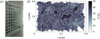
Experimental set-up and image analysis: (a) turbulence generated at grid and network of atomizing jets also serving to seed the flow with sub-Kolmogorov particles at a volume fraction of
 $\widetilde{\unicode[STIX]{x1D719}}_{o}=4.5\times 10^{-5}$
. (b) Typical image where a Voronoï area
 ${\mathcal{A}}_{v}$
is assigned to each particle. Concentration is given by
 ${\mathcal{C}}=1/{\mathcal{A}}_{v}$
, normalized by the background concentration
 ${\mathcal{C}}_{0}=\langle {\mathcal{N}}\rangle /A_{img}$
, where
 $\langle {\mathcal{N}}\rangle$
is the average number of particles per image and
 $A_{img}$
is the image area. Dark colours are dense regions. Contiguous
 ${\mathcal{A}}_{v}$
identify clusters (white outlines).

Inertial particle clusters have been found to scale with the dissipative scales of turbulence, and more specifically with the peak of the vorticity spectrum, for low Reynolds number experiments (Aliseda et al. Reference Aliseda, Cartellier, Hainaux and Lasheras2002; Aliseda & Lasheras Reference Aliseda and Lasheras2006, Reference Aliseda and Lasheras2011). At higher Reynolds numbers and for density ratios close to one, the turbulent scales that are most active in clustering inertial particles can vary significantly and there is a low sensitivity, well below what Kolmogorov scaling would suggest, of the actual size of clusters to turbulent Reynolds numbers (Sumbekova et al. Reference Sumbekova, Cartellier, Aliseda and Bourgoin2017). Various techniques have been developed to quantify inertial particle clustering in turbulence (Sundaram & Collins Reference Sundaram and Collins1997; Bateson & Aliseda Reference Bateson and Aliseda2012; Monchaux, Bourgoin & Cartellier Reference Monchaux, Bourgoin and Cartellier2012). Voronoï tessellations, in particular, provide insights into the local concentration field at the particle scale, without spatial or temporal averaging (Monchaux et al. Reference Monchaux, Bourgoin and Cartellier2010; Obligado et al. Reference Obligado, Teitelbaum, Cartellier, Mininni and Bourgoin2014; Huisman et al. Reference Huisman, Barois, Bourgoin, Chouippe, Doychev, Huck, Morales-Bello, Uhlmann and Volk2016). Dense regions, referred to as clusters are identified from their contiguous Voronoï areas, and the settling velocity of these regions measured experimentally, as a function of turbulent dissipation rate and the residence time of particles interacting with the turbulence. The settling velocity is observed to increase dramatically with cluster size. Increasing cluster concentration is also associated with settling velocity enhancement.
Numerous theoretical formulations have sought to address sedimentation of heavy spheres (Guazzelli & Hinch Reference Guazzelli and Hinch2011). Notably, Hinch (Reference Hinch, Guyan, Nadal and Pomeau1988) proposed a scaling for particle aggregates subjected to statistical fluctuations in local density commensurate with cluster size leading to increasingly large velocity fluctuations. Similarly, Aliseda et al. (Reference Aliseda, Cartellier, Hainaux and Lasheras2002) proposed a model in the context of a turbulent dispersion of heavy particles to estimate terminal velocity as a function of local concentration. Following the volume-average approach of Anderson & Jackson (Reference Anderson and Jackson1967), whereby the equations of motion are derived for continuous particle and fluid phases, we propose a model for the calculation of a flux of particles in the direction of gravity, representing the role of clusters (i.e. collective effects) on the particle dynamics. The aim of this paper is to quantify the role of turbulence in controlling the settling velocity of inertial particles in the flow, through modifications of the instantaneous, local concentration.
Turbulence characteristics at the centre of the wind tunnel where the particle trajectories are analysed. Average longitudinal carrier-phase velocity and fluctuations are
 $U_{0}$
and
 $u^{\prime }$
. The dissipation rate
 $\unicode[STIX]{x1D700}$
was obtained from the longitudinal velocity spectra. The Taylor scale is computed as
 $\unicode[STIX]{x1D706}=\sqrt{15{u^{\prime }}^{2}\unicode[STIX]{x1D708}/\unicode[STIX]{x1D700}}$
, where the gas kinematic viscosity is
 $\unicode[STIX]{x1D708}=1.5\times 10^{-5}$
with
 $Re_{\unicode[STIX]{x1D706}}=u^{\prime }\unicode[STIX]{x1D706}/\unicode[STIX]{x1D708}$
,
 $St=\unicode[STIX]{x1D70F}_{p}/\unicode[STIX]{x1D70F}_{\unicode[STIX]{x1D702}}$
,
 $R=\unicode[STIX]{x1D70F}_{p}g/u^{\prime }$
,
 $\unicode[STIX]{x1D6FE}=a_{\unicode[STIX]{x1D702}}/g$
where
 $a_{\unicode[STIX]{x1D702}}=\unicode[STIX]{x1D700}^{3/2}\unicode[STIX]{x1D708}^{-1/2}$
. The Kolmogorov length, time, and velocity scales are
 $\unicode[STIX]{x1D702}=(\unicode[STIX]{x1D708}^{3}/\unicode[STIX]{x1D700})^{1/4}$
,
 $\unicode[STIX]{x1D70F}_{\unicode[STIX]{x1D702}}=(\unicode[STIX]{x1D708}/\unicode[STIX]{x1D700})^{1/2}$
, and
 $u_{\unicode[STIX]{x1D702}}=(\unicode[STIX]{x1D708}\unicode[STIX]{x1D700})^{1/4}$
.

2 Experimental set-up
Inertial particles in a homogeneous and isotropic, slowly decaying, turbulent gas phase are studied experimentally by injecting a polydisperse liquid droplet population in a wind tunnel (WT) that has been characterized previously (Bateson & Aliseda Reference Bateson and Aliseda2012; Bateson Reference Bateson2016). Briefly, a network of 54 liquid atomizing jets are mounted on the intersections of a
 $9\times 9$
grid (figure 1
a) and serve the dual purpose of generating a distribution of water droplets with no mean spatial concentration gradients and inducing high Reynolds number homogeneous and isotropic turbulence. To avoid coalescence of the individual jets into a single recirculating structure, a supplementary source of momentum along the four walls of the tunnel establishes a nearly uniform velocity profile in the central region of the WT, with very thin (less than 5 % of the tunnel width) boundary layers at the walls. The test section, where the inertial particle interaction with turbulence is studied, is
 $1~\text{m}^{2}$
in cross-section and 5 m in length.
Hot-wire anemometry is used to measure the carrier-flow velocity across the test section. Specifically, a region located at the mid-height, 40 cm from the wall is chosen for all inertial particle measurements, based on velocity statistics at this location showing the single-phase turbulence to be very approximately homogeneous and isotropic. The Taylor-scale Reynolds number
 $Re_{\unicode[STIX]{x1D706}}=220$
remains approximately constant for all three of the downstream locations investigated (see table 1), in agreement with equilibrium similarity theory (Tennekes & Lumley Reference Tennekes and Lumley2000) of WT turbulence in its initial period of decay (Batchelor Reference Batchelor1959) and experimental measurements in the literature (Wells & Stock Reference Wells and Stock1983).
A constant water flux of
 $7.5~\text{l}~\text{min}^{-1}$
is injected through the atomizing jets at a free stream velocity of
 $U_{0}\approx 2.8~\text{m}~\text{s}^{-1}$
resulting in a global volume fraction
 $\widetilde{\unicode[STIX]{x1D719}}_{o}=4.5\times 10^{-5}$
. Phase Doppler Particle Analyser (PDPA) droplet size data are used for the calculation of the particle response time distribution, yielding a mean value of
 $\unicode[STIX]{x1D70F}_{p}=\unicode[STIX]{x1D70C}_{p}\langle d^{2}\rangle /18\unicode[STIX]{x1D707}=4.6~\text{ms}$
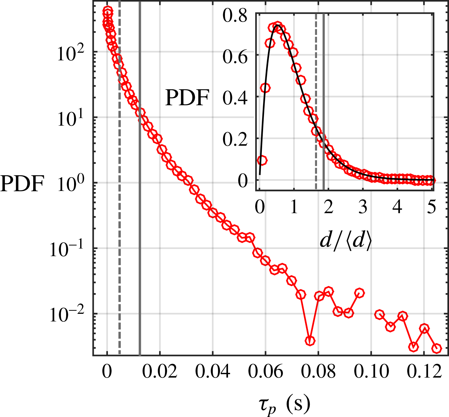
. Figure 2 shows the particle response time corresponding to
 $St=1$
(dashed line) and Sauter diameter (solid line) sized particles. When normalized by the mean diameter,
 $\langle d\rangle =32~\unicode[STIX]{x03BC}\text{m}$
, the associated particle diameter distribution corresponds to a single parameter Gamma distribution (figure 2, inset). The particle size distributions are the same as those studied in Bateson & Aliseda (Reference Bateson and Aliseda2012) and are comparable to those in Aliseda et al. (Reference Aliseda, Cartellier, Hainaux and Lasheras2002) which used a network of similar atomization devices. The present particle size distribution is measured to be approximately stationary throughout the WT, giving local average Stokes numbers:
 $St=[0.60,0.40~0.29]$
. Throughout the paper, brackets refer to values measured at the three WT locations at distances
 $x/M=20,30$
and
 $40$
downstream from the turbulence generating grid.
Flow visualization of the particle trajectories uses high-speed imaging, collecting the light scattered at
 $90^{^{\circ }}$
by the particles illuminated with a high power continuous-wave laser plane aligned with the streamwise and vertical directions in the wind tunnel. The field of view length and width are approximately equal to the integral turbulence length scale (with a 3 : 2 vertical to horizontal aspect ratio), with a thickness of
 $\ell =1~\text{mm}$
, so each image contains
 $O(1000)$
particles. In order to compute fully converged velocity statistics, 5000 independent sequences with 10 consecutive images separated by
 $10^{-4}~\text{s}$
, are collected and analysed with a particle tracking velocimetry algorithm, based on Ouellette, Xu & Bodenschatz (Reference Ouellette, Xu and Bodenschatz2006) and upgraded by Bateson (Reference Bateson2016), to compute the particles’ position and velocity.
Probability density function (PDF) of the particle response time (
 $\unicode[STIX]{x1D70F}_{p}$
) at
 $x/M=20$
, where
 $\unicode[STIX]{x1D70F}_{\unicode[STIX]{x1D702}}=7.7~\text{ms}$
. Inset: particle diameter PDF at the same location. The black solid line corresponds to a Gamma distribution with a single parameter,
 $n=2.1$
. In both, the vertical lines represent an
 $St=1$
particle (dashed) and the Sauter diameter,
 $\langle d^{3}\rangle /\langle d^{2}\rangle =61~\unicode[STIX]{x03BC}\text{m}$
(solid). The arithmetic mean diameter of the distribution is
 $\langle d\rangle =32~\text{m}$
.

3 Experimental characterization of clustering
Voronoï tessellations are used to determine the local concentration of particles. A network of vertices is drawn around each particle in the flow field, such that each point within the resulting cell is closer to the assigned particle than to any other in the field. Thus, each particle is associated with a cell of area
 ${\mathcal{A}}_{v}$
, and the local concentration at each particle location can be defined as
 ${\mathcal{C}}=1/{\mathcal{A}}_{v}$
. Small (large) Voronoï cells with normalized areas
 ${\mathcal{V}}={\mathcal{A}}_{v}/\langle {\mathcal{A}}_{v}\rangle$
that are statistically more probable than a random Poisson process (RPP) are considered to be part of clusters (voids) (Monchaux et al.
Reference Monchaux, Bourgoin and Cartellier2010). Clusters are found as connected sets of normalized areas smaller than
 ${\mathcal{V}}=0.57$
, whereas a value of the normalized areas larger than
 ${\mathcal{V}}=2.1$
is found in the experiments to correspond to voids. These experimental measurements remain constant for the different turbulent conditions presented here, and are consistent with those found in similar experimental configurations (Monchaux et al.
Reference Monchaux, Bourgoin and Cartellier2010; Obligado et al.
Reference Obligado, Teitelbaum, Cartellier, Mininni and Bourgoin2014; Sumbekova et al.
Reference Sumbekova, Cartellier, Aliseda and Bourgoin2017).
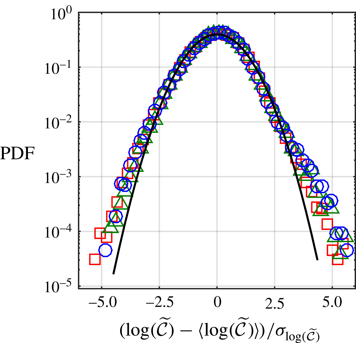
Cluster statistics: PDFs of normalized average cluster concentrations (
 $\widetilde{{\mathcal{C}}}=\langle {\mathcal{C}}\rangle /{\mathcal{C}}_{o}$
) plotted as zero mean, unit variance functions and compared to a Gaussian (black solid line). Data at the different wind tunnel locations
 $x/M=[20,30,40]$
, corresponding to dissipation rates
 $\unicode[STIX]{x1D700}=[0.26,0.11,0.06]~\text{m}^{2}~\text{s}^{-3}$
at
 $Re_{\unicode[STIX]{x1D706}}\approx 220$
and
 $St=[0.60,0.40,0.29]$
, are represented by the symbols [○, ▫, ▵].

The laser sheet width (
 $\ell \sim 2$
–
 $3\unicode[STIX]{x1D702}$
) is assumed to be sufficiently thin to consider illuminated particle aggregates as elementary slices of larger clusters characterized by a linear scale of approximately 10
 $\unicode[STIX]{x1D702}$
(Aliseda et al.
Reference Aliseda, Cartellier, Hainaux and Lasheras2002; Wood, Hwang & Eaton Reference Wood, Hwang and Eaton2005). The quantitative measure of clustering, the standard deviation of Voronoï areas
 $\unicode[STIX]{x1D70E}_{{\mathcal{V}}}$
, is not strongly effected by changing the thickness of the visualization plane from
 $2\unicode[STIX]{x1D702}<\ell <6\unicode[STIX]{x1D702}$
(Monchaux Reference Monchaux2012). Additionally, Voronoï analysis on direct numerical simulations (DNS) data indicates quantitative similarity between two-dimensional (2-D) and 3-D post-processing, suggesting that 2-D slices are an adequate approximation of the 3-D clustering phenomenon (Monchaux Reference Monchaux2012).
The probability density functions of the normalized Voronoï areas,
 ${\mathcal{V}}$
, are known to be log-normal (Monchaux et al.
Reference Monchaux, Bourgoin and Cartellier2010) and this is confirmed in our experiments (data not shown). Log-normality of these PDFs show that the level of clustering can be characterized solely by the standard deviation of the normalized Voronoï areas
 $\unicode[STIX]{x1D70E}_{{\mathcal{V}}}$
: when this measure is larger than that of a 2-D RPP distribution of particles,
 $\unicode[STIX]{x1D70E}_{{\mathcal{V}}}^{RPP}=0.53$
(Ferenc & Zoltan Reference Ferenc and Zoltan2007), clustering is present. Measurements at different conditions with decreasing turbulence dissipation rates yielded values of
 $\unicode[STIX]{x1D70E}_{{\mathcal{V}}}=[1.03,0.96,1.02]\pm 0.08$
, indicating strong clustering (
 $\unicode[STIX]{x1D70E}_{{\mathcal{V}}}>\unicode[STIX]{x1D70E}_{{\mathcal{V}}}^{RPP}$
) throughout the experimental parameter space explored.
Contiguous Voronoï cells with areas lower than a threshold are assembled into clusters, as shown in figure 1(b). The probability distribution of the average concentration in clusters, normalized by the background concentration,
 $\widetilde{{\mathcal{C}}}=\langle {\mathcal{C}}\rangle /{\mathcal{C}}_{o}$
, is approximately log-normally distributed with no clear dependency on the turbulent dissipation rate or residence time in the wind tunnel. The average concentration, over all clusters
 $\langle \log (\widetilde{{\mathcal{C}}})\rangle$
, remains nearly constant throughout the experimental conditions (
 $\langle \log (\widetilde{{\mathcal{C}}})\rangle =[1.43,1.40,1.39]\pm .01$
), but the standard deviation does show a slow evolution with turbulent dissipations rate or residence time:
 $\unicode[STIX]{x1D70E}_{\log \tilde{{\mathcal{C}}}}=[0.37,0.41,0.44]\pm .02$
. The average cluster concentration for all experimental conditions studied here is
 $4.5{\mathcal{C}}_{0}$
, but the concentration in clusters reaches values as high as
 $O(10{\mathcal{C}}_{o})$
, as evidenced by the data in figure 3.
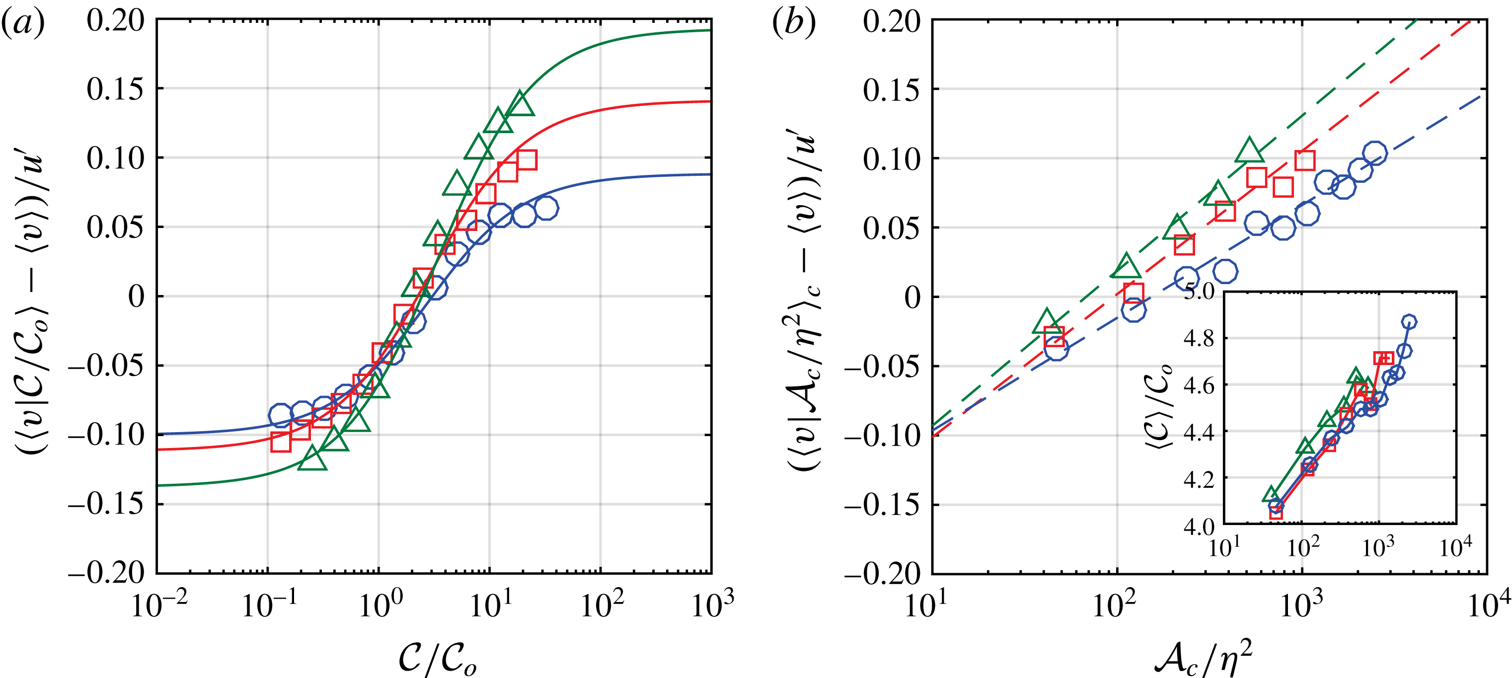
Enhanced settling statistics. Data at the different wind tunnel locations
 $x/M=[20,30,40]$
, corresponding to turbulent fluctuating velocities
 $u^{\prime }=[33,26,24]~\text{cm}~\text{s}^{-1}$
and dissipation rates
 $\unicode[STIX]{x1D700}=[0.26,0.11,0.06]~\text{m}^{2}~\text{s}^{-3}$
at
 $Re_{\unicode[STIX]{x1D706}}\approx 220$
and
 $St=[0.60,0.40,0.29]$
, are represented by the symbols [○, ▫, ▵]. (a) Settling velocity enhancement of particles conditioned on relative concentration with respect to the unconditional settling velocity
 $\langle v\rangle$
and normalized by the fluid velocity fluctuations,
 $u^{\prime }$
. Solid lines correspond to the behaviour predicted by the model (6.1). (b) Cluster settling velocity enhancement with respect to the unconditional average,
 $\langle v\rangle$
, conditioned on normalized cluster area, normalized by the fluid velocity fluctuations. Dashed lines correspond to the predictions by the model in (6.4). Inset: Normalized cluster concentration conditioned on cluster size.

4 Enhanced settling
The settling velocity measured for each particle is conditioned on the local concentration,
 ${\mathcal{C}}/{\mathcal{C}}_{o}$
in figure 4(a). The reference concentration is experimentally measured (
 ${\mathcal{C}}_{o}=2\times 10^{5}~\text{m}^{-2}$
), which can be useful when estimating the associated volume fraction of the conditional statistics presented below:
 $\unicode[STIX]{x1D719}_{o}={\mathcal{C}}_{o}\unicode[STIX]{x03C0}\langle d^{3}\rangle /(6\ell )\sim 1.0\times 10^{-5}$
where
 $\ell =1~$
mm is the laser sheet thickness. This value is reasonably close to the nominal volume fraction
 $\widetilde{\unicode[STIX]{x1D719}}_{o}=4.5\times 10^{-5}$
considering that some particles are too small to be properly detected.
Figure 4(a) shows the particles’ settling velocity conditioned on the local concentration compared to the unconditional settling velocity averaged over all particles,
 $\langle v\rangle$
. The settling velocity of particles increases with local concentration, up to values of 10–20 times the ambient concentration, where the data suggest saturation. The unconditional average value
 $\langle v\rangle$
is found to correspond to the settling rate of regions with a concentration
 ${\mathcal{C}}=2-3{\mathcal{C}}_{o}$
, in agreement with previously published experiments (Aliseda et al.
Reference Aliseda, Cartellier, Hainaux and Lasheras2002) and DNS (Bosse, Kleiser & Meiburg Reference Bosse, Kleiser and Meiburg2006; Monchaux & Dejoan Reference Monchaux and Dejoan2017). This unconditional average settling is large compared to the Stokes settling velocity in a laminar flow, of the order of 2- to 5-fold, and enhancement declines with turbulent dissipation and/or residence time in the wind tunnel:
 $(\langle v\rangle -v_{t})/v_{t}=[1.4,~1.2,~1.0]$
. Settling enhancement scales well with the carrier-phase fluctuations
 $(\langle v\rangle -v_{t})\sim 0.2u^{\prime }$
, as has been found previously (Aliseda et al.
Reference Aliseda, Cartellier, Hainaux and Lasheras2002; Yang & Shy Reference Yang and Shy2003, Reference Yang and Shy2005; Good et al.
Reference Good, Ireland, Bewley, Bodenschatz, Collins and Warhaft2014). It is important to note that discriminating between settling velocity enhancement scaling with the integral scale,
 $u^{\prime }$
, versus the microscale,
 $u_{\unicode[STIX]{x1D702}}$
, has been difficult in past studies due to the similar range of variability in these two metrics. In this experiment, the range over which the integral scale
 $u^{\prime }$
changes compared to the range of variation of the microscale
 $u_{\unicode[STIX]{x1D702}}$
is larger, giving more credence to this scaling of the settling velocity enhancement.
The limit
 ${\mathcal{C}}/{\mathcal{C}}_{o}\ll 1$
gives settling velocities that tend to a constant (
 $w_{v}$
, cf. table 2). We interpret this velocity to be a result of preferential sweeping of isolated particles in the direction of gravity. It decreases with the turbulence dissipation rate:
 $(w_{v}-v_{t})/v_{t}=[0.7,~0.5,~0.2]$
. This element of the settling velocity enhancement is discussed in further detail in the § 6. As particles explore regions with stronger local concentrations their settling velocity rapidly increases until saturating in the densest regions. One could have expected that the increasing role of gravity, measured by a decreasing acceleration ratio (
 $a_{\unicode[STIX]{x1D702}}/g$
, table 1), would induce the dense regions to interact less with the turbulence and thereby settle slower; however, that ignores the strong coupling between particles and between the particle and fluid phases. Maximum enhancement occurs for concentrations of the order of
 $O(30{\mathcal{C}}_{o})$
and correspond to volume fractions
 $\unicode[STIX]{x1D719}\approx 10^{-3}$
, a regime in which four-way coupling may play an important role. Interestingly, the gap between settling velocities at weak (
 ${\mathcal{C}}\sim 10^{-1}{\mathcal{C}}_{o}$
) and strong (
 ${\mathcal{C}}\sim 10{\mathcal{C}}_{o}$
) concentrations is strongest for the lowest turbulent dissipation rates where the residence time of particles in the flow is longest and promotes interaction with the turbulence (figure 4
a). If this enhancement were solely due to preferential concentration of particles in increasingly strong straining regions one would expect the gap to be an increasing function of
 $\unicode[STIX]{x1D700}$
. The opposite tendency is observed which suggests the presence of an additional mechanism to preferential sampling of downward straining regions by the particles. In § 6, this enhancement is interpreted as a result of the enhanced body forces on locally dense regions. The general term ‘collective effects’ refers to enhanced settling velocities due to this mechanism.
Fitting parameters corresponding to locally enhanced settling (6.1) and cluster settling (6.5) velocities for measurements made at
 $x/M=[20,30,40]$
at
 $Re_{\unicode[STIX]{x1D706}}\approx 220$
where the fluid velocity fluctuations are
 $u^{\prime }$
and
 $St=[0.60,0.40,0.29]$
. For (6.1) the parameters include the background flow
 $w_{v}$
as seen by individual particles, particle response time
 $\unicode[STIX]{x1D70F}_{p}$
(held fixed), reference mass fraction
 $\unicode[STIX]{x1D719}_{mo}=\unicode[STIX]{x1D719}_{o}\unicode[STIX]{x1D70C}_{p}/\unicode[STIX]{x1D70C}_{f}$
and the collective effects velocity
 $\widetilde{v}_{tp}=\unicode[STIX]{x1D70F}_{p}g/\unicode[STIX]{x1D719}_{mo}$
. For (6.5) the parameters include the background flow as seen by clusters
 $w_{vc}^{\ast }=w_{vc}+\unicode[STIX]{x1D6FC}\widehat{\unicode[STIX]{x1D70F}}g$
and the cluster collective effects velocity
 $\widetilde{v}_{tc}=\unicode[STIX]{x1D6FC}\unicode[STIX]{x1D6FD}\widehat{\unicode[STIX]{x1D70F}}g$
. The particle number–Voronoï area correlation term,
 $\unicode[STIX]{x1D6FD}$
, evaluated at
 $\langle {\mathcal{A}}_{c}\rangle \simeq 150\unicode[STIX]{x1D702}^{2}$
, the geometrical constant
 $\unicode[STIX]{x1D6FC}$
setting initial velocity enhancement and a modified particle response time
 $\widehat{\unicode[STIX]{x1D70F}}$
(held constant) based on (5.13) assuming steady
 $\unicode[STIX]{x1D719}_{mo}$
at the average cluster concentration are used to evaluate these parameters.

The average settling velocities conditioned on cluster size (
 $\langle v|{\mathcal{A}}_{c}/\unicode[STIX]{x1D702}^{2}\rangle _{c}$
) increase logarithmically with cluster area, as shown in figure 4(b). While the smallest clusters settle slower than the unconditional settling velocity
 $\langle v\rangle$
, clusters larger than
 $O(100\unicode[STIX]{x1D702}^{2})$
settle faster. This size approximately corresponds to the average cluster size, although the physical significance of this threshold is not well understood. Indeed, for a cluster of a given size
 ${\mathcal{A}}_{c}/\unicode[STIX]{x1D702}^{2}$
, the settling velocity enhancement is strongest for the longest residence times, where turbulent fluctuations and dissipation rate are relatively weak. This reinforces the hypothesis that collective effects are a dominant mechanism leading to the enhancement of the settling velocities.
From the inset in figure 4(b), the average concentration in clusters is 4–5
 ${\mathcal{C}}_{o}$
over a wide range of sizes (
 ${\mathcal{A}}_{c}=10^{2}$
–
 $10^{3}~\unicode[STIX]{x1D702}^{2}$
). The average concentration depends logarithmically on cluster size. This dual dependency of the cluster settling velocity and the cluster concentration on cluster size is the key to developing the model for the settling enhancement by collective effects described in the following section. The model behaviour is anticipated by the dashed lines in figure 4(b). The results presented here are the first to establish that the average concentration and cluster area are equivalent measures of particle accumulation, with larger clusters corresponding to more concentrated regions (figure 4
b, inset). The logarithmic dependency requires the large range in
 $\langle {\mathcal{C}}\rangle /{\mathcal{C}}_{o}$
and
 $\langle {\mathcal{A}}_{c}\rangle /\unicode[STIX]{x1D702}^{2}$
reached in these experiments for accurate measurements of this phenomenon.
5 Settling enhancement by collective effects model based on two-fluid averaging
The averaged momentum equations for the particle, fluid and mixture phases are constructed based on Jackson (Reference Jackson2000):
 $$\begin{eqnarray}\displaystyle & \displaystyle \frac{\unicode[STIX]{x2202}}{\unicode[STIX]{x2202}t}(\unicode[STIX]{x1D70C}_{p}\unicode[STIX]{x1D719}\boldsymbol{v})+\unicode[STIX]{x1D735}\boldsymbol{\cdot }(\unicode[STIX]{x1D70C}_{p}\unicode[STIX]{x1D719}\boldsymbol{v}\boldsymbol{v})=\unicode[STIX]{x1D735}\boldsymbol{\cdot }\unicode[STIX]{x1D72B}_{p}+\boldsymbol{f}+\unicode[STIX]{x1D719}\unicode[STIX]{x1D70C}_{p}\boldsymbol{g}, & \displaystyle\end{eqnarray}$$
 $$\begin{eqnarray}\displaystyle & \displaystyle \frac{\unicode[STIX]{x2202}}{\unicode[STIX]{x2202}t}(\unicode[STIX]{x1D70C}_{f}(1-\unicode[STIX]{x1D719})\boldsymbol{u})+\unicode[STIX]{x1D735}\boldsymbol{\cdot }(\unicode[STIX]{x1D70C}_{f}(1-\unicode[STIX]{x1D719})\boldsymbol{u}\boldsymbol{u})=\unicode[STIX]{x1D735}\boldsymbol{\cdot }\unicode[STIX]{x1D72B}_{f}-\boldsymbol{f}+(1-\unicode[STIX]{x1D719})\unicode[STIX]{x1D70C}_{f}\boldsymbol{g}, & \displaystyle\end{eqnarray}$$
 $$\begin{eqnarray}\displaystyle & \displaystyle \frac{\unicode[STIX]{x2202}}{\unicode[STIX]{x2202}t}(\unicode[STIX]{x1D70C}\boldsymbol{w})+\unicode[STIX]{x1D735}\boldsymbol{\cdot }(\unicode[STIX]{x1D70C}\boldsymbol{w}\boldsymbol{w})=\unicode[STIX]{x1D735}\boldsymbol{\cdot }\unicode[STIX]{x1D72B}+\unicode[STIX]{x1D70C}\boldsymbol{g}. & \displaystyle\end{eqnarray}$$
It is important to note that
 $\boldsymbol{v}$
,
 $\boldsymbol{u}$
and
 $\boldsymbol{w}$
correspond to the particle, fluid and mixture phases and do not represent the directional components of the flow velocity. The local volume fraction is denoted by
 $\unicode[STIX]{x1D719}$
, and the momentum equation for the mixture (5.3) is constructed by adding the particle-phase contribution (5.1) to that of the fluid phase (5.2). The barycentric velocity of the mixture phase
 $\boldsymbol{w}=(\unicode[STIX]{x1D70C}_{p}\unicode[STIX]{x1D719}\boldsymbol{v}+\unicode[STIX]{x1D70C}_{f}(1-\unicode[STIX]{x1D719})\boldsymbol{u})/\unicode[STIX]{x1D70C}$
is determined by the locally averaged carrier and disperse-phase velocities,
 $\boldsymbol{u}$
and
 $\boldsymbol{v}$
, using a local mixture density
 $\unicode[STIX]{x1D70C}=\unicode[STIX]{x1D719}\unicode[STIX]{x1D70C}_{p}+(1-\unicode[STIX]{x1D719})\unicode[STIX]{x1D70C}_{f}$
. The right-hand side terms are the effective particle (fluid and mixture) stress tensors,
 $\unicode[STIX]{x1D72B}_{p}$
(
 $\unicode[STIX]{x1D72B}_{f}$
and
 $\unicode[STIX]{x1D72B}=\unicode[STIX]{x1D72B}_{p}+\unicode[STIX]{x1D72B}_{f}$
), the fluid–particle interaction force (
 $\boldsymbol{f}$
) and the specific gravity force.
The effective particle stress tensor contains hydrodynamic, inter-particle, and Brownian contributions, all of which are considered negligible under the dilute, finite particle Stokes number assumptions used here, i.e.
 $\unicode[STIX]{x1D72B}_{p}\sim 0$
. Carrier-phase stress is purely hydrodynamic, with negligible deviatoric contributions Guazzelli & Morris (Reference Guazzelli and Morris2012),
 $$\begin{eqnarray}\unicode[STIX]{x1D72B}_{f}=-(1-\unicode[STIX]{x1D719})p\boldsymbol{I}.\end{eqnarray}$$
The contribution of this term is essential for the fluid–particle interaction,
 $\boldsymbol{f}$
, and is partitioned, per Jackson (Reference Jackson2000):
 $$\begin{eqnarray}\boldsymbol{f}=\unicode[STIX]{x1D719}\unicode[STIX]{x1D735}\boldsymbol{\cdot }\unicode[STIX]{x1D72B}_{f}+n\boldsymbol{f}_{d}.\end{eqnarray}$$
The first term is a particle contribution to the local average pressure gradient, which provides a buoyant resistance of order
 $O(\unicode[STIX]{x1D719})$
by Newton’s third law (Jackson Reference Jackson2000). The second term, weighted by the local particle number density
 $n$
, may contain drag, added-mass and lift contributions, although most often only the drag contribution is considered (Jackson Reference Jackson2000; Guazzelli & Morris Reference Guazzelli and Morris2012). However, the effects of local particle accumulation on drag may be considered to play a separate role from the contributions of overall number density (
 $n_{o}$
) in the generation of drag on the particle phase (Bosse et al.
Reference Bosse, Kleiser and Meiburg2006). Because the standard deviation of the Voronoï areas (and thus local concentration
 ${\mathcal{C}}$
) is of the order of the reference values
 ${\mathcal{C}}_{o}$
, the leading-order contribution to the inter-phase interaction term is hypothesized to result from the reference-number-density-weighted Stokes drag in the isolated particle limit:
 $$\begin{eqnarray}n\boldsymbol{f}_{d}\simeq n_{o}\,\boldsymbol{f}_{d}=n_{o}3\unicode[STIX]{x03C0}\,\text{d}\unicode[STIX]{x1D707}(\boldsymbol{u}-\boldsymbol{v})=\unicode[STIX]{x1D719}_{o}\frac{18\unicode[STIX]{x1D707}}{d^{2}}(\boldsymbol{u}-\boldsymbol{v}).\end{eqnarray}$$
It is clear that (5.1) and (5.2) are not independent of (5.3), and it suffices to consider the momentum equation for the particle and mixture phases. Defining the volume-averaged mixture velocity as
 $\boldsymbol{w}_{v}=\unicode[STIX]{x1D719}\boldsymbol{v}+(1-\unicode[STIX]{x1D719})\boldsymbol{u}$
, the conservation equations for the mixture and particle phases respectively are:
 $$\begin{eqnarray}\displaystyle & \displaystyle \unicode[STIX]{x1D735}\boldsymbol{\cdot }\boldsymbol{w}_{v}=0, & \displaystyle\end{eqnarray}$$
 $$\begin{eqnarray}\displaystyle & \displaystyle \frac{\unicode[STIX]{x2202}\unicode[STIX]{x1D719}}{\unicode[STIX]{x2202}t}+\unicode[STIX]{x1D735}\boldsymbol{\cdot }(\unicode[STIX]{x1D719}\boldsymbol{v})=0. & \displaystyle\end{eqnarray}$$
Note that the volume-averaged mixture velocity
 $\boldsymbol{w}_{v}$
is different from the barycentric velocity
 $\boldsymbol{w}$
of (5.3). By rewriting (5.8) one may obtain:
 $$\begin{eqnarray}\frac{\unicode[STIX]{x2202}\unicode[STIX]{x1D719}}{\unicode[STIX]{x2202}t}+\boldsymbol{w}_{v}\boldsymbol{\cdot }\unicode[STIX]{x1D735}\unicode[STIX]{x1D719}=-\unicode[STIX]{x1D735}\boldsymbol{\cdot }[\unicode[STIX]{x1D719}(\boldsymbol{v}-\boldsymbol{w}_{v})].\end{eqnarray}$$
The evolution of the material derivative of
 $\unicode[STIX]{x1D719}$
is driven by the ability of particles to fall out of the mixture as droplet-laden clusters when a sufficiently high relative velocity is generated. It is this fall-out flux,
 $\boldsymbol{j}_{f}=\unicode[STIX]{x1D719}(\boldsymbol{v}-\boldsymbol{w}_{v})$
, that represents enhanced settling by collective effects in the model.
In order to simplify (5.1) and (5.3), statistical stationarity is assumed and inertial terms are neglected. Consequently, the momentum equations for the particle phase and the mixture become:
 $$\begin{eqnarray}\displaystyle & \displaystyle 0=18\frac{\unicode[STIX]{x1D707}}{d^{2}}\unicode[STIX]{x1D719}_{o}(\boldsymbol{u}-\boldsymbol{v})+\unicode[STIX]{x1D719}(\unicode[STIX]{x1D70C}_{p}-\unicode[STIX]{x1D70C})\boldsymbol{g}, & \displaystyle\end{eqnarray}$$
 $$\begin{eqnarray}\displaystyle & \displaystyle 0=-\unicode[STIX]{x1D735}p+\unicode[STIX]{x1D70C}\boldsymbol{g}. & \displaystyle\end{eqnarray}$$
Notice that the lowest-order (in
 $\unicode[STIX]{x1D719}$
) contribution from buoyancy to (5.10) is simply the hydrostatic pressure needed to support the weight of the mixture,
 $\unicode[STIX]{x1D719}\unicode[STIX]{x1D735}\boldsymbol{\cdot }\unicode[STIX]{x1D72B}_{f}\sim -\unicode[STIX]{x1D719}\unicode[STIX]{x2202}p/\unicode[STIX]{x2202}z=-\unicode[STIX]{x1D719}\unicode[STIX]{x1D70C}g$
. This simple mechanism provides a hydrodynamic coupling between the mixture and the particle phase by the substitution of
 $\boldsymbol{f}=-\unicode[STIX]{x1D719}\unicode[STIX]{x1D70C}\boldsymbol{g}+n_{o}\,\boldsymbol{f}_{d}$
into (5.1). Multiplying both sides of (5.10) by (
 $1-\unicode[STIX]{x1D719}$
), the relative velocity in the Stokes drag term can be rewritten to give an explicit expression for the lowest-order contribution to the fall-out flux that is purely gravitational:
 $$\begin{eqnarray}\boldsymbol{j}_{fo}=\unicode[STIX]{x1D719}_{o}(\boldsymbol{v}-\boldsymbol{w}_{v})=\unicode[STIX]{x1D719}(1-\unicode[STIX]{x1D719})\unicode[STIX]{x1D70F}\boldsymbol{g},\end{eqnarray}$$
and highlights the role of local volume fraction (local concentration) and the particle inertia relative to the flow’s (
 $\unicode[STIX]{x1D70F}=(\unicode[STIX]{x1D70C}_{p}-\unicode[STIX]{x1D70C})d^{2}/18\unicode[STIX]{x1D707}$
) in the enhancement of the settling as the local concentration increases in dense regions. Similar to results using the suspension balance model (Nott, Guazzelli & Pouliquen Reference Nott, Guazzelli and Pouliquen2011; Guazzelli & Morris Reference Guazzelli and Morris2012), the volume-averaging technique employed here, derives an expression for the flux characterizing particle migration.
Considering the right-hand side of the second equality in (5.12) at order
 $O(\unicode[STIX]{x1D719})$
, a dense region (i.e.
 $\unicode[STIX]{x1D719}\rightarrow 1$
) will see a mixture almost entirely composed of the particle phase. In this case,
 $\unicode[STIX]{x1D70F}\rightarrow 0$
suggests that the fluid is relaxing to the particle phase by a process of entrainment. This interpretation is in agreement with two-way coupling simulations (Monchaux & Dejoan Reference Monchaux and Dejoan2017) where the slip velocity attains a value close to the terminal velocity in dense regions. In contrast, in unpopulated regions where
 $\unicode[STIX]{x1D719}\rightarrow 0$
the single particle limit is attained:
 $\unicode[STIX]{x1D70F}\rightarrow \unicode[STIX]{x1D70F}_{p}$
. An empirical form of
 $\unicode[STIX]{x1D70F}$
which has these same properties is:
 $$\begin{eqnarray}\widehat{\unicode[STIX]{x1D70F}}=\unicode[STIX]{x1D70F}_{p}\left(1+\unicode[STIX]{x1D719}_{mo}\frac{\unicode[STIX]{x1D719}}{\unicode[STIX]{x1D719}_{o}}\right)^{-1},\end{eqnarray}$$
where
 $\unicode[STIX]{x1D719}_{mo}=\unicode[STIX]{x1D719}_{o}\unicode[STIX]{x1D70C}_{p}/\unicode[STIX]{x1D70C}_{f}$
is the reference mass loading and the notation
 $\widehat{\unicode[STIX]{x1D70F}}$
is used to distinguish from
 $\unicode[STIX]{x1D70F}$
introduced above. The right-hand side of (5.13) may be thought of as a modified particle response time which accounts for relaxation between particle and fluid phases. This term bears resemblance to the time scale arising in the short relaxation time approximation discussed in Jackson (Reference Jackson2000) which assumes the inertia associated with relative motion between the phases to be negligible, and is valid when
 $\widehat{\unicode[STIX]{x1D70F}}\ll \unicode[STIX]{x1D70F}_{\unicode[STIX]{x1D702}}$
. Note that relaxation between the phases becomes increasingly rapid as local concentration increases and the modified particle response time decreases to some fraction of the Stokes time determined solely by the overall mass loading (
 $\unicode[STIX]{x1D719}_{mo}$
).
From (5.12) and (5.13), the slip velocity between the particle phase and mixture is proportional to
 $\unicode[STIX]{x1D719}/\unicode[STIX]{x1D719}_{o}$
and, thus, a conditional average based on the local relative volume fraction gives an expression for the particle phase:
 $$\begin{eqnarray}\langle \boldsymbol{v}|\unicode[STIX]{x1D719}/\unicode[STIX]{x1D719}_{o}\rangle =\langle \boldsymbol{w}_{v}|\unicode[STIX]{x1D719}/\unicode[STIX]{x1D719}_{o}\rangle +\widehat{\unicode[STIX]{x1D70F}}\boldsymbol{g}\unicode[STIX]{x1D719}/\unicode[STIX]{x1D719}_{o}-O(\unicode[STIX]{x1D719}^{2}).\end{eqnarray}$$
We note that an alternative derivation of (5.14) is possible in the context of the short relaxation time approximation when considering the equations of motion for the difference between (5.2) and (5.1) as well as the mixture (5.3). In what follows, vector notation is dropped and all velocities and fluxes are projected onto gravity’s (vertical) axis:
 $\boldsymbol{g}=|g|\boldsymbol{e}_{z}$
.
6 Discussion
6.1 Locally enhanced settling
The mixture velocity (
 $\langle w_{v}|\unicode[STIX]{x1D719}/\unicode[STIX]{x1D719}_{o}\rangle$
) in (5.14) has an a priori dependence on local volume fraction, but it is not clear how to incorporate this dependency into (5.14). As a first approximation, the mixture velocity is taken to be independent of the local relative volume fraction and is discussed below. The relative number concentration in a cluster or void is considered as a good approximation of the relative volume fraction,
 $\unicode[STIX]{x1D719}/\unicode[STIX]{x1D719}_{o}\simeq ({\mathcal{C}}v_{p}/\ell )/({\mathcal{C}}_{o}v_{p}/\ell )={\mathcal{A}}_{v}^{-1}/{\mathcal{C}}_{o}$
, where
 ${\mathcal{A}}_{v}^{-1}={\mathcal{C}}$
is the experimentally measurable number concentration taken from Voronoï areas,
 $v_{p}$
is the characteristic particle volume and
 $\ell$
is the laser sheet thickness. Under this assumption, the measures of local volume fraction or number concentration are used interchangeably. The resulting model yields:
 $$\begin{eqnarray}\langle v|\unicode[STIX]{x1D719}/\unicode[STIX]{x1D719}_{o}\rangle =w_{v}+\frac{\unicode[STIX]{x1D719}}{\unicode[STIX]{x1D719}_{o}}v_{t}\left(1+\unicode[STIX]{x1D719}_{mo}\frac{\unicode[STIX]{x1D719}}{\unicode[STIX]{x1D719}_{o}}\right)^{-1},\end{eqnarray}$$
where a function of
 $\unicode[STIX]{x1D719}/\unicode[STIX]{x1D719}_{o}$
is fit to the data in figure 4(a). Three fitting parameters are present in (6.1):
 $w_{v}$
,
 $v_{t}=\unicode[STIX]{x1D70F}_{p}g$
and
 $\unicode[STIX]{x1D719}_{mo}=\unicode[STIX]{x1D719}_{o}\unicode[STIX]{x1D70C}_{p}/\unicode[STIX]{x1D70C}_{f}$
, as tabulated in table 2. The latter two parameters are measurable while the former is experimentally inaccessible. Note that
 $v_{t}$
is constant throughout the WT due to the stationarity of the particle size distribution.
In the dilute limit when
 $\unicode[STIX]{x1D719}/\unicode[STIX]{x1D719}_{o}\rightarrow 0$
, (6.1) simplifies to
 $\langle v|\unicode[STIX]{x1D719}/\unicode[STIX]{x1D719}_{o}\rangle \simeq w_{v}$
and particle settling is governed solely by the volume-averaged mixture velocity. From (5.7), the mixture is incompressible, which implies that regions of strong downward volume flux must be compensated by a back-flow elsewhere. Such fluxes may be associated locally with confinement or to entrainment due to sedimentation. The resulting back-flow may be thought of as filling the interstitial regions between dense regions with a mixture ‘headwind’, formed mostly by carrier phase (recall that
 $w_{v}=v\unicode[STIX]{x1D719}+u(1-\unicode[STIX]{x1D719})$
). This consistent with the data shown in figure 4(a), where strong enhancement for the low dissipation/high residence time experiments begets depressed values of
 $w_{v}$
. As a result,
 $w_{v}$
is interpreted as the local contribution of a back-flow which may arise due to the incompressibility of the mixture phase. We assume that
 $w_{v}$
is applied uniformly over the observation region to enhance the particle settling velocity and is independent of local concentration. Note that
 $w_{v}$
is not a quantity that can be measured directly, and its role in the sedimentation process is subject to further understanding that requires explicit experimental measurements.
In highly concentrated regions,
 $\unicode[STIX]{x1D719}\gg \unicode[STIX]{x1D719}_{o}$
, (6.1) takes the asymptotic form:
 $$\begin{eqnarray}\langle v|\unicode[STIX]{x1D719}/\unicode[STIX]{x1D719}_{o}\rangle =w_{v}+\widetilde{v}_{tp}.\end{eqnarray}$$
The first term on the right-hand side is the background flow described above while the second term represents the contribution of the collective effects velocity
 $\widetilde{v}_{tp}=v_{t}/\unicode[STIX]{x1D719}_{mo}$
which is strictly determined by the composition of the mixture: overall mass fraction (
 $\unicode[STIX]{x1D719}_{mo}=\unicode[STIX]{x1D719}_{o}\unicode[STIX]{x1D70C}_{p}/\unicode[STIX]{x1D70C}_{f}$
) and the Stokes velocity (
 $v_{t}=\unicode[STIX]{x1D70F}_{p}g$
). Because
 $\unicode[STIX]{x1D70F}_{p}$
is constant, increases in
 $\widetilde{v}_{tp}$
result from a decrease in the overall mass fraction, or a loss in mass in the particle phase which is coherent with the cumulative effect of the sedimentation process. Although enhanced collective effects at weak mass loading may seem paradoxical, it may be understood by the delay in the mechanism which decreases the effective particle response time
 $\widehat{\unicode[STIX]{x1D70F}}$
with respect to its nominal value
 $\unicode[STIX]{x1D70F}_{p}$
in (5.13). Initial settling velocity increases are linear in
 $\unicode[STIX]{x1D719}/\unicode[STIX]{x1D719}_{o}$
, which corresponds to the Stokes drag (proportional to
 $\unicode[STIX]{x1D719}_{o}$
) compensating the excess body force due to particle accumulation (proportional to
 $\unicode[STIX]{x1D719}$
) as given by (5.10). If the reference mass loading is small then a large relative volume fraction is required to generate the required buoyant drag to reduce the particle response time by a given amount. Likewise, if the mass loading is large then
 $\unicode[STIX]{x1D719}_{mo}\unicode[STIX]{x1D719}/\unicode[STIX]{x1D719}_{o}\sim O(1)$
for smaller relative volume fractions in (5.13), precipitating a decrease in
 $\widehat{\unicode[STIX]{x1D70F}}$
and ultimately smaller values of
 $\widetilde{v}_{tp}$
. The term coupling the particle and carrier phases via the pressure gradient contribution to (5.13) is fundamental in capturing the settling rate saturation observed in figure 4(a).
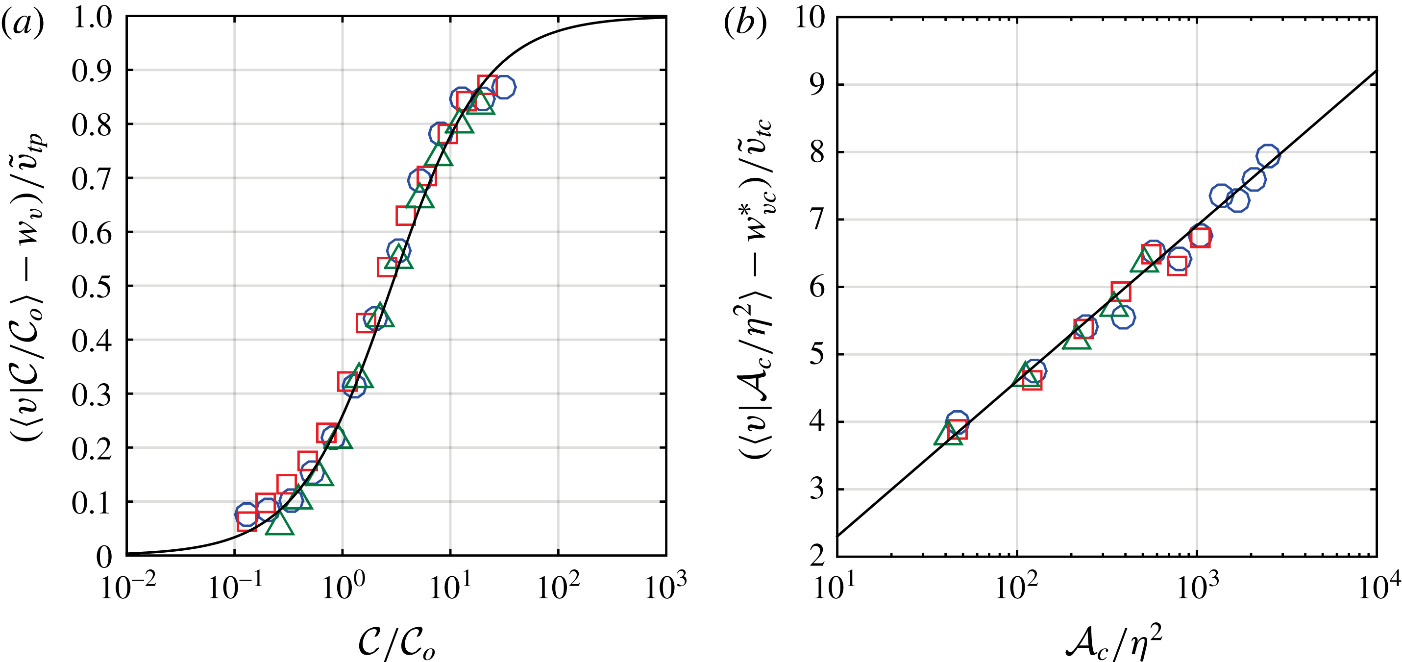
Normalized settling velocity enhancement due to collective effects. Parameters are as given in figure 4. (a) Local settling enhancement with respect to the volume average mixture velocity
 $w_{v}$
and the collective effects velocity
 $\widetilde{v}_{tp}=\unicode[STIX]{x1D70F}_{p}g/\unicode[STIX]{x1D719}_{mo}$
. The solid black line is a fit of (6.1). (b) Cluster settling enhancement with respect to the modified volume-averaged mixture velocity
 $w_{vc}^{\ast }=w_{vc}+\unicode[STIX]{x1D6FC}V_{t}$
and cluster collective effects velocity
 $\widetilde{v}_{tc}=\unicode[STIX]{x1D6FC}\unicode[STIX]{x1D6FD}V_{t}$
(see § 6.2). The solid line corresponds to a fit of (6.5).

Subtracting
 $\langle w_{v}\rangle$
from (6.1) and normalizing by
 $\widetilde{v}_{tp}$
gives the solid black curve in figure 5(a). Applying the same procedure to the data demonstrates that the model equation describes the measurements well. Figure 5(a) depicts the normalized enhanced settling velocity at the particle level due to collective effects. The value
 $\unicode[STIX]{x1D719}_{mo}$
used as a fitting parameter (cf. table 2) is at the lower bound of the fit’s 99 % confidence interval, which corresponds to a volume fraction approximately 7–9 times the reference value of
 $\widetilde{\unicode[STIX]{x1D719}}_{o}=4.5\times 10^{-5}$
. This fitted parameter is considered a reasonable approximation of the reference value considering that the densest regions correspond to local volume fractions of the order of
 $30\widetilde{\unicode[STIX]{x1D719}}_{o}$
. Interestingly, the monotonically decreasing fitting parameter
 $\unicode[STIX]{x1D719}_{mo}$
evolves approximately like the number of particles per image (decreasing nearly 30 % between
 $x/M=20$
and 40). A decrease in the overall mass loading with downstream location may be inferred and is coherent with the increasing gap between settling velocities in low and high concentrations that results from weakening buoyant resistance to high concentration regions. We believe this to be evidence of the dominant role of collective effects in enhancing settling velocities with respect to mechanisms such as preferential sampling that would predict this gap to decrease rather than increase with decreasing
 $\unicode[STIX]{x1D700}$
(increasing residence time in the wind tunnel).
6.2 Enhanced settling in clusters
Clusters are identified as described previously (see § 3) and in general correspond to structures with average concentrations higher than, but of the order of,
 ${\mathcal{C}}_{o}$
:
 $\langle {\mathcal{C}}\rangle /{\mathcal{C}}_{o}\gtrsim 1$
. The average concentration in a cluster of area
 ${\mathcal{A}}_{c}$
containing
 ${\mathcal{N}}$
particles can be expressed by:
 $$\begin{eqnarray}\langle {\mathcal{C}}({\mathcal{A}}_{c})\rangle \simeq {\mathcal{C}}_{o}+\frac{\langle {\mathcal{N}}\rangle }{{\mathcal{A}}_{c}}\left(1-\frac{\langle {\mathcal{N}}^{\prime }{\mathcal{A}}_{v}^{\prime }\rangle }{\langle {\mathcal{N}}\rangle \langle {\mathcal{A}}_{v}\rangle }\right),\end{eqnarray}$$
where the subscripts
 $c/v$
refer to clusters/Voronoï areas. A Reynolds decomposition has been applied to
 ${\mathcal{C}}({\mathcal{A}}_{c})={\mathcal{N}}/\sum _{1}^{N}{\mathcal{A}}_{v}$
and
 ${\mathcal{A}}_{c}\approx \sum _{1}^{N}\langle {\mathcal{A}}_{v}\rangle$
. The term in parenthesis
 $\unicode[STIX]{x1D6FD}({\mathcal{A}}_{c})=(1-\langle {\mathcal{N}}^{\prime }{\mathcal{A}}_{v}^{\prime }\rangle /\langle {\mathcal{N}}\rangle \langle {\mathcal{A}}_{v}\rangle )$
is evaluated experimentally (not shown) and is an increasing function of cluster size. Its correlation term is near unity for the smallest clusters (
 $\unicode[STIX]{x1D6FD}({\mathcal{A}}_{c})\simeq 0$
) and saturates to a positive, non-zero value for the largest. Large correlations are indicative of growing inter-particle distances within clusters (measured by positive
 ${\mathcal{A}}_{v}^{\prime }$
), and therefore of cluster growth, corresponding to a rapid accumulation of particles (measured by positive
 ${\mathcal{N}}^{\prime }$
). Indeed, in figure 4(b, inset), cluster growth occurs in such a way as to increase particle concentration with respect to the background value.
It can be seen in the inset of figure 4(b) that the average concentration in clusters
 $\langle {\mathcal{C}}\rangle /{\mathcal{C}}_{o}$
depends logarithmically on the normalized cluster area
 ${\mathcal{A}}_{c}/\unicode[STIX]{x1D702}^{2}$
. Based on this experimental observation, the second term on the right-hand side of (6.3) is written as
 $\unicode[STIX]{x1D6FD}\log ({\mathcal{A}}_{c}/\unicode[STIX]{x1D702}^{2})$
where
 $\unicode[STIX]{x1D6FD}=\unicode[STIX]{x1D6FD}(\langle {\mathcal{A}}_{c}\rangle )$
is evaluated for the average cluster size,
 $\langle {\mathcal{A}}_{c}\rangle \simeq 150\unicode[STIX]{x1D702}^{2}$
, for each experimental condition. When taking
 $\langle {\mathcal{C}}\rangle /{\mathcal{C}}_{o}$
from (6.3) and substituting it into (5.14) one obtains:
 $$\begin{eqnarray}\langle v|{\mathcal{A}}/\unicode[STIX]{x1D702}^{2}\rangle _{c}=w_{vc}+\unicode[STIX]{x1D6FC}V_{t}(1+\unicode[STIX]{x1D6FD}\log ({\mathcal{A}}_{c}/\unicode[STIX]{x1D702}^{2})),\end{eqnarray}$$
where the subscript
 $\langle \boldsymbol{\cdot }\rangle _{c}$
indicates that the velocity is averaged inside clusters. The incipient cluster settling velocity is
 $\unicode[STIX]{x1D6FC}V_{t}=\unicode[STIX]{x1D6FC}\widehat{\unicode[STIX]{x1D70F}}g$
, with
 $\widehat{\unicode[STIX]{x1D70F}}$
equal to the effective particle response time in (5.13) assuming steady
 $\unicode[STIX]{x1D719}_{mo}$
, evaluated at the most probable cluster’s concentration and using the value of
 $\unicode[STIX]{x1D70F}_{p}$
determined from figure 2. The geometrical constant
 $\unicode[STIX]{x1D6FC}$
, which is of order
 $O(1)$
and sets the initial increase of
 $\langle v|{\mathcal{A}}_{c}/\unicode[STIX]{x1D702}^{2}\rangle _{c}$
, is estimated by extrapolating the data in figure 4(b, inset) to
 ${\mathcal{A}}_{c}/\unicode[STIX]{x1D702}^{2}\sim 1$
, as given in table 2. The interpretation of
 $w_{vc}$
is similar to that of
 $w_{v}$
and represents the contribution of a background flow to the settling velocity of clusters. For simplicity, we consider a single background contribution
 $w_{vc}^{\ast }=w_{vc}+\unicode[STIX]{x1D6FC}V_{t}$
. Thus, (6.4) presents two fitting parameters,
 $w_{vc}^{\ast }$
and a velocity we refer to as the cluster collective effects velocity
 $\widetilde{v}_{tc}=\unicode[STIX]{x1D6FC}\unicode[STIX]{x1D6FD}V_{t}$
(see table 2) which gives the following simplified equation:
 $$\begin{eqnarray}\langle v|{\mathcal{A}}/\unicode[STIX]{x1D702}^{2}\rangle _{c}=w_{vc}^{\ast }+\widetilde{v}_{tc}\log ({\mathcal{A}}_{c}/\unicode[STIX]{x1D702}^{2}).\end{eqnarray}$$
In the limit where
 ${\mathcal{A}}_{c}\sim \unicode[STIX]{x1D702}^{2}$
, particles are distributed in such a way that the local concentration is approximately
 ${\mathcal{C}}_{o}$
. Collective effects do not play a role and clustered particles are swept downward by the advective background flow in much the same manner as individual particles. Indeed, the background flow velocity
 $w_{vc}^{\ast }$
measured in the clustering case is close to that of the individual particle case
 $w_{v}$
, and have a similar dependence on the fluid velocity fluctuations:
 $w_{vc}^{\ast }=0.17u^{\prime }$
(as compared with
 $w_{v}=0.25u^{\prime }$
). We note that
 $w_{v}$
was measured based on the limit
 ${\mathcal{C}}\ll {\mathcal{C}}_{o}$
while
 $w_{vc}^{\ast }$
is measured where
 ${\mathcal{C}}\sim {\mathcal{C}}_{o}$
. It is not apparent that the difference between
 $w_{v}$
and
 $w_{vc}^{\ast }$
is significant as it is smaller than the terminal velocity,
 $\unicode[STIX]{x1D70F}_{p}g$
. From the discussion in § 6.1, the background flow is thought to apply equally to dense and sparsely populated zones, which would indicate that
 $w_{vc}^{\ast }$
and
 $w_{v}$
may be substantially the same.
In the limit
 ${\mathcal{A}}_{c}\gg \unicode[STIX]{x1D702}^{2}$
, collective effects generate increasing sedimentation velocities for larger and larger clusters. Figure 5(b) shows the settling enhancement due to collective effects, as a function of cluster size. The rate at which collective effects generate increases in settling velocities is set by the cluster collective effects velocity,
 $\widetilde{v}_{tc}=\unicode[STIX]{x1D6FC}\unicode[STIX]{x1D6FD}V_{t}$
, which in turn is governed by the particle number–Voronoï area correlation
 $\unicode[STIX]{x1D6FD}$
for a given distribution of particle sizes (holding
 $\unicode[STIX]{x1D6FC}V_{t}$
fixed). This term reflects the ability of a growing cluster to entrain new particles. When calculated experimentally,
 $\unicode[STIX]{x1D6FD}$
is not seen to change with experimental conditions (turbulent dissipation rate or residence times in the WT) and, consequently, is insensitive to the varying average Stokes number. This is reminiscent of the absence of Stokes number dependence in the enhanced settling statistics conditioned on local relative concentration in Aliseda et al. (Reference Aliseda, Cartellier, Hainaux and Lasheras2002), which was interpreted to be the signature of collective effects. It is possible that the Reynolds number is an important parameter in determining
 $\unicode[STIX]{x1D6FD}$
, though investigation of this dependency is not possible in the current experimental configuration.
7 Conclusion
A polydisperse distribution of inertial particles in a turbulent wind tunnel with decaying turbulence (dissipation rate decreasing slowly with distance downstream) at constant Reynolds number has been studied. Experimental measurements of particle size, concentration and vertical velocity have been collected to investigate inertial particle settling and clustering. Voronoï area analysis provides evidence of local particle accumulation with local fluctuations reaching an order of magnitude increase with respect to the background volume fraction.
Particle settling velocities conditioned on the local volume fraction manifest three regimes. First, for the smallest local volume fractions (
 $\unicode[STIX]{x1D719}\leqslant 10^{-6}$
), particles are isolated and responsive to a general background flow which is associated with settling-induced advective currents. Second, at intermediate volume fractions near the reference value
 $\widetilde{\unicode[STIX]{x1D719}}_{o}\sim 4.5\times 10^{-5}$
, particles experience a settling velocity enhancement proportional to turbulence fluctuations, which is suggestive of preferential sweeping. As particles begin to cluster, a third regime is attained where rapid settling velocity increases saturate when the local volume fraction nears
 $\unicode[STIX]{x1D719}=10^{-4}$
–
 $10^{-3}$
. This is a novel observation and presents a limit to the settling velocity enhancement at approximately 60 %–100 % of the values measured in low density regions. The corresponding gap between settling velocities at low and high densities increases with decreasing turbulent kinetic energy dissipation rate. Were these increases due to a mechanism such as preferential sweeping, one would expect proportionality with turbulence dissipation rates. The opposite trend is observed both at the particle and cluster level, which represents our strongest evidence for the role of collective effects in the enhancement of settling velocities: the generation of excess downward forces on locally dense regions.
A new model is derived from first principles following a two-fluid approach in order to determine the role of local concentration in enhanced settling rates. Initial enhancement in settling is due to the predominance of gravitational effects with respect to the Stokes drag in the momentum balance. The particle phase is coupled to the carrier phase by the pressure gradient (hydrostatic to first approximation) which provides a buoyant resistance to the particle phase in locally dense regions and accounts for the observed saturation in settling enhancement. An effective particle response time (
 $\widehat{\unicode[STIX]{x1D70F}}$
) is introduced that can reach a fraction of the nominal value when
 $\unicode[STIX]{x1D719}\gg \unicode[STIX]{x1D719}_{o}$
, indicating that the carrier phase relaxes to the particle phase in such regions, and is indicative of two-way coupling. No turbulence parameters appear explicitly in the model, indicating that it may have applications in particle-laden flows beyond the case of turbulence–particle interactions examined here. The average particle concentration in clusters increases logarithmically with cluster size, a new and non-trivial result. The particle number–Voronoï area correlation
 $\unicode[STIX]{x1D6FD}$
helps to understand this evolution while simultaneously determining the settling enhancement in clusters.
This study has significant implications for the mechanisms governing the coalescence of droplets or the coagulation of inertial particles due to turbulence-induced collisions. Clusters may act as large collector particles trapping smaller particles due to their larger settling velocity (Pruppacher & Klett Reference Pruppacher and Klett2004). Trapped particles then find themselves in environments where the volume fraction is up to 10 times that of the surrounding fluid, leading to increased collisions (Sundaram & Collins Reference Sundaram and Collins1997). This process may decrease the time for cloud particles to close the size gap and attain runaway growth and the millimetric size of raindrops observed in warm rain events (Pruppacher & Klett Reference Pruppacher and Klett2004).
Acknowledgements
A.A. and C.B. acknowledge support from the National Science Foundation (Award NSF-0731248). P.D.H. and R.V. acknowledge the support of the research programs ANR-13-BS09-0009 and PALSE/2013/26. The LEGI laboratory is part of the LabEx TEC 21(Investissements d’Avenir, grant agreement ANR-11-LABX-0030). Contribution from the European project EuHIT – European High-performance Infrastructures in Turbulence – is also acknowledged.