2.1. Governing equations

An interface-capturing DIM (Anderson, McFadden, and Wheeler 1998; Jamet et al. Reference Jamet, Lebaigue, Coutris and Delhaye2001) is employed in this study by combining a multicomponent flow model with a shock-capturing finite-volume method. These techniques are referred to as DIMs, as they do not explicitly track sharp interfaces, allowing for numerical diffusion at the interface. The DIM has been commonly used for modelling transcritical flows as it aligns well with observations that the interface thickness increases near the critical point (Ma, Lv, and Ihme Reference Ma, Yu and Matthias2017; Bravo et al. Reference Bravo, Peter, Matthias and Kevin2018; Ma Reference Ma, Wu, Banuti and Ihme2019; Ma, Wu, Banuti et al. Reference Ma, Wu, Banuti and Ihme2019). This approach ensures conservation, and thermodynamic consistency in mixture cells, and handles dynamically appearing or disappearing interfaces. The DIM offers several advantages over sharp-interface methods (SIMs) such as volume-of-fluid (VOF, Li, Renardy, and Renardy Reference Li, Yuriko and Michael2000; Sun & Tao Reference Sun and Tao2010), front-tracking (Unverdi & Tryggvason Reference Unverdi and Grétar1992; Tryggvason et al. Reference Tryggvason, Bernard, Asghar, Damir, Al-Rawahi, Tauber, Han, Nas and Jan2001; Terashima & Tryggvason Reference Terashima and Grétar2009) and level-set methods (Chang et al. Reference Chang, Hou, Merriman and Osher1996; Sussman & Puckett Reference Sussman and Elbridge2000). The SIM often involves loss of mass conservation and requires implementing complex interfacial boundary conditions. In addition, adapting the SIM to compressible supercritical flows involving phase change proves highly complex (Fuster Reference Fuster2019). Moreover, the DIM typically offers higher efficiency compared with its interface-tracking counterparts, which is crucial for addressing multiscale problems. In this study, a 2-D compressible, multiphase and multicomponent model of immiscible fluids in mechanical equilibrium is developed to consider the effects of surface tension and viscosity on transcritical breakup. The governing equations for a diffuse interface two-species system are as follows:

(2.1) \begin{align} \frac{\partial \rho }{\partial t} &+\boldsymbol{\nabla }\boldsymbol{\cdot }\left(\rho \boldsymbol{u}\right)=0, \end{align}

(2.2) \begin{align} \frac{\partial \left(\alpha _{D}\rho \right)}{\partial t} &+\boldsymbol{\nabla }\boldsymbol{\cdot }\left(\alpha _{D}\rho \boldsymbol{u}\right)=0, \end{align}

(2.3) \begin{align} \frac{\partial \left(\rho \boldsymbol{u}\right)}{\partial t}+\boldsymbol{\nabla }\boldsymbol{\cdot } & \left(\rho \boldsymbol{u}\otimes \boldsymbol{u}+p\boldsymbol{I}-\boldsymbol{T}\right)=\sigma \kappa \boldsymbol{\nabla }\alpha _{D}, \end{align}

(2.4) \begin{align} \frac{\partial E}{\partial t}+\boldsymbol{\nabla }\boldsymbol{\cdot } & \left(\boldsymbol{u}\left(E+p\right)-\boldsymbol{T}\boldsymbol{\cdot }\boldsymbol{u}\right)=\sigma \kappa \boldsymbol{u}\boldsymbol{\cdot }\boldsymbol{\nabla }\alpha _{D}, \end{align}

where $\alpha _{D}$ and $\alpha _{s}$ are the volume fraction of the droplet fluid species and the surroundings, respectively. Here $\rho$ is the density, $\boldsymbol{u}$ is the velocity vector, $p$ is the pressure, $\boldsymbol{T}$ is the viscous stress tensor, $E$ is the total energy defined as $E=\rho (e+({| \boldsymbol{u}| ^{2}}/{2}))$ , where $e$ is the internal energy, $\sigma$ is the surface tension coefficient, $\kappa$ is the local interface curvature and $\boldsymbol{I}$ is the identity matrix. The viscous stress tensor is given as $\boldsymbol{T}=2\mu (\boldsymbol{D}-({1}/{3})(\boldsymbol{\nabla }\boldsymbol{\cdot }\boldsymbol{u})\boldsymbol{I})$ , where $\mu$ is the viscosity and $\boldsymbol{D}=({1}/{2})(\boldsymbol{\nabla }\boldsymbol{u}+(\boldsymbol{\nabla }\boldsymbol{u})^{T})$ is the deformation rate tensor. The second (bulk) viscosity is not considered. The mass fraction of the second species of the two-component system (D and S representing the droplet and the surrounding fluids, respectively) is given by the mixture rule $\alpha _{S}=1-\alpha _{D}$ . Two different systems of equations are employed to close the system for which the mixing rules are described in Appendices A1–A3. The surface tension is implemented as a volume force through the continuum surface force (CSF) model following the method suggested by Garrick et al. (Reference Garrick, Mark and Jonathan2017). The source terms on the right-hand side of (2.3) and (2.4) consider the surface tension effects (Perigaud and Saurel Reference Perigaud and Richard2005; Garrick, Owkes, and Regele Reference Garrick, Mark and Jonathan2017) with an induced pressure jump calculated as ${\Delta} p_{k}=\sigma \kappa {\Delta} \alpha _{D}$ . The local interface curvature ( $\kappa$ ) is determined using the interface normal that is described as a function of the mass fraction as $\kappa =-\boldsymbol{\nabla }\boldsymbol{\cdot }\boldsymbol{n}=-\boldsymbol{\nabla }\boldsymbol{\cdot }({\boldsymbol{\nabla }\alpha _{D}}/{| \boldsymbol{\nabla }\alpha _{D}| })$ . The curvature is calculated by computing the normal vector ( $\boldsymbol{n}$ ) using the fourth-order central difference method. A second-order central difference scheme is employed to determine the curvature. Finally, the curvature is extended outwards from the interface centre ( $\alpha _{D}=0.5$ ) using 10 iterations of the filtering procedure (Garrick, Owkes, and Regele Reference Garrick, Mark and Jonathan2017). Additionally, the Harten–Lax–van Leer-contact (HLLC) flux is modified to include the pressure jump due to the capillary force following the procedure outlined in Garrick, Owkes, and Regele (Reference Garrick, Mark and Jonathan2017). Prior studies have used compressible flow models with both conservative and non-conservative models for surface force (Perigaud and Saurel Reference Perigaud and Richard2005; Braconnier and Nkonga Reference Braconnier and Boniface2009; Le Martelot, Saurel & Nkonga Reference Le Martelot, Saurel and Nkonga2014; Shukla Reference Shukla2014). It is noted that in this study, the non-conservative form of the CSF model is chosen, which enables flexible treatment of the curvature term without a loss in accuracy. This formulation computes the surface tension as a volumetric force based on the gradient of the volume fraction $\alpha _{D}$ . The normal vector and curvature at the interface are calculated directly from $\alpha _{D}$ , making the uniformity of $\alpha _{D}$ crucial for accurate results. To mitigate the distortions in the $\alpha _{D}$ field and ensure accurate curvature computation, we incorporated the tangent of hyperbola interface-capturing (THINC) method (Garrick, Hagen, and Regele Reference Garrick, Wyatt and Jonathan2017). This method sharpens the interface and reduces numerical diffusion, thereby improving the representation of $\alpha _{D}$ gradients. The curvature calculation utilises a four-point quadrature formulation introduced by Garrick, Owkes, and Regele (Reference Garrick, Mark and Jonathan2017), which has been shown to improve accuracy by considering higher-order variations in $\alpha _{D}.$ As we will show in this study, the choice of $\alpha _{D}$ imposes minimal impact on the detected breakup modes.

The ST-EoS is given in (2.5) as follows:

(2.5) \begin{equation}\varGamma p+\varPi =E-\frac{1}{2}\rho \left| \boldsymbol{u}\right| ^{2}.\end{equation}

Here $\varGamma ={1}/{\gamma -1}$ , $\varPi ={\gamma \pi _{\infty }}/{\gamma -1}$ , $\gamma$ and $\pi _{\infty }$ are fluids properties.

The PR-EoS (Peng and Robinson Reference Peng and Donald1976) is as follows:

(2.6) \begin{equation}p=\frac{R_{U}T}{V_{m}-b}-\frac{a}{V_{m}^{2}+2bV_{m}-b^{2}}.\end{equation}

Here $T$ is the temperature, $R_{U}$ is the universal gas constant, $V_{m}$ is the molar volume defined as $V_{m}={M}/{\rho }$ , $M$ is the molar mass and $a$ and $b$ are coefficients that depend on the state and composition of the fluid. The mixing rules are selected based on the suggestions given by Ma et al. (Reference Ma, Yu and Matthias2017). The coefficients $a$ and $b$ in (2.6) are evaluated as $a=\sum_{D=1}^{2}\,\sum _{S=1}^{2}\,\alpha _{D}\alpha _{S}a_{\textit{DS}} \text{ and }b=\sum _{D=1}^{2}\,\alpha _{D}b_{D}$ , where the coefficients $a_{\textit{DS}}$ and $b_{D}$ are calculated using the following equations (D and S representing the droplet and surrounding fluids, respectively):

(2.7) \begin{align} a_{\textit{DS}} &=0.457236\frac{\left(RT_{\textit{c,DS}}\right)^{2}}{p_{\textit{c,DS}}}\left(1+c_{\textit{DS}}\left(1-\sqrt{\frac{T}{T_{\textit{c,DS}}}}\right)\right)^{2}, \qquad b_{D}=0.077796\frac{RT_{\textit{c,D}}}{p_{\textit{c,D}}}; \end{align}

(2.8) \begin{align} c_{\textit{DS}} &=0.37464+1.54226\omega _{\textit{DS}}-0.26992\omega _{\textit{DS}}^{2}. \end{align}

The critical mixture conditions for temperature, pressure, molar volume, compressibility and acentric factors are determined as

(2.9) \begin{align} T_{\textit{c,DS}} &=\sqrt{T_{\textit{c,D}}T_{c,S}}\left(1-k_{\textit{DS}}\right), \qquad \!\!\!\! p_{\textit{c,DS}}=Z_{\textit{c,DS}}\frac{RT_{\textit{c,DS}}}{v_{\textit{c,DS}}},\qquad \!\!\!\! v_{\textit{c,DS}}=\frac{1}{8}\left(v_{\textit{c,D}}^{\tfrac{1}{3}}+v_{c,S}^{\tfrac{1}{3}}\right)^{3}; \end{align}

(2.10) \begin{align} Z_{\textit{c,DS}} &=\frac{1}{2}\left(Z_{\textit{c,D}}+Z_{c,S}\right),\qquad \omega _{\textit{DS}}=\frac{1}{2}\left(\omega _{D}+\omega _{S}\right), \end{align}

where R is the universal gas constant, $T_{c}$ is the critical temperature, $p_{c}$ is the critical pressure, $v_{c}$ is the critical molar volume, $Z_{c}$ is the critical compressibility factor, $k_{\textit{DS}}$ is the binary interaction parameter and $\omega$ is the acentric factor. The parameters for the NASA polynomials used to determine the internal energy, enthalpy and entropy are adopted from McBride (Reference McBride1993). The PR-EoS is modified to approximate the state of the fluid in the vapour dome region to increase the robustness of the numerical method following a method suggested by Knudsen et al. (Reference Knudsen, Doran, Mittal, Meng and Spurlock2017) and outlined in Appendix A2. Phase separation can occur at the interface; however, the approximation has an insignificant influence on the shock transmission across the fluid interface as these regions are small. At such conditions, if the temperature becomes relatively low, the equation of state returns negative pressures and the speed of sound may become complex valued in the vapour dome for certain density values. To remedy these problems, the pressure is given by an approximate saturation pressure of the mixture that limits the speed of sound to 1 ms⁻¹. The modified PR-EoS approach is an alternative approach to the vapour–liquid equilibrium method commonly used to account for phase separation that poses significant complexities and additional computational costs (Matheis & Hickel Reference Matheis and Hickel2018; Rodriguez Reference Rodriguez, Rokni, Koukouvinis, Gupta and Gavaises2019). The modified PR-EoS approach employed in our earlier study (Boyd & Dorrin Reference Boyd and Jarrahbashi2021b ) deemed effective in remedying the common problem of spurious pressure oscillations emerging at transcritical conditions.

2.2. Numerical approach

This study uses the DIMP code, which is an in-house, density-based, finite-volume solver in C++ parallelised using domain decomposition and message passing interface (MPI) (Boyd & Dorrin Reference Boyd and Jarrahbashi2021b ). The solver has been validated and verified in various configurations including classical bubble–shock and droplet–shock interaction and liquid–gas shock tube problems (Boyd & Dorrin Reference Boyd and Jarrahbashi2021b ). Therefore, we do not provide validation cases here for brevity. In our earlier study (Boyd & Dorrin Reference Boyd and Jarrahbashi2021b ), we introduced a hybrid numerical approach (HY), which switches between the fully conservative (FC) method and the DF techniques based on the changes in the effective specific heat ratio and the effective reference internal energy. The HY model was shown to effectively reduce the loss of energy conservation inherited in the DF method while controlling the spurious pressure oscillations and reducing the high computational costs associated with the FC method. We have shown that the HY method provides more accurate results for transcritical shock tube problems, transcritical jets and droplet–shock interaction. In this study we opt for the HY method due to its demonstrated ability to reduce pressure oscillations and preserve energy conservation during shock interactions with the nitrogen-n-dodecane interface. To enhance the solver stability and robustness and prevent characteristic field interactions, we perform primitive variable reconstruction in the characteristic space, employing characteristic-wise reconstruction as detailed in our earlier study (Boyd & Jarrahbashi Reference Boyd and Jarrahbashi2021a ).

The temporal discretisation of (2.1)–(2.4) uses the third-order total-variation-diminishing Runge–Kutta scheme (RK3-TVD) (Gottlieb and Shu Reference Gottlieb and Chi-Wang1998) in explicit form with a Courant–Friedrichs–Lewy (CFL) number equal to 0.8. The HLLC approximate Riemann flux is used to determine the Godunov flux at the cell interfaces as detailed in Appendices A4–A8 (Johnsen and Colonius Reference Johnsen and Tim2006; Boyd and Becker Reference Boyd and Sid2018, Reference Boyd and Sid2019). Additionally, the maximum-principle-satisfying and positivity-preserving flux limiter is used to ensure the boundness of the mass fraction and the positivity of density and pressure (Zhang and Shu Reference Zhang and Chi-Wang2011; Boyd and Becker Reference Boyd and Sid2018, Reference Boyd and Sid2019). The present model neglects thermal conduction and chemical reactions. The molecular diffusion is expected to be negligible as it has been shown in earlier studies (Ma, Wu, Banuti et al. Reference Ma, Wu, Banuti and Ihme2019) that the diffuse effects are typically less than the numerical diffusion of the numerical model, and thus, no additional insight is gained by the inclusion of the diffuse terms. In the absence of molecular viscosity and given the shock- and interface-capturing nature of the numerical method, numerical viscosity is present in all simulation results. The magnitude of the numerical viscosity is dependent on the spatial resolution. It is generally accepted that inviscid simulations, i.e. those performed without considering molecular viscosity using shock- and interface-capturing schemes, inherently include numerical viscosity (Garrick, Owkes, & Regele Reference Garrick, Mark and Jonathan2017; Meng & Colonius Reference Meng and Tim2018; Ma, Wu, Banuti, et al. Reference Ma, Hao, Daniel and Matthias2019). However, to ensure that the exclusion of thermal conduction does not influence the breakup dynamics, viscosity is included in the simulations, and the potential impacts of thermal conduction are thoroughly examined in Appendix F. The interfaces are allowed to numerically diffuse, resulting in an interface region of small, but finite thickness. For numerical stability purposes, material interfaces are not initialised as sharp discontinuities but are smeared over a few grid cells that have negligible impact on the computation. Following our earlier study (Boyd & Becker Reference Boyd and Sid2019), artificial interface thickening is added to the initial state of the droplet interface in axisymmetric cylindrical coordinates with a value of $ \beta $ = 1, where $ \beta $ represents the number of finite-volume cells over which the interface is initially spread. The thickening of the interface diminishes the discontinuity in properties across cells, resulting in decreased pressure oscillations and enhanced numerical stability. Furthermore, interface thickening reduces the extent of energy conservation loss when employed alongside a quasi-conservative method such as the HY method used in this study. As the droplet is defined on a uniform mesh, the interfacial thickening also aids in smoothening the initial curvature of the droplet. For the reconstruction of the primitive variables, a second-order-accurate MUSCL (monotonic upstream-centred scheme for conservation law) scheme in conjunction with the THINC method ( $\rho -\text{THINC}$ ) (Garrick, Hagen, and Regele Reference Garrick, Mark and Jonathan2017) interface-sharpening technique is employed to minimise interface diffusion. The interface shape parameter for the THINC method is set to $\beta =1$ , which is consistent with the initial smoothing function. Appendix B shows that the interface is sharply captured as a result of the THINC interface-sharpening method.

2.3. Implementing surface tension effects

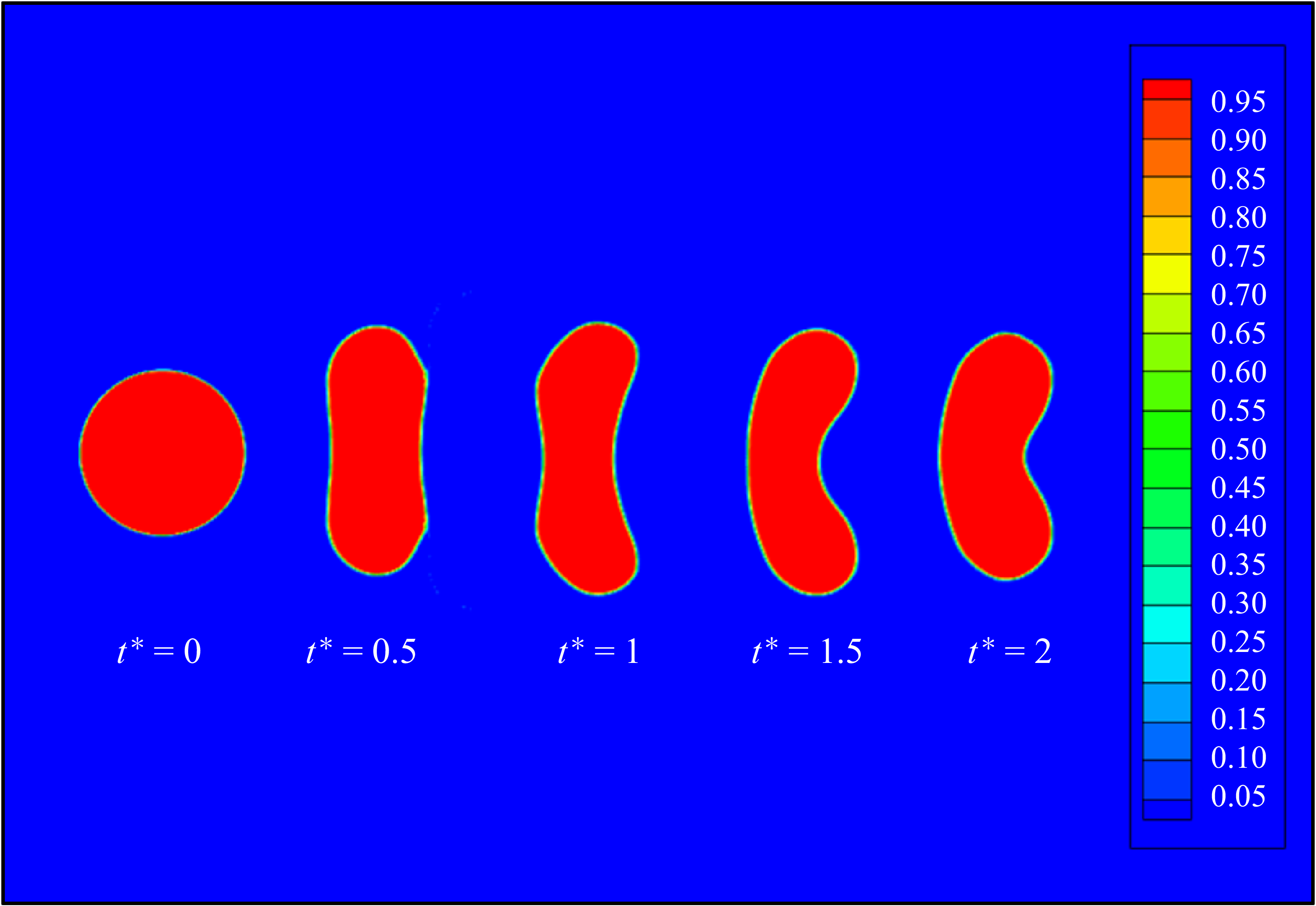
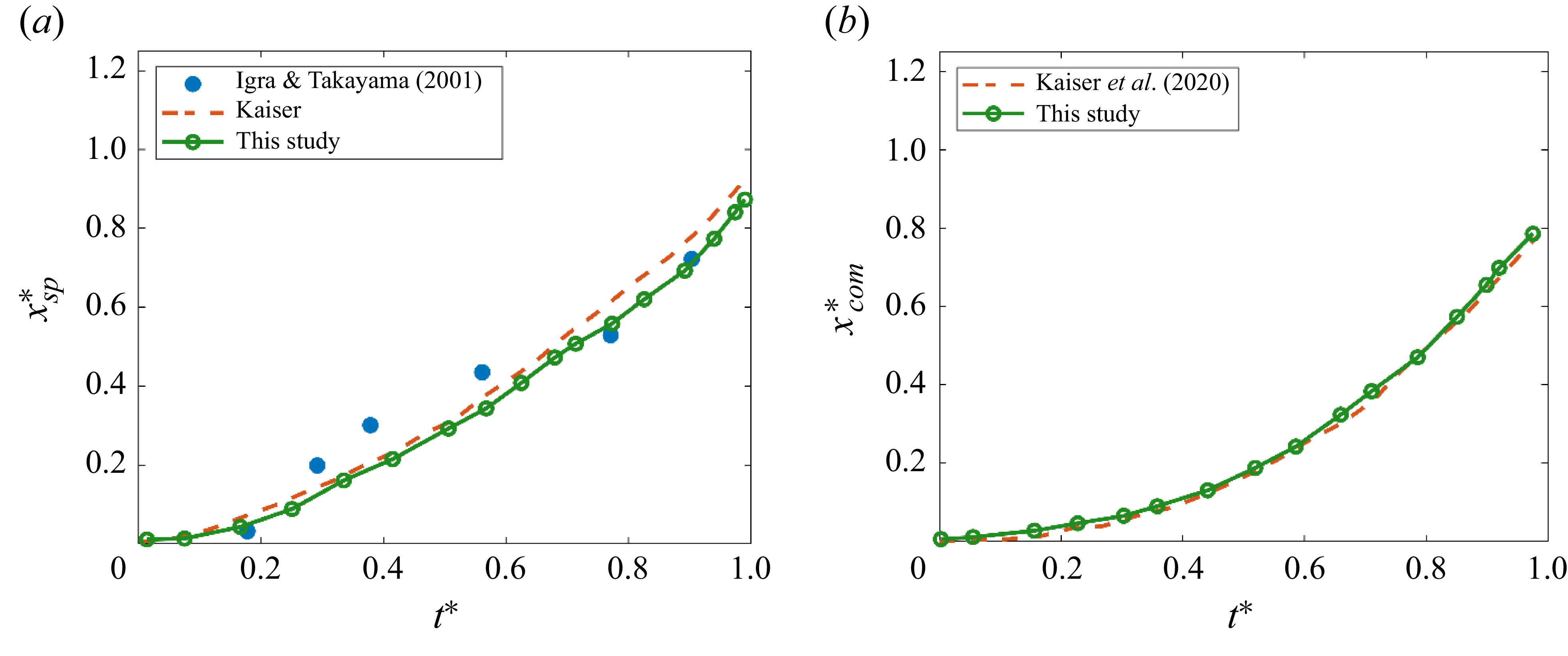
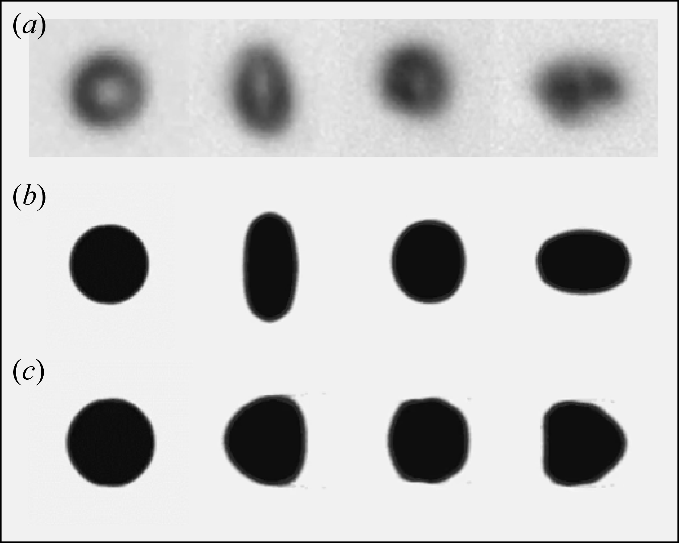
The surface tension coefficient is adopted from separate MD simulations conducted by the authors, which represents the behaviour of a nanoscale n-dodecane droplet exposed to a quiescent supercritical nitrogen environment considering different initial conditions (Jangale et al. Reference Jangale, Ehsan, Mohammad and Dorrin2024). The details of surface tension calculation using MD simulations are described in Appendix C and detailed in Jangale et al. (Reference Jangale, Ehsan, Mohammad and Dorrin2024). In this study the surface tension is calculated based on the initial conditions, i.e. background nitrogen pressure and temperature that vary among different cases, keeping the droplet temperature constant at 363 K for all cases detailed in table 1. We assume a constant surface tension, calculated based on the initial conditions, with the assumption that the droplet breakup occurs more rapidly than the transition to a fully supercritical state. This implies that the transition to the GL supercritical phase, where surface tension vanishes, is never reached during the breakup process. This is consistent with Crua et al. (Reference Crua, Julien and Lyle2017) experiments that showed droplets remained under the control of surface tension for a finite time except for very high pressures and temperatures at which the droplet transitions to a supercritical GL diffusion regime. Therefore, the simulations assume that the droplet breaks up due to the passage of the shockwave through the interface before the droplet is fully transitioned to a supercritical GL state. This assumption is further justified based on the simulation results (refer to Appendix B) that indicate the variation of density inside the droplet during the shock passage is not significant and the droplet remains in a LL state throughout the breakup process. We have shown in Appendix C that surface tension coefficient at transcritical conditions is strongly correlated with the background temperature and is not dependent on the droplet size. This behaviour justifies the use of the MD-driven surface tension coefficient in modelling microscale droplets. The surface tension effects are included in the momentum and energy equation source terms ((2.3) and (2.4)) as discussed in § 2.1. The oscillation behaviour of an initial ellipsoidal droplet (Perigaud and Saurel Reference Perigaud and Richard2005) subject to surface tension forces is used to validate the surface tension modelling procedure. The predicted droplet oscillations are validated against the global kinetic energy and theoretical period of oscillation as detailed in Appendix D. In addition, two validation cases are discussed in Appendix H: (i) water droplet–shock interaction at Mach 1.47 compared with experiments of Igra & Takayama (Reference Igra and Takayama2001) , and (ii) transcritical droplet morphology exposed to a low-speed convective flow compared with the experiments conducted by Crua et al. (Reference Crua, Julien and Lyle2017). Simulations show reasonable agreement with the experiments.

Table 1.

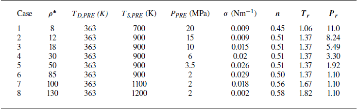
Operating conditions including n-dodecane droplet and nitrogen surrounding temperature and pressure, density ratio (ρ ^* = ${\rho _{D}}/{\rho _{\textit{POST}}}$ ), surface tension coefficient (σ), the speed of sound ratio (n), reduced pressure ( $P_{r}$ ) and reduced temperature ( $T_{r}$ ).

3.1. Non-dimensional parameters

A non-dimensional breakup time derived from the analysis of droplet–shock interaction (Hinze Reference Hinze1955; Nicholls & Ranger Reference Nicholls and Arthur1968; Guildenbecher, López-Rivera, & Sojka Reference Guildenbecher, López-Rivera and Sojka2009; Meng & Colonius Reference Meng and Tim2018), considering the droplet displacement and assuming a constant acceleration due to the drag force, is defined as

(3.2) \begin{equation} t^{*} = t\frac{u_{z,\textit{POST}}}{D_{0}}\sqrt{\frac{\rho _{\textit{POST}}}{\rho _{D}}}.\end{equation}

The instant that the shockwave first impacts the droplet interface at z = −125 µm is considered as t = 0. This non-dimensional breakup time is useful for comparing the development of droplet deformation at later times when the shockwave has fully passed through the droplet. The Weber number $(We)$ is defined based on the post-shock gas phase density ( $\rho _{\textit{POST}}$ ), post-shock velocity ( $u_{\textit{POST}}$ ), initial droplet diameter ( $D_{0}$ ) and surface tension coefficient ( $\sigma$ ) defined as ${\textit{We}} ={\rho _{\textit{POST}}u_{\textit{POST}}^{2}D_{0}}/{\sigma }.$

The engine combustion network (ECN) standard n-dodecane spray A conditions (Bruneaux et al. Reference Bruneaux, Louis-Marie, Laurent, Caspar, Jesper, Lyle and Caroline2010), commonly employed for validating computational studies that represents the transcritical conditions, serve as the primary test case. Case 4 marked in table 1 and figure 2 represents the ECN spray A conditions with the density ratio of 30 and surface tension coefficient of 0.02 N m⁻¹. Additional test cases are chosen to encompass a range of conditions outlined in table 1. The initial conditions for eight different cases considered in this study are marked in figure 2. It is noted that the critical temperature and critical pressure of pure n-dodecane are $T_{c}$ = 658.1 K and $p_{c}$ = 1.82 MPa, respectively, while the critical properties of pure nitrogen are $T_{c}$ = 126.2 K and $p_{c}$ = 3.369 MPa, respectively. The initial temperature of n-dodecane, the pressure and temperature of the surrounding nitrogen, density ratio and surface tension coefficients (calculated from MD simulations) are outlined in table 1. In this study the surface tension is calculated based on the initial conditions, which are the background nitrogen pressure and temperature, keeping the droplet temperature constant at 363 K for all cases. Furthermore, we consider a constant surface tension by assuming that the transition to the supercritical GL state at which surface tension vanishment occurs is never reached and the droplet breakup occurs faster than the transition to a fully supercritical state as discussed in § 2.3. All cases presented in table 1 represent transcritical behaviour with the initial temperature of n-dodecane (T _D,PRE ) set at 363 K, which is subcritical with respect to the nominal critical point of n-dodecane while the droplet surrounding pressure and temperature are higher than the nominal critical point of n-dodecane. The pressure varies from 2 to 20 MPa and the nitrogen temperature changes from 700 to 1200 K to represent a wide range of conditions from trans- to supercritical, representing $T_{r}={T_{S,\textit{PRE}}}/{T_{c}}$ varying from 1.06 to 1.82 and $P_{r}={P_{\textit{PRE}}}/{p_{c}}$ varying from 1.1 to 11.0, as outlined in table 1. The reduced pressure and temperature are calculated with respect to the nominal critical point of n-dodecane. In this study we focus on lower droplet temperatures that more accurately represent the initial conditions when a cold fuel is introduced into a high-pressure combustor. Accordingly, the range of nitrogen temperature and pressure considered in this study are relevant to the liquid–fuel injection experiments in high-pressure vessels (Crua, Manin, and Pickett Reference Crua, Julien and Lyle2017). The effect of higher initial droplet temperature on droplet deformation was studied in our previous work (Boyd & Jarrahbashi Reference Boyd and Jarrahbashi2021a ,Reference Boyd and Jarrahbashi b ). As table 1 outlines, a range of density ratios ( $\rho ^{*}={\rho _{D}}/{\rho _{\textit{POST}}}$ ) varying from 8 to 130 is expected by changing the surrounding temperature (T _S,PRE ) and pressure (P _PRE ), which results in changes in the surface tension coefficient ( $\sigma$ ). The details of surface tension calculation for all cases shown in table 1 is discussed in Appendix C.

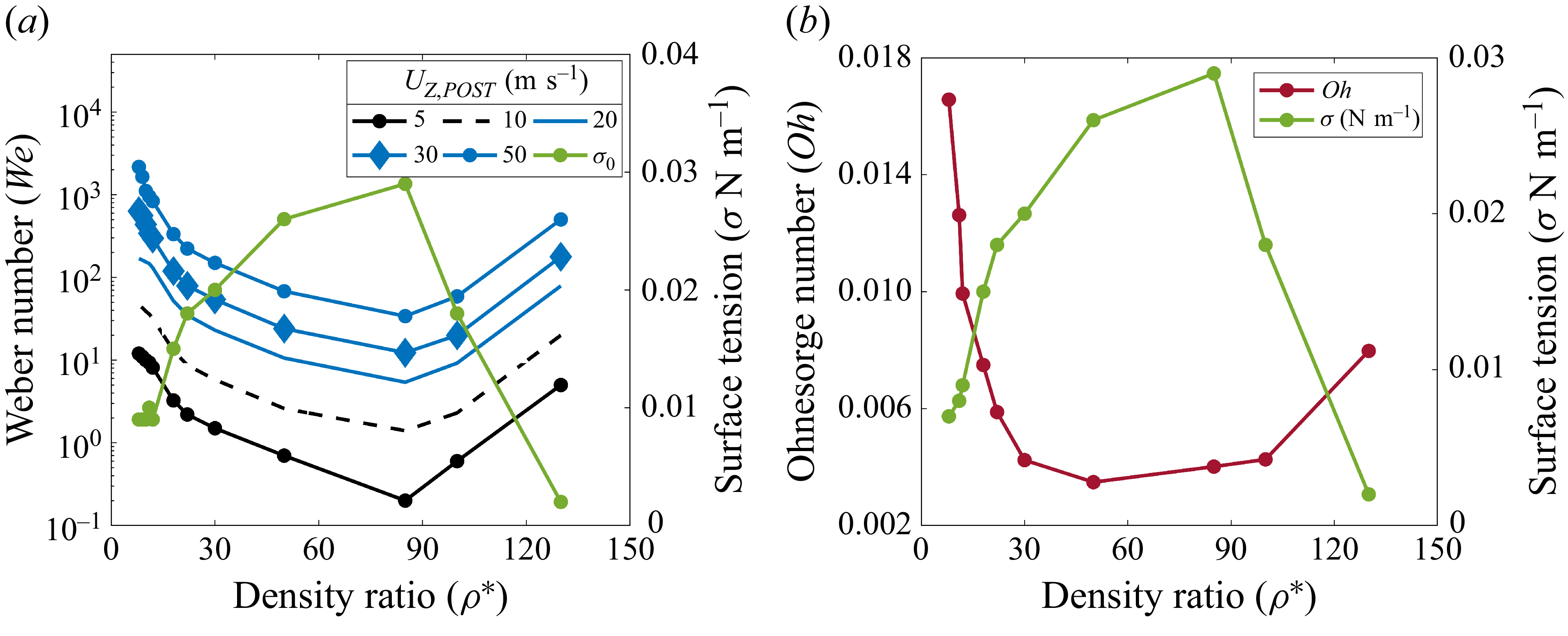
The surface tension coefficient at transcritical conditions obtained from MD simulations (Jangale et al. Reference Jangale, Ehsan, Mohammad and Dorrin2024) varies from 9 to 29 mN/m by varying the temperature from 700 to 1100 K and pressure from 2 to 20 MPa. The changes in surface tension coefficient at the transcritical condition is unique and follows the trend that the surface tension reduces drastically near the nominal critical temperature of n-dodecane. This is consistent with table 1 that shows a minimum value of 0.009 N m⁻¹ for a temperature of 700 K and 20 MPa. By fixing the temperature at 900 K and decreasing the pressure from 20 to 2 MPa, surface tension increases. By setting the pressure to 2 MPa and increasing the temperature to 1100 and 1200 K, surface tension decreases again. To better show this trend, the changes in surface tension coefficient are plotted against the density ratio that is unique for each case in table 1. Figure 3(a) illustrates the variation of the surface tension coefficient with density ratio, revealing a peak in the surface tension coefficient at a density ratio of 85, followed by a decline beyond that specific density ratio. The trend in Ohnesorge number variation with density ratio mirrors that of the Weber number, exhibiting a minimum at a density ratio of 85 as shown in figure 3(b). The Ohnesorge number is calculated along with the Weber number to reflect the range of governing non-dimensional parameters encountered in this study. The Ohnesorge number is defined as ${\textit{Oh}} =\mu _{l}/{\sqrt{\rho _{\textit{POST}}D_{0}\sigma }},$ where the droplet viscosity ( ${\mu}_{l})$ is adapted from the nominal viscosity of n-dodecane at 363 K. The outcomes presented in figure 3 suggest that variation of the surface tension coefficient with density ratio results in a broader range of Weber and Ohnesorge numbers for each flow speed. This distinctive phenomenon is specific to transcritical droplets as opposed to water droplets at subcritical conditions (Pilch & Erdman Reference Pilch and Erdman1987), where various breakup modes are less affected by density ratio while the surface tension coefficient remains constant. Thus, the breakup modes identified under subcritical conditions primarily hinge on the Weber number whilst considering exceedingly low Ohnesorge numbers (i.e. ${\textit{Oh}}$  < 0.01), whereas for transcritical droplets, the changes in density ratio simultaneously affect Weber and Ohnesorge numbers as surface tension highly varies with density ratio. It is generally accepted that inviscid simulations – those conducted without explicitly accounting for molecular viscosity – using shock- and interface-capturing schemes naturally include numerical viscosity (Garrick, Owkes, & Regele Reference Garrick, Mark and Jonathan2017; Meng & Colonius Reference Meng and Tim2018; Ma, Wu, Banuti et al. Reference Ma, Wu, Banuti and Ihme2019). In addition, studies (e.g. Lee and Reitz Reference Lee and Rolf2001) have shown that the droplet aerobreakup process across all three regimes (bag breakup, shear-stripping and catastrophic) are primarily governed by the Weber number. These studies have defied the validity of the commonly used ‘shear’ or ‘boundary-layer stripping’ theories, which attribute aerobreakup to viscous stresses and boundary layer effects at the gas–liquid interface. Instead, the breakup is driven by droplet distortion, leading to the formation of thin liquid sheets at the edges, which are stretched into ligaments by airflow and eventually break into smaller droplets. However, to ensure that neglecting viscosity and thermal conduction do not affect the identification of breakup modes, this study incorporates the viscous effects from additional test in which thermal conduction is considered (see Appendix F), showing that there is no significant impact on the droplet morphology. It is crucial to note that numerical viscosity is inherently present in all simulation results. The magnitude of this numerical viscosity is directly related to the spatial resolution of the simulation.

Figure 3.

(a) Weber number variation with density ratio for varying post-shock flow speed ( $u_{z,\textit{POST}})$ ; (b) variation of Ohnesorge number with density ratio and surface tension. The secondary plot (green line) shows the surface tension coefficient variation with density ratio.

The transcritical conditions in our study differ from conventional atmospheric aerobreakup by accounting for lower flow speeds, higher gas densities due to supercritical pressure and the fact that the surface tension is constant but varies among cases 1−8. It is noted that the surface tension coefficient is not zero, resulting in a finite Weber number, as the post-shock gas density is significantly higher than atmospheric conditions. Nonetheless, the density ratio and Weber number are instrumental in determining various aerobreakup modes, a point that will be elucidated further in this study.

Another non-dimensional parameter of interest is the ratio of the speed of sound between the droplet and the surrounding fluid defined as $n={c_{S}}/{c_{D}}$ , where c is the speed of sound and subscript D and S denote the droplet and surrounding fluid, respectively. We have shown in our earlier study that $n$ is a critical parameter that affects the shockwave dynamics interacting with transcritical droplets (Boyd & Jarrahbashi Reference Boyd and Jarrahbashi2021b ). If the speed of sound within the droplet is greater than the surrounding fluid $(n\lt 1)$ , it represents a ‘divergent’ case as the refracted shockwave within the droplet moves ahead of the incident shockwave. In contrast, if the speed of sound within the droplet is less than the surrounding fluid $(n\gt 1)$ , a ‘convergent’ case emerges as the refracted shock within the droplet lags the incident shockwave. As a result, the incident shockwave focuses on the downstream pole of the droplet leading to a noticeable jump in pressure and creating an outward axial jet in that location. As the droplet temperature is constant in this study, the speed of sound ratio varies from 0.45 to 0.58 for the cases represented in figure 2 based on the changes in the nitrogen speed of sound, and thus, all cases are associated with a divergent shock dynamics behaviour.

This study focuses on lower-Weber-number regimes and subsonic post-shock flow speeds to explore the differences in breakup modes compared with subcritical aerobreakup, which is more distinct for Weber numbers varying between 1 and 100. By altering the post-shock speed within the range between 5–50 ms⁻¹, which exposes the droplet to a subsonic flow, a diverse spectrum of Weber numbers from 0.1 to 700 is expected, which corresponds to the RTP breakup regime identified for subcritical conditions (Theofanous et al. Reference Theofanous, Ng, Chih and Mitkin2012). The density ratio is calculated based on the post-shock gas density and temperature that varies among different cases (1-8) while the droplet density at 363 K is considered constant. The changes in surface tension coefficient and post-shock density are reflected in the Weber number as depicted in figure 3(a). For a constant post-shock speed, there exists a minimum Weber number at a density ratio of 85 as the surface tension reaches its peak.