1. Introduction
Marangoni convection induced by a temperature gradient on a gas–liquid or a liquid–liquid interface is present in many natural and industrial applications on the Earth or especially in space, involving material fabrication (Ostrach Reference Ostrach1982) and crystal growth melt (Schwabe & Scharmann Reference Schwabe and Scharmann1981). An understanding of Marangoni convection is essential in practical applications and of fundamental interests for the fluid society.
Marangoni convection in an infinite thin liquid layer (Birikh Reference Birikh1966; Smith & Davis Reference Smith and Davis1983; Hu et al. Reference Hu, He, Chen and Liu2017; Kowal, Davis & Voorhees Reference Kowal, Davis and Voorhees2018; Patne, Agnon & Oron Reference Patne, Agnon and Oron2021), a rectangular cavity (Strani, Piva & Graziani Reference Strani, Piva and Graziani1983; Shieh & Yang Reference Shieh and Yang1987; Peltier & Biringen Reference Peltier and Biringen1993; Chen & Xu Reference Chen and Xu2021), a two layer system (Doi & Koster Reference Doi and Koster1993; Liu, Roux & Velarde Reference Liu, Roux and Velarde1998), a point-heating cavity (Hamed & Floryan Reference Hamed and Floryan2000; Wei, Liu & Lin Reference Wei, Liu and Lin2012), a cylindrical cavity (Kang et al. Reference Kang, Duan, Zhang, Yin, Yang and Hu2016), a liquid bridge (Kang et al. Reference Kang, Wu, Duan, Zhang, Zhou, Wang, Han, Hu and Hu2020), an annular liquid pool (Kang et al. Reference Kang, Wang, Duan, Su, He, Wu and Hu2019) and droplet systems (Zhang, Duan & Kang Reference Zhang, Duan and Kang2016; Masoudi & Kuhlmann Reference Masoudi and Kuhlmann2017; Hu, Yan & Chen Reference Hu, Yan and Chen2019) has been widely investigated using scaling analysis, asymptotic theory, numerical simulation and experiments both on the Earth and in space. Recently, Marangoni convection on a sinusoidal substrate (Yoo, Nam & Ahn Reference Yoo, Nam and Ahn2019) and a slip substrate (Kowal et al. Reference Kowal, Davis and Voorhees2018) with an oblique temperature gradient (Patne, Agnon & Oron Reference Patne, Agnon and Oron2020; Patne et al. Reference Patne, Agnon and Oron2021) or with phase change (Shmyrov et al. Reference Shmyrov, Mizev, Demin, Petukhov and Bratsun2019; Salgado Sánchez et al. Reference Salgado Sánchez, Ezquerro, Fernández and Rodríguez2020, Reference Salgado Sánchez, Ezquerro, Fernández and Rodríguez2021) has also been studied due to the increasing need in applications.
The free gas–liquid surface in a rectangular liquid pool with differentially heated sidewalls may deform because of surface tension (Sen Reference Sen1986), and the influence of deformation is qualitatively analysed by Smith & Davis (Reference Smith and Davis1983). Since experiments of Marangoni convection are mostly on the Earth, the influence of gravity has been analysed using linear stability theory, numerical simulation (Chan & Chen Reference Chan and Chen2010) and experiments through changing liquids and geometry size (Villers & Platten Reference Villers and Platten1987; Schwabe & Metzger Reference Schwabe and Metzger1989). If the Marangoni number is sufficiently large, Marangoni convection can become unstable. The instability is also determined by the Prandtl number (Smith & Davis Reference Smith and Davis1983) and the aspect ratio (Peltier & Biringen Reference Peltier and Biringen1993), and the transition route to chaos has been revealed in Earth-based experiments (Jiang, Duan & Kang Reference Jiang, Duan and Kang2017).
Although intensive studies have concerned Marangoni convection in a pool over a period of decades, dynamical evolution of Marangoni convection is unclear. That is, it has been known that when a wall is suddenly heated, a thermal boundary layer may be formed adjacent to the wall. The thickness increases with time initially, described by the scaling law of κ 1/2t 1/2 (where  $\kappa$ is thermal diffusivity and t is time, Patterson & Imberger Reference Patterson and Imberger1980), and then becomes a constant value (Cowley & Davis Reference Cowley and Davis1983). Such a thermal boundary layer may induce a temperature gradient on the gas–liquid surface, which may generate a surface tension gradient and in turn a thermocapillary force (Smith & Davis Reference Smith and Davis1983; Strani et al. Reference Strani, Piva and Graziani1983). Under such a surface tension distribution, the fluid on the surface may move from the wall for a negative temperature coefficient of surface tension (Pearson Reference Pearson1958) or to the wall for a positive temperature coefficient of surface tension (Legros, Limbourg-Fontaine & Petre Reference Legros, Limbourg-Fontaine and Petre1984; Villers & Platten Reference Villers and Platten1985). The characteristic velocity on the surface in a steady state has been described in the study by Ostrach (Reference Ostrach1982). Further, the distribution of the velocity and temperature of the surface in a steady state has also been obtained using theory, simulation and experimental methods (Birikh Reference Birikh1966; Strani et al. Reference Strani, Piva and Graziani1983; Villers & Platten Reference Villers and Platten1987, Reference Villers and Platten1992). Apart from the fluid motion on the surface, the fluid below the surface may move owing to the viscous effect. Thus, the motion of the fluid in a viscous layer and a surface layer may result in a surface flow (Smith & Davis Reference Smith and Davis1983; Kamotani, Ostrach & Pline Reference Kamotani, Ostrach and Pline1994). The viscous layer in a steady state has been described in quantity by Cowley & Davis (Reference Cowley and Davis1983). Further, Birikh (Reference Birikh1966) indicated that the thickness of the viscous layer may reach approximately H/3 (where H is the height of the pool) for a sufficiently small aspect ratio.
The fluid is convected in a surface flow away from or to the heated sidewall, which results in a pressure variance and in turn a pressure gradient. Further, the vertical boundary layer flow may form near the sidewall owing to the effect of such a pressure gradient for which a pressure gradient scale and a thickness scale in a steady state have been presented by Sen & Davis (Reference Sen and Davis1982). Additionally, a returning flow may be induced below the surface flow in a pool, which was also quantified in the study (see Sen & Davis Reference Sen and Davis1982). Here, the thickness is different for a viscous boundary layer and a thermal boundary layer near the sidewall, and has been estimated by Cowley & Davis (Reference Cowley and Davis1983) for sufficient large Prandtl numbers and Marangoni numbers in a steady state.
Although the study of a surface flow at a steady state induced by a thermocapillary force has been conducted as mentioned above, the dynamical evolution and thermal process of transient Marangoni convection are rarely investigated, except for the study by Chen & Xu (Reference Chen and Xu2021) in which a set of scaling laws only for a surface flow induced by an iso-flux wall have been obtained. That is, a complete understanding of dynamical evolution and thermal process of transient Marangoni convection remains unknown. This inspired our present work in which the dynamical evolution and thermal process of a transient Marangoni convection system involving a surface flow and a vertical flow adjacent to an isothermal sidewall of a rectangular pool are analysed, scenarios and regimes of dynamical evolution and thermal process are identified and new scaling laws under different scenarios and regimes are obtained using scaling analysis and verified based on numerical results.
In the remainder of this paper, the scaling analysis is performed in § 2, the numerical procedure is presented in § 3, selected scaling laws are verified in § 4 and conclusions are summarized in § 5.
2. Formulation and scale analysis
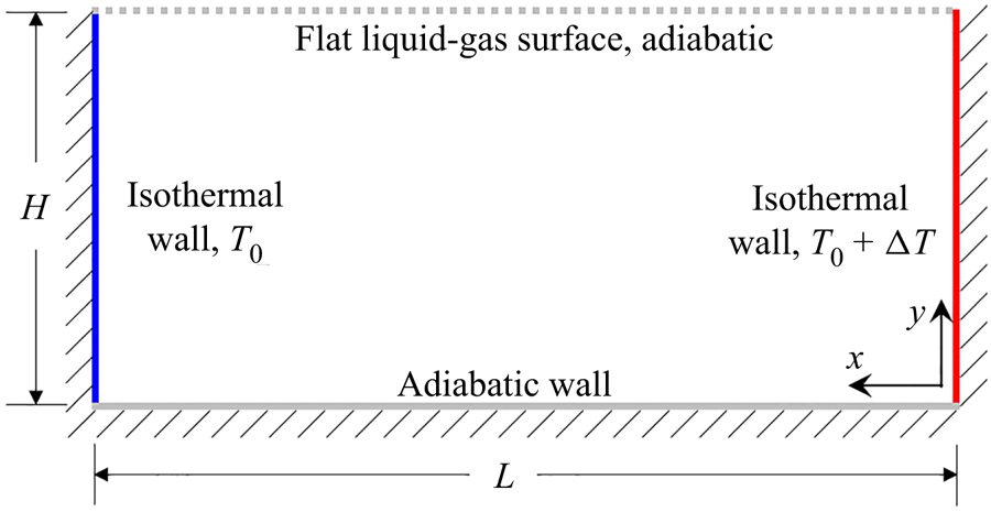
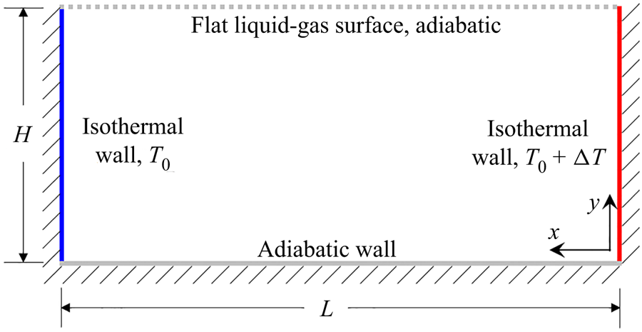
Under consideration is transient Marangoni convection under a zero-gravity condition in a two-dimensional rectangular pool. As illustrated in figure 1, the rectangular pool of length L and height H with a top open boundary subject to surface tension and three rigid no-slip boundaries contains a Newtonian fluid, which is initially isothermal (at temperature T 0) and quiescent. Here, the top boundary subject to surface tension is a gas–liquid surface. The gas–liquid surface is flat; that is, the deformation is neglected in this study since only dynamical and thermal processes are focused on. In practice, the deformation of the gas–liquid surface may be neglected for the contact angle of the liquid at the sidewall close to  ${\rm \pi}$/2 and a small Crispation number of αTΔT/α (where αT is a temperature coefficient for surface tension, αT = ∂α/∂T, α is the surface tension of liquid, T is temperature and ΔT is the temperature difference between two sidewalls, also see Strani et al. Reference Strani, Piva and Graziani1983). The gas–liquid surface is assumed to be adiabatic; that is, the heat exchange across the surface is neglected since the temperature difference between the gas and the liquid on the two sides of the surface is small and dynamical evolution of transient Marangoni convection is our focus (also see Strani et al. Reference Strani, Piva and Graziani1983; Villers & Platten Reference Villers and Platten1992). The right-hand sidewall is suddenly heated to the temperature T 0 + ΔT at t = 0 and remains at this temperature thereafter. The condition of sudden heating was usually adopted in previous experimental studies for which hot water was used to suddenly and quickly flush the wall (also see Wang, Xu & Zhai Reference Wang, Xu and Zhai2018). Additionally, the condition of ramp heating was also used in previous studies with different dynamical evolutions, as illustrated in previous studies by Jiang, Nie & Xu (Reference Jiang, Nie and Xu2019) and Jiang et al. (Reference Jiang, Nie, Zhao, Carmeliet and Xu2021). Further, the left-hand sidewall is maintained at temperature T 0, and the bottom boundary is assumed to be adiabatic.
Schematic of a rectangular pool with isothermal sidewalls.
The two-dimensional (2-D) Navier–Stokes and energy equations may describe such a transient Marangoni convection (Pimputkar & Ostrach Reference Pimputkar and Ostrach1980; Shieh & Yang Reference Shieh and Yang1987):
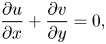 \begin{gather}\frac{{\partial u}}{{\partial x}} + \frac{{\partial v}}{{\partial y}} = 0,\end{gather}
 \begin{gather}\frac{{\partial u}}{{\partial t}} + u\frac{{\partial u}}{{\partial x}} + v\frac{{\partial u}}{{\partial y}} ={-} \frac{1}{\rho }\frac{{\partial p}}{{\partial x}} + \nu \left( {\frac{{{\partial^2}u}}{{\partial {x^2}}} + \frac{{{\partial^2}u}}{{\partial {y^2}}}} \right) + {F_\alpha },\end{gather}
 \begin{gather}\frac{{\partial v}}{{\partial t}} + u\frac{{\partial v}}{{\partial x}} + v\frac{{\partial v}}{{\partial y}} ={-} \frac{1}{\rho }\frac{{\partial p}}{{\partial y}} + \nu \left( {\frac{{{\partial^2}v}}{{\partial {x^2}}} + \frac{{{\partial^2}v}}{{\partial {y^2}}}} \right),\end{gather}
 \begin{gather}\frac{{\partial T}}{{\partial t}} + u\frac{{\partial T}}{{\partial x}} + v\frac{{\partial T}}{{\partial y}} = \kappa \left( {\frac{{{\partial^2}T}}{{\partial {x^2}}} + \frac{{{\partial^2}T}}{{\partial {y^2}}}} \right),\end{gather}
where, u and v denote velocity components in the x and y directions, x and y are the horizontal and vertical coordinates, t is time, ρ is density, p is pressure, ν is kinematic viscosity, κ is thermal diffusivity and Fα is a thermocapillary force by non-uniform surface tension (Popinet Reference Popinet2018). The studies in e.g. Tryggvason, Scardovelli & Zaleski (Reference Tryggvason, Scardovelli and Zaleski2011) and Popinet (Reference Popinet2018) indicate that the thermocapillary force on a flat gas–liquid surface can be given by
 \begin{equation}{F_{\alpha}} =
\frac{1}{\rho }{\alpha _T}\frac{{\partial T}}{{\partial
x}}\delta ,\quad \int_{H -\varepsilon }^H {\delta
\,\textrm{d}y = 1} ,\end{equation}
where δ is a Dirac function at the surface and ε denotes the thickness of the gas–liquid surface layer. Previous studies indicate that the thickness ε is approximately tens of nanometres (Tryggvason et al. Reference Tryggvason, Scardovelli and Zaleski2011) with the fluctuation of a few Angstroms (de Gennes, Brochard Wyart & Quéré Reference de Gennes, Brochard Wyart and Quéré2013); that is, it is very thin. Note that the gas–liquid surface layer in which the thermocapillary force is dominant is located between H–ε and H, as described in (2.5a,b).
Dimensional analysis shows that transient Marangoni convection here is determined by the four governing parameters: the Marangoni number, the Prandtl number and the aspect ratios, which are given by
 \begin{equation}Ma = \frac{{|{\alpha _T}|\Delta TL}}{{\rho \nu \kappa }},\quad Pr = \frac{\nu }{\kappa },\quad A = \frac{H}{L},\quad {A_\varepsilon } = \frac{\varepsilon }{L}.\end{equation}
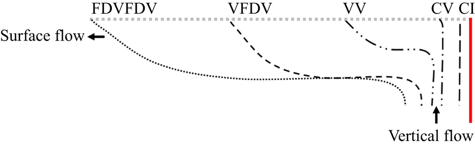
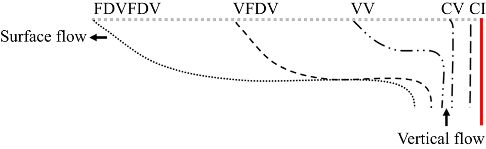
In what follows, we will consider transient Marangoni convection in a rectangular pool for which Ma > 1, Pr > 1 and A < 1, and analyse (2.1)–(2.4) in order to understand the dynamical evolution and thermal process of transient Marangoni convection induced by an isothermal sidewall. The development of transient Marangoni convection may be classified into different stages under different dynamical regimes, as illustrated in figure 2.
Schematic of transient Marangoni convection. Dotted and dashed lines represent different stages of surface flow under different dynamical regimes, which involves CI, CV, VV, VFDV and FDVFDV stages (also see table 1).
2.1. Surface flow
2.1.1. Dynamical origin
It may be expected that when the sidewall is suddenly heated, a thermal boundary layer forms adjacent to and along the heated sidewall owing to conduction. Further, heat transfer in the fluid adjacent to the heated sidewall is described by (2.4) in which the unsteady term is approximately O(ΔT/t), the convection term O(vΔT/H) and the conduction term  $O(\kappa \Delta T/\delta _T^2)$ since δT < H, where δT denotes the thickness of the thermal boundary layer. Clearly, the convection term is negligible in comparison with the conduction term for a sufficiently small time. Therefore, a balance between conduction and unsteady terms may yield a thickness scale,
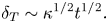 \begin{equation}{\delta _T}\sim {\kappa ^{1/2}}{t^{1/2}}.\end{equation}
It is clear that the thickness of the thermal boundary layer increases with t 1/2; that is, the distribution of the temperature of the fluid varies in the x direction and is dependent on time.
Such a temperature difference in the x direction may result in a thermocapillary force on the gas–liquid surface, as described in (2.5a,b). Further, the thermocapillary force may drive away the fluid on the surface from the sidewall. In addition, a viscous layer may form below owing to the viscous effect induced by the motion of the fluid on the surface. The motion of the fluid in the surface layer and the viscous layer results in a surface flow.
2.1.2. Dynamical evolution
To analyse the dynamical evolution of the surface flow, the viscous layer is discussed first. Equation (2.2) may be used to analyse the flow in the viscous layer. If the thickness of the viscous layer is denoted by Δν, in (2.2), the unsteady term is approximately O(u/t), the advection term O(u 2/L) and the viscous term  $O(\nu u/\varDelta _n^2)$, but the thermocapillary force term may be neglected outside the surface layer. Additionally, the advection term can also be negligible in comparison with the unsteady term for a sufficiently small time. Therefore, the balance between unsteady and viscous terms in a small time may yield,
 \begin{equation}{\varDelta _\nu }\sim P{r^{1/2}}{\kappa ^{1/2}}{t^{1/2}}.\end{equation}
Note that the unsteady term and the advection term become of the same order when t ~ L/u.
The value of Δν may increase with time and reach the maximum value H, the height of the pool. Inserting H into (2.8), we may obtain a time scale at which the pool may be occupied by a viscous layer,
 \begin{equation}{t_\nu }\sim \frac{{{A^2}{L^2}}}{{Pr\kappa }}.\end{equation}
The fluid in the surface layer and the viscous layer moves from the sidewall owing to thermocapillary and viscous effects, which in turn results in a surface flow. Such a surface flow may be analysed using (2.2). Clearly, the advection term may be negligible in comparison with the unsteady term for a sufficiently small time, as illustrated in (2.7) and (2.8). In fact, the advection term may also be negligible even for a large time since Pr > 1 in (2.2). The gas–liquid surface in which the thermocapillary force is dominant is between H–ε and H. Accordingly, the integral of (2.2) in the y direction from H–ε to H (that is, on the surface) can be given by
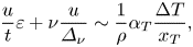 \begin{equation}\frac{u}{t}\varepsilon + \nu \frac{u}{{{\varDelta _\nu }}}\sim \frac{1}{\rho }{\alpha _T}\frac{{\Delta T}}{{{x_T}}},\end{equation}
where, xT is a length scale in which the temperature significantly varies on the surface. Note that the second term in the left side of (2.10) is an approximate integral of the second term in the right side of (2.2) for which ν∂u/∂y is approximately νu/Δν at y = H–ε but zero at y = H (the density and viscosity of the gas are negligible compared with those of the liquid, and the continuity of stress on the gas–liquid surface is considered, see Batchlor Reference Batchlor2000). Here, Δν denotes the thickness of the surface flow because ε is very small. Additionally, xT could be δT, ut or even L in different stages, since the heated fluid in the surface flow moves away from the sidewall.
Based on (2.7) and (2.8), the ratio of the unsteady term to the viscous term is O(ε/Pr 1/2κ 1/2t 1/2). This means that the viscous term is negligible in comparison with the unsteady term for a sufficiently small time in which xT may be described by δT. That is, the surface flow is initially governed by a balance between the thermocapillary term and the unsteady term, yielding a velocity scale,
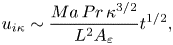 \begin{equation}{u_{i\kappa }}\sim \frac{{Ma\,Pr\,{\kappa ^{3/2}}}}{{{L^2}{A_\varepsilon }}}{t^{1/2}},\end{equation}
where the subscript iκ means that the surface flow moves under the balance between the unsteady term and the conduction induced thermocapillary term.
Based on (2.8), the balance between the unsteady term and the viscous term in (2.10) may yield a time scale,
 \begin{equation}{t_{i\nu }}\sim \frac{{A_\varepsilon ^2{L^2}}}{{Pr\kappa }}.\end{equation}
Equation (2.12) means that, as time goes on, the heated fluid is convected away from the sidewall and thus the length scale xT changes from δT to ut when ut > δT. Further, based on (2.11), the time for uiκt ~ δT may be described by
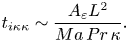 \begin{equation}{t_{i\kappa \kappa }}\sim \frac{{{A_\varepsilon }{L^2}}}{{Ma\,Pr\,\kappa }}.\end{equation}
Clearly, tiν < tiκκ for  $Ma < A_\varepsilon ^{ - 1}$, but tiν > tiκκ for
 $Ma > A_\varepsilon ^{ - 1}$. As has been mentioned above, ε is approximately tens of nanometres; that is, usually Aε < 10−5. Since Marangoni convection may be oscillatory or even chaotic for Ma > 105 (see Villers & Platten Reference Villers and Platten1992; Jiang et al. Reference Jiang, Duan and Kang2017; Salgado Sánchez et al. Reference Salgado Sánchez, Ezquerro, Fernández and Rodríguez2021), the case of
 $Ma < A_\varepsilon ^{ - 1}$ is considered in this study.
In the case of  $Ma < A_\varepsilon ^{ - 1}$, when t > tiν, the unsteady term in (2.10) is negligible; that is, the balance is mainly between viscous and thermocapillary terms. This balance yields a velocity scale of the surface flow,
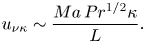 \begin{equation}{u_{\nu \kappa }}\sim \frac{{Ma\,P{r^{1/2}}\kappa }}{L}.\end{equation}
Further, when uνκt ~ δT, we obtain such a time scale,
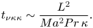 \begin{equation}{t_{\nu \kappa \kappa }}\sim \frac{{{L^2}}}{{M{a^2}Pr\,\kappa }}.\end{equation}
According to (2.9) and (2.15), we have tνκκ < tν for Ma > A −1 but tνκκ > tν for Ma < A −1. Since the thermocapillary convection is usually very weak for Ma < A −1 in comparison with that for Ma > A −1 (also see Villers & Platten Reference Villers and Platten1992), the thermocapillary convection for Ma > A −1 is studied in the following analysis. When t > tνκκ, the thermocapillary term in (2.10) is O(αTΔT/ρut). The balance between the thermocapillary term and the viscous term  $O(\nu u/\varDelta _n^2)$ may yield a velocity scale,
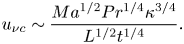 \begin{equation}{u_{\nu c}}\sim \frac{{M{a^{1/2}}P{r^{1/4}}{\kappa ^{3/4}}}}{{{L^{1/2}}{t^{1/4}}}}.\end{equation}
Using (2.16), the time scale at which the surface flow arrives the other sidewall (penetrates through the whole pool, L) can be given by
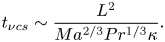 \begin{equation}{t_{\nu cs}}\sim \frac{{{L^2}}}{{M{a^{2/3}}P{r^{1/3}}\kappa }}.\end{equation}
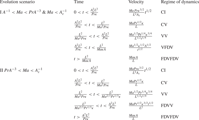
Comparing tν in (2.9) with tνcs in (2.17), it is found that tν < tνcs for Ma < PrA −3 but tν > tνcs for Ma > PrA −3. Accordingly, the evolution scenario of the surface flow may be described as follows:
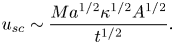
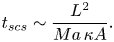
(a) For A −1 < Ma < PrA −3, tν is smaller than tνcs, indicating that Δν becomes H before the surface flow arrives the other sidewall (at which uνct ~ L). Therefore, when t > tν, the viscous term in (2.10) is O(νu/H 2) and xT ~ ut for the thermocapillary force, yielding a velocity scale of the surface flow,
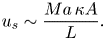
(2.18)Thus, the time scale at which xT becomes L may be expressed as \begin{equation}{u_{sc}}\sim \frac{{M{a^{1/2}}{\kappa ^{1/2}}{A^{1/2}}}}{{{t^{1/2}}}}.\end{equation}(2.19)when t > tscs, the thermocapillary force in (2.10) is\begin{equation}{t_{scs}}\sim \frac{{{L^2}}}{{Ma\,\kappa A}}.\end{equation}$O({\alpha _T}\Delta T/\rho L)$, and the velocity scale can be given by
(2.20)\begin{equation}{u_s}\sim \frac{{Ma\,\kappa A}}{L}.\end{equation}
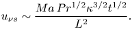
(b) For Ma > PrA −3, tν is larger than tνcs, implying that xT is O(L) before Δν reaches H. Therefore, when t > tνcs, the thermocapillary term in (2.10) is
$O({\alpha _T}\Delta T/\rho L)$ and the viscous term is $O(\nu u/\varDelta _n^2)$, yielding a new velocity scale of the surface flow
(2.21)\begin{equation}{u_{\nu s}}\sim \frac{{Ma\,P{r^{1/2}}{\kappa ^{3/2}}{t^{1/2}}}}{{{L^2}}}.\end{equation}



Additionally, when t > tν, the viscous term in (2.10) becomes the order of O(νu/H 2), and thus the velocity scale at a steady state is the same as that in (2.20).
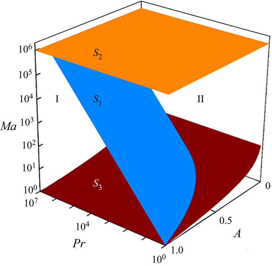
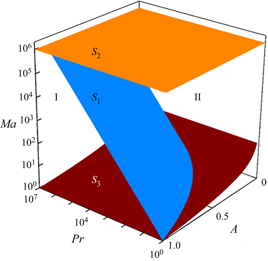
In summary, the evolution scenario (ES) of the surface flow involves ES I for  $Ma < A_\varepsilon ^{ - 1}$ and A −1 < Ma < PrA −3 and ES II for
 $Pr{A^{ - 3}} < Ma < A_\varepsilon ^{ - 1}$. ESs and velocity scales of the surface flow are also illustrated in table 1. Further, ESs are shown in the Ma–Pr–A space in figure 3. Note that, as described above, only the scenarios for
 $Ma < A_\varepsilon ^{ - 1}$ for which the flow is usually laminar are considered.
ESs of surface flow. Surface S 1: Ma = PrA −3,  ${S_2}:Ma = A_\varepsilon ^{ - 1}$, S 3: Ma = A −1. The value of Aε is assumed to be 10−6. Since the scenarios for Ma < A −1 and
 $Ma > A_\varepsilon ^{ - 1}$ are beyond the consideration of this work, the space for Ma > A −1 and
 $Ma > A_\varepsilon ^{ - 1}$ is not shown.
Surface flow under different regimes in different ESs.
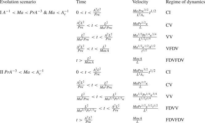
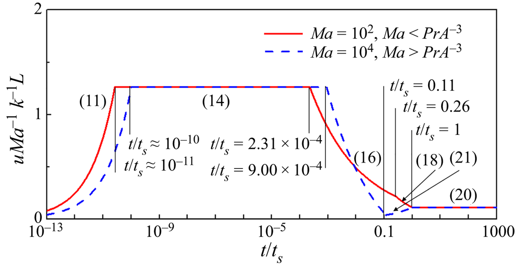
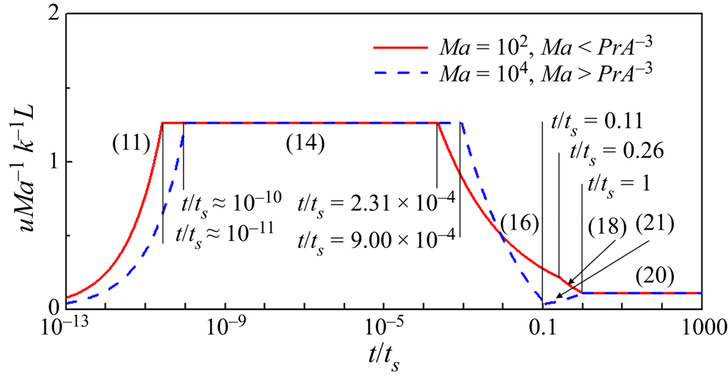
The development of the surface flow may be classified into different stages and is shown in figure 4. Clearly, as time goes, the velocity usually increases in the first stage scaled by (2.11) in both ESs I and II, then remains a constant value in the second stage scaled by (2.14) in both ESs I and II, decreases in the third stage scaled by (2.16) in both ESs I and II, decreases further in the fourth stage scaled by (2.18) in ES I but slightly increases scaled by (2.21) in ES II and finally remains a constant value again in the fifth stage scaled by (2.20) in both ESs I and II. That is, different stages of the surface flow are dominated under conduction induced thermocapillary inertial (CI), conduction induced thermocapillary viscous (CV), convection induced thermocapillary viscous (VV), convection induced thermocapillary fully developed viscous (VFDV) and fully developed convection induced thermocapillary fully developed viscous (FDVFDV) regimes in ES I (which are also illustrated in figure 2) but under CI, CV, VV, fully developed convection induced thermocapillary viscous (FDVV) and FDVFDV regimes in ES II, respectively, as listed in table 1.
Velocity of surface flow for Pr = 14.3 and A = 1/3 in ESs I and II. Here, ts denotes the time scale for surface flow to reach steady state, which is ts = tscs, given by (2.19) in ES I for A −1 < Ma < PrA −3 and  $Ma < A_\varepsilon ^{ - 1}$, but ts = tν, given by (2.9) in ES II for
 $Pr{A^{ - 3}} < Ma < A_\varepsilon ^{ - 1}$.
2.2. Vertical flow
2.2.1. Dynamical origin
As illustrated in figure 2, the surface flow convects the fluid from the sidewall, which may result in a pressure drop in the horizontal direction near the sidewall. Thus, a balance between the thermocapillary term and the pressure gradient term may be achieved in the horizontal momentum equation (2.2). Further, integrating equation (2.2) in y direction from H–Δν to H, we may obtain
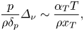 \begin{equation}\frac{p}{{\rho {\delta _p}}}{\varDelta _\nu }\sim \frac{{{\alpha _T}T}}{{\rho {x_T}}},\end{equation}
where δp is a thickness of a vertical flow adjacent to the sidewall, which will be estimated in what follows. Such a pressure drop may also induce a vertical pressure gradient and in turn drive a vertical flow adjacent to the sidewall.
As described by (2.22), the vertical flow adjacent to the sidewall may be induced by a thermocapillary induced pressure gradient. Further, the penetration distance of the vertical flow is also vt for t < H/v and H for t ≥ H/v. Since the surface flow originates from the vertical flow, the volumetric flow rate for the vertical flow is equal to that for the surface flow
 \begin{equation}Q\sim u{\varDelta _\nu }\sim v{\delta _p}.\end{equation}
As described in § 2.1 and illustrated in figure 4, the velocity may be different for the surface flow under different regimes, involving uiκ, uνκ, uνc, usc (or uνs) and us in sequence. Accordingly, the dynamical evolution of the vertical flow will also be discussed in sequence. Note that the ESs of the vertical flow induced by the surface flow only in ES I (in the case for  $Ma < A_\varepsilon ^{ - 1}$ and A −1 < Ma < PrA −3) are analysed in this section for a brief discussion; additionally, those in ES II (in the case for
 $Pr\,{A^{ - 3}} < Ma < A_\varepsilon ^{ - 1}$) are presented in Appendix A.
2.2.2. Dynamical evolution
Since the vertical flow is driven by the surface flow induced pressure gradient adjacent to the sidewall, the dynamical evolution of the vertical flow will be discussed in CI, CV, VV, VFDV and FDVFDV stages in sequence in the following section (also see table 1).
(a) CI stage
In this stage, the surface flow is dominated under the CI regime. The transition time from this stage to CV stage described by (2.12) is very small. In fact, the transition time is smaller than 10−9 s for most liquids. In this stage, 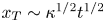 ${x_T}\sim {\kappa ^{1/2}}{t^{1/2}}$. The penetration distance of the vertical flow is O(vt). Using (2.22), the vertical pressure gradient over vt is given by
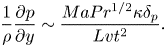 \begin{equation}\frac{1}{\rho }\frac{{\partial p}}{{\partial y}}\sim \frac{{MaP{r^{1/2}}\kappa {\delta _p}}}{{Lv{t^2}}}.\end{equation}
Further, the volumetric flow rate for the vertical flow supplying the surface flow may be written as
 \begin{equation}{Q_{i\kappa }}\sim {u_{i\kappa }}{\varDelta _\nu }\sim \frac{{MaP{r^{3/2}}{\kappa ^2}}}{{{A_\varepsilon }{L^2}}}t.\end{equation}
Additionally, the inertial term is approximately O(v/t) and the viscous term is  $O(\nu v/\delta _p^2)$ in the vertical momentum equation (2.3). Using (2.24) and (2.25), the balance between the vertical pressure gradient term and the inertial term in (2.3) yields a velocity scale and a thickness scale under a thermocapillary inertial regime
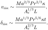 \begin{equation}\begin{array}{c} {v_{ii\kappa }}\sim \dfrac{{M{a^{2/3}}P{r^{2/3}}\kappa }}{{A_\varepsilon ^{1/3}L}},\\ {\delta _{ii\kappa }}\sim \dfrac{{M{a^{1/3}}P{r^{5/6}}\kappa t}}{{A_\varepsilon ^{2/3}L}}. \end{array}\end{equation}
On the other hand, using (2.24) and (2.25), the balance between the vertical pressure gradient term and the viscous term yields a velocity scale and a thickness scale under a thermocapillary viscous regime
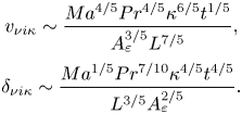 \begin{equation}\begin{array}{c} {v_{\nu i\kappa }}\sim \dfrac{{M{a^{4/5}}P{r^{4/5}}{\kappa ^{6/5}}{t^{1/5}}}}{{A_\varepsilon ^{3/5}{L^{7/5}}}},\\ {\delta _{\nu i\kappa }}\sim \dfrac{{M{a^{1/5}}P{r^{7/10}}{\kappa ^{4/5}}{t^{4/5}}}}{{{L^{3/5}}A_\varepsilon ^{2/5}}}. \end{array}\end{equation}
For either (2.26) or (2.27), a time scale at which the inertial term is equivalent to the viscous term may be expressed as
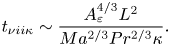 \begin{equation}{t_{\nu ii\kappa }}\sim \frac{{A_\varepsilon ^{4/3}{L^2}}}{{M{a^{2/3}}P{r^{2/3}}\kappa }}.\end{equation}
Clearly, the vertical flow rises adjacent to the sidewall under a thermocapillary viscous regime when t < tνiiκ but under a thermocapillary inertial regime when t > tνiiκ. The ratio of tνiiκ to tiν (also see (2.12)) is  ${t_{\nu ii\kappa }}/{t_{i\nu }}\sim P{r^{1/3}}/(M{a^{2/3}}A_\varepsilon ^{2/3})$. Since Pr > 1 and
 $Ma < A_\varepsilon ^{ - 1}$ in the case of ES I, tνiiκ > tiν. This implies that the balance between the vertical pressure gradient and the viscous term dominates the vertical flow in CI stage.
If time is sufficiently large, the penetration distance of the vertical flow becomes vt ~ H. Using (2.27), the time scale is given by
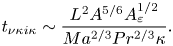 \begin{equation}{t_{\nu \kappa i\kappa }}\sim \frac{{{L^2}{A^{5/6}}A_\varepsilon ^{1/2}}}{{M{a^{2/3}}P{r^{2/3}}\kappa }}.\end{equation}
According to (2.12),  ${t_{\nu \kappa i\kappa }}/{t_{i\nu }}\sim P{r^{1/3}}/(M{a^{2/3}}A_\varepsilon ^{3/2})$. Since Ma < PrA −3 in the case of ES I, tνκiκ > tiν. This means that the penetration distance of the vertical flow in the case of ES I is vt in CI stage.
Consider the vertical thermal boundary layer adjacent to the sidewall. According to the energy equation (2.4), the ratio of the unsteady term O(ΔT/t) to the convection term O(vΔT/H) is O(H/v/t). Since the time scale tνκiκ is larger than tiν, O(H/v/t) is larger than unity. This means that the vertical thermal boundary layer adjacent to the sidewall evolves under the balance between unsteady and conduction terms in CI stage.
(b) CV stage
As time increases, the thickness of the surface flow becomes larger, and 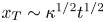 ${x_T}\sim {\kappa ^{1/2}}{t^{1/2}}$ in the CV stage. The penetration distance of the vertical flow is initially O(vt). Using (2.22), the vertical pressure gradient over vt is given by (2.24). Further, a volumetric flow rate for a vertical flow may be given by
 \begin{equation}{Q_{\nu \kappa }}\sim {u_{\nu \kappa }}{\varDelta _\nu }\sim \frac{{Ma\,Pr\,{\kappa ^{3/2}}{t^{1/2}}}}{L}.\end{equation}
Repeating the discussion of (2.26) and (2.27), based on (2.22) and (2.30), we may obtain the velocity scale and the thickness scale under a thermocapillary inertial regime
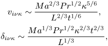 \begin{equation}\begin{array}{c} {v_{i\nu \kappa }}\sim \dfrac{{M{a^{2/3}}P{r^{1/2}}{\kappa ^{5/6}}}}{{{L^{2/3}}{t^{1/6}}}},\\ {\delta _{i\nu \kappa }}\sim \dfrac{{M{a^{1/3}}P{r^{1/2}}{\kappa ^{2/3}}{t^{2/3}}}}{{{L^{1/3}}}}, \end{array}\end{equation}
and under a thermocapillary viscous regime
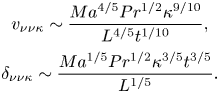 \begin{equation}\begin{array}{c} {v_{\nu \nu \kappa }}\sim \dfrac{{M{a^{4/5}}P{r^{1/2}}{\kappa ^{9/10}}}}{{{L^{4/5}}{t^{1/10}}}},\\ {\delta _{\nu \nu \kappa }}\sim \dfrac{{M{a^{1/5}}P{r^{1/2}}{\kappa ^{3/5}}{t^{3/5}}}}{{{L^{1/5}}}}. \end{array}\end{equation}
If the inertial term becomes equivalent to the viscous term, based on either (2.31) or (2.32), we further obtain a time scale
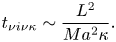 \begin{equation}{t_{\nu i\nu \kappa }}\sim \frac{{{L^2}}}{{M{a^2}\kappa }}.\end{equation}
Clearly, the vertical flow is dominated under a thermocapillary viscous regime when t < tνiνκ in which the inertial term is smaller than the viscous term but under a thermocapillary inertial regime when t > tνiνκ in which the inertial term is larger than the viscous term. Note that tνiνκ > tνκκ for Pr > 1 based on (2.15). This implies that the balance between the vertical pressure gradient and the viscous term dominates the vertical flow in CV stage.
Consider the vertical thermal boundary layer adjacent to the sidewall. We have vt ~ H if the convection term O(vT/H) and the unsteady term O(T/t) are equivalent in the energy equation (2.4). Using (2.32), the balance between convection and unsteady terms yields a time scale
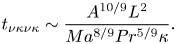 \begin{equation}{t_{\nu \kappa \nu \kappa }}\sim \frac{{{A^{10/9}}{L^2}}}{{M{a^{8/9}}P{r^{5/9}}\kappa }}.\end{equation}
Here, tνκνκ is also a time scale for the penetration distance vt to grow to H. According to (2.15), tνκνκ > tνκκ for Ma > A −1 and Pr > 1. This implies that the vertical thermal boundary layer is dominated by the balance between conduction and unsteady terms, and the penetration distance of the vertical flow is vt in the CV stage.
(c) VV stage
In this stage, xT ~ ut. Additionally, as described above, the penetration distance of the vertical flow is vt for t < H/v and H for t ≥ H/v. That is, (2.22) may be expressed as
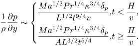 \begin{equation}\frac{1}{\rho }\frac{{\partial p}}{{\partial y}}\sim \left\{ {\begin{array}{*{20}{@{}l}} {\dfrac{{M{a^{1/2}}P{r^{1/4}}{\kappa^{3/4}}{\delta_p}}}{{{L^{1/2}}{t^{9/4}}v}},}&{t < \dfrac{H}{v},}\\ {\dfrac{{M{a^{1/2}}P{r^{1/4}}{\kappa^{3/4}}{\delta_p}}}{{A{L^{3/2}}{t^{5/4}}}},}&{t \ge \dfrac{H}{v}.} \end{array}} \right.\end{equation}
Further, the volumetric flow rate for the surface flow is equal to that for the vertical flow, defined as
 \begin{equation}{Q_{\nu c}}\sim {u_{\nu c}}{\varDelta _\nu }\sim \frac{{M{a^{1/2}}P{r^{3/4}}{\kappa ^{5/4}}{t^{1/4}}}}{{{L^{1/2}}}}.\end{equation}
Repeating the discussion of (2.26) and (2.27), based on (2.35) and (2.36), we have the velocity scale and the thickness scale under a thermocapillary inertial regime
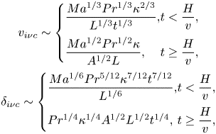 \begin{equation}\begin{array}{c} {v_{i\nu c}}\sim \left\{ {\begin{array}{*{20}{@{}l}} {\dfrac{{M{a^{1/3}}P{r^{1/3}}{\kappa^{2/3}}}}{{{L^{1/3}}{t^{1/3}}}},}&{t < \dfrac{H}{v},}\\ {\dfrac{{M{a^{1/2}}P{r^{1/2}}\kappa }}{{{A^{1/2}}L}},}&{t \ge \dfrac{H}{v},} \end{array}} \right.\\ {\delta _{i\nu c}}\sim \left\{ {\begin{array}{*{20}{@{}l}} {\dfrac{{M{a^{1/6}}P{r^{5/12}}{\kappa^{7/12}}{t^{7/12}}}}{{{L^{1/6}}}},}&{t < \dfrac{H}{v},}\\ {P{r^{1/4}}{\kappa^{1/4}}{A^{1/2}}{L^{1/2}}{t^{1/4}},}&{t \ge \dfrac{H}{v},} \end{array}} \right. \end{array}\end{equation}
and under a thermocapillary viscous regime
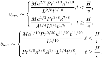 \begin{equation}\begin{array}{c} {v_{\nu \nu c}}\sim \left\{ {\begin{array}{*{20}{@{}l}} {\dfrac{{M{a^{2/5}}P{r^{3/10}}{\kappa^{7/10}}}}{{{L^{2/5}}{t^{3/10}}}},}&{t < \dfrac{H}{v},}\\ {\dfrac{{M{a^{1/2}}P{r^{3/8}}{\kappa^{7/8}}}}{{{A^{1/4}}{L^{3/4}}{t^{1/8}}}},}&{t \ge \dfrac{H}{v},} \end{array}} \right.\\ {\delta _{\nu \nu c}}\sim \left\{ {\begin{array}{*{20}{@{}l}} {\dfrac{{M{a^{1/10}}P{r^{9/20}}{\kappa^{11/20}}{t^{11/20}}}}{{{L^{{1 / {10}}}}}},}&{t < \dfrac{H}{v},}\\ {P{r^{3/8}}{\kappa^{3/8}}{A^{1/4}}{L^{1/4}}{t^{3/8}},}&{t \ge \dfrac{H}{v}.} \end{array}} \right. \end{array}\end{equation}
When the inertial term becomes equivalent to the viscous term, based on either (2.37) or (2.38), we further obtain a time scale
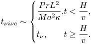 \begin{equation}{t_{\nu i\nu c}}\sim \left\{ {\begin{array}{*{20}{@{}l}} {\dfrac{{Pr{L^2}}}{{M{a^2}\kappa }},}&{t < \dfrac{H}{v},}\\ {{t_\nu },}&{t \ge \dfrac{H}{v}.} \end{array}} \right.\end{equation}
It is clear that tνiνc/tνκκ > 1, and  ${t_{\nu i\nu c}}/{t_\nu }\sim {(Pr/Ma\,A)^2}$ when t < H/v or tνiνc/tν ~ 1 when t ≥ H/v. This means that the vertical flow moves firstly under a thermocapillary viscous regime in the VV stage.
Consider the vertical thermal boundary layer adjacent to the sidewall. Similar to the CV stage, we have vt ~ H if the convection term and the unsteady term in the energy equation (2.4) are equivalent. Using (2.37) and (2.38), the time scale in the balance between convection and unsteady terms may be expressed as, respectively,
 \begin{equation}{t_{\nu \kappa \nu c}}\sim \frac{{{L^2}{A^{10/7}}}}{{M{a^{4/7}}P{r^{3/7}}\kappa }},\quad {t_{i\kappa \nu c}}\sim \frac{{{L^2}{A^{3/2}}}}{{M{a^{1/2}}P{r^{1/2}}\kappa }}.\end{equation}
That is, the time scale at which the functioning distance of the vertical pressure gradient is H may be described by tνκνc under a thermocapillary viscous regime but by tiκνc under a thermocapillary inertial regime. Further, based on (2.9) and (2.39), we may have  ${t_{\nu k\nu c}}/{t_{\nu i\nu c}}\sim {(MaA/Pr)^{10/7}}$ and
 ${t_{i\kappa \nu c}}/{t_{\nu i\nu c}}\sim {(MaA/Pr)^{3/2}}$ (when the penetration distance is vt). In the case of
 ${A^{ - 1}} < Ma < Pr\,{A^{ - 1}}({t_\nu } < {t_{\nu \kappa \nu c}} < {t_{\nu i\nu c}})$, the vertical flow may be dominated by the thermocapillary viscous regime, and heat transfer is under the balance between unsteady and conduction terms in the VV stage. Further, in the case of Ma > PrA −1 (tνκκ < tνiνc < tiκνc < tν), the vertical flow may be dominated by the thermocapillary viscous regime under the balance between unsteady and conduction terms when tνκκ < t < tνiνc, by the thermocapillary inertial regime under the balance between unsteady and conduction terms when tνiνc < t < tiκνc but by a thermocapillary inertial regime under the balance between convection and conduction terms when tiκνc < t < tν. According to (2.37), a balance between conduction and convection terms in the energy equation (2.4) may yield a thickness scale when tiκνc < t < tν in the case for Ma > PrA −1
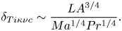 \begin{equation}{\delta _{Ti\kappa \nu c}}\sim \frac{{L{A^{3/4}}}}{{M{a^{1/4}}P{r^{1/4}}}}.\end{equation}
(d) VFDV)stage
In this stage, Δν ~ H and xT ~ ut. The analysis above shows that the penetration distance of the vertical flow is vt for t < H/v and H for t ≥ H/v in the case of A −1 < Ma < PrA −1, but only H in the case of Ma > PrA −1 in VFDV stage. Thus, (2.22) is expressed as
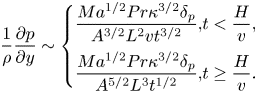 \begin{equation}\frac{1}{\rho }\frac{{\partial p}}{{\partial y}}\sim \left\{ {\begin{array}{*{20}{@{}l}} {\dfrac{{M{a^{1/2}}Pr{\kappa^{3/2}}{\delta_p}}}{{{A^{3/2}}{L^2}v{t^{3/2}}}},}&{t < \dfrac{H}{v},}\\ {\dfrac{{M{a^{1/2}}Pr{\kappa^{3/2}}{\delta_p}}}{{{A^{5/2}}{L^3}{t^{1/2}}}},}&{t \ge \dfrac{H}{v}.} \end{array}} \right.\end{equation}
Further, the volumetric flow rate for a vertical flow supplying a surface flow can be given by
 \begin{equation}{Q_{sc}}\sim {u_{sc}}H\sim \frac{{M{a^{1/2}}{\kappa ^{1/2}}{A^{3/2}}L}}{{{t^{1/2}}}}.\end{equation}
Repeating the analysis of (2.26) and (2.27), based on (2.42) and (2.43), we obtain the velocity scale and the thickness scale under a thermocapillary inertial regime
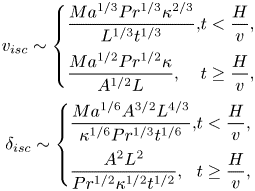 \begin{equation}\begin{array}{c} {v_{isc}}\sim \left\{ {\begin{array}{*{20}{@{}l}} {\dfrac{{M{a^{1/3}}P{r^{1/3}}{\kappa^{2/3}}}}{{{L^{1/3}}{t^{1/3}}}},}&{t < \dfrac{H}{v},}\\ {\dfrac{{M{a^{1/2}}P{r^{1/2}}\kappa }}{{{A^{1/2}}L}},}&{t \ge \dfrac{H}{v},} \end{array}} \right.\\ {\delta _{isc}}\sim \left\{ {\begin{array}{*{20}{@{}l}} {\dfrac{{M{a^{1/6}}{A^{3/2}}{L^{4/3}}}}{{{\kappa^{1/6}}P{r^{1/3}}{t^{1/6}}}},}&{t < \dfrac{H}{v},}\\ {\dfrac{{{A^2}{L^2}}}{{P{r^{1/2}}{\kappa^{1/2}}{t^{1/2}}}},}&{t \ge \dfrac{H}{v},} \end{array}} \right. \end{array}\end{equation}
and under a thermocapillary viscous regime
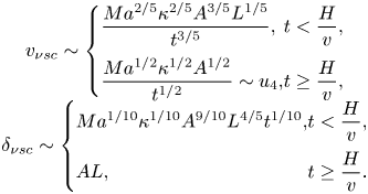 \begin{equation}\begin{array}{c} {v_{\nu sc}}\sim \left\{ {\begin{array}{*{20}{@{}l}} {\dfrac{{M{a^{2/5}}{\kappa^{2/5}}{A^{3/5}}{L^{1/5}}}}{{{t^{3/5}}}},}&{t < \dfrac{H}{v},}\\ {\dfrac{{M{a^{1/2}}{\kappa^{1/2}}{A^{1/2}}}}{{{t^{1/2}}}}\sim {u_4},}&{t \ge \dfrac{H}{v},} \end{array}} \right.\\ {\delta _{\nu sc}}\sim \left\{ {\begin{array}{*{20}{@{}l}} {M{a^{1/10}}{\kappa^{1/10}}{A^{9/10}}{L^{4/5}}{t^{1/10}},}&{t < \dfrac{H}{v},}\\ {AL,}&{t \ge \dfrac{H}{v}.} \end{array}} \right. \end{array}\end{equation}
Similar to the discussion of (2.33), letting the inertial term be equivalent to the viscous term, we obtain a time scale based on equation either (2.44) or (2.45)
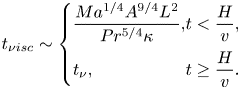 \begin{equation}{t_{\nu isc}}\sim \left\{ {\begin{array}{*{20}{@{}l}} {\dfrac{{M{a^{1/4}}{A^{9/4}}{L^2}}}{{P{r^{5/4}}\kappa }},}&{t < \dfrac{H}{v},}\\ {{t_\nu },}&{t \ge \dfrac{H}{v}.} \end{array}} \right.\end{equation}
It is clear that tνisc < tν for Ma < PrA −1 and tνisc ~ tν for Ma > PrA −1. This implies that the vertical flow can be dominated by a thermocapillary viscous regime in the VFDV stage.
Consider the vertical thermal boundary layer adjacent to the sidewall. The unsteady term and the convection term are O(T/t) and O(vT/H) in the energy equation (2.4), respectively. Thus, a time scale for which the two terms are equivalent may be expressed as
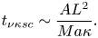 \begin{equation}{t_{\nu \kappa sc}}\sim \frac{{A{L^2}}}{{Ma\kappa }}.\end{equation}
Based on (2.9), we further have tνκsc/tν ~ Pr/MaA and  ${t_{\nu \kappa sc}}/{t_{scs}}\sim {A^2} < 1$. Therefore, in the case of A −1 < Ma < PrA −1, heat transfer of the vertical thermal boundary layer is under the balance between unsteady and conduction terms when tν < t < tνκsc but under the balance between convection and conduction terms when tνκsc < t < tscs. In the case of Ma > PrA −1, heat transfer of the vertical thermal boundary layer is under the balance between convection and conduction terms. Note that the vertical flow is dominated by a thermocapillary viscous regime in the VFDV stage in both cases. According to (2.45), the balance between the convection and conduction terms in (2.4) yields a thickness scale of the vertical thermal boundary layer when tνκsc < t < tscs in the case of A −1 < Ma < PrA −1 and in the whole VFDV stage in the case of Ma > PrA −1
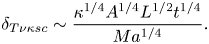 \begin{equation}{\delta _{T\nu \kappa sc}}\sim \frac{{{\kappa ^{1/4}}{A^{1/4}}{L^{1/2}}{t^{1/4}}}}{{M{a^{1/4}}}}.\end{equation}
(e) FDVFDV stage
In this stage, Δν ~ H and xT ~ L. According to the analysis in the VFDV stage, the penetration distance of the vertical flow is H. Equation (2.22) may be written as
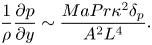 \begin{equation}\frac{1}{\rho }\frac{{\partial p}}{{\partial y}}\sim \frac{{MaPr{\kappa ^2}{\delta _p}}}{{{A^2}{L^4}}}.\end{equation}
The volumetric flow rate for a vertical flow supplying a surface flow is given by
 \begin{equation}{Q_{ss}}\sim {u_s}{\varDelta _\nu }\sim Ma\kappa {A^2}.\end{equation}
Repeating the analysis of (2.26) and (2.27), based on (2.49) and (2.50), we may obtain the velocity scale and the thickness scale under a thermocapillary inertial regime
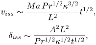 \begin{equation}\begin{array}{c} {v_{iss}}\sim \dfrac{{Ma\,P{r^{1/2}}{\kappa ^{3/2}}}}{{{L^2}}}{t^{1/2}},\\ {\delta _{iss}}\sim \dfrac{{{A^2}{L^2}}}{{P{r^{1/2}}{\kappa ^{1/2}}{t^{1/2}}}}, \end{array}\end{equation}
and under a thermocapillary viscous regime
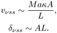 \begin{equation}\begin{array}{c} {v_{\nu ss}}\sim \dfrac{{Ma\kappa A}}{L},\\ {\delta _{\nu ss}}\sim AL. \end{array}\end{equation}
Similar to the discussion of (2.33), based on equation either (2.51) or (2.52), letting the inertial term be equivalent to the viscous term, we have a time scale tνiss ~ tν. That is, the inertial term is smaller than the viscous term when t > tνiss. Since  ${t_{\nu iss}}/{t_{scs}}\sim Ma{A^3}/Pr < 1$ in ES I, the vertical flow can be dominated by the thermocapillary viscous regime in the FDVFDV stage.
Consider the vertical thermal boundary layer adjacent to the sidewall. Unsteady and convection terms are O(T/t) and O(vT/H) in the energy equation (2.4), respectively. A time scale at which unsteady and convection terms become equivalent may be expressed as
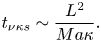 \begin{equation}{t_{\nu \kappa s}}\sim \frac{{{L^2}}}{{Ma\kappa }}.\end{equation}
It is clear that tνκs/tscs ~ A < 1. This implies that heat transfer of the vertical thermal boundary layer is under the balance between convection and conduction terms in the FDVFDV stage. Using (2.52), the balance between convection and conduction terms may further yield a thickness of the vertical thermal boundary layer in the FDVFDV stage,
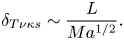 \begin{equation}{\delta _{T\nu \kappa s}}\sim \frac{L}{{M{a^{1/2}}}}.\end{equation}
If the thermal boundary layer is distinct, the thickness must be smaller than H; thus, we may obtain a criterion
 \begin{equation}Ma > \frac{1}{{{A^2}}}.\end{equation}
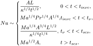
The heat transfer through the sidewall can be scaled by  $O(\lambda \Delta T/{\delta _T})$, where λ is thermal conductivity. Further, we may normalize the heat flux using λΔT/H and obtain the Nusselt number (Nu) for Ma < PrA −1 based on (2.7), (2.48) and (2.54), respectively,
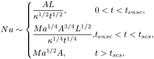 \begin{equation}Nu\sim \left\{
{\begin{array}{*{20}{@{}l}}
{\dfrac{{AL}}{{{\kappa^{1/2}}{t^{1/2}}}},}&{0 < t <
{t_{\nu \kappa sc}},}\\
{\dfrac{{M{a^{1/4}}{A^{3/4}}{L^{1/2}}}}{{{\kappa^{1/4}}{t^{1/4}}}},}&{{t_{\nu
\kappa sc}} < t < {t_{scs}},}\\ {M{a^{1/2}}A,}&{t >
{t_{scs}},} \end{array}} \right. \end{equation}
and for Ma > PrA −1 based on (2.7), (2.41), (2.48) and (2.54), respectively,
The heat transfer through the sidewall can be scaled by  $O(\lambda \Delta T/{\delta _T})$, where λ is thermal conductivity. Further, we may normalize the heat flux using λΔT/H and obtain the Nusselt number (Nu) for Ma < PrA −1 based on (2.7), (2.48) and (2.54), respectively,
 \begin{equation}
Nu\sim \left\{ {\begin{array}{*{20}{@{}l}}
{\dfrac{{AL}}{{{\kappa^{1/2}}{t^{1/2}}}},}&{0 < t <
{t_{i\kappa \nu c}},}\\
{M{a^{1/4}}P{r^{1/4}}{A^{1/4}},}&{{t_{i\kappa \nu c}} < t
< {t_\nu },}\\
{\dfrac{{M{a^{1/4}}{A^{3/4}}{L^{1/2}}}}{{{\kappa^{1/4}}{t^{1/4}}}},}&{{t_\nu
} < t < {t_{scs}},}\\ {M{a^{1/2}}A,}&{t > {t_{scs}}.}
\end{array}}
\right.\end{equation}
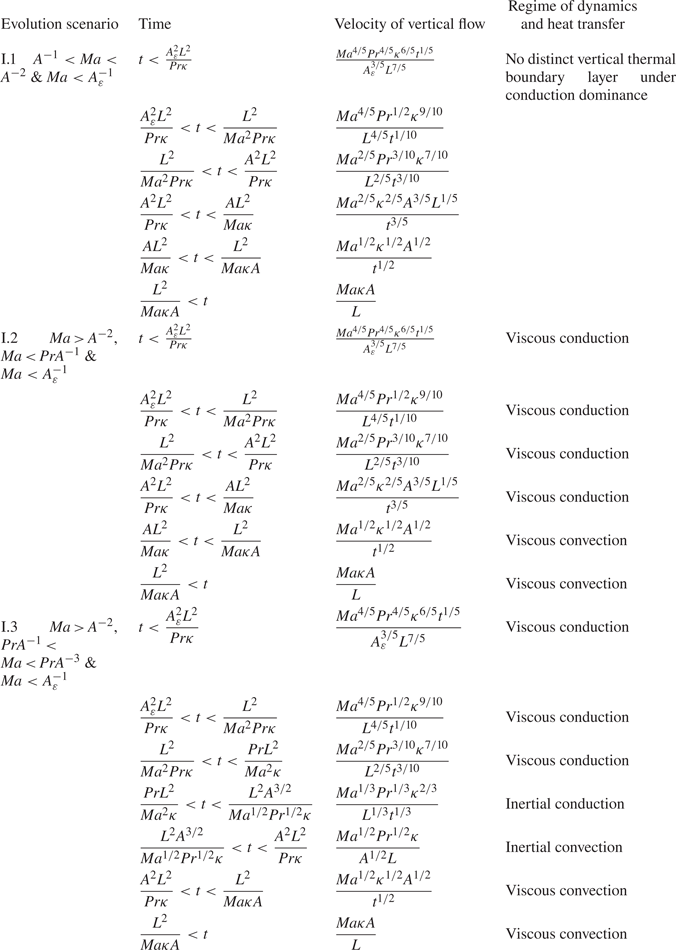
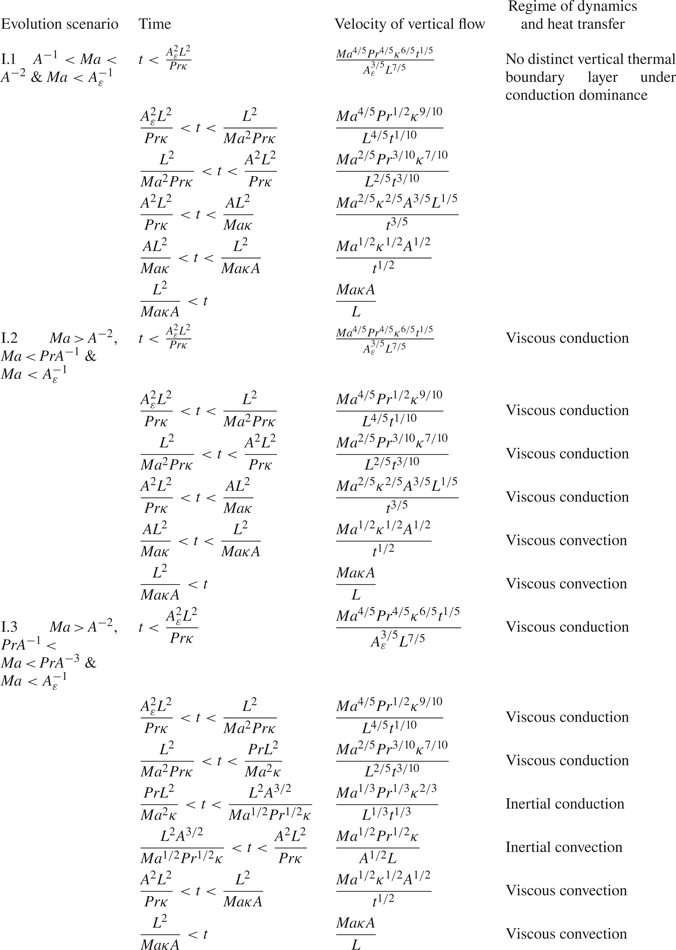
All ESs and regimes for the vertical flow are also summarized in table 2.
3. Numerical method
To understand transient Marangoni convection and to validate the scaling laws in § 2, we performed 2-D numerical simulations. The non-dimensional format was adopted in the following section. The governing Navier–Stokes and energy equations were normalized based on  $x/{x^\ast }$,
 $y/{y^\ast }$,
 $\delta /{\delta ^\ast }$ and
 $\varepsilon /{\varepsilon ^\ast }\sim L$,
 $t/{t^\ast }\sim {L^2}/(Ma\,\kappa )$,
 ${T^\ast }\sim (T - {T_0})/\Delta T$,
 $u/{u^\ast }$ and
 $v/{v^\ast }\sim Ma\,\kappa /L$ and
 $p/{p^\ast }\sim \rho M{a^2}{\kappa ^2}/{L^2}$ (Peltier & Biringen Reference Peltier and Biringen1993), and are given by
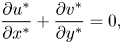 \begin{gather}\frac{{\partial {u^ \ast }}}{{\partial {x^ \ast }}} + \frac{{\partial {v^ \ast }}}{{\partial {y^ \ast }}} = 0,\end{gather}
 \begin{gather}\frac{{\partial {u^ \ast }}}{{\partial {t^ \ast }}} + {u^ \ast }\frac{{\partial {u^ \ast }}}{{\partial {x^ \ast }}} + {v^ \ast }\frac{{\partial {u^ \ast }}}{{\partial {y^ \ast }}} ={-} \frac{{\partial {p^ \ast }}}{{\partial {x^ \ast }}} + \frac{{Pr}}{{Ma}}\left( {\frac{{{\partial^2}{u^ \ast }}}{{\partial {x^ \ast }^2}} + \frac{{{\partial^2}{u^ \ast }}}{{\partial {y^ \ast }^2}}} \right), \end{gather}
 \begin{gather}\frac{{\partial {v^ \ast }}}{{\partial {t^ \ast }}} + {u^ \ast }\frac{{\partial {v^ \ast }}}{{\partial {x^ \ast }}} + {v^ \ast }\frac{{\partial {v^ \ast }}}{{\partial {y^ \ast }}} ={-} \frac{{\partial {p^ \ast }}}{{\partial {y^ \ast }}} + \frac{{Pr}}{{Ma}}\left( {\frac{{{\partial^2}{v^ \ast }}}{{\partial {x^ \ast }^2}} + \frac{{{\partial^2}{v^ \ast }}}{{\partial {y^ \ast }^2}}} \right),\end{gather}
 \begin{gather}\frac{{\partial {T^ \ast }}}{{\partial {t^ \ast }}} + {u^ \ast }\frac{{\partial {T^ \ast }}}{{\partial {x^ \ast }}} + {v^ \ast }\frac{{\partial {T^ \ast }}}{{\partial {y^ \ast }}} = \frac{1}{{Ma}}\left( {\frac{{{\partial^2}{T^ \ast }}}{{\partial {x^ \ast }^2}} + \frac{{{\partial^2}{T^ \ast }}}{{\partial {y^ \ast }^2}}} \right).\end{gather}
Vertical flow under different regimes in ES I. Here, viscous denotes that the vertical flow is under the balance between the thermocapillary induced pressure gradient term and the viscous term, and inertial denotes that the vertical flow is under the balance between the thermocapillary induced pressure gradient term and the inertial term.
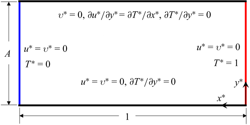
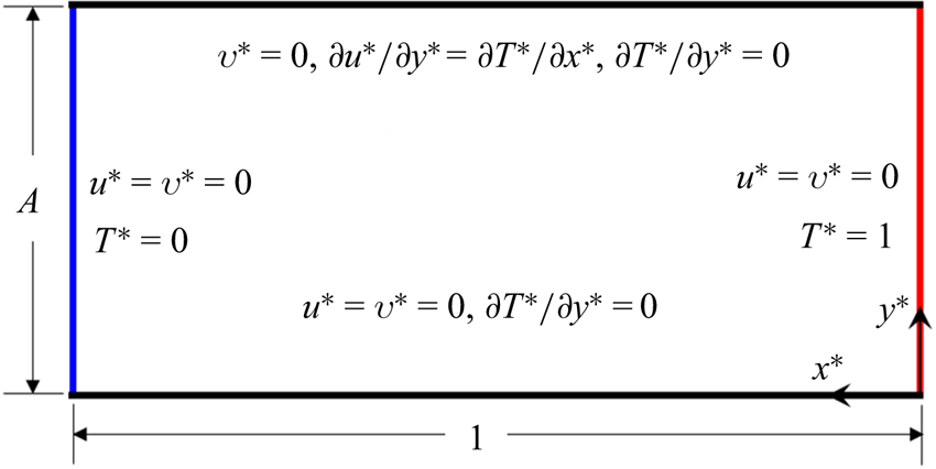
The computational domain with boundary conditions is illustrated in figure 5. Here, the thermocapillary force was presented using a boundary condition as the study by Villers & Platten (Reference Villers and Platten1990), which is expressed as
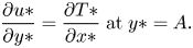 \begin{equation}\frac{{\partial u\ast }}{{\partial y\ast }} = \frac{{\partial T\ast }}{{\partial x\ast }}\;\textrm{at}\;y\ast = A.\end{equation}
That is, a Marangoni stress was imposed on the top boundary. The other boundaries were no slip. The temperature was unity at the right boundary but zero at the left boundary at t ≥ 0; upper and bottom boundaries were adiabatic. The fluid was initially quiescent and isothermal at a temperature equal to zero. The study by Popinet (Reference Popinet2018) indicates that the present numerical procedure can describe Marangoni convection in the rectangular pool with such a Marangoni stress and flat surface.
Schematic of computational domain with boundary conditions.
We solved (3.1)–(3.4) adopting a finite volume method with a semi-implicit method for pressure linked equations (SIMPLE) algorithm. The diffusion term was discretized by the second-order central difference scheme, the advection term by the quadratic upstream interpolation for convective kinematics (QUICK) scheme and the time term by the second-order implicit scheme. The numerical procedure was successfully applied for the simulation of Marangoni convection in the pool (Zeng et al. Reference Zeng, Mizuseki, Simamura, Fukuda, Higashino and Kawazoe2001; Chen & Xu Reference Chen and Xu2021) and of buoyancy convection (e.g. Xu, Patterson & Lei Reference Xu, Patterson and Lei2009).
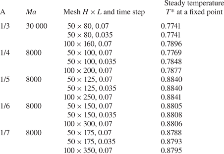
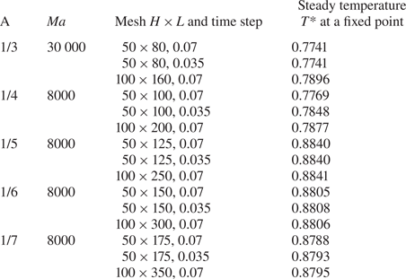
The dependency test of the mesh was carried out for aspect ratios of 1/3, 1/4, 1/5, 1/6 and 1/7. Non-uniform grids with finer near boundaries and which were coarser inside the core were built adopting ANSYS/ICEM. The Marangoni number used for each aspect ratio is the largest one in this study. Table 3 presents the test results in which the temperature difference is less than 2 % using different meshes for every A. Additionally, the dependency test of time step was also conducted, and the test results are listed in table 3. Based on the test results in table 3, a mesh of 50 × 80 and a time step of 0.07 were adopted for A = 1/3, a mesh of 50 × 100 and a time step of 0.07 for A = 1/4, a mesh of 50 × 125 and a time step of 0.07 for A = 1/5 and a mesh of 50 × 150 and a time step of 0.07 for A = 1/6 and a mesh of 50 × 175 and a time step of 0.07 for A = 1/7. Clearly, the test has proven that numerical accuracy is guaranteed. Further, the examination of the numerical results shows that, since time step and grids in proximity to the sidewall are sufficiently small, the mismatch between initial and boundary conditions may be smoothly solved using such a finite volume method (also see Jiang et al. Reference Jiang, Nie and Xu2019, Reference Jiang, Nie, Zhao, Carmeliet and Xu2021).
Dependency test of mesh and time step.
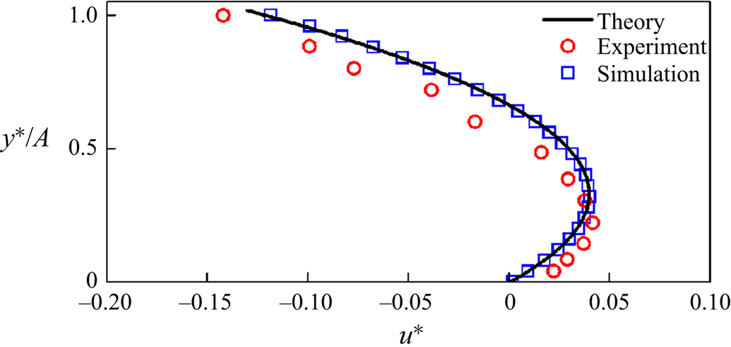
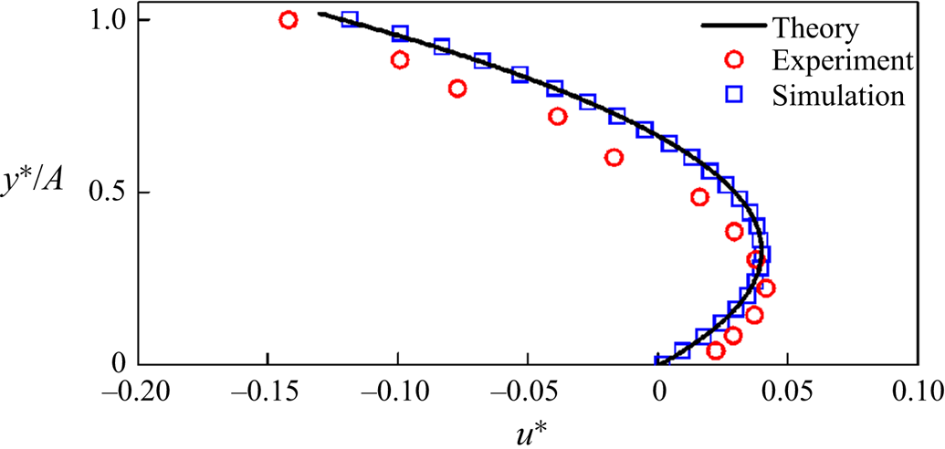
For further validation, we also compared the present results with the experiment in Villers & Platten (Reference Villers and Platten1992) and the analytical result in Smith & Davis (Reference Smith and Davis1983), which are shown in figure 6 for Ma = 7600, A = 0.083 and Pr = 4.24. Clearly, the results are coincident with the analytical result but with the experiment with small differences. That is, the numerical results can describe Marangoni convection in the pool. The small differences with the experiment may be attributed to the fact that the numerical results are two-dimensional and the upper boundary is assumed to be adiabatic.
Velocity profiles at x* = 0.5 in the case of Ma = 7600, A = 0.083 and Pr = 4.24 where the experiment is from Villers & Platten (Reference Villers and Platten1992), and the theoretical solution is from Smith & Davis (Reference Smith and Davis1983).
4. Flow structure and validation
We have performed 2-D numerical simulations for Marangoni numbers from 101 to 104, Prandtl numbers from 14.3 to 285.7 and aspect ratios from 0.17 to 0.33 in order to cover different ESs. Numerical results are used to characterize transient Marangoni convection under different regimes and to verify selected scaling laws obtained in § 2.
4.1. Flow structure
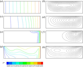
Figure 7 shows typical flows in different scenarios. The flow at a steady stage of 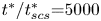 ${t^\ast }/t_{scs}^\ast{=} 5000$ for A −1 < Ma < A −2 in ES I.1 (also see table 2) is shown in figure 7(a). It is clear that there does not exist a distinct boundary layer. The isotherms are approximately parallel with nearly the same interval between any two neighbouring isotherms. This implies that the convective flow is weak and conduction dominates heat transfer. Additionally, there exists one large circulation, approximately symmetrical about the vertical centre line, as illustrated by the streamlines in figure 7(b). Figure 7(c) shows isotherms at
 ${t^\ast }/t_{scs}^\ast{=} 0.6$ under a viscous conduction regime in ES I.2 (see table 2). Clearly, the interval between neighbouring isotherms is not uniform and obviously decreases near the heated sidewall. Further, the isotherms become slightly contorted. This is because a stronger convective flow occurs for which a surface flow moves from the right sidewall but the back flow moves to the right sidewall, as shown in figure 7(d). The circulation is not symmetrical and closer to the heated sidewall owing to the stronger convective flow adjacent to the heated sidewall.
Isotherms (left) and streamlines (right) for A = 1/3 and Pr = 14.3 in different ESs. The intervals of isotherms and streamlines are 0.1 from 0.05 to 0.95. (a,b) At 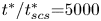 ${t^\ast }/t_{scs}^\ast{=} 5000$ for Ma = 5 in ES I.1. (c,d) At
 ${t^\ast }/t_{scs}^\ast{=} 0.6$ for Ma = 40 in ES I.2. (e,f) At
 ${t^\ast }/t_{scs}^\ast{=} 0.2$ for Ma = 3000 in ES I.3. (g,h) At
 ${t^\ast }/t_\nu ^\ast{=} 0.4$ for Ma = 30 000 in ES II.
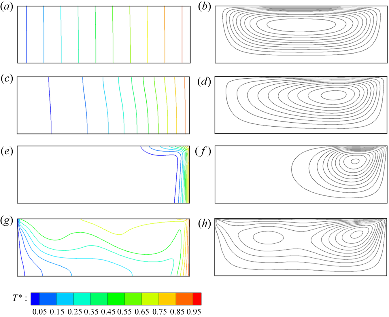
It is expected that the convective flow becomes stronger with the increase of the Marangoni number. Figure 7(e) shows isotherms at  ${t^\ast }/t_{scs}^\ast{=} 0.2$ under an inertial conduction regime in ES I.3. The vertical thermal boundary layer becomes distinct along the sidewall. In fact, the more heat may be convected away from the downstream end of the sidewall, as illustrated by the streamlines in figure 7(f). The circulation becomes smaller owing to the stronger convective flow.
Figure 7(g) shows further isotherms at  ${t^\ast }/t_\nu ^\ast{=} 0.4$ for Ma = 30 000 in ES II. Clearly, the convective flow becomes much stronger and in turn oscillations can result because the Marangoni number is larger, as illustrated by the isotherms in figure 7(g) and streamlines with two circulations in figure 7(h). Note that the thermal boundary layer forms only along with the heated sidewall owing to the effect of heat transfer, as shown in figures 7(e) and 7(g).
4.2. Verification of scaling laws
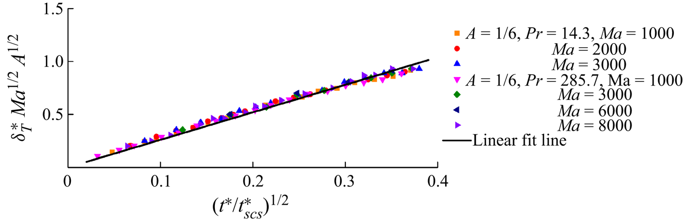
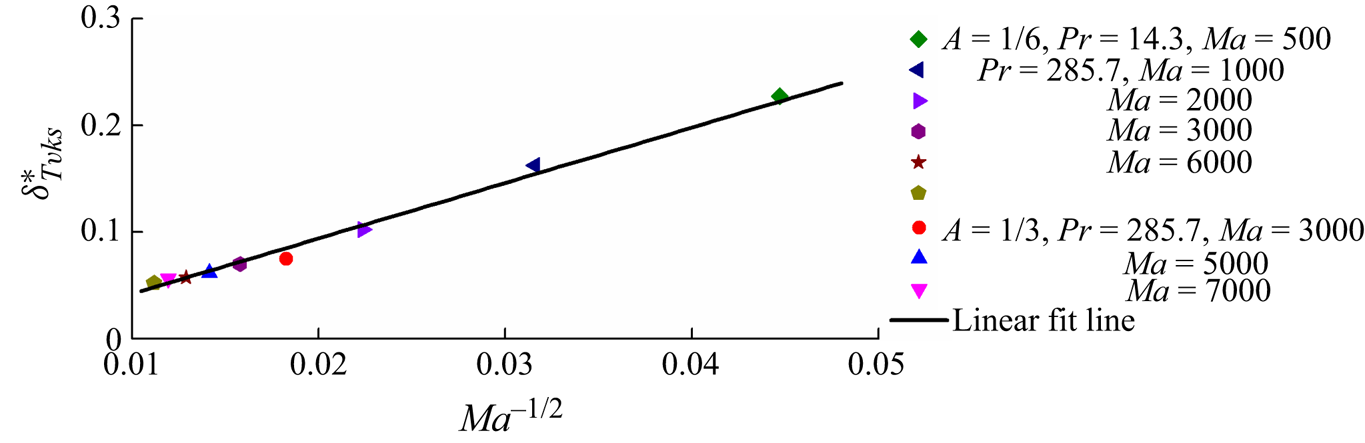
The scaling analysis indicates that after the sidewall is suddenly heated, heat transfer can occur, which results in a vertical thermal boundary layer specified by a scaling law (2.7). To validate (2.7), we measured a thickness of the vertical thermal boundary layer from numerical results. The thickness is defined as the distance from the sidewall to the isotherm of  ${T^\ast } = 0.05$ at
 ${y^\ast } = 0.5A$. Further, the thickness was normalized by (2.7) and is plotted in figure 8. It is clear that
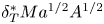 $\delta _T^\ast M{a^{1/2}}{A^{1/2}}$ is linear with
 ${({t^\ast }/t_{scs}^\ast )^{1/2}}$. This implies that (2.7) is verified by the numerical results. Further, the formula of the thickness may be obtained using a linear fit
 \begin{equation}\delta _T^\ast M{a^{1/2}}{A^{1/2}} = 2.6{({t^\ast }/t_{scs}^\ast )^{1/2}}.\end{equation}
Thickness in unsteady stage in ESs I.2 and I.3.
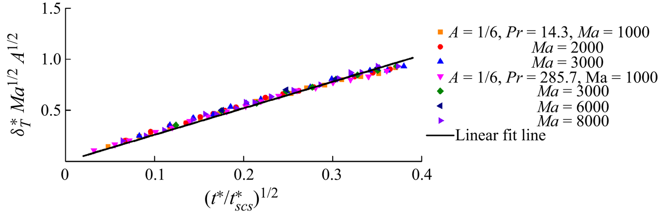
The thickness may increase with the passage of time in the unsteady stage, as shown in figure 8 and scaled by (2.7). Additionally, the scaling analysis also shows that the thickness may become a constant in the steady stage, as scaled by (2.54). For validation of (2.54), the distance between the sidewall and the isotherm of  ${T^\ast } = 0.7$ at
 ${y^\ast } = 0.25A$ in the steady stage was measured and is plotted in figure 9. Here, the isotherm of
 ${T^\ast } = 0.7$ at
 ${y^\ast } = 0.25A$ was selected to describe the thickness, which may reduce the disturbance from the circulation of the convective flow as shown in figure 7(f). Clearly, there is a linear function of
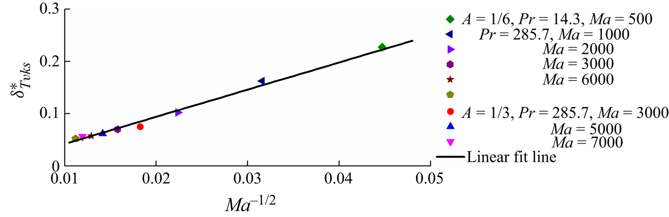
 $\delta _{T\nu \kappa s}^\ast $ and Ma −1/2, as shown in figure 9. That is, the scaling law is verified based on these numerical results. Further, adopting a linear fit, we may obtain
 \begin{equation}\delta _{T\nu \kappa s}^\ast= 5.2M{a^{ - 1/2}} - 0.01.\end{equation}
Thickness of vertical thermal boundary layer in the steady stage in ESs I.2 and I.3.
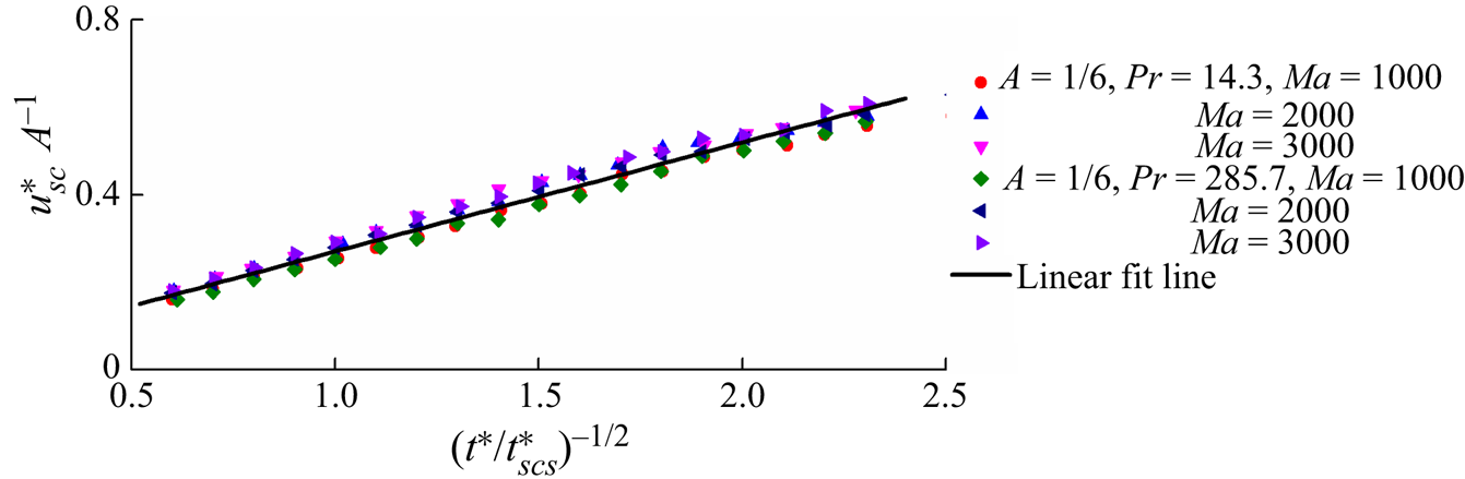
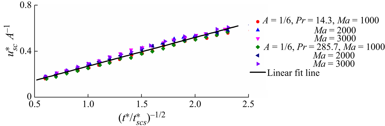
The scaling analysis in § 2 shows that a surface flow can be induced by a thermocapillary force generated by a non-uniform temperature distribution after sudden heating. The motion of the fluid in such a surface flow can be dominated by different regimes in different stages. Here, the velocity scale only in the VFDV stage was selected for validation because the early stages are too short. To verify the scaling law (2.18), the velocity for the isotherm of  ${T^\ast } = 0.05$ was extracted at
 ${y^\ast } = A$. The velocity normalized by (2.18) is shown in figure 10. It is clear that there is a linear function of
 $u_{sc}^\ast {A^{ - 1}}$ and
 ${({t^\ast }/t_{scs}^\ast )^{ - 1/2}}$; that is, (2.18) is coincident with the present numerical results. Further, we may obtain the formula based on linear fitting, given by
 \begin{equation}u_{sc}^\ast {A^{ - 1}} = 0.25{({t^\ast }/t_{scs}^\ast )^{ - 1/2}} + 0.02.\end{equation}
Velocity of surface flow in the VFDV stage in ESs I.2 and I.3.
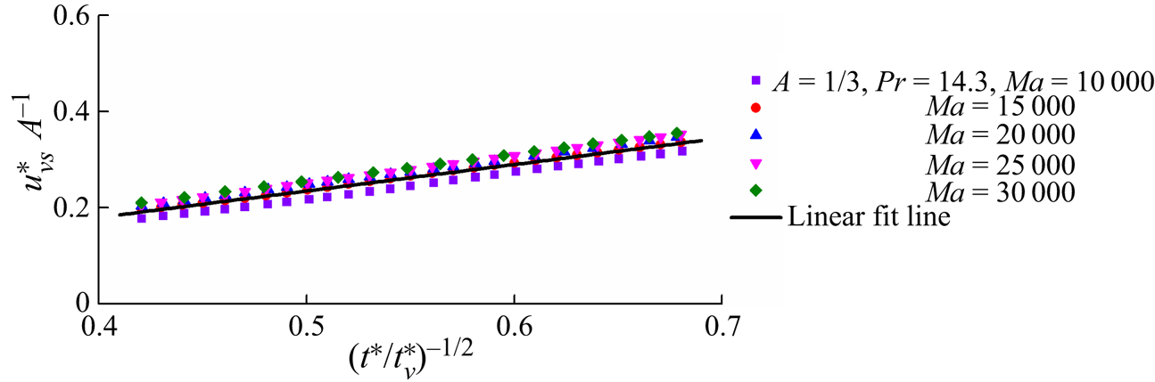
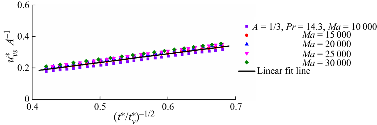
Further, to validate the velocity scale (2.21) of the surface flow in the FDVV stage in ES II, we measured the velocity for the isotherm of  ${T^\ast } = 0.05$, which is shown in figure 11. The numerical results describing the velocity in the FDVV stage are normalized using (2.21). A linear function of
 $u_{\nu s}^\ast {A^{ - 1}}$ and
 ${({t^\ast }/t_\nu ^\ast )^{1/2}}$ in figure 11 indicates that the scaling law (2.21) is coincident with the present numerical results. Further, we have obtained the formula for the velocity based on the linear fit,
 \begin{equation}u_{\nu s}^\ast {A^{ - 1}} = 0.55{({t^\ast }/t_\nu ^\ast )^{1/2}} - 0.04.\end{equation}
Velocity of surface flow in the FDVV stage in ES II.
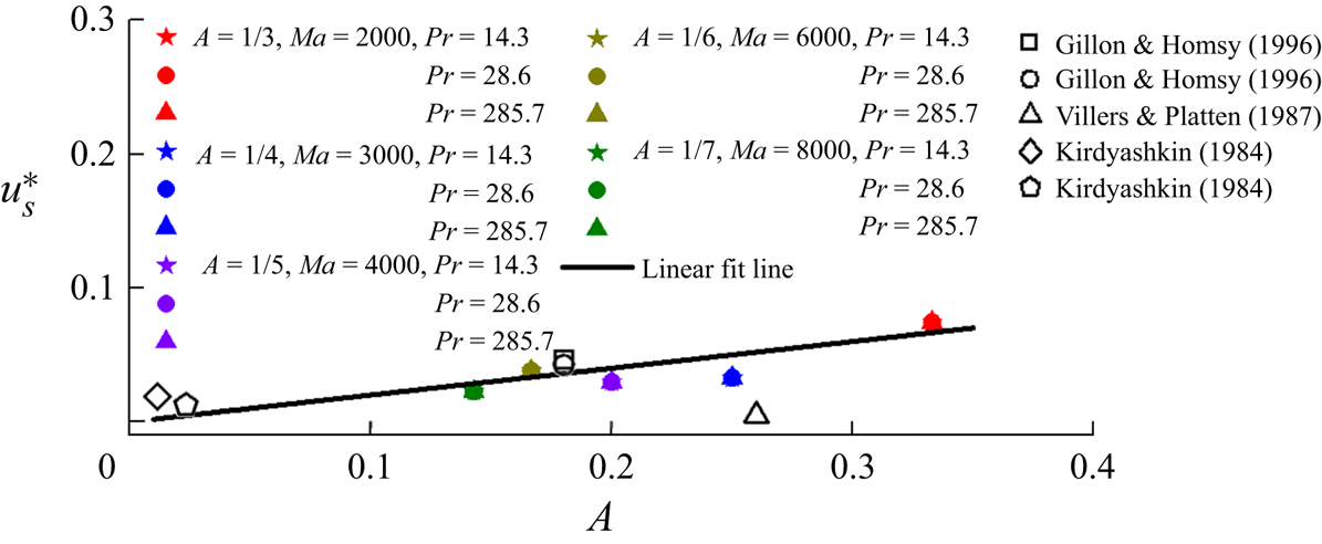
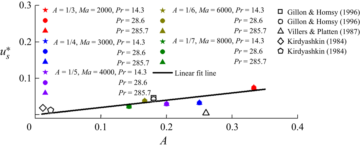
It is clear that the velocity becomes constant, as specified by (2.20). For validation of (2.20), we also calculated the velocity at  ${x^\ast } = 0.5$ and
 ${y^\ast } = A$ on the surface, which is shown in figure 12. An approximately linear relation between the velocity us and the aspect ratio A is clear. That is, (2.20) may scale the velocity in the FDVFDV stage in ESs I.1, I.2 and II. In this study, five aspect ratios were considered for reasonable cost. Additionally, the five velocities from the ground experiments are also shown in figure 12. Clearly, the scaling prediction is consistent with the experimental results but with visible differences. The differences may be attributed to the fact that the scaling and numerical results are two-dimensional and with zero gravity with the assumptions of a flat and non-volatile gas–liquid surface and an adiabatic upper boundary, but the ground experimental results are not (also see Kirdyashkin Reference Kirdyashkin1984; Villers & Platten Reference Villers and Platten1987; Gillon & Homsy Reference Gillon and Homsy1996). Further, the formula based on a linear fit is given by
 \begin{equation}u_s^\ast= 0.2A.\end{equation}
Velocity of surface flow in the FDVFDV stage in ESs I.1, I.2 and II. Here, all open symbols denote experimental results for which squares and circles are taken from figures 3 and 5 in Gillon & Homsy (Reference Gillon and Homsy1996), triangles are taken from figure 12 in Villers & Platten (Reference Villers and Platten1987) and diamonds and pentagons are taken from figures 4 and 9 in Kirdyashkin (Reference Kirdyashkin1984).
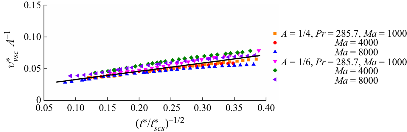
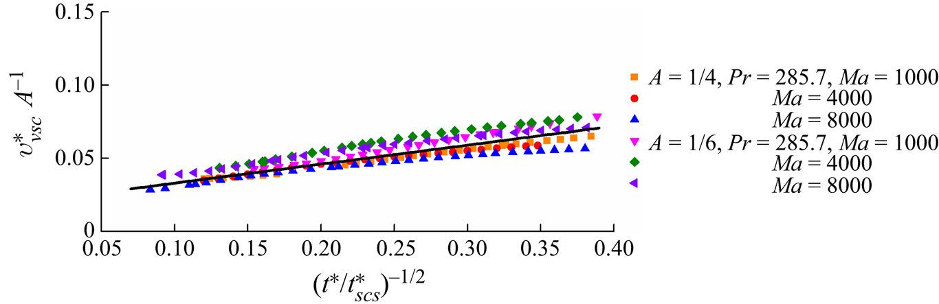
The surface flow driven by the thermocapillary force may further induce vertical flow adjacent to the heated sidewall. The discussion in § 2.2 shows that the vertical flow may also move under different regimes, as described by the scaling law (2.45). For validation, the velocity at  ${x^\ast } = 0.05$ and y* = 0.5A was calculated. The velocity extracted from the numerical results is plotted in figure 13, which is normalized by (2.45). Clearly, there is an approximately linear relation between
 $v_{\nu sc}^\ast {A^{ - 1}}$ and
 ${({t^\ast }/t_{scs}^\ast )^{ - 1/2}}$ with data scatter. This is because the circulation shown in figure 7(f) actually moves with the increase of the Marangoni number, disturbing the extraction of the velocity of the vertical flow, which cannot be considered in the scaling analysis. The formula for the velocity obtained by a linear fit is expressed as
 \begin{equation}v_{\nu sc}^\ast {A^{ - 1}} = 0.13{({t^\ast }/t_{scs}^\ast )^{ - 1/2}} + 0.02.\end{equation}
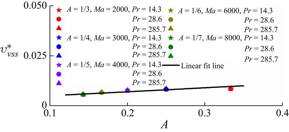
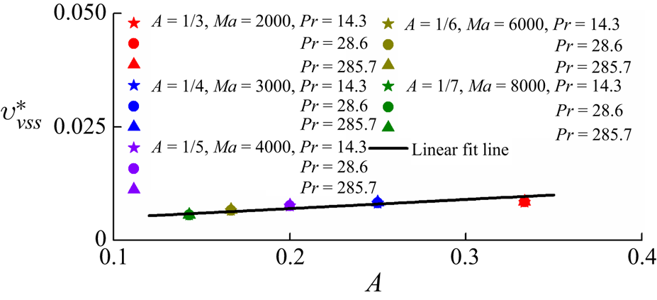
For further validation of the velocity of the vertical flow in the FDVFDV stage, the velocity at x* = 0.05 and y* = 0.5A was measured. The numerical results normalized by (2.52) are plotted in figure 14. An approximately linear relation between  $v_{\nu ss}^\ast $ and A is clear, suggesting that the scaling law (2.52) may be used to describe the vertical flow in the FDVFDV stage in ESs I.2, I.3 and II. Further, the formula based on the linear fit may be given by
 \begin{equation}v_{\nu ss}^\ast= 0.02A + 0.003.\end{equation}
Velocity of vertical flow in the VFDV stage in ESs. I.2 and I.3.
Velocity of vertical flow in the FDVFDV stage in ESs I.2 and I.3 and II.
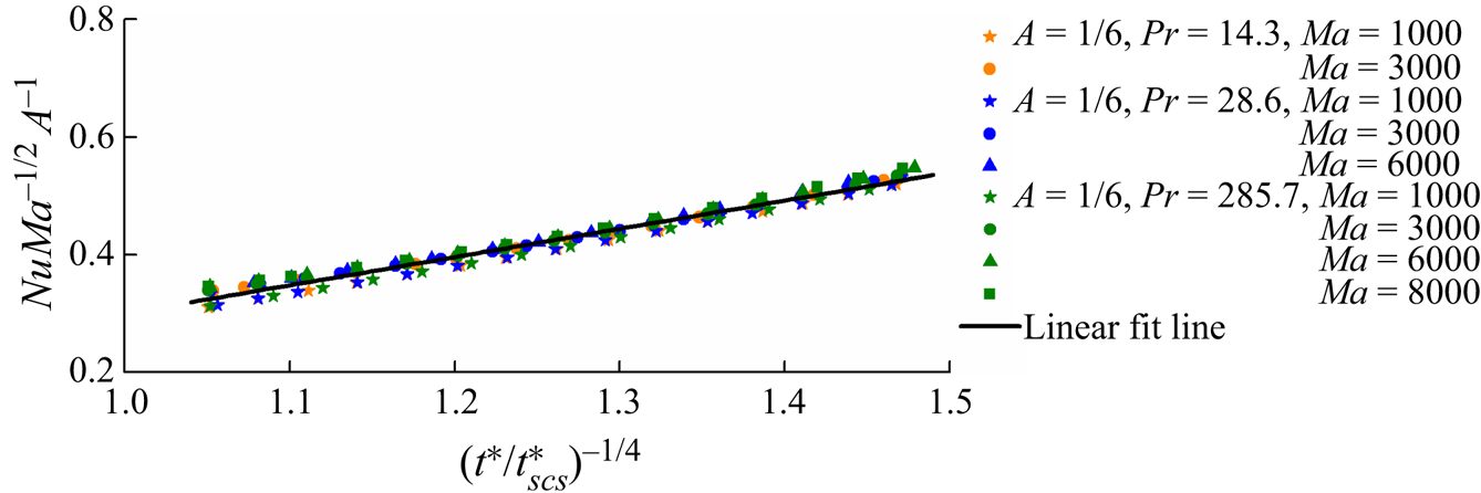
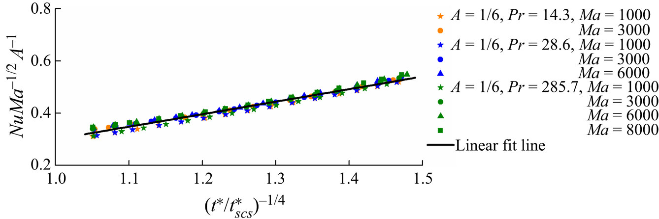
The scaling law (2.57) quantifies heat transfer adjacent to the heated sidewall. To validate (2.57), the Nusselt number of the heated sidewall was calculated from the numerical results and is plotted in figure 15. The good linear relation between NuMa −1/2A −1 and  ${({t^\ast }/t_{scs}^\ast )^{ - 1/4}}$ in figure 15 indicates that the scaling law (2.57) is able to quantify heat transfer in the VFDV stage in ESs I.2 and I.3. Additionally, the formula based on a linear fit may be expressed as
 \begin{equation}NuM{a^{ - 1/2}}{A^{ - 1}} = 0.48{({t^\ast }/t_{scs}^\ast )^{ - 1/4}} - 0.18.\end{equation}
Nusselt number for the heated sidewall in the VFDV stage in ESs I.2 and I.3.
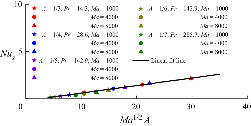
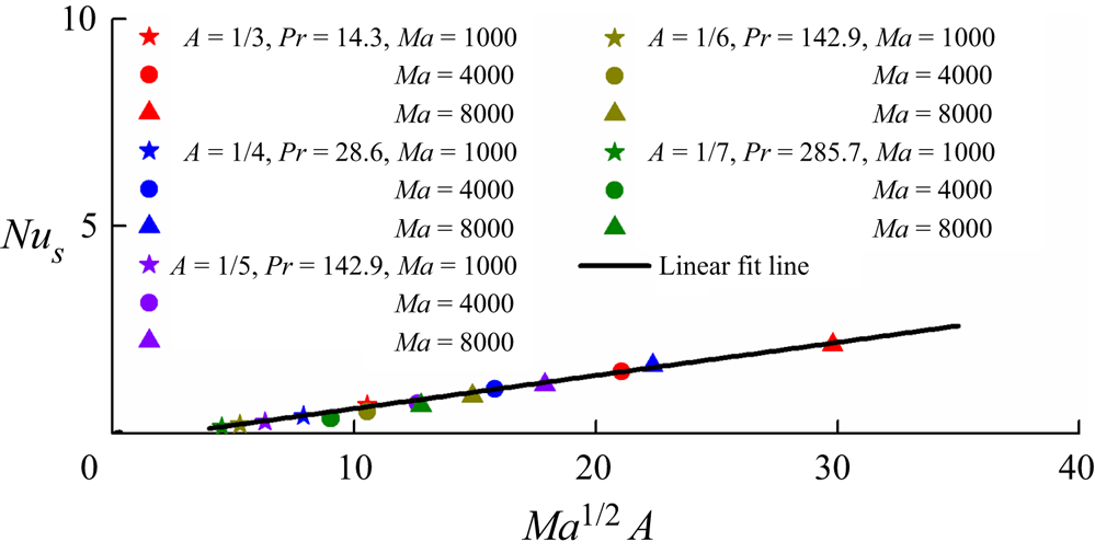
Furthermore, the Nusselt number of the heated sidewall in the steady stage Nus is also shown in figure 16. Clearly, Nus has a good linear relation with Ma 1/2A, which further verifies (2.57) in the FDVFDV stage. The formula in the steady stage based on a linear fit can be given by
 \begin{equation}N{u_s} = 0.08M{a^{1/2}}A - 0.2.\end{equation}
5. Conclusions
In this study, transient Marangoni convection in a rectangular pool for Pr > 1 and A < 1 is investigated using scaling analysis. A set of scaling laws describing transient Marangoni convection under different regimes in different ESs has been obtained.
Scaling analysis indicates that transient Marangoni convection after sudden heating can be classified to five regimes in different ESs. In particular, the dynamical evolution and the thermal process in ES I (the case of  $Ma < A_\varepsilon ^{ - 1}$ and A −1 < Ma < PrA −3) have been analysed under consideration of the most practical cases, and the dynamical evolution and the thermal process in ES II (the case of
 $Pr{A^{ - 3}} < Ma < A_\varepsilon ^{ - 1}$) have also been presented in Appendix A.
In ES I, transient Marangoni convection may be classified into three possible ESs. For A −1 < Ma < A −2 and  $Ma < A_\varepsilon ^{ - 1}$, there is no distinct vertical thermal boundary layer and heat transfer is under the conduction regime. For Ma > A −2, Ma < PrA −1 and
 $Ma < A_\varepsilon ^{ - 1}$, the convection flow is weak. The vertical flow is dominated by a viscous regime and heat transfer is under the conduction and convection regimes in sequence. For Ma > A −2, PrA −1 < Ma < PrA −3 and
 $Ma < A_\varepsilon ^{ - 1}$, the vertical flow may be dominated by viscous, inertial and again viscous regimes in sequence, and heat transfer may encounter the conduction and convection regimes in sequence.
Further, 2-D numerical simulation has been performed for different Ma, Pr and A to validate selected scaling laws. The scaling predictions are consistent with the present numerical results. The scaling laws can describe transient Marangoni convection in a rectangular pool.
Nusselt number of the heated sidewall in the FDVFDV stage in ESs I.1, I.2 and II.
Funding
The authors would like to thank the Fundamental Research Funds for the Central Universities (No. 2021RC261) and the National Natural Science Foundation of China (11972072) for the financial support.
Declaration of interests
The authors report no conflict of interest.
Appendix A
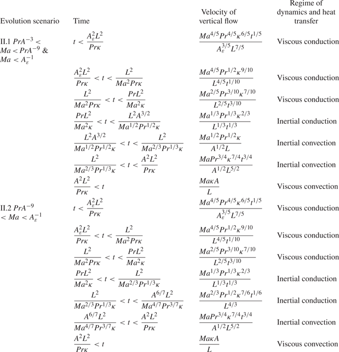
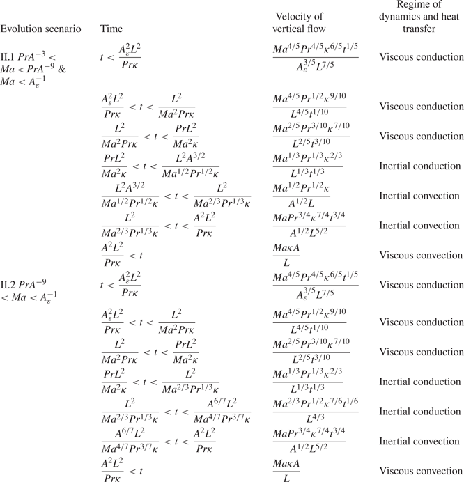
The ESs of the vertical flow induced by the surface flow in ES II (in the case of  $Pr{A^{ - 3}} < Ma < A_\varepsilon ^{ - 1}$) are analysed below. Since the vertical flow is driven by the surface flow induced pressure gradient adjacent to the sidewall, the dynamical evolution of the vertical flow will be discussed in the CI, CV, VV, FDVV and FDVFDV stages in sequence in the following section (also see table 1).
(a) CI stage
Regimes of dynamics and heat transfer of the vertical flow are the same as those in ES I in § 2.2.2 (a).
(b) CV stage
Regimes of dynamics and heat transfer of the vertical flow are also the same as those in ES I in § 2.2.2 (b).
(c) VV stage
In this stage, xT ~ ut. Additionally, the penetration distance of the vertical flow is vt for t < H/v and H for t ≥ H/v. That is, (2.22) may be expressed as
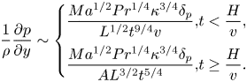 \begin{equation}\frac{1}{\rho }\frac{{\partial p}}{{\partial y}}\sim \left\{ {\begin{array}{*{20}{@{}l}} {\dfrac{{M{a^{1/2}}P{r^{1/4}}{\kappa^{3/4}}{\delta_p}}}{{{L^{1/2}}{t^{9/4}}v}},}&{t < \dfrac{H}{v},}\\ {\dfrac{{M{a^{1/2}}P{r^{1/4}}{\kappa^{3/4}}{\delta_p}}}{{A{L^{3/2}}{t^{5/4}}}},}&{t \ge \dfrac{H}{v}.} \end{array}} \right.\end{equation}
Further, the rate of the surface flow is equivalent to that in the vertical flow
 \begin{equation}{Q_{\nu c}}\sim {u_{\nu c}}{\varDelta _\nu }\sim \frac{{M{a^{1/2}}P{r^{3/4}}{\kappa ^{5/4}}{t^{1/4}}}}{{{L^{1/2}}}}.\end{equation}
Repeating the analysis of (2.26) and (2.27), based on (A1) and (A2), we may obtain the velocity and the thickness under a thermocapillary inertial regime
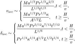 \begin{equation}\begin{array}{c} {v_{i\nu c}}\sim \left\{ {\begin{array}{*{20}{@{}l}} {\dfrac{{M{a^{1/3}}P{r^{1/3}}{\kappa^{2/3}}}}{{{L^{1/3}}{t^{1/3}}}},}&{t < \dfrac{H}{v},}\\ {\dfrac{{M{a^{1/2}}P{r^{1/2}}\kappa }}{{{A^{1/2}}L}},}&{t \ge \dfrac{H}{v},} \end{array}} \right.\\ {\delta _{i\nu c}}\sim \left\{ {\begin{array}{*{20}{@{}l}} {\dfrac{{M{a^{1/6}}P{r^{5/12}}{\kappa^{7/12}}{t^{7/12}}}}{{{L^{{1 / 6}}}}},}&{t < \dfrac{H}{v},}\\ {P{r^{1/4}}{\kappa^{1/4}}{A^{1/2}}{L^{1/2}}{t^{1/4}},}&{t \ge \dfrac{H}{v},} \end{array}} \right. \end{array}\end{equation}
and under a thermocapillary viscous regime
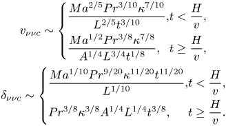 \begin{equation}\begin{array}{c} {v_{\nu \nu c}}\sim \left\{ {\begin{array}{*{20}{@{}l}} {\dfrac{{M{a^{2/5}}P{r^{3/10}}{\kappa^{7/10}}}}{{{L^{2/5}}{t^{3/10}}}},}&{t < \dfrac{H}{v},}\\ {\dfrac{{M{a^{1/2}}P{r^{3/8}}{\kappa^{7/8}}}}{{{A^{1/4}}{L^{3/4}}{t^{1/8}}}},}&{t \ge \dfrac{H}{v},} \end{array}} \right.\\ {\delta _{\nu \nu c}}\sim \left\{ {\begin{array}{*{20}{@{}l}} {\dfrac{{M{a^{1/10}}P{r^{9/20}}{\kappa^{11/20}}{t^{11/20}}}}{{{L^{1/10}}}},}&{t < \dfrac{H}{v},}\\ {P{r^{3/8}}{\kappa^{3/8}}{A^{1/4}}{L^{1/4}}{t^{3/8}},}&{t \ge \dfrac{H}{v}.} \end{array}} \right. \end{array}\end{equation}
Let the inertial term be equivalent to the viscous term, based on either (A1) or (A2), we further obtain a time scale
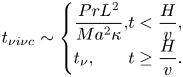 \begin{equation}{t_{\nu i\nu c}}\sim \left\{ {\begin{array}{*{20}{@{}l}} {\dfrac{{Pr{L^2}}}{{M{a^2}\kappa }},}&{t < \dfrac{H}{v},}\\ {{t_\nu },}&{t \ge \dfrac{H}{v}.} \end{array}} \right.\end{equation}
It is clear that tνiνc/tνκκ > 1 and  ${t_{\nu i\nu c}}/{t_{\nu cs}}\sim {(Pr/Ma)^{3/4}} < 1$ if the penetration distance vt < H or tνiνc/tνcs ~ (MaA 3/Pr)2/3 > 1 if the penetration distance vt ≥ H. This means that the vertical flow is firstly under a thermocapillary viscous regime in the VV stage.
Consider the vertical thermal boundary layer adjacent to the sidewall. In the energy equation (2.4), we have vt ~ H if the convection term O(vT/H) and the conduction term O(T/t) become equivalent. Using (A4), the time scale for the balance between the conduction term and the convection term may be expressed as
 \begin{equation}{t_{\nu \kappa \nu c}}\sim \frac{{{L^2}{A^{10/7}}}}{{M{a^{4/7}}P{r^{3/7}}\kappa }},\quad {t_{i\kappa \nu c}}\sim \frac{{{L^2}{A^{3/2}}}}{{M{a^{1/2}}{{\Pr }^{1/2}}\kappa }}.\end{equation}
In fact, tνκνc is the time scale at which the length scale of the vertical pressure gradient becomes H. Further, we may have  ${t_{\nu \kappa \nu c}}/{t_{\nu \kappa \kappa }}\sim {(MaPrA)^{10/7}} > 1$,
 ${t_{\nu \kappa \nu c}}/{t_{\nu cs}}\sim {(Ma{A^{15}}/Pr)^{2/21}}$,
 ${t_{\nu \kappa \nu c}}/{t_{\nu i\nu c}}\sim {(MaA/Pr)^{10/7}} > 1$ if the penetration distance vt < H or (Pr/MaA)4/7 < 1 if the penetration distance vt ≥ H,
 ${t_{i\kappa \nu c}}/{t_{\nu i\nu c}}\sim {(MaA/Pr)^{3/2}} > 1$ if the penetration distance vt < H and
 ${t_{i\kappa \nu c}}/{t_{\nu cs}}\sim {(Ma{A^9}/Pr)^{1/6}}$. That is, in the case of
 $Pr{A^{ - 3}} < Ma < Pr{A^{ - 9}}({t_{\nu i\nu c}} < {t_{i\kappa \nu c}} < {t_{\nu cs}})$, the vertical flow is dominated by a thermocapillary viscous regime under the balance between unsteady and conduction terms when tνκκ < t < tνiνc, by a thermocapillary inertial regime under the balance between unsteady and conduction terms when tνiνc < t < tiκνc and by a thermocapillary inertial regime under the balance between convection and conduction terms when tiκνc < t < tνcs. According to (A3), the convection term balances the conduction term in (2.4), which yields the thickness when tiκνc < t < tνcs in the case of PrA −3 < Ma < PrA −9
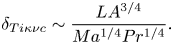 \begin{equation}{\delta _{Ti\kappa \nu c}}\sim \frac{{L{A^{3/4}}}}{{M{a^{1/4}}P{r^{1/4}}}}.\end{equation}
In the case of  $Ma > Pr{A^{ - 9}}({t_{\nu i\nu c}} < {t_{\nu cs}} < {t_{i\kappa \nu c}})$, the vertical flow is dominated by a thermocapillary viscous regime under the balance between unsteady and conduction terms when tνκκ < t < tνiνc, and by a thermocapillary inertial regime under the balance between unsteady and conduction terms when tνiνc < t < tνcs.
(d) FDVV stage
In this stage, xT ~ L. The analysis shows that the penetration distance of the vertical flow is H in the case of PrA −3 < Ma < PrA −9 but vt for t < H/v and H for t ≥ H/v in the case of Ma > PrA −9. Thus, (2.22) is expressed as
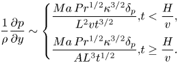 \begin{equation}\frac{1}{\rho }\frac{{\partial p}}{{\partial y}}\sim \left\{ {\begin{array}{*{20}{@{}l}} {\dfrac{{Ma\,P{r^{1/2}}{\kappa^{3/2}}{\delta_p}}}{{{L^2}v{t^{{3 / 2}}}}},}&{t < \dfrac{H}{v},}\\ {\dfrac{{Ma\,P{r^{1/2}}{\kappa^{3/2}}{\delta_p}}}{{A{L^3}{t^{1/2}}}},}&{t \ge \dfrac{H}{v}.} \end{array}} \right.\end{equation}
Further, the rate of the vertical flow supplying the surface flow may be given by
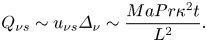 \begin{equation}{Q_{\nu s}}\sim {u_{\nu s}}{\varDelta _\nu }\sim \frac{{MaPr{\kappa ^2}t}}{{{L^2}}}.\end{equation}
Repeating the analysis of (2.26) and (2.27), based on (A8) and (A9), we may obtain the velocity and the thickness under a thermocapillary inertial regime
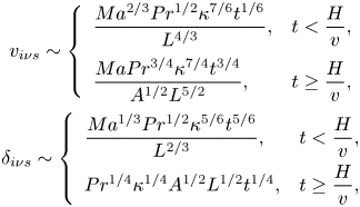 \begin{equation}\begin{array}{@{}c} {v_{i\nu s}}\sim \left\{ {\begin{array}{*{20}{l}} {\dfrac{{M{a^{2/3}}P{r^{1/2}}{\kappa^{7/6}}{t^{1/6}}}}{{{L^{4/3}}}},}&{t < \dfrac{H}{v},}\\ {\dfrac{{MaP{r^{3/4}}{\kappa^{7/4}}{t^{3/4}}}}{{{A^{1/2}}{L^{5/2}}}},}&{t \ge \dfrac{H}{v},} \end{array}} \right.\\ {\delta _{i\nu s}}\sim \left\{ {\begin{array}{*{20}{l}} {\dfrac{{M{a^{1/3}}P{r^{1/2}}{\kappa^{5/6}}{t^{5/6}}}}{{{L^{{2 / 3}}}}},}&{t < \dfrac{H}{v},}\\ {P{r^{1/4}}{\kappa^{1/4}}{A^{1/2}}{L^{1/2}}{t^{1/4}},}&{t \ge \dfrac{H}{v},} \end{array}} \right. \end{array}\end{equation}
and under a thermocapillary viscous regime
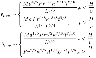 \begin{equation}\begin{array}{@{}c} {v_{\nu \nu s}}\sim \left\{ {\begin{array}{*{20}{@{}l}} {\dfrac{{M{a^{{4 / 5}}}P{r^{1/2}}{\kappa^{13/10}}{t^{3/10}}}}{{{L^{8/5}}}},}&{t < \dfrac{H}{v},}\\ {\dfrac{{Ma\,P{r^{5/8}}{\kappa^{13/8}}{t^{5/8}}}}{{{A^{1/4}}{L^{9/4}}}},}&{t \ge \dfrac{H}{v},} \end{array}} \right.\\ {\delta _{\nu \nu s}}\sim \left\{ {\begin{array}{*{20}{@{}l}} {\dfrac{{M{a^{1/5}}P{r^{1/2}}{\kappa^{7/10}}{t^{7/10}}}}{{{L^{2/5}}}},}&{t < \dfrac{H}{v},}\\ {P{r^{3/8}}{\kappa^{3/8}}{A^{1/4}}{L^{1/4}}{t^{3/8}},}&{t \ge \dfrac{H}{v}.} \end{array}} \right. \end{array}\end{equation}
Similar to the discussion of (2.33), letting the inertial term be equivalent to the viscous term, based on equation either (A10) or (A11), we obtain a time scale
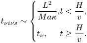 \begin{equation}{t_{\nu i\nu s}}\sim \left\{ {\begin{array}{*{20}{@{}l}} {\dfrac{{{L^2}}}{{Ma\kappa }},}&{t < \dfrac{H}{v},}\\ {{t_\nu },}&{t \ge \dfrac{H}{v}.} \end{array}} \right.\end{equation}
The further analysis shows that tνiνs < tνcs for Ma > PrA −9 and tνiνs ~ tν for PrA −3 < Ma < PrA −9. This means that a vertical flow can be dominated by a thermocapillary inertial regime in the FDVV stage.
Consider the vertical thermal boundary layer adjacent to the sidewall. In the energy equation (2.4), the unsteady term is O(T/t), and the convection term is O(vT/H). A time scale for the balance between unsteady term and convection term may be expressed as
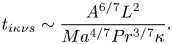 \begin{equation}{t_{i\kappa \nu s}}\sim \frac{{{A^{6/7}}{L^2}}}{{M{a^{4/7}}P{r^{3/7}}\kappa }}.\end{equation}
Based on (2.9), in the case of  $Pr{A^{ - 3}} < Ma < Pr{A^{ - 9}}({t_{i\kappa \nu s}} < {t_{\nu cs}})$, heat transfer of the vertical thermal boundary layer is under the balance between convection and conduction terms in the FDVV stage. In the case of
 $Ma > Pr{A^{ - 9}}({t_{\nu cs}} < {t_{i\kappa \nu s}} < {t_\nu })$, heat transfer of the vertical thermal boundary layer is under the balance between unsteady and conduction terms when tνcs < t < tiκνs and under the balance between convection and conduction terms when tiκνs < t < tν. The balance between convection and conduction terms yields the thickness of the vertical thermal boundary layer in the case of PrA −3 < Ma < PrA −9 and when tiκνs < t < tν in the case of Ma > PrA −9
 \begin{equation}{\delta _{Ti\kappa \nu s}}\sim \frac{{{A^{3/4}}{L^{7/4}}}}{{M{a^{1/2}}P{r^{3/8}}{\kappa ^{3/8}}{t^{3/8}}}}.\end{equation}
(e) FDVFDV stage
In this stage, Δν ~ H and xT ~ L. According to the analysis in the FDVV stage, the penetration distance of the vertical flow is H. Equation (2.22) may be expressed as
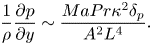 \begin{equation}\frac{1}{\rho }\frac{{\partial p}}{{\partial y}}\sim \frac{{MaPr{\kappa ^2}{\delta _p}}}{{{A^2}{L^4}}}.\end{equation}
The rate of a vertical flow supplying a surface flow is
 \begin{equation}{Q_{ss}}\sim {u_s}{\varDelta _\nu }\sim Ma\kappa {A^2}.\end{equation}
Repeating the analysis of (2.26) and (2.27), based on (A15) and (A16), we may obtain the velocity and the thickness under a thermocapillary inertial regime
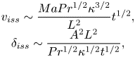 \begin{equation}\begin{array}{c} {v_{iss}}\sim \dfrac{{MaP{r^{1/2}}{\kappa ^{3/2}}}}{{{L^2}}}{t^{1/2}},\\ {\delta _{iss}}\sim \dfrac{{{A^2}{L^2}}}{{P{r^{1/2}}{\kappa ^{1/2}}{t^{1/2}}}}, \end{array}\end{equation}
and under a thermocapillary viscous regime
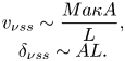 \begin{equation}\begin{array}{c} {v_{\nu ss}}\sim \dfrac{{Ma\kappa A}}{L},\\ {\delta _{\nu ss}}\sim AL. \end{array}\end{equation}
Similar to the discussion of (2.33), letting the inertial term be equivalent to the viscous term based on equation either (A15) or (A16), we have a time scale tνiss ~ tν. When t > tνiss, the inertial term is small. Therefore, the vertical flow is dominated by a thermocapillary viscous regime in the FDVFDV stage.
Consider the vertical thermal boundary layer adjacent to the sidewall. In the energy equation (2.4), the unsteady conduction term is O(T/t), and the convection term is O(vT/H). The balance between the two terms shows that the vertical thermal boundary layer becomes steady. The time scale to reach the steady state is
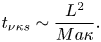 \begin{equation}{t_{\nu \kappa s}}\sim \frac{{{L^2}}}{{Ma\kappa }}.\end{equation}
It is clear that tνκs/tν < 1. This means that the thickness of the vertical thermal boundary layer becomes a constant value in the FDVFDV stage. The balance between the convection term and the conduction term in (2.4) yields the thickness of the vertical thermal boundary layer in the FDVFDV stage
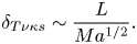 \begin{equation}{\delta _{T\nu \kappa s}}\sim \frac{L}{{M{a^{1/2}}}}.\end{equation}
The heat flux through the sidewall may be described by O(λΔT/δT) and normalized by λΔT/H. Thus, we may obtain the Nusselt number (Nu) for PrA −3 < Ma < PrA −9 based on (2.7), (A7), (A14) and (A20)
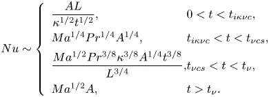 \begin{equation}Nu\sim \left\{ {\begin{array}{*{20}{l@{}}} {\dfrac{{AL}}{{{\kappa^{1/2}}{t^{1/2}}}},}&{0 < t < {t_{i\kappa \nu c}},}\\ {M{a^{1/4}}P{r^{1/4}}{A^{1/4}},}&{{t_{i\kappa \nu c}} < t < {t_{\nu cs}},}\\ {\dfrac{{M{a^{1/2}}P{r^{3/8}}{\kappa^{3/8}}{A^{1/4}}{t^{3/8}}}}{{{L^{3/4}}}},}&{{t_{\nu cs}} < t < {t_\nu },}\\ {M{a^{1/2}}A,}&{t > {t_\nu }.} \end{array}} \right.\end{equation}
and for Ma > PrA −9 based on (2.7), (A14) and (A20)
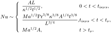 \begin{equation}Nu\sim \left\{ {\begin{array}{*{20}{l@{}}} {\dfrac{{AL}}{{{\kappa^{1/2}}{t^{1/2}}}},}&{0 < t < {t_{i\kappa \nu s}},}\\ {\dfrac{{M{a^{1/2}}{{\Pr }^{3/8}}{\kappa^{3/8}}{A^{1/4}}{t^{3/8}}}}{{{L^{3/4}}}},}&{{t_{i\kappa \nu s}} < t < {t_\nu },}\\ {M{a^{1/2}}A,}&{t > {t_\nu }.} \end{array}} \right.\end{equation}
The above-mentioned evolutions and regimes of dynamics and heat transfer of the vertical flow are listed in table 4.
Vertical flow under different regimes in ES II. Here, viscous denotes that the vertical flow is under the balance between the thermocapillary induced pressure gradient term and the viscous term, and inertial denotes that the vertical flow is under the balance between the thermocapillary induced pressure gradient term and the inertial term.