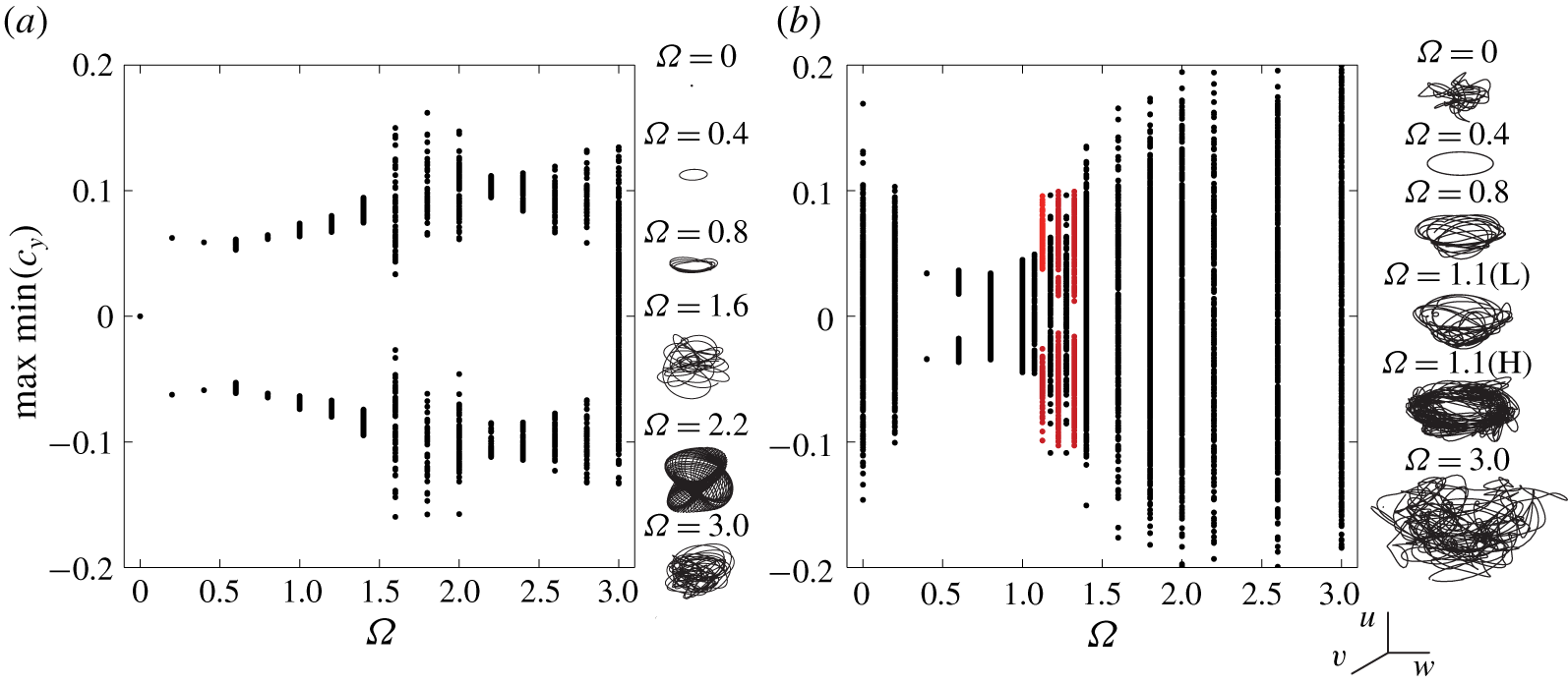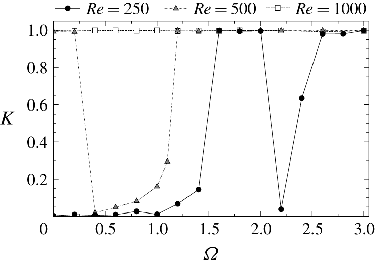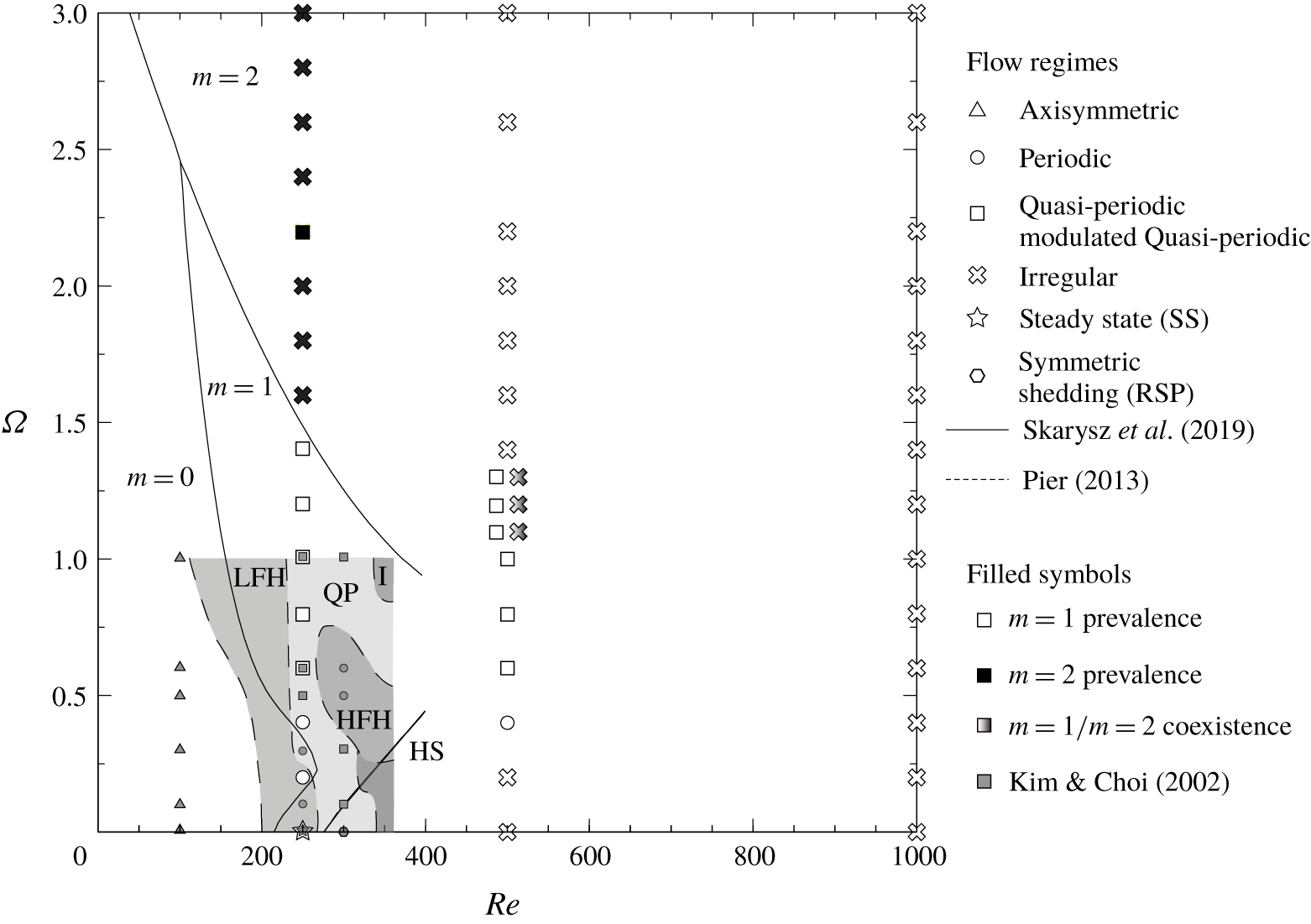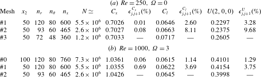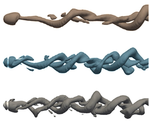


1 Introduction
The flow past rotating spheres can be found in many natural phenomena and engineering applications, for instance, in the transport of droplets and particles (Clift, Grace & Weber Reference Clift, Grace and Weber1978; Liu & Bogy Reference Liu and Bogy2008; Dgheim et al. Reference Dgheim, Abdallah, Habchi and Zakhia2012) or the design of micro-robots (Peyer et al. Reference Peyer, Mahoney, Zhang, Abbott and Nelson2012), whose motion depends on the forces distributions acting on their surface and, consequently, on the flow regimes, which are highly dependent of the direction of body rotation. Most of the work devoted to investigate the flow around rotating bodies is related to configurations with the axis of rotation placed perpendicularly to the free stream direction (transverse rotation) or aligned with it (streamwise rotation). Recent numerical and experimental studies have focused on the flow topology and stability modifications experimented in the wake as the rotation speed increases, which lead to important drag and lift coefficients variations, such as that described by the Magnus effect (Barkla & Auchterlone Reference Barkla and Auchterlone1971). In that sense, either transverse or streamwise rotation are shown to modify the pattern of bifurcations described for a fixed sphere (see, e.g. Sakamoto & Haniu Reference Sakamoto and Haniu1990; Johnson & Patel Reference Johnson and Patel1999; Fabre, Auguste & Magnaudet Reference Fabre, Auguste and Magnaudet2008) at low Reynolds numbers,  $Re$. In particular, the wake instability threshold for a static sphere is well established around
 $Re_{c1}\simeq 212$, which leads to a steady symmetric bifid wake (SS mode, Fabre et al. Reference Fabre, Auguste and Magnaudet2008), followed by a Hopf bifurcation at
 $Re_{c2}\simeq 272$, representing the onset of vortex shedding, which is set while keeping the axial reflectional symmetry plane (Fabre et al. Reference Fabre, Auguste and Magnaudet2008). This planar symmetry in the shedding process is lost around
 $Re_{c3}\simeq 375$, from which the wake starts to oscillate transversely (Chrust, Goujon-Durand & Wesfreid Reference Chrust, Goujon-Durand and Wesfreid2013).
Most recent works have widely dealt with modifications induced by transverse rotation for moderate values of the rotation parameter  $\unicode[STIX]{x1D6FA}=\unicode[STIX]{x1D714}D/2u_{\infty }$, where
 $\unicode[STIX]{x1D714}$,
 $D$ and
 $u_{\infty }$ are respectively the sphere’s angular velocity, its diameter and the free stream velocity. Generally, these analyses have been limited to the parametric region
 $Re\leqslant 350$ and
 $\unicode[STIX]{x1D6FA}\leqslant 1$ (Kurose & Komori Reference Kurose and Komori1999; Kim & Choi Reference Kim and Choi2002; Niazmand & Renksizbulut Reference Niazmand and Renksizbulut2003; Giacobello, Ooi & Balachandar Reference Giacobello, Ooi and Balachandar2009), wherein transverse rotation leads to unsteadiness in the wake at lower values of
 $Re$ than for a fixed sphere, while increasing the drag and promoting new instability regimes that foster lift. Recently, such flow has been analysed in terms of global instability (Citro et al. Reference Citro, Tchoufag, Fabre, Giannetti and Luchini2016), unveiling that the steady pitchfork bifurcation at
 $Re_{c1}$ is changed into an imperfect bifurcation, while at low values of
 $Re$ and
 $\unicode[STIX]{x1D6FA}>0.7$ a second unstable unsteady shedding mode appears.
The modification of the axis of rotation results in a completely different wake instability picture, as Poon et al. (Reference Poon, Ooi, Giacobello and Cohen2010) demonstrated numerically by varying the inclination of the rotation axis. In the limit, streamwise rotation already sets the wake unsteadiness at  $Re_{c1}$, and the steady state (SS) regime is substituted by a frozen rotation (Kim & Choi Reference Kim and Choi2002; Neeraj & Tiwari Reference Neeraj and Tiwari2018) of the bifid wake, in the sense that no change in the shape of the vortices exists while they spin around the axis. At higher values of
 $\unicode[STIX]{x1D6FA}$, these vortical structures adopt an helicoidal topology and rotate at a faster frequency. These two regimes have been related (Pier Reference Pier2013) to the destabilization of both low-frequency helical and high-frequency helical modes at
 $\unicode[STIX]{x1D6FA}\leqslant 1$ and
 $Re\leqslant 350$. In fact, frozen regimes are only circumscribed to some regions of the parametric map
 $Re-\unicode[STIX]{x1D6FA}$, and transitions between them are characterized by quasi-periodic or chaotic flow regimes. Moreover, they have been observed in wakes behind other axisymmetric geometries (Jiménez-González et al. Reference Jiménez-González, Sanmiguel-Rojas, Sevilla and Martínez-Bazán2013, Reference Jiménez-González, Sevilla, Sanmiguel-Rojas and Martínez-Bazán2014), proving that they stem from rotation-induced modifications of the aforementioned SS and reflectional symmetry preserving (RSP) modes.
In general, the flow past streamwise rotating spheres has received considerably less attention than transversely rotating spheres, and little is known on the effect of rotation in the wake behind the sphere for transitional regimes at Reynolds numbers larger than  $300$ and high values of the rotation parameter,
 $\unicode[STIX]{x1D6FA}>1$. In fact, wake regimes behind a streamwise rotating sphere seem to be comparatively more complex, already at
 $Re=350$, as Pier (Reference Pier2013) showed, denoting such regimes as irregular, since they show little coherence in the shedding process, especially at very low (
 $\unicode[STIX]{x1D6FA}<0.2$) and high (
 $0.8<\unicode[STIX]{x1D6FA}<1$) rotation rates. These regimes have been also characterized experimentally for
 $Re<400$ by Skarysz et al. (Reference Skarysz, Rokicki, Goujon-Durand and Wesfreid2018), using flow visualizations and modal decomposition techniques.
In any case, the origin of such complex transitions and subsequent regimes established in the wake behind streamwise rotating spheres, and their effect on the forces distributions, beyond these limits in the  $Re-\unicode[STIX]{x1D6FA}$ map, still remains unclear. Therefore, this paper aims to shed some light on this problem, by numerically investigating the effect of the streamwise rotation on the main characteristics of the flow around a sphere for transitional Reynolds numbers and high rotation velocities, i.e.
 $\unicode[STIX]{x1D6FA}\leqslant 3$. Within this region, we study the different unsteady flow regimes and instability mechanisms, related to helical global modes, along with variations on the forces coefficients distributions. The paper is structured as follows. The problem and numerical techniques employed, along with the validation studies for numerical schemes and mesh convergence are presented in § 2. Flow regimes for
 $Re=250,~500$ and 1000 are respectively introduced in §§ 3–5. The evolution of time-averaged force coefficients are presented in § 6, while bifurcation diagrams are studied in § 7. Finally, the main conclusions are outlined in § 8.
2 Problem description
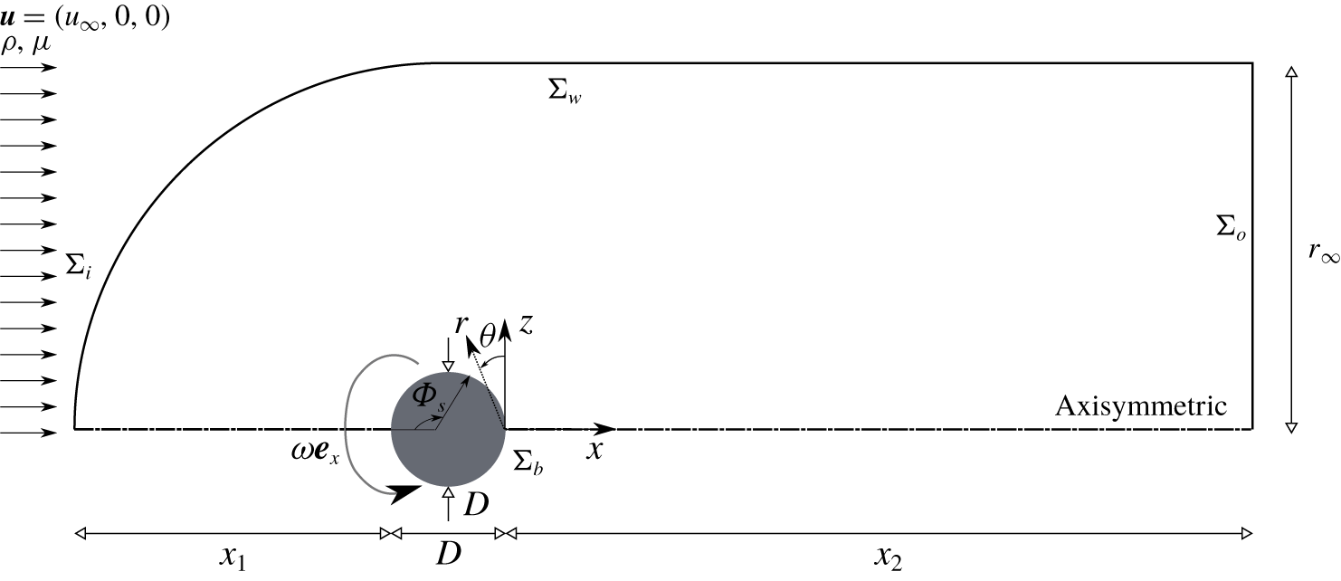
This study analyses the three-dimensional flow around a streamwise rotating sphere, as sketched in figure 1. A sphere of diameter  $D$ rotates with a constant angular velocity
 $\unicode[STIX]{x1D714}$ and is subjected to a free stream of velocity
 $u_{\infty }$, density
 $\unicode[STIX]{x1D70C}$ and viscosity
 $\unicode[STIX]{x1D707}$. The problem is then governed by two non-dimensional parameters, namely the Reynolds number
 $Re=\unicode[STIX]{x1D70C}u_{\infty }D/\unicode[STIX]{x1D707}=[250,500,1000]$ and the rotation parameter
 $\unicode[STIX]{x1D6FA}=\unicode[STIX]{x1D714}D/2u_{\infty }\leqslant 3$. The flow is described by the incompressible Navier–Stokes equations
 $$\begin{eqnarray}\displaystyle & \displaystyle \unicode[STIX]{x1D735}\boldsymbol{\cdot }\boldsymbol{u}=0, & \displaystyle\end{eqnarray}$$
 $$\begin{eqnarray}\displaystyle & \displaystyle \frac{\unicode[STIX]{x2202}\boldsymbol{u}}{\unicode[STIX]{x2202}t}+\boldsymbol{u}\boldsymbol{\cdot }\unicode[STIX]{x1D735}\boldsymbol{u}+\unicode[STIX]{x1D735}p-\frac{1}{Re}\unicode[STIX]{x1D6FB}^{2}\boldsymbol{u}=0, & \displaystyle\end{eqnarray}$$
where  $\boldsymbol{u}=(u,v,w)$ is the velocity vector referred to a cylindrical
 $(x,r,\unicode[STIX]{x1D703})$ coordinates system whose origin can be placed at the rear point of the sphere, and
 $p$ is the pressure. Equations (2.1)–(2.2) are made non-dimensional using
 $D$,
 $u_{\infty }$,
 $D/u_{\infty }$ and
 $\unicode[STIX]{x1D70C}u_{\infty }^{2}$ as the characteristic length, velocity, time and pressure scales, respectively. In the following, all variables will be made dimensionless using these scales. For instance, the pressure coefficient
 $c_{p}$ will be defined as
 $$\begin{eqnarray}c_{p}=\frac{p-p_{\infty }}{0.5\unicode[STIX]{x1D70C}u_{\infty }^{2}},\end{eqnarray}$$
with  $p_{\infty }$ being the reference pressure.
Sketch of the flow configuration and variables used for numerical simulations.

As shown in figure 1(b), the net forces acting on the sphere can be decomposed into components along the Cartesian coordinates, i.e.  $\text{f}_{x}$,
 $\text{f}_{y}$ and
 $\text{f}_{z}$, which are made non-dimensional as
 $$\begin{eqnarray}c_{i}=\frac{\text{f}_{i}}{0.5\unicode[STIX]{x1D70C}u_{\infty }^{2}S},\end{eqnarray}$$
where  $c_{i}$ represents the time dependent force coefficient on
 $i=x,~y$ and
 $z$, and
 $S=\unicode[STIX]{x03C0}D^{2}/4$ is the sphere’s projected area. Thus,
 $c_{x}$ is the drag force coefficient, while
 $c_{y}$ and
 $c_{z}$ respectively correspond to the transverse force coefficients along the
 $y$-axis and
 $z$-axis in such a way that the total lift force coefficient is obtained by means of
 $$\begin{eqnarray}c_{l}=\sqrt{c_{y}^{2}+c_{z}^{2}}.\end{eqnarray}$$
On the other hand, frequencies of time histories,  $\unicode[STIX]{x1D710}$, are presented in non-dimensional form as
 $$\begin{eqnarray}f=\frac{\unicode[STIX]{x1D710}D}{u_{\infty }},\end{eqnarray}$$
where dominant frequencies will be calculated from the Fourier transform of the corresponding time evolutions. Finally, any time dependent variable will be denoted using lower case letters,  $a$, while its temporal averaging will be expressed by means of capital letters,
 $A=\overline{a}$. Thus, employing the Reynolds notation,
 $a(t)=A+a^{\prime }(t)$, with
 $A^{\prime }=\sqrt{\overline{a^{\prime 2}}}$ being the standard fluctuation.
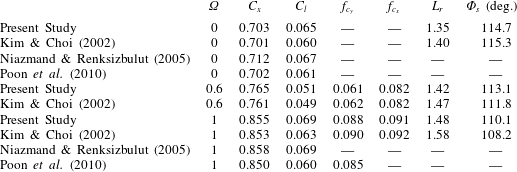
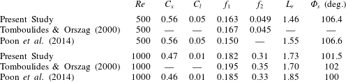
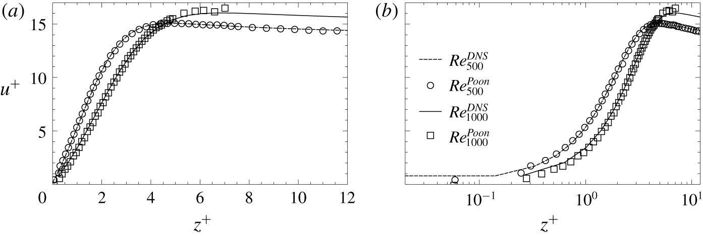
The flow governed by (2.1)–(2.2) is numerically solved using the finite-volumes toolbox OpenFOAM®, within the domain shown in figure 1, which consists of an upstream hemisphere of radius 15 and a downstream tube extending 50 diameters downstream of the body. Regarding the boundary conditions, a uniform streamwise velocity has been imposed at the inlet,  $\unicode[STIX]{x1D6F4}_{i}$,
 $\boldsymbol{u}=(1,0,0)$, while a no-slip boundary condition is fixed at the body surface,
 $\unicode[STIX]{x1D6F4}_{b}$, that rotates with constant angular velocity
 $\unicode[STIX]{x1D714}$, i.e.
 $\boldsymbol{u}=(0,0,\unicode[STIX]{x1D714}\cdot r)$. At the outlet,
 $\unicode[STIX]{x1D6F4}_{o}$, we impose an outflow condition that implements a Neumann condition for the velocity,
 $\boldsymbol{n}\boldsymbol{\cdot }\unicode[STIX]{x1D735}\boldsymbol{u}=0$, where
 $\boldsymbol{n}$ is the outward normal, and a Dirichlet condition for the pressure,
 $p=0$. The latter may be considered equivalent to setting a stress-free condition at the outlet for small values of the viscosity (as highlighted by Tomboulides & Orszag Reference Tomboulides and Orszag2000).
Finally, at the outer radial boundary,  $\unicode[STIX]{x1D6F4}_{w}$, we set a slip boundary condition,
 $\boldsymbol{n}\boldsymbol{\cdot }\boldsymbol{u}=0$. Note that the domain size and boundary conditions have been selected according to previous numerical works on rotating slender bodies and non-rotating spheres (see e.g. Jiménez-González Reference Jiménez-González2013). The reader is referred to appendix B for detailed information regarding the employed numerical schemes, and convergence and validation studies.
3 Flow regimes behind a streamwise rotating sphere at Re  $=$ 250

We will present in the following sections the results from numerical simulations, where the wake regimes and their dynamics are analysed in depth with the help of the modal decomposition techniques detailed in appendix B. To properly capture different flow regimes, and as a compromise between resolution and computational cost, simulations are performed with increments of  $\unicode[STIX]{x0394}\unicode[STIX]{x1D6FA}=0.2$ or 0.1 in those regions where transitions between regimes are more complex, in line with similar studies existing in the literature.
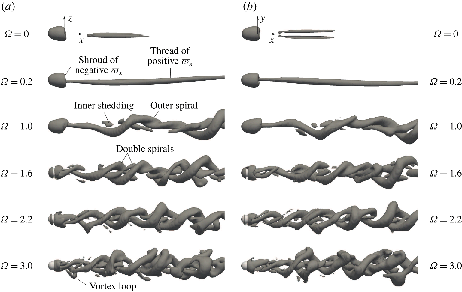
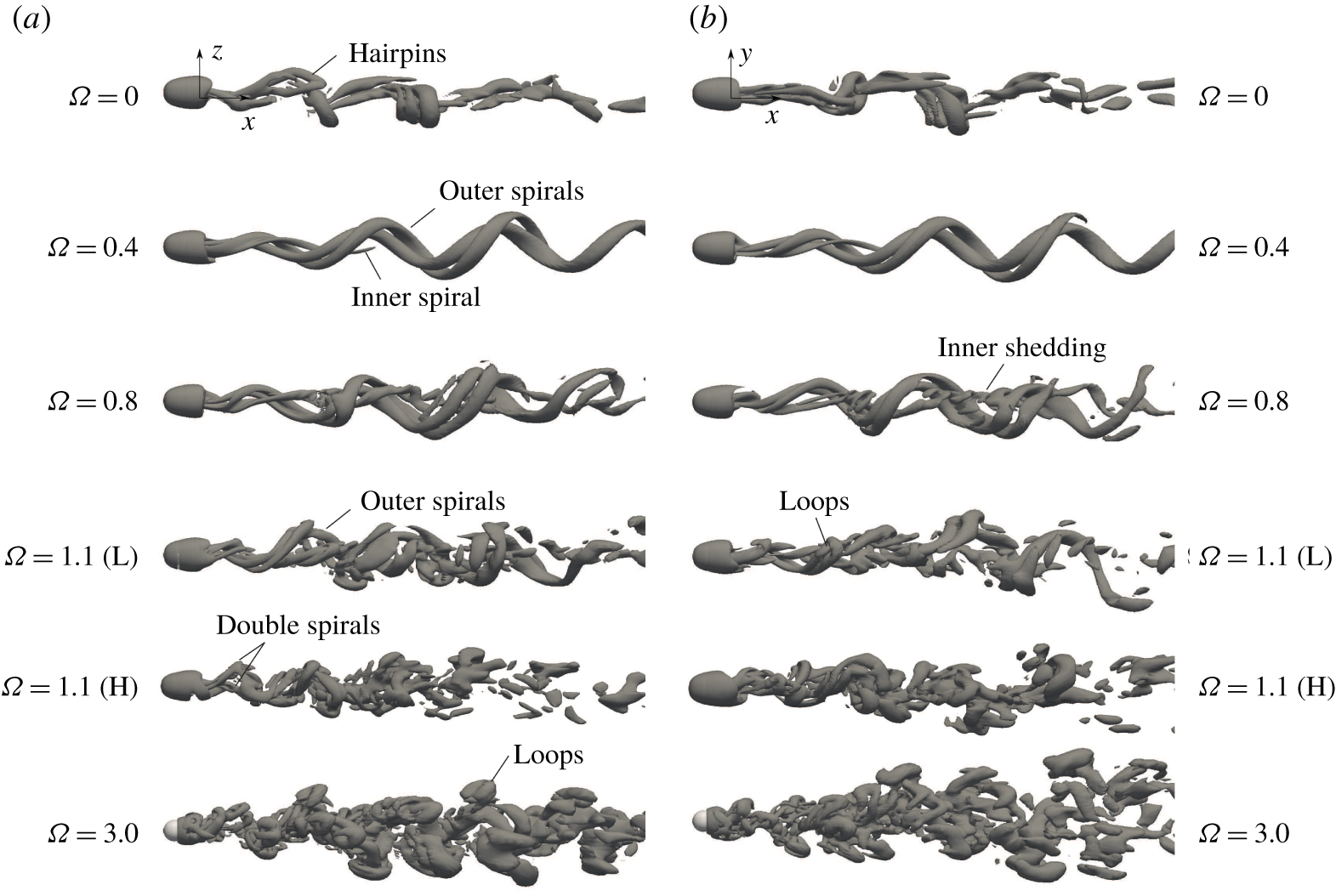
Isosurfaces of the  $Q$-quantity (
 $Q=10^{-3}$) at
 $Re=250$ and selected values of the rotation parameter
 $\unicode[STIX]{x1D6FA}$. Note that side (a) and top views (b) extend a downstream distance of
 $x=20D$ from the sphere’s rear end (corresponding movies are available in the supplemental material).

3.1 Qualitative description of flow regimes
At  $Re=250$, the flow behind the streamwise rotating sphere is unsteady for all values of
 $\unicode[STIX]{x1D6FA}>0$ investigated, and several wake regimes of increasing complexity are found as the rotation parameter increases, as shown in figure 2, where instantaneous plots of vortical structures are depicted for selected values of
 $\unicode[STIX]{x1D6FA}$ by means of isosurfaces of the
 $Q$-quantity (corresponding movies are available in the supplemental material, available at https://doi.org/10.1017/jfm.2020.342).
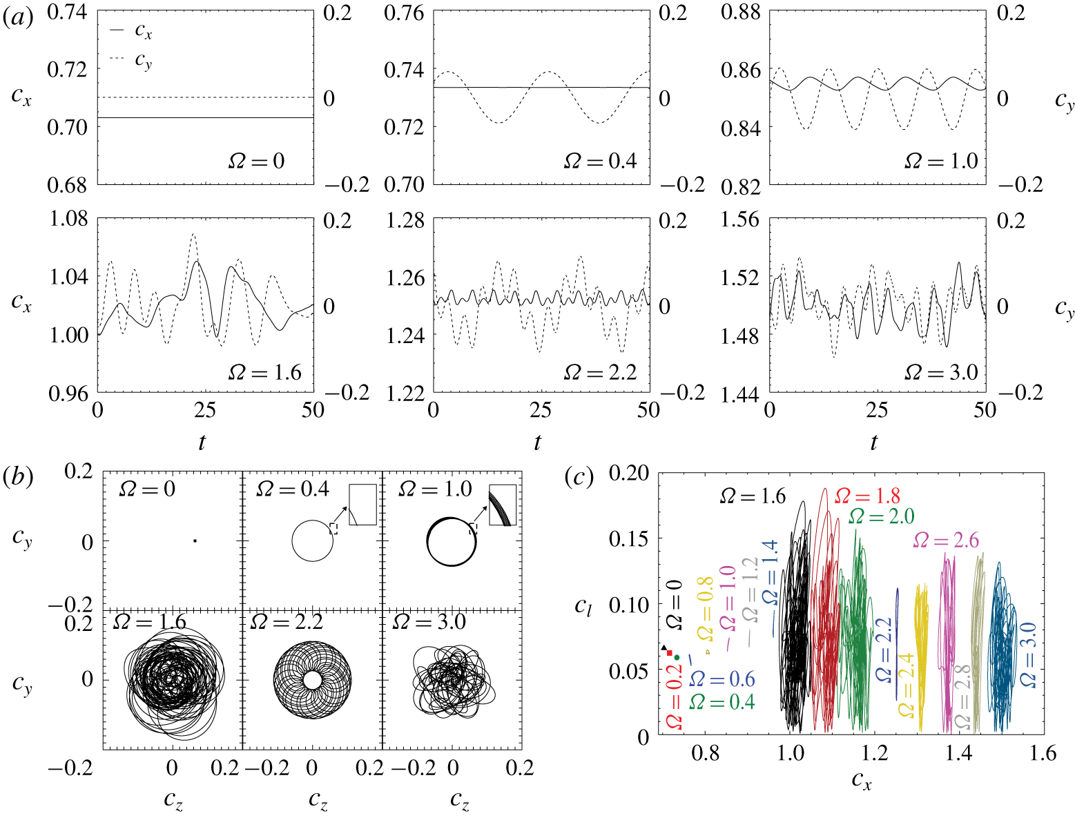
The dynamics associated to each wake regime is studied with the help of figure 3, where time histories of the drag coefficient,  $c_{x}(t)$, lift coefficient in the
 $y$-direction,
 $c_{y}(y)$, and phase diagrams (
 $c_{z},c_{y}$) and (
 $c_{l},c_{x}$) are included (note that the shown range
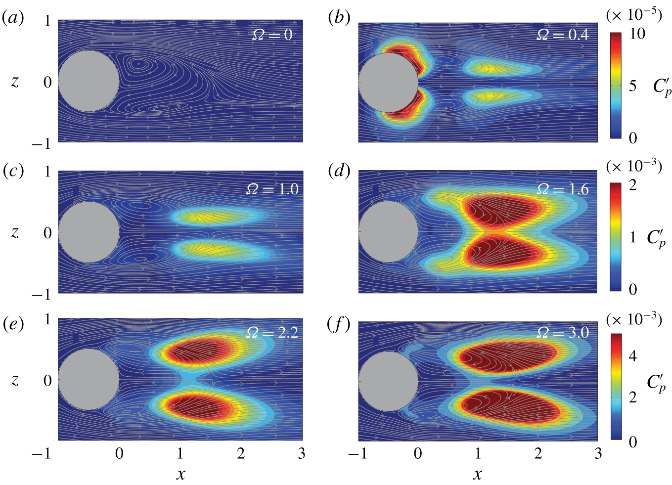
 $t\geqslant 0$ corresponds to the initial, statistically converged part of each simulation). The wake topology is further illustrated in figure 4 by means of contours of standard fluctuations of the pressure coefficient,
 $C_{p}^{\prime }$, and time-averaged velocity streamlines at
 $y=0$.
The non-rotating sphere ( $\unicode[STIX]{x1D6FA}=0$) displays a steady bifid wake with two threads of opposite axial vorticity,
 $\unicode[STIX]{x1D71B}_{x}$, which are symmetric with respect to the
 $y=0$ plane (note that the side view in figure 2 presents a conical perspective). As displayed in figure 3, such a steady state regime is characterized by constant values of drag and lift coefficients (note that
 $c_{y}=0$ due to the horizontal reflectional symmetry), and, therefore, phase diagrams
 $(c_{y},c_{z})$ and
 $(c_{l},c_{x})$ correspond to single points. A positive total lift is induced by the flow asymmetry on the vertical plane
 $z=0$ (see figure 4a).
Force coefficients for a streamwise rotating sphere at  $Re=250$. (a) Time histories of the drag coefficient,
 $c_{x}(t)$ (solid line), and lift coefficient in the
 $y$-direction,
 $c_{y}(t)$ (dashed line). (b) Phase diagrams of transversal forces (
 $c_{z},c_{y}$). (c) Phase diagrams of the total lift versus drag (
 $c_{l},c_{x}$). Insets in (b) display a zoomed part of the phase diagrams.

When the streamwise rotation is applied, the wake becomes unsteady and the reflectional symmetry is broken. For instance, at  $\unicode[STIX]{x1D6FA}=0.2$ (figure 2) the sphere rotation promotes a stronger positive vorticity thread, which displays a spiral pattern rolling in the opposite sense to that of the body swirl (this suggests that the flow dynamics may stem from the destabilization of an helical mode with azimuthal wavenumber
 $m=-1$, as highlighted by Jiménez-González, Manglano-Villamarín & Coenen Reference Jiménez-González, Manglano-Villamarín and Coenen2019), while a shroud of negative axial vorticity develops around the surface. This vortical structure is found to rotate, without any variation of shape, with a constant angular velocity whose value is smaller than the sphere’s rotation rate. This periodic or frozen regime, which has been previously identified for different rotating bodies (Kim & Choi Reference Kim and Choi2002; Jiménez-González et al. Reference Jiménez-González, Sanmiguel-Rojas, Sevilla and Martínez-Bazán2013; Pier Reference Pier2013), produces a constant value of the drag coefficient,
 $c_{x}(t)$, but periodic time histories of transverse coefficients, e.g.
 $c_{y}(t)$. This periodic rotation is identified in the phase diagram of lift components (
 $c_{y},c_{z}$) in figure 3(b), as a closed perfect circle centred at the origin (see
 $\unicode[STIX]{x1D6FA}=0.4$). Its radius indicates a constant value of
 $c_{l}$, which translates into a single point in the phase diagram (
 $c_{l},c_{x}$), as shown in figure 3(c), where it can be also observed that an increase of the value of
 $\unicode[STIX]{x1D6FA}$ leads to a growth of
 $c_{x}$. As displayed in figure 4(b), the stronger pressure fluctuations are mainly concentrated around the sphere and at the shear layer close to the downstream end of the recirculating bubble, due to the rotation of the asymmetric shroud and wavy vortex thread.
Contours of standard fluctuations of the pressure coefficient,  $C_{p}^{\prime }$, along with time-averaged velocity streamlines at
 $y=0$ for selected values of the rotation parameter
 $\unicode[STIX]{x1D6FA}$ at
 $Re=250$.

This scenario is preserved approximately until  $\unicode[STIX]{x1D6FA}=0.6$, where a new regime, characterized by the concomitant rotation of spiral structures and vortex shedding, appears, as depicted in figure 2 for
 $\unicode[STIX]{x1D6FA}=1.0$. In particular, the increase of
 $\unicode[STIX]{x1D6FA}$ strengthens the former wavy positive vorticity thread, which adopts a helical structure, being a consequence of the conservation of azimuthal momentum, which requires that fluid particles at larger values of the radial coordinate rotate more slowly. Simultaneously, there is a shedding of vortices from the shroud of negative vorticity, which are encircled by the outer spiral. Such inner vortices are convected downstream and grow into larger structures, intertwining with the helical thread.
This translates into an oscillating time history of drag coefficient  $c_{x}(t)$ (see figure 3a), and a shorter oscillation period in the lift component
 $c_{y}(t)$, due to the stronger rotation rate of the sphere. The phase diagram of lift components describes a loop which is no longer perfectly circular and features several orbits (see figure 3b insets), indicating quasi-periodic flow dynamics, i.e. the vortical structures vary their shape as they spin. Note that the total lift value fluctuates in time with a larger magnitude than the drag, thus leading to a phase diagram (
 $c_{l},c_{x}$) defined by elongated loops (figure 3c). Moreover, as
 $\unicode[STIX]{x1D6FA}$ increases, the fluctuations of
 $c_{l}$ becomes more acute than those from
 $c_{x}$ (an exception being
 $\unicode[STIX]{x1D6FA}=0.8$, as it will be later discussed), whose mean value also increases with the rotation rate.
The associated shedding intensifies the pressure fluctuations in the wake, as depicted in figure 4(c), and especially close to the rear stagnation point of the recirculation bubble.
The quasi-periodic regime prevails up to  $\unicode[STIX]{x1D6FA}=1.6$, where the wake undergoes a sudden transition to an irregular state, as depicted in figure 2. The spatial structure is more complex, featuring two irregular outer spirals (of positive vorticity
 $\unicode[STIX]{x1D71B}_{x}$) in the near wake, that become tangled as they move downstream. Additionally, there is a pair of vortices that detach from the shroud of negative
 $\unicode[STIX]{x1D71B}_{x}$ surrounding the sphere (see also pressure fluctuations close to the separation points in figure 4d) that wrap around the outer spirals while convected downstream, although they are soon dissipated. A similar double-threaded helical structure has been recently observed experimentally by Skarysz et al. (Reference Skarysz, Rokicki, Goujon-Durand and Wesfreid2018) for
 $\unicode[STIX]{x1D6FA}=1.6$. Now, fluctuating time histories of
 $c_{x}$ and
 $c_{y}$ becomes irregular (see figure 3a), leading to complex phase diagrams of (
 $c_{y},c_{z}$) and (
 $c_{l},c_{x}$) in figure 3(b,c), anticipating the existence of multiple frequency components. In general, the vortical structures of this regime feature a higher eccentricity than those observed earlier, as depicted in figure 4(d), on account of the larger centrifugal driving force induced by
 $\unicode[STIX]{x1D6FA}$. As a consequence, the amplitude of lift components and total lift are considerably larger than those reported for the previous regime (see figure 3b,c). In view of such features, we will sometimes refer to such a regime as high-helical irregular, to identify the irregular swirl and shedding of double spiral structures.
As the rotation rate increases above  $\unicode[STIX]{x1D6FA}=2$, the wake arranges itself into a more coherent double helical structure in the near wake, as observed in figure 2 for
 $\unicode[STIX]{x1D6FA}=2.2$. The wake rotation now features a quasi-periodic time history of the lift component
 $c_{y}$ and a fluctuating drag
 $c_{x}$ (figure 3a). A closer analysis of
 $c_{y}$ shows that there are two characteristic oscillating periods, which, as it will be later detailed, are related to the swirl of two different spatial structures in the wake, namely single and double helices, with azimuthal symmetries (wavenumbers)
 $m=-1$ (
 $m_{1}$) and
 $-2$ (
 $m_{2}$). Such a new high-helical quasi-periodic regime is clearly observable at the phase diagrams depicted in figure 3(b,c), and is associated to stronger pressure fluctuations (see figure 4e), whose loci are less aligned with the flow streamlines, on account of the larger radial inclination of spiral threads.
Finally, for  $\unicode[STIX]{x1D6FA}\geqslant 2.4$, the wake becomes irregular again, and the higher swirl of the flow induces stronger double-threaded helices in the near wake that tilt and connect to form vortex loops in different directions, as observed in figure 2 for
 $\unicode[STIX]{x1D6FA}=3$.
Such vortex loops rotate with the vortical structure as they move downstream, changing progressively their orientation, before dissipating in the far wake. The irregular regime presents uneven time histories of force coefficients, as displayed in figure 3(a), where an important modulation of the amplitude and multiple frequencies are distinguishable in  $c_{x}$ and
 $c_{y}$. As a consequence, the phase diagram of lift components
 $(c_{y},c_{z})$ becomes entangled (figure 3b). Interestingly, the radial extension of such a phase portrait is smaller than that corresponding to the irregular regime reported for
 $\unicode[STIX]{x1D6FA}=1.6$, and so is the largest fluctuating value of the total lift, as shown in figure 3(c). In addition, the
 $(c_{l},c_{x})$ diagrams also show that the fluctuations of
 $c_{x}$ become progressively larger within this regime as
 $\unicode[STIX]{x1D6FA}$ increases, leading to wider phase diagrams. This is an indication of the fostering of the shedding process, associated to important overall pressure changes in the rear part of the sphere, as figure 4(f) depicts. There it can also be estimated that the time-averaged separation angle,
 $\unicode[STIX]{x1D6F7}_{s}$, decreases with growing rotation since it acts by lowering the pressure on the equator, thus creating an increasingly adverse gradient that fosters the flow separation.
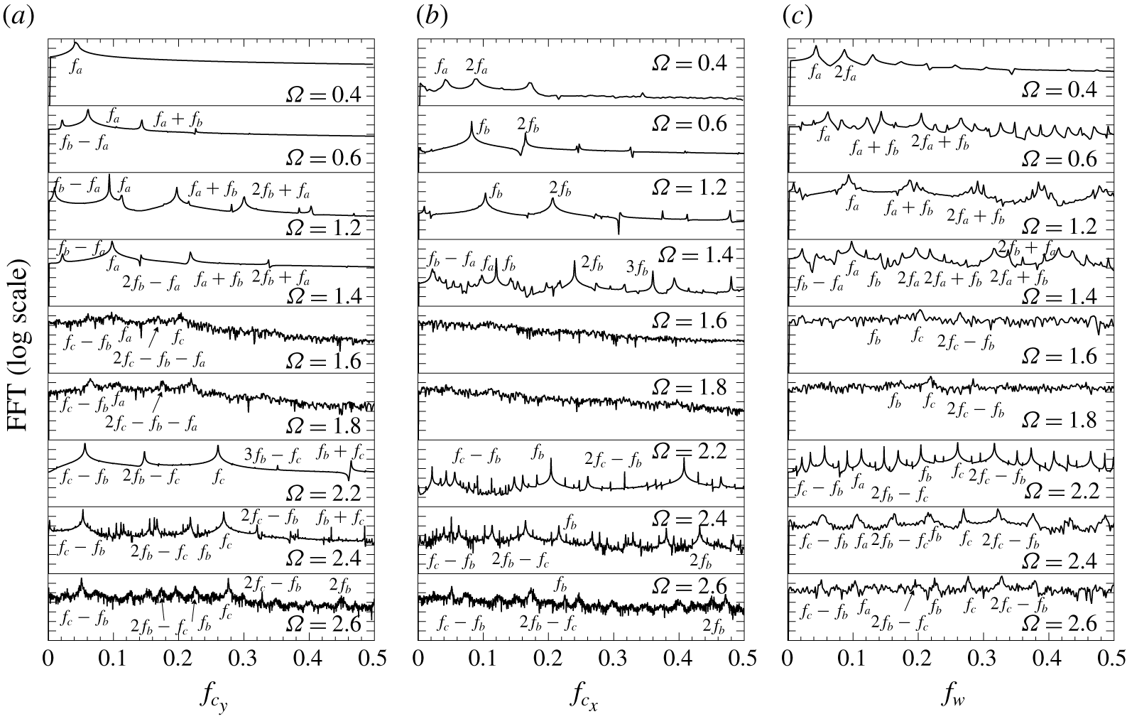
Fast Fourier transform spectra, listing the main frequency components, for different rotation parameters,  $\unicode[STIX]{x1D6FA}$, at
 $Re=250$ corresponding to the (a)
 $y$-axis lift coefficient,
 $c_{y}^{\prime }=c_{y}-C_{y}$, (b) drag coefficient,
 $c_{x}^{\prime }=c_{x}-C_{x}$, and the (c) azimuthal velocity
 $w^{\prime }=w-W$ at
 $(x,y,z)=(2,0.5,0)$. The same amplitude logarithmic scale is used for all fast Fourier transform spectra, including decades that range from
 $10^{0}$ to
 $10^{-6}$.

3.2 Frequency analysis
We next further analyse the flow regimes and transitions in terms of frequency components from spectra obtained by computing the fast Fourier transform (FFT) of time fluctuating values of force coefficients,  $c_{y}^{\prime }=c_{y}-C_{y}$ and
 $c_{x}^{\prime }=c_{x}-C_{x}$, and the azimuthal velocity,
 $w^{\prime }=w-W$, at the selected location
 $(x,y,z)=(2,0.5,0)$, which displays the largest amplitudes of fluctuating components (not shown) in comparison with other axial and radial positions. Corresponding FFT spectra of
 $c_{y}^{\prime }$,
 $c_{x}^{\prime }$ and
 $w^{\prime }$ for selected values of
 $\unicode[STIX]{x1D6FA}$ are included in figure 5, where the main components of frequency are identified and labelled to enlighten (and simplify) the discussion on the flow transitions. Note also that the same logarithmic scale is used for all FFT spectra aiming at establishing a quantitative comparison of amplitudes associated to different frequency components.
For the non-rotating sphere ( $\unicode[STIX]{x1D6FA}=0$), the wake is steady and, therefore, no FFT spectrum is included. At
 $\unicode[STIX]{x1D6FA}=0.4$, the signal of
 $c_{y}$, shown in figure 3(a), is periodic according to its FFT, with a fundamental frequency
 $f_{a}$, which is related to the rate of rotation of the wake. However, the harmonic
 $2f_{a}$ develops at the near wake, as observed in the spectrum of
 $w^{\prime }$, although its magnitude is weak in comparison with the main peak. Interestingly, if the sphere’s rotation frequency is denoted as
 $f_{r}$, the ratio
 $f_{a}/f_{r}\simeq \frac{1}{3}$, which agrees well with previously reported values by Pier (Reference Pier2013) and Skarysz et al. (Reference Skarysz, Rokicki, Goujon-Durand and Wesfreid2018) for low
 $\unicode[STIX]{x1D6FA}$.
At  $\unicode[STIX]{x1D6FA}=0.6$, a new frequency, labelled
 $f_{b}$, emerges in the spectrum of
 $c_{x}^{\prime }$ (figure 5b). As a consequence, new peaks resulting from the interaction of these two incommensurate frequencies
 $f_{a}$ and
 $f_{b}$, arise in the spectra of
 $c_{y}^{\prime }$ and
 $w^{\prime }$ (figure 5a,c), leading to the previously described quasi-periodic regime. In particular, modulations in the amplitude of
 $c_{y}(t)$ in figure 3(a) and the orbit of the phase diagram
 $(c_{y},c_{x})$ in figure 3(b) occur at a frequency
 $f_{a}+f_{b}$, although they are barely discernible on account of the low magnitude of such frequency components shown in the FFT of
 $c_{y}^{\prime }$.
As the rotation rate  $\unicode[STIX]{x1D6FA}$ increases, harmonics and nonlinear interactions between the previous frequencies produce new peaks of moderate amplitude (see, e.g.
 $f_{b}-f_{a}$,
 $f_{a}+f_{b}$,
 $2f_{b}+f_{a}$ or
 $2f_{b}-f_{a}$ in the spectra for
 $\unicode[STIX]{x1D6FA}=1.2$ and 1.4). The frequency
 $f_{a}$ increases with
 $\unicode[STIX]{x1D6FA}$ which indicates an acceleration of the wake rotation, although such growth becomes progressively less important within the quasi-periodic regime, leading to a rate
 $f_{a}/f_{r}$ that decreases monotonously.
As described earlier, this quasi-periodic regime prevails at the wake until  $\unicode[STIX]{x1D6FA}=1.6$, when the high-helical irregular regime sets in (see figure 2). The frequency analysis shows that, at
 $\unicode[STIX]{x1D6FA}=1.6$, some of the former fundamental frequency components and nonlinear interactions are distinguishable in the spectra of
 $c_{y}^{\prime }$ and
 $w^{\prime }$ as broader peaks (no clear peaks are observed for the
 $c_{x}^{\prime }$ spectrum), being an indication of richer dynamics, compatible with a chaotic wake behaviour (an observation which will be further discussed in § 7). However, the most interesting feature is the development of a third incommensurate frequency component, denoted
 $f_{c}$, that presents the largest amplitude at the wake, so that an irregular regime is related to the confluence of three incommensurate frequencies.
In addition, the combined frequency  $2f_{c}-f_{b}$ stands out in the
 $w^{\prime }$ spectrum (figure 5c), which, as it will be detailed in the following section, is associated to the swirl of a double spiral structure which develops in the near wake.
Fast Fourier transform spectra of axial and transverse velocities,  $u^{\prime }=u-U$ and
 $w^{\prime }=w-W$, and pressure,
 $p^{\prime }=p-P$, at downstream axial locations,
 $x\leqslant 10$, and radial locations
 $r=[0,0.5]$ for the selected value of
 $\unicode[STIX]{x1D6FA}=1.6$ and
 $Re=250$.

The irregular state evolves as  $\unicode[STIX]{x1D6FA}$ increases, until
 $\unicode[STIX]{x1D6FA}=2.2$, where spectra display a new quasi-periodic behaviour related to a synchronization regime, dominated by frequency
 $f_{c}$ and its quadratic interactions with
 $f_{b}$ (see figure 5a). In particular, modulations in amplitude of
 $c_{y}^{\prime }(t)$ in figure 3(a) (and in the orbit of the lift diagram) take place with a frequency
 $f_{c}-f_{b}$. In addition, the amplitude of peaks is considerably smaller for
 $c_{x}^{\prime }$, indicating weaker fluctuating dynamics, as observed in the
 $(c_{y},c_{x})$ diagram (figure 3c). Interestingly, at the near wake, the dynamics is governed by
 $2f_{c}-f_{b}$, as displayed in the
 $w^{\prime }$ spectrum (figure 5c).
Finally, for  $\unicode[STIX]{x1D6FA}\geqslant 2.4$, the same dominating frequency components are present in the spectra, although now multiple additional peaks develop, all of them featuring broader bases. The latter indicates again a transition towards the irregular regime.
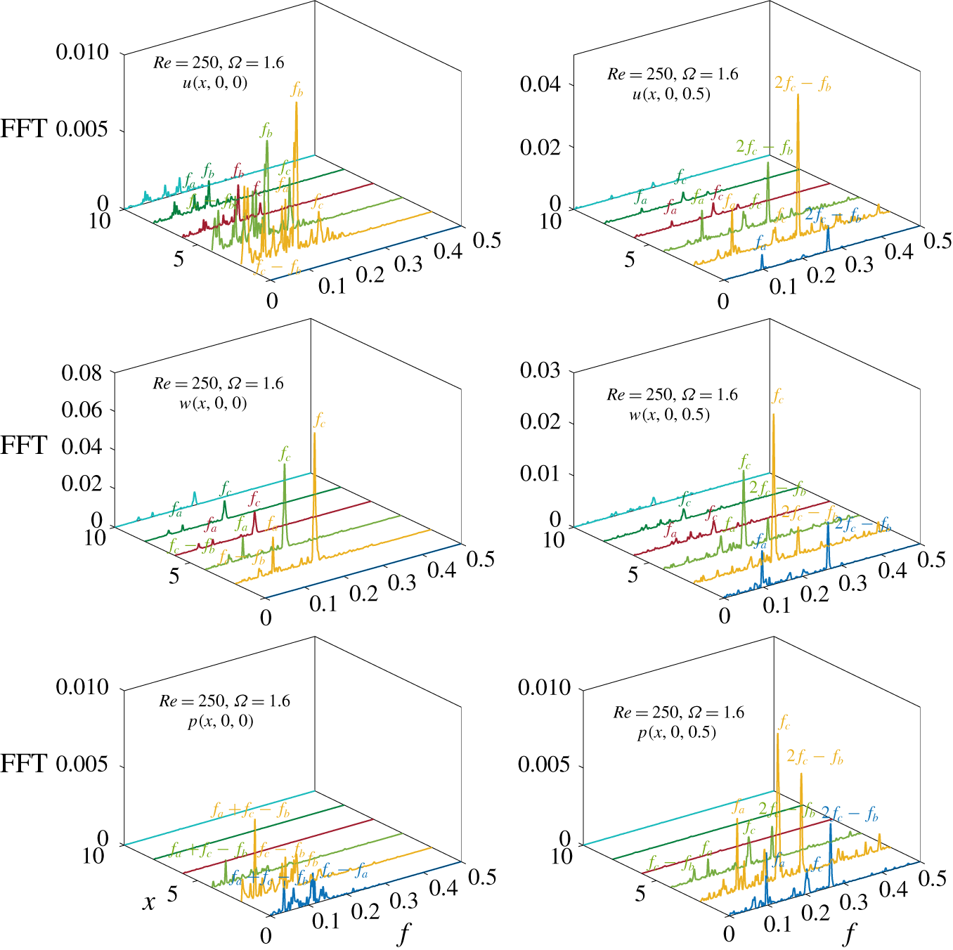
To analyse the axial extent, spatial prevalence and to infer the azimuthal nature of the different features associated with the different frequencies in the near wake, we display in figure 6 the FFT spectra of axial and transverse velocities,  $u^{\prime }=u-U$ and
 $w^{\prime }=w-W$, and pressure,
 $p^{\prime }=p-P$, at downstream axial,
 $x\leqslant 10$, and radial locations
 $r=[0,0.5]$ for the selected value of
 $\unicode[STIX]{x1D6FA}=1.6$, where the three incommensurate frequencies
 $f_{a}$,
 $f_{b}$ and
 $f_{c}$, and the derived frequency
 $2f_{c}-f_{b}$ are present. The energy of such frequencies decays in general for
 $x\geqslant 6$, and peaks associated to
 $f_{c}$ and
 $2f_{c}-f_{b}$ are particularly energetic for all variables. In particular,
 $2f_{c}-f_{b}$ stands out in FFT spectra taken at
 $r=0.5$ and
 $x\leqslant 4$, indicating that the associated structures are mainly near wake structures. The frequency
 $f_{c}$ features the largest spectral magnitude at
 $r=0.5$ and
 $r=0$ for the transverse velocity, congruent with a helical pattern extending up to
 $x=10$. A similar picture can be observed for the component
 $f_{a}$, associated to the rotating helical structures stemming from the periodic regime, however, the corresponding peaks are less energetic at this level of
 $\unicode[STIX]{x1D6FA}$. Finally, the peak
 $f_{b}$ is only observable at
 $r=0$ for spectra of the pressure
 $p^{\prime }$ and axial velocity
 $u^{\prime }$, extending until
 $x=10$. Thus, the associated phenomenon mostly occurs at a centred location, as shown by the shedding in figure 2 for
 $\unicode[STIX]{x1D6FA}=1$.
3.3 Flow decomposition
3.3.1 Higher-order dynamic mode decomposition
At this point, a deeper analysis of vortical structures is required to better identify the wake dynamics and nature of the different flow regimes. To that aim, flow decomposition techniques will be employed in order to infer the spatial symmetries that dominate each regime, and structures associated to each component frequency. First, a higher-order dynamic mode decomposition (HODMD) technique (Le Clainche & Vega Reference Le Clainche and Vega2017a) has been employed to extract dynamic modes linked to particular frequencies observed in figure 5 (see appendix B for details). The analysis is performed with snapshots of the velocity field taken at  $x=2$,
 $\boldsymbol{u}(x=2,y,z,t)$, where the largest spectral amplitudes are found, as shown in figure 6.
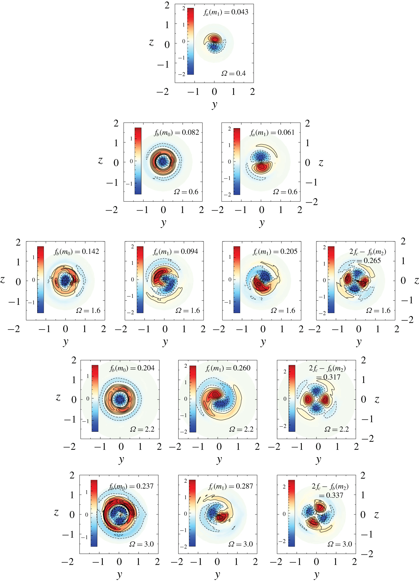
Results for  $Re=250$ are summarized in figure 7, where spatial structures are identified by means of contours of the real part of the normalized axial vorticity
 $\mathbb{R}(\unicode[STIX]{x1D71B}_{x})$ (using the mode infinity norm
 $\Vert \boldsymbol{u}\Vert _{\infty }$), along with their associated frequency, for selected values of the rotation parameter
 $\unicode[STIX]{x1D6FA}$. To simplify the analysis, only characteristic modes featuring the largest amplitudes are included (an example of the spectral complexity obtained can be found in appendix B).
Contours of the normalized axial vorticity  $\unicode[STIX]{x1D71B}_{x}$ (real part) for the most representative modes identified through HODMD analysis for selected values of
 $\unicode[STIX]{x1D6FA}$ at
 $Re=250$. Modes are arranged from left to right in increasing order of azimuthal wavenumber.

Although not shown, the non-rotating sphere’s wake is characterized by a steady (frequency  $f=0$) mode displaying a dipole of axial vorticity, compatible with an azimuthal symmetry with wavenumber
 $m=1$ (
 $m_{1}$). With rotation, the mode becomes unsteady and a periodic regime emerges in the wake.
At  $\unicode[STIX]{x1D6FA}=0.4$, the mode presents a frequency
 $f(m_{1})=0.043$ which corresponds to the peak
 $f_{a}$ identified in figure 5(c). As
 $\unicode[STIX]{x1D6FA}$ increases up to a value of 0.6, a new fundamental frequency
 $f_{b}$ was identified in the spectra of figure 5 and related to the periodic shedding of vortices, leading to a new unsteady quasi-periodic regime in the wake. When the dynamic modes are computed, aside from the former
 $m_{1}$ structure associated to
 $f=0.061\equiv f_{a}$, a new energetic mode is found for
 $f(m_{0})=0.082$. This frequency corresponds to the peak
 $f_{b}$ of figure 5, which identifies the periodic shedding observable in figure 2 at
 $\unicode[STIX]{x1D6FA}=1$. Interestingly, the mode shows a nearly axisymmetric distribution of vorticity, featuring an outer ring of positive vorticity and an inner core of negative vorticity. Such topology might be related to an axisymmetric pulsation from the excitation of a
 $m=0$ mode that leads to the inner shedding of vortices, in line with the observations made from figure 2.
For  $\unicode[STIX]{x1D6FA}=1.6$, a new irregular regime sets in the wake, characterized by a double-helical flow structure, as displayed in figure 2. This double-threaded wake may be an indication of the destabilization of a mode with azimuthal wavenumber
 $m=2$ (
 $m_{2}$), as occurs for generic swirling flows at high values of flow rotation (see, e.g. Ruith et al. Reference Ruith, Chen, Meiburg and Maxworthy2003). In particular, the HODMD analysis reveals that the most energetic mode corresponds to an
 $m_{1}$ symmetry, which is qualitatively different to the dipole identified at lower rates of rotation, and resembles the Yin-Yang mode (Auguste, Fabre & Magnaudet Reference Auguste, Fabre and Magnaudet2010) identified experimentally by Skarysz et al. (Reference Skarysz, Rokicki, Goujon-Durand and Wesfreid2018), its frequency being
 $f(m_{1})\equiv f_{c}=0.205$. Additionally, the second largest amplitude is related to
 $f=0.262$, which corresponds to the frequency component
 $2f_{c}-f_{b}$ identified in figure 5, and displayed a quadrupole of vorticity compatible with an
 $m=2$ symmetry. Such azimuthal symmetry is the outcome of the interaction of harmonic
 $2f_{c}$ (
 $2\cdot m_{1}$) and
 $f_{b}$ (
 $m_{0}$), and would be responsible for the double-helical structure observed in figure 2. Moreover, as in the previous quasi-periodic regime, the modes associated to
 $f_{a}=0.093$ (
 $m_{1}$ symmetry) and
 $f_{b}=0.141$ (
 $m_{0}$ symmetry) are also identified at the wake, although their corresponding growth rates are small in comparison with those of
 $f_{c}$ and
 $2f_{c}-f_{b}$, which mainly govern the flow dynamics.
At  $\unicode[STIX]{x1D6FA}=2.2$, a more organized wake state appears, through a synchronization of the wake at selected frequencies
 $2f_{c}-f_{b}$,
 $f_{c}$ and
 $f_{b}$, and the corresponding modes display a better spatial resolution. The same picture is obtained for
 $\unicode[STIX]{x1D6FA}>2.2$ within the irregular regime, although modes feature a more irregular topology.
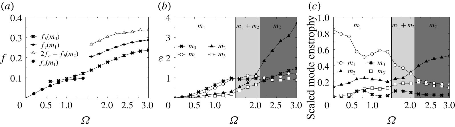
A summary of the evolution with  $\unicode[STIX]{x1D6FA}$ of frequencies associated to previously described most energetic modes is shown in figure 8(a). As observed, the wake rotation frequency
 $f_{a}$ grows at low rotation rates to reach a constant value at
 $\unicode[STIX]{x1D6FA}\simeq 1.2$. The shedding frequency
 $f_{b}$ emerges around
 $\unicode[STIX]{x1D6FA}=0.6$, causing the transition towards the quasi-periodic regime, and grows monotonously with
 $\unicode[STIX]{x1D6FA}$ within the range investigated. The abrupt transition to the irregular regime at
 $\unicode[STIX]{x1D6FA}=1.6$ is produced by the existence of a new fundamental frequency component,
 $f_{c}$, and its quadratic interaction
 $2f_{c}-f_{b}$, as sketched in figure 8(a), where the trend has also been plotted for the sake of comparison. As expected, the dynamics is sped up with rotation, giving growing trends of
 $f_{b}$ and
 $f_{c}$ within the range
 $1.6\leqslant \unicode[STIX]{x1D6FA}\leqslant 3$. On the other hand, the apparent mode azimuthal wavenumber
 $m$ is also listed for each frequency component in figure 8(a) to qualitatively indicate the azimuthal symmetries present for each regime. Below
 $\unicode[STIX]{x1D6FA}=1.6$ the flow is mainly governed by an
 $m_{1}$ symmetry, while above this threshold there is a coexistence of
 $m_{1}$ and
 $m_{2}$ structures.
Flow decomposition at  $Re=250$: evolution with
 $\unicode[STIX]{x1D6FA}$ of (a) characteristic frequencies corresponding to dominant modes; (b) enstrophy,
 $\unicode[STIX]{x1D700}(m)$, for the most energetic azimuthal symmetries (FAD); and (c) relative contribution to total enstrophy for symmetries
 $m=0,1,2$ and 3 (FAD). The vertical lines in (b,c) distinguish regimes with different dominant azimuthal symmetries.

3.3.2 Fourier azimuthal decomposition
The estimation of the total energy contribution of each azimuthal symmetry using the HODMD would require us to compute a large number of modes. Hence, the competition between azimuthal symmetries is better analysed using a Fourier azimuthal decomposition (FAD) of the instantaneous streamwise vorticity field,  $\unicode[STIX]{x1D71B}_{x}(x,y,z,t)$, at the same downstream location
 $x=2$. We refer the reader to appendix B for technical details of this decomposition. The total streamwise enstrophy is computed for each azimuthal symmetry
 $m$ as
 $\unicode[STIX]{x1D700}(m)=(1/A)\int \unicode[STIX]{x1D701}(m)^{2}\,\text{d}A$, where
 $\unicode[STIX]{x1D701}(m)$ is computed according to (B 2) and
 $A$ represents the area of integration (a circle of radius
 $r=2$). The enstrophy quantifies the flow energy associated to each azimuthal symmetry and, therefore, provides a good estimation of the dominant flow structures at each
 $\unicode[STIX]{x1D6FA}$. The evolutions of
 $\unicode[STIX]{x1D700}(m)$ with
 $\unicode[STIX]{x1D6FA}$ for the first four modes
 $m\in [0,3]$ are depicted in figure 8(b). The energy contained in such modes represents more than
 $95\,\%$ of the total energy for all values of
 $\unicode[STIX]{x1D6FA}$ investigated.
First, it is observed that, for  $\unicode[STIX]{x1D6FA}\leqslant 1.4$,
 $m=1$ (
 $m_{1}$) and
 $m=0$ (
 $m_{0}$) symmetries are the most energetic at the wake. In particular, the enstrophy of mode
 $m_{0}$ grows monotonously with
 $\unicode[STIX]{x1D6FA}$ until it reaches a saturated value around 1.4, in line with the experimental results of Skarysz et al. (Reference Skarysz, Rokicki, Goujon-Durand and Wesfreid2018). Therefore, the initial growth in
 $\unicode[STIX]{x1D700}(m_{0})$ during the periodic and quasi-periodic regimes can be attributed to the linear addition of cyclonic vorticity due to the rotation of the sphere. In addition, at
 $\unicode[STIX]{x1D6FA}=0$ the
 $m_{1}$ mode dominates as a result of the presence of the SS regime at the wake behind the non-rotating sphere for
 $Re=250>Re_{c1}$. As the rotation is applied, at
 $\unicode[STIX]{x1D6FA}=0.2$ there is a slight decrease in the energy of
 $m_{1}$, which barely displays the same energy as
 $m_{0}$. As a consequence, the flow regime adopts a nearly axisymmetric configuration, as shown in figure 2, characterized by a wavy, slightly eccentric, thread of positive vorticity, although the axisymmetry is not completely retrieved at the wake. From there on, the energy of mode
 $m_{1}$ grows monotonously until
 $\unicode[STIX]{x1D6FA}=1.6$, from where it starts to stagnate.
Around  $\unicode[STIX]{x1D6FA}=1.6$, the enstrophy associated to
 $m=2$,
 $\unicode[STIX]{x1D700}(m_{2})$, starts to grow rapidly and becomes the dominant symmetry at
 $\unicode[STIX]{x1D6FA}=2$. Such an abrupt change in the trend of
 $\unicode[STIX]{x1D700}(m_{2})$ is related to the excitation of a new dynamic mode associated to the frequency
 $f_{m_{2}}\equiv 2f_{c}+f_{b}$, as previously described (see figures 5 and 7).
In particular, the new linear trend displayed by  $\unicode[STIX]{x1D700}(m_{2})$ allows a first estimation of the threshold of instability for the mode of
 $f_{m_{2}}$ (figure 7), by means of Landau’s model,
 $E\simeq K\cdot (\unicode[STIX]{x1D6FA}-\unicode[STIX]{x1D6FA}_{cr})$, giving a critical value of
 $\unicode[STIX]{x1D6FA}_{cr}\simeq 1.57$ (note that a similar experimental value was recently identified by Skarysz et al. (Reference Skarysz, Rokicki, Goujon-Durand and Wesfreid2018) for the transition between
 $m_{1}$ and
 $m_{2}$).
Therefore, the periodic and quasi-periodic flows below 1.6 are governed by  $m_{1}$ (and
 $m_{0}$), while the irregular regime observed for
 $1.6\leqslant \unicode[STIX]{x1D6FA}\leqslant 2$ is the outcome of the coexistence of
 $m_{0}$,
 $m_{1}$ and
 $m_{2}$ modes. Finally, the abrupt destabilization of an
 $m_{2}$ mode above
 $\unicode[STIX]{x1D6FA}=2$ leads to the complex three-dimensional double-helical topology of the wake shown in figure 2. Such qualitative scenarios are sketched in figure 8(b) by means of shaded ranges.
A second FAD analysis is performed by taking fluctuating values of axial vorticity (without any mean) in (B 1), i.e.  $\unicode[STIX]{x1D71B}_{x}^{\prime }(t)=\unicode[STIX]{x1D71B}_{x}(t)-\unicode[STIX]{x1D6F1}_{x}$, to get rid of the steady cyclonic vorticity provided by the sphere’s rotation, and to evaluate the competition between
 $m_{1}$ and
 $m_{2}$ structures. In that sense, figure 8(c) depicts the contribution of modes
 $m_{1}$ and
 $m_{2}$ to the total enstrophy at each value of
 $\unicode[STIX]{x1D6FA}$, where the fluctuating axisymmetric pulsation with
 $m_{0}$ has been also included. As observed, such modes contain more than
 $90\,\%$ of the total energy for
 $\unicode[STIX]{x1D6FA}\leqslant 1.6$, although their total contribution reduces at higher rotation rates due to the excitation of modes of larger
 $m$ (at
 $\unicode[STIX]{x1D6FA}=3$, their energy amounts to
 $75\,\%$ approximately). In particular, from
 $\unicode[STIX]{x1D6FA}=1.6$ onwards the contribution of
 $m_{1}$ starts to decrease linearly while that of
 $m_{2}$ grows and becomes dominant at
 $\unicode[STIX]{x1D6FA}=2$. Interestingly, the axisymmetric
 $m_{0}$ unsteady contribution rises around
 $\unicode[STIX]{x1D6FA}=0.8$ and
 $1.6$, coinciding respectively with the onset of the corresponding quasi-periodic (
 $m_{1}$) and irregular
 $m_{2}$ regimes. Note that such events imply width changes in the
 $(c_{l},c_{x})$ diagrams of figure 3(c).
4 Flow regimes behind a streamwise rotating sphere at Re $=$ 500

Isosurfaces of the  $Q$-quantity (
 $Q=10^{-2}$) at
 $Re=500$ and selected values of the rotation parameter
 $\unicode[STIX]{x1D6FA}$. Note that side (a) and top views (b) extend a downstream distance of
 $x=20D$ from the sphere’s rear end (corresponding movies are available in the supplemental material). Tags L and H respectively denote the two different states of low and high drag introduced in the text.

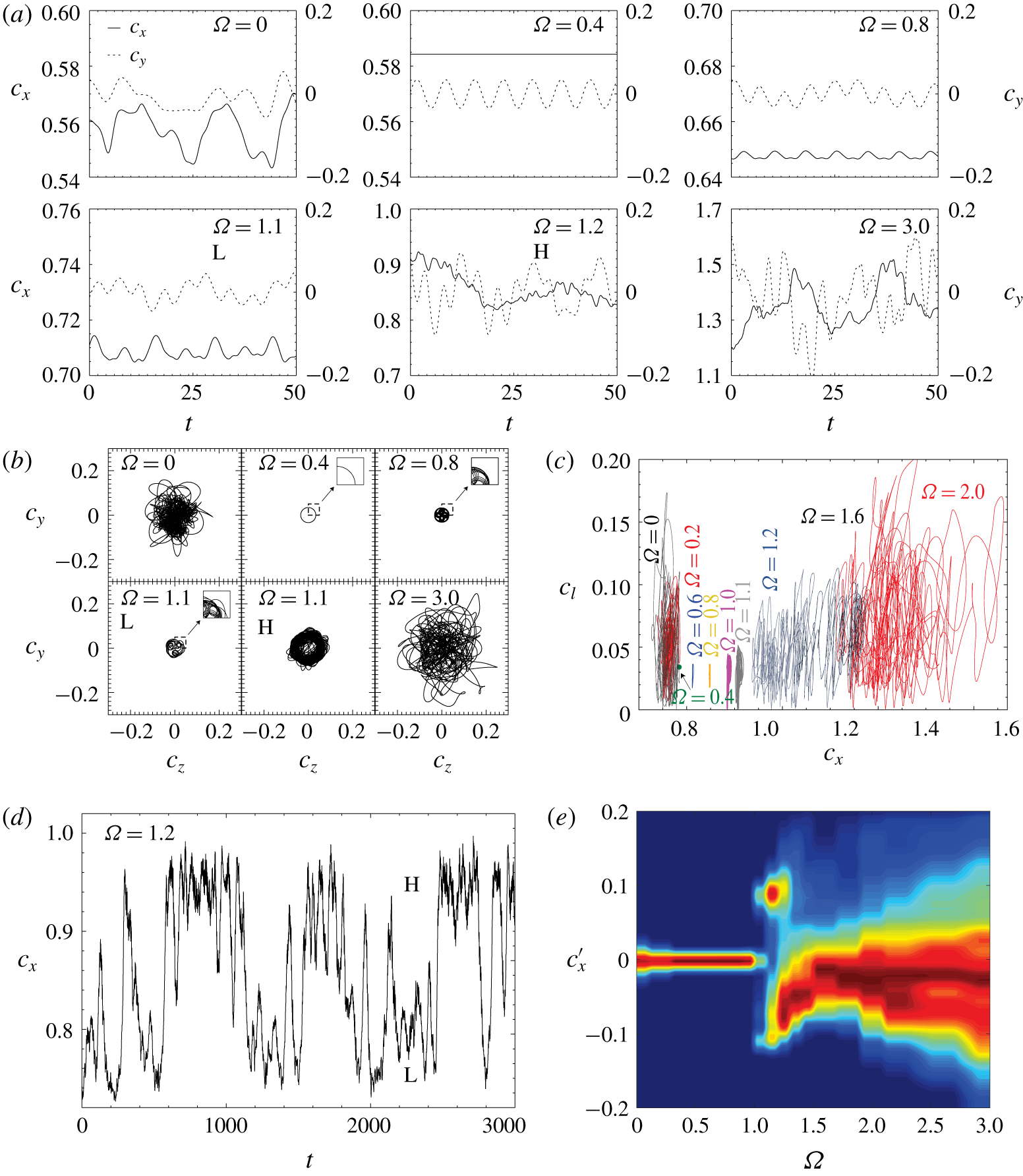
Force coefficients at  $Re=500$: (a) time histories of the drag coefficient,
 $c_{x}(t)$ (solid line), and the lift coefficient in the
 $y$-direction,
 $c_{y}(t)$ (dashed line); (b) phase diagrams of transversal forces (
 $c_{z},c_{y}$); and (c) phase diagrams of the total lift versus drag (
 $c_{l},c_{x}$). (d) Time-evolution of
 $c_{x}$ at
 $\unicode[STIX]{x1D6FA}=1.2$ and (e) contours of the probability density function (PDF) of
 $c_{x}^{\prime }=c_{x}-C_{x}$ for all rotation parameter values,
 $\unicode[STIX]{x1D6FA}$, at
 $Re=500$. Note that each PDF is normalized by its corresponding maximum value at each
 $\unicode[STIX]{x1D6FA}$, i.e. PDF (
 $c_{x}^{\prime }$) ranges from 0 (blue) to 1 (red). Insets in (b) display a zoomed part of the phase diagrams, while the tags L and H in (d) respectively denote the low and high drag states.

4.1 Qualitative description of flow regimes
The different qualitative wake regimes encountered for  $Re=500$ and increasing
 $\unicode[STIX]{x1D6FA}$ are summarized in figure 9, where instantaneous plots of vortical structures are displayed using isosurfaces of the
 $Q$-quantity, and in figure 10, which includes time histories of
 $c_{x}(t)$ and
 $c_{y}(t)$, and corresponding phase diagrams
 $(c_{y},c_{z})$ and
 $(c_{l},c_{x})$ for selected values of
 $\unicode[STIX]{x1D6FA}$. Note that, unlike
 $Re=250$, a level of
 $Q=10^{-2}$ has been set in figure 9 since a higher threshold is required to display coherent and neat topologies (the larger axial shear induced by the stronger axial velocity gradients increases the magnitude of the rotation tensor and then larger values of
 $Q$ are found at the wake as
 $Re$ grows).
As reported by Tomboulides & Orszag (Reference Tomboulides and Orszag2000), at  $\unicode[STIX]{x1D6FA}=0$ the wake is characterized by an irregular hairpin vortex-shedding, featuring an uneven azimuthal rotation of the separation point at the sphere’s rear. Thus, the hairpin vortices observed in figure 9 display different orientations at the wake and there is no trace of the planar symmetry seen at
 $Re=250$. The irregular nature is also observed in the time histories of
 $c_{y}(t)$ and
 $c_{x}(t)$ (see figure 10a), and corresponding phase diagrams
 $(c_{y},c_{z})$ and
 $(c_{l},c_{x})$ in figure 10(b,c).
With rotation, the irregular shedding regime remains present up to  $\unicode[STIX]{x1D6FA}=0.4$, where a sudden transition towards a periodic regime takes place. As observed in figure 9, the wake arranges itself into a coherent helical structure displaying two counter-rotating threads (configuring the outer spiral) and an inner near wake spiral of negative axial vorticity, which, in fact, is attached to the main negative thread. Such structures rotate together in a frozen manner, which translates into a steady drag time history,
 $c_{x}(t)$, and periodic lift components,
 $c_{y}(t)$, as displayed in figure 10(a). As a consequence, the phase diagram of
 $(c_{y},c_{z})$ is represented by a perfect circular orbit (see figure 10b), while the corresponding phase diagram
 $(c_{l},c_{x})$ is a point (see figure 10c). Interestingly, the more organized nature of the wake and the constant eccentricity of near wake structures leads to a smaller value of the mean total lift than that associated to the irregular shedding regime, as seen in figure 10(c). Such a regime is equivalent to the high-frequency or spiral frozen regimes respectively identified by Pier (Reference Pier2013) or Jiménez-González et al. (Reference Jiménez-González, Sanmiguel-Rojas, Sevilla and Martínez-Bazán2013).
The spiral frozen regime is soon disrupted when  $\unicode[STIX]{x1D6FA}$ increases above 0.6. In particular, the inner near wake spiral elongates and is torn apart downstream due to the induced shear from the outer double spiral structure, which now becomes less coherent, as observed for
 $\unicode[STIX]{x1D6FA}=0.8$ (figure 9). As shown in figure 10, such a wake regime is characterized by an oscillating time history of
 $c_{x}(t)$ and low frequency modulations in the lift
 $y$-component signal,
 $c_{y}(t)$, which is no longer periodic. Thus, the phase diagram
 $(c_{y},c_{z})$ presents a quasi-periodic orbit, which leads to a fluctuating behaviour of the total lift
 $c_{l}(t)$ (see figure 10c).
At  $\unicode[STIX]{x1D6FA}=1.1$ the wake displays a more irregular structure, as observed in figure 9, and the shedding of vortices of smaller scale from the inner vortical structure is strengthened. In addition, the outer double spiral is less clear at the wake, since the high level of rotation forces the spirals to tilt and connect, leading to the formation of incipient loops and the presence of multiple characteristic scales. The
 $y$-axis lift time history
 $c_{y}(t)$ displays a stronger, irregular modulation of low frequency in figure 10(a), and larger fluctuations in the drag coefficient
 $c_{x}(t)$. As a consequence, the phase diagrams of
 $(c_{y},c_{z})$ and
 $(c_{l},c_{x})$ display erratic quasi-periodic orbits (see figure 10b insets).
However, within the range  $1.1\leqslant \unicode[STIX]{x1D6FA}\leqslant 1.3$, the flow presents alternative periods of the previously described spiral configuration and an irregular topology (respectively denoted L and H states hereafter), characterized by the definitive disruption of vortical spiral threads that connect creating vortex loops in the near wake (see
 $\unicode[STIX]{x1D6FA}=1.1$ H in figure 9), while the whole flow rotates. Interestingly, traces of double spiral structures and multiple scales are visible at the near wake, suggesting the existence of energetic modes of symmetry
 $m\geqslant 2$. A deeper analysis of the time history of the drag coefficient (see figure 10d) reveals long time bistable dynamics, characterized by the random switching of
 $c_{x}(t)$ between two different average values, respectively denoted as high-drag (H) and low-drag (L). The events of low- and high-drag respectively correspond to the prevalence of the modulated quasi-periodic spiral configuration and this new irregular regime in the flow (see wake structures displayed for
 $\unicode[STIX]{x1D6FA}=1.1$ L and
 $\unicode[STIX]{x1D6FA}=1.1$ H in figure 9).
The existence of two flow states associated to respective high and low values of drag is clearly shown in figure 10(e), where contours of the probability density function (PDF) of  $c_{x}^{\prime }=c_{x}-C_{x}$ (normalized by the most probable value) are presented for each value of the rotation rate
 $\unicode[STIX]{x1D6FA}$. As observed, the level of fluctuations for the periodic and quasi-periodic regimes for
 $\unicode[STIX]{x1D6FA}<1.1$ is small and centred around zero; however, for
 $1.1\leqslant \unicode[STIX]{x1D6FA}\leqslant 1.3$, there are two peaks with a high probability of occurrence around
 $c_{x}^{\prime }=0.1$ and
 $c_{x}^{\prime }=-0.1$. The differences between both states in terms of force coefficients and phase diagrams are shown in figure 10(a–c) for
 $\unicode[STIX]{x1D6FA}=1.1$, where conditional time series are used for the plots (i.e.
 $c_{x}^{\prime }(t)>0.05$ and
 $c_{x}^{\prime }(t)<-0.05$ for H and L states, respectively). There, it is evidenced the more irregular nature of the high-drag state, which also features larger values of mean and fluctuating lift. In addition, the switching time is very short in comparison with the long time interval of both states (figure 10d), and the number of switches between states increases with
 $\unicode[STIX]{x1D6FA}$. However, at
 $\unicode[STIX]{x1D6FA}=1.3$, the H state is soon reversed when established at the wake, leading to a lower probability of occurrence.
For  $\unicode[STIX]{x1D6FA}\geqslant 1.4$, the flow is no longer bistable, as shown in figure 10(e). In fact, the lower branch associated to the L regime seems to govern the dynamics as
 $\unicode[STIX]{x1D6FA}$ increases. As seen, within the range
 $1.4\leqslant \unicode[STIX]{x1D6FA}\leqslant 3$, the time history of
 $c_{x}$ features large-amplitude fluctuations, which anticipate the existence of a highly irregular regime. In particular, at
 $\unicode[STIX]{x1D6FA}=3$ the wake is characterized by the rotation and massive shedding of vortex loops (see figure 9), which are produced at the shear layer and distribute downstream following the helical pattern described earlier.
Such a scenario leads to larger fluctuations of lift components,  $c_{y}$ and
 $c_{z}$, and drag,
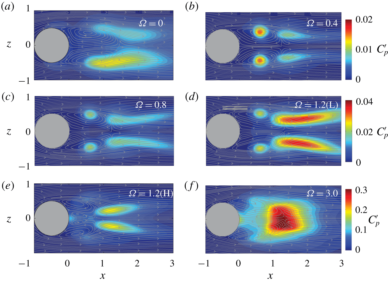
 $c_{x}$, and complex trajectories in the phase diagrams of figure 10(a–c). The differences in topology between regimes are further illustrated in figure 11 by means of contours of standard fluctuations of the pressure coefficient,
 $C_{p}^{\prime }$, and time-averaged velocity streamlines at
 $y=0$. The irregular vortex-shedding regime at
 $\unicode[STIX]{x1D6FA}=0$ displays a higher level of fluctuations along the shear layers, whereas for the periodic and quasi-periodic regimes for
 $\unicode[STIX]{x1D6FA}\leqslant 1.3$ (i.e. low-drag behaviour), the largest magnitude of
 $C_{p}^{\prime }$ is distributed at the cores of recirculating bubble and downstream of it. In general, the magnitude of the pressure fluctuations increases with
 $\unicode[STIX]{x1D6FA}$, while the recirculating cores move towards outer radial locations. The picture differs for the high-drag regime (see
 $\unicode[STIX]{x1D6FA}=1.2$ H in figure 11), whose wake is characterized by a double-celled recirculating bubble.
Contours of fluctuations of the pressure coefficient,  $C_{p}^{\prime }$, along with time-averaged velocity streamlines at
 $y=0$ for selected values of the rotation parameter
 $\unicode[STIX]{x1D6FA}$ at
 $Re=500$.

Note that similar double-celled structures were identified by Ruith et al. (Reference Ruith, Chen, Meiburg and Maxworthy2003) for swirling flows with wake-like axial velocity profiles at intermediate values of the rotation rate and Reynolds number. Moreover, the near wake displays intense fluctuations downstream of the recirculating bubble, which is now abruptly shortened.
Finally, the irregular shedding regime observed at large values of the rotation rates (see, e.g.  $\unicode[STIX]{x1D6FA}=3$) displays again a single vortex ring in the near wake. A wide region of high magnitude of
 $C_{p}^{\prime }$ is found at the axis and rear end of the recirculating bubble, where the fluctuations are more intense.
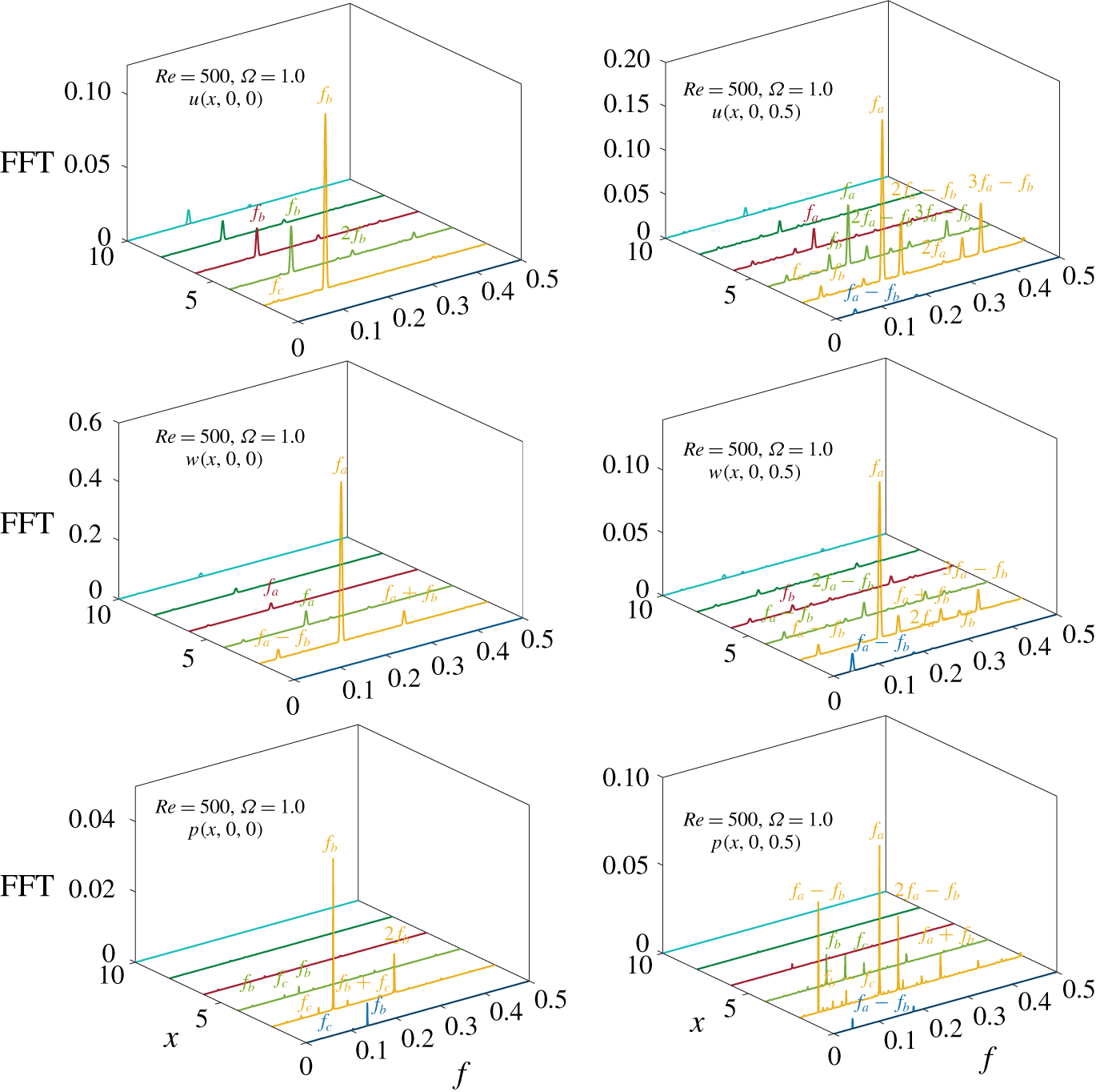
4.2 Frequency analysis
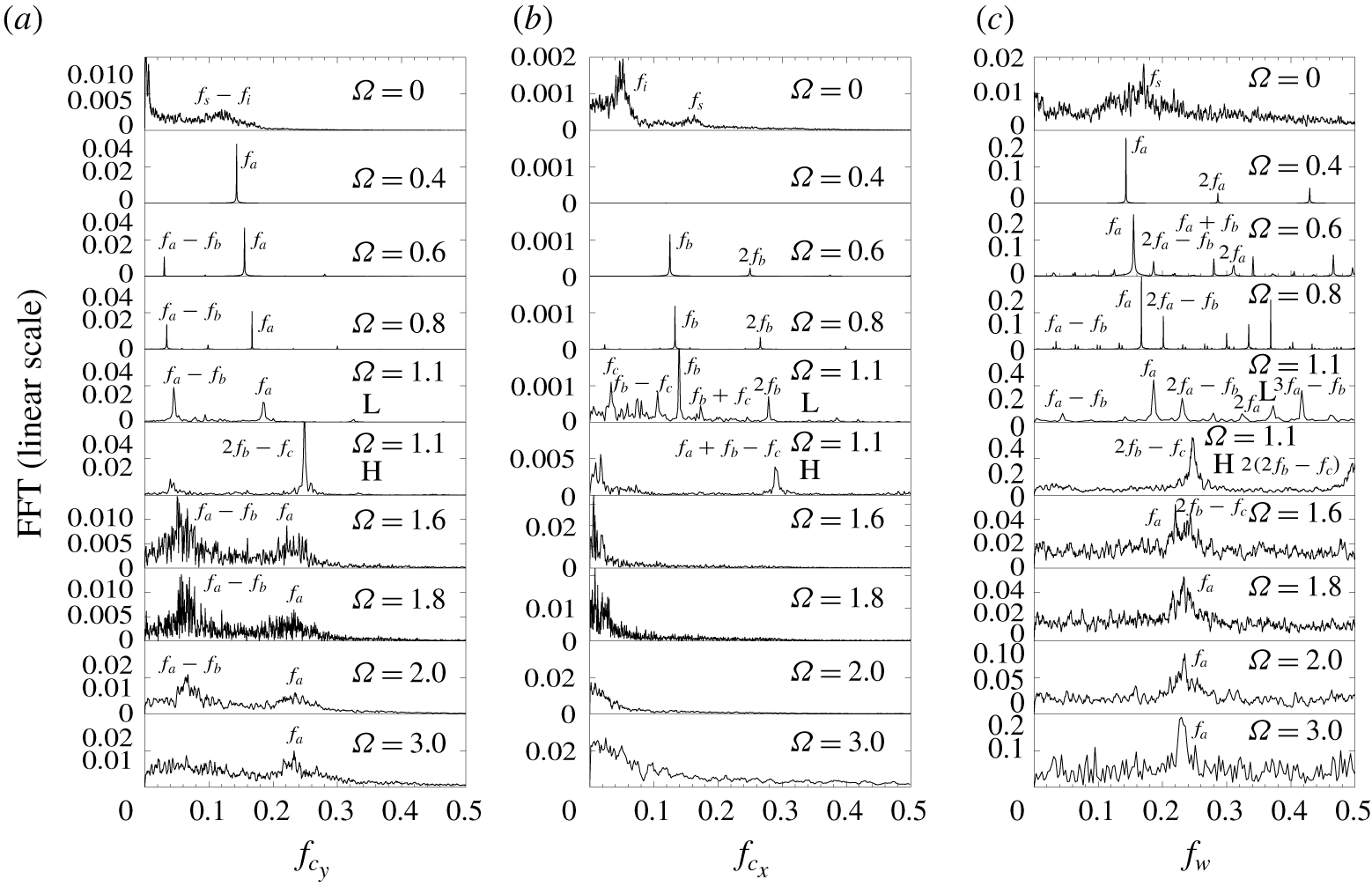
In figure 12 we show the FFT spectra of fluctuating values of forces  $c_{y}^{\prime }(t)$ and
 $c_{x}^{\prime }(t)$, and the azimuthal velocity
 $w^{\prime }(t)$ taken at
 $(x,y,z)=(2,0.5,0)$ for selected values of the rotation rate
 $\unicode[STIX]{x1D6FA}$. To follow the same approach as in § 3, fundamental dominant frequencies will be identified according to their different nature, so that
 $f_{a}$ is related to wake threads rotation,
 $f_{b}$ to shedding or
 $f_{c}$ for secondary helical dynamics.
Fast Fourier transform spectra, listing main frequency components, for different rotation parameters,  $\unicode[STIX]{x1D6FA}$, at
 $Re=500$, corresponding to the (a)
 $y$-axis lift coefficient,
 $c_{y}^{\prime }=c_{y}-C_{y}$, (b) drag coefficient,
 $c_{x}^{\prime }=c_{x}-C_{x}$, and the (c) azimuthal velocity
 $w^{\prime }=w-W$ at
 $(x,y,z)=(2,0.5,0)$. The computation of FFT spectra at
 $\unicode[STIX]{x1D6FA}=1.1$ for low- and high-drag regimes have been performed using conditional time series.

First, the spectra associated to the irregular regime at  $\unicode[STIX]{x1D6FA}=0$ display broad frequency components, with two main peaks at
 $f_{s}=0.163$ and
 $f_{i}=0.049$, which are respectively associated to the vortex shedding (
 $f_{s}$) and the irregular azimuthal pulsation of the shedding point at the sphere’s rear (
 $f_{i}$). In particular, the peaks of the shedding process are neater for
 $c_{x}^{\prime }$ and
 $w^{\prime }$, while the lift
 $c_{y}^{\prime }$ seems to be dominated by the combination of previous main frequencies
 $f_{s}-f_{i}$.
As the rotation is applied, the wake organizes itself, and as observed in the FFT spectra of  $c_{y}^{\prime }$ and
 $w^{\prime }$, the dynamics is mainly dominated by the single frequency,
 $f_{a}=f_{s}-f_{i}$, which corresponds to the rate of rotation of the vortical structures depicted in figure 9 (harmonics
 $2f_{a}$ and
 $3f_{a}$ are also identified in the FFT spectra of
 $w^{\prime }$). Thus, such a regime emerges after a wake synchronization at the combination of former shedding process frequencies,
 $f_{s}-f_{i}$. The frozen behaviour renders the flow steady from a reference system rotating with the wake and, consequently, the FFT spectra f
 $c_{x}^{\prime }$ does not display any significant peak in figure 12. Note that, unlike the frozen state reported at
 $Re=250$, now the rate is
 $f_{a}/f_{r}>1$, indicating that the wake rotates faster than the sphere.
A slight increase of the rotation rate up to 0.6 leads to the emergence of a new incommensurate frequency peak  $f_{b}$ in the FFT spectra of drag
 $c_{x}^{\prime }$, which may be related to the vortex shedding from the internal near wake spiral identified earlier. Additionally, a secondary peak emerges in the FFT spectra of
 $c_{y}^{\prime }$, that is, the nonlinear combination of both wake rotation and shedding frequencies, i.e.
 $f_{a}-f_{b}$, thus leading to the quasi-periodic time series
 $c_{y}(t)$ and phase portraits
 $(c_{y},c_{z})$ of figure 10. Moreover, the wake also displays harmonic and derived frequencies downstream (see the FFT spectra of
 $w^{\prime }$).
The energy content of such frequencies rises as the rotation increases up to  $\unicode[STIX]{x1D6FA}=1.1$ for the L regime, where the spectra display broader features, indicating more complex wake dynamics, although the same coherent peaks are still mostly recognizable. However, a new incommensurate frequency
 $f_{c}$ is observed in the FFT spectra of drag
 $c_{x}^{\prime }$. This tertiary low-frequency component may represent a modulation of the shedding process governed by
 $f_{b}$, considering the existence of nonlinear interactions
 $f_{b}-f_{c}$ and
 $f_{b}+f_{c}$ in the spectrum. Then, such low-frequency pulsation seems to be the precursor for the sudden topological change observed in the near wake of the H regime, whereby the two-celled recirculating bubble appears (figure 11). In particular, the different dynamics obtained at
 $\unicode[STIX]{x1D6FA}=1.1$ for the H regime is mainly governed by the combined frequency
 $f=2f_{b}-f_{c}$ and its harmonic
 $2f=2(2f_{b}-f_{c})$, in view of the FFT spectra of
 $w^{\prime }$ (figure 12), being the latter frequency associated to the existence of energetic
 $m=2$ structures at the wake (figure 9), as will be shown below. Other combinations of previously reported frequencies are visible in the FFT spectra of
 $c_{y}^{\prime }$ and
 $c_{x}^{\prime }$, e.g. the nonlinear components
 $f_{a}-f_{b}$ and
 $(2f_{b}-f_{c})+(f_{a}-f_{b})=f_{a}+f_{b}-f_{c}$. The peaks display generally broader bases, indicating more irregular dynamics than that of the L regime (as in the phase diagrams in figure 10b,c). Thus, the reported H regime seems to arise as a process of wake synchronization at a derived frequency from the two incommensurate values
 $f_{b}$ and
 $f_{c}$. As generally occurs in bistable flows (see e.g. Cadot, Evrard & Pastur Reference Cadot, Evrard and Pastur2015), the random switching between both wake states might be triggered by any flow perturbation that selects predominantly one of the states.
Finally, for  $\unicode[STIX]{x1D6FA}>1.4$, the wake becomes more irregular, being the dominant frequencies
 $f_{a}$ and the interaction
 $f_{a}-f_{b}$, indicating that the wake dynamics is mainly governed by the low-drag regime frequency features. For such rotation rates, all the displayed FFT spectra are characterized by noisy, broadband peaks, indicating a potential transition to chaos. As in § 3, to analyse the spatial prevalence of the frequencies, we display in figure 13 the FFT spectra of axial and transverse velocities,
 $u$ and
 $w^{\prime }$, and pressure,
 $p^{\prime }$, at
 $x\leqslant 10$ and
 $r=[0,0.5]$ for
 $\unicode[STIX]{x1D6FA}=1$, where the three incommensurate frequencies
 $f_{a}$,
 $f_{b}$ and
 $f_{c}$ are present. In general, the largest spectral magnitudes are found at
 $x=2$. In addition, it can be observed that the frequency
 $f_{a}$ displays energetic peaks in the FFT spectra computed at
 $r=0.5$ for all variables and prevails at least until
 $x=10$. The fundamental frequency component
 $f_{b}$ is particularly energetic in
 $r=0$ for the axial velocity
 $u^{\prime }$ and pressure
 $p^{\prime }$, which suggests that the associated phenomenon takes place at a centred location, as the shedding process from the inner spiral shown in figure 9. Additionally, the low-frequency peak
 $f_{c}$ arises in the spectra of the axial velocity,
 $u^{\prime }$, and pressure,
 $p^{\prime }$, at
 $r=0$ and the near wake for
 $x<4$, so that it might be related to a pulsation of the recirculating bubble, that triggers the sudden transition to the H regime at
 $\unicode[STIX]{x1D6FA}=1.1$, through the activation of the reported frequency component
 $2f_{b}-f_{c}$. Finally, the combined frequency
 $f_{a}-f_{b}$ stands out as an especially intense peak in the FFT spectrum of
 $p^{\prime }$ at
 $r=0.5$, and observable for
 $w^{\prime }$ at both radial locations, but limited to
 $x\leqslant 6$, which is compatible with a near wake helical structure, as will be shown below.
Fast Fourier transform spectra of the axial and transverse velocities,  $u^{\prime }=u-U$ and
 $w^{\prime }=w-W$, and pressure,
 $p^{\prime }=p-P$, at downstream axial locations,
 $(x\leqslant 10)$, and radial locations
 $r=[0,0.5]$ for the selected value of
 $\unicode[STIX]{x1D6FA}=1$ and
 $Re=500$.

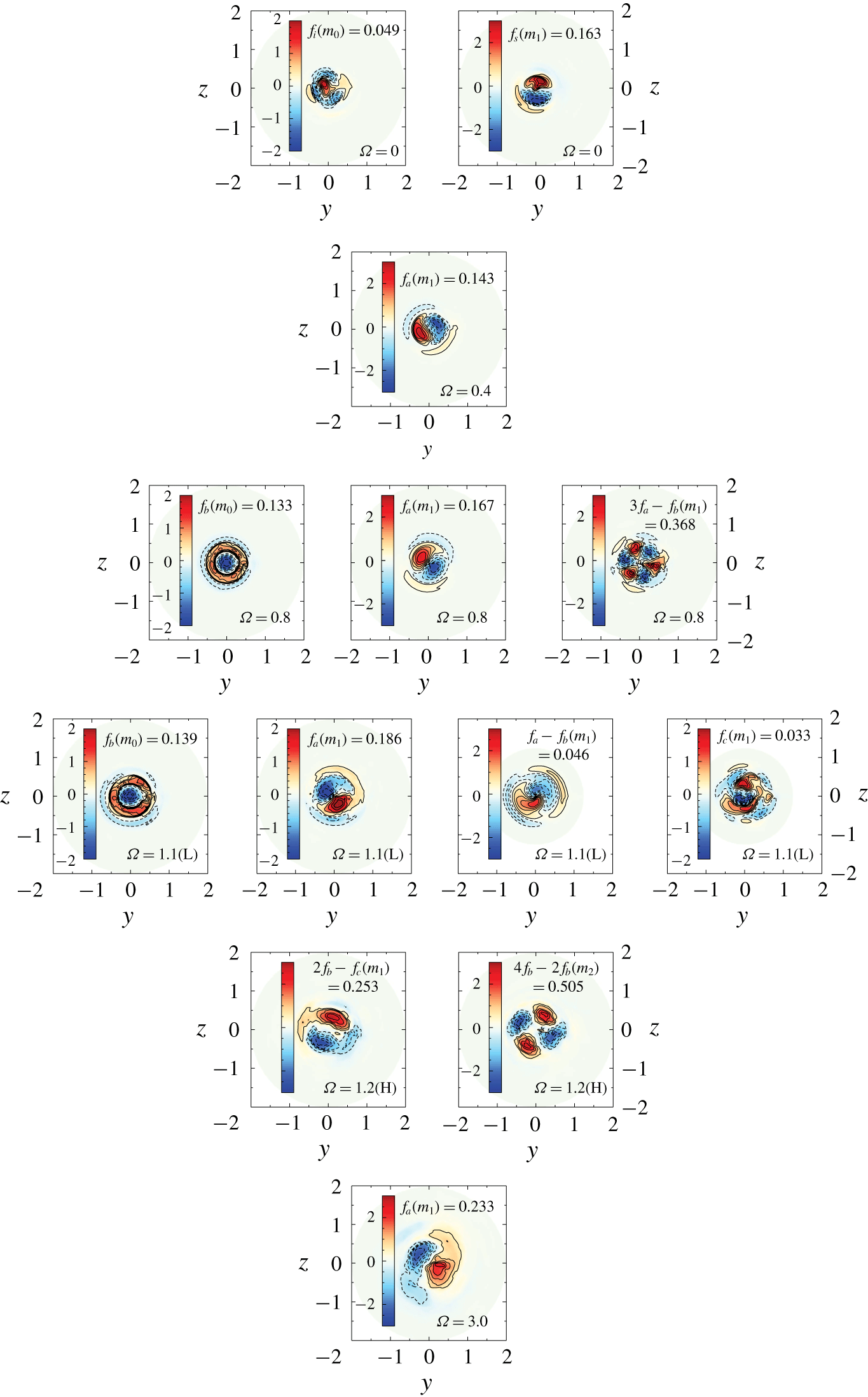
Contours of the axial vorticity  $\unicode[STIX]{x1D71B}_{x}$ (real part), for the most energetic modes identified through HODMD analysis at
 $x=2$, for selected values of
 $\unicode[STIX]{x1D6FA}$ at
 $Re=500$. Modes are arranged from left to right in increasing order of azimuthal wavenumber.

4.3 Flow decomposition
4.3.1 Higher-order dynamic mode decomposition
To conclude the discussion on the flow regimes for  $Re=500$, we apply again the HODMD analysis at
 $x=2$. Results are summarized in figure 14, where contours of the normalized axial vorticity
 $\unicode[STIX]{x1D71B}_{x}$, corresponding to dominant modes with the largest growth rate, are displayed for selected values of the rotation rate
 $\unicode[STIX]{x1D6FA}$. Without rotation (
 $\unicode[STIX]{x1D6FA}=0$), the wake is dominated by two fundamental frequencies,
 $f(m_{1})=0.163$ and
 $f(m_{0})=0.049$, which respectively correspond to the shedding frequency,
 $f_{s}$, and the irregular azimuthal rotation rate of the shedding location,
 $f_{i}$, identified in the spectrum of
 $c_{x}^{\prime }$ in figure 12. The vortex shedding mode presents an azimuthal symmetry
 $m_{1}$, with two counter-rotating vortices, while the irregular rotation of the shedding location explores approximately the whole azimuth at the rear of the sphere, so that the mode can be considered statistically axisymmetric (note that the slow dynamics of such phenomenon would require a very long time history of snapshots to fully retrieve the statistical axisymmetry).
For  $\unicode[STIX]{x1D6FA}=0.4$, the wake was shown to display periodic dynamics that is retrieved at the flow decomposition, which only identifies an unstable mode with frequency
 $f_{m_{1}}=0.143\equiv f_{a}$, related to a dipole of axial vorticity close to the axis and an induced vorticity around them. Such periodic dynamics is broken as
 $\unicode[STIX]{x1D6FA}$ grows, as seen, for instance, when
 $\unicode[STIX]{x1D6FA}=0.8$, due to the occurrence of a nearly axisymemtric shedding of frequency
 $f_{m_{0}}=0.133\equiv f_{b}$. This mode presents a negative vorticity of high intensity at the axis, coinciding with the location of the near wake spiral (see figure 9), from where vortices are detached. Additionally, HODMD identifies secondary frequency components in the form
 $f=n_{1}f_{a}\pm n_{2}f_{b}$, with
 $n_{1}$ and
 $n_{2}$ being natural numbers. As an instance, the energetic mode with
 $f=0.368$, which correspond to
 $3f_{a}-f_{b}$ in figure 12 is displayed. As expected from the simple interaction of frequencies, the structures show an
 $m_{3}$ symmetry.
The scenario changes at  $\unicode[STIX]{x1D6FA}=1.1$, where the quasi-periodic dynamic is strongly modulated by the new frequency component
 $f_{c}$, which is mainly identified in the FFT spectra of
 $c_{x}^{\prime }$ and
 $p^{\prime }$ in the near wake. According to the decomposition, a new mode of frequency
 $f=0.033\equiv f_{c}$ and moderate amplitude is present at the flow, and is characterized by a helical structure featuring an entangled spiral dipole of vorticity. Thus, it constitutes a wake modulation phenomenon with an
 $m_{1}$ symmetry. In addition, the complexity of the wake at the L regime is also the outcome of the strengthening of derived frequencies, as the
 $f_{a}-f_{b}=0.046$, whose helical structure presents an
 $m_{1}$ symmetry as expected from the interaction between previously described modes
 $f_{a}$ and
 $f_{b}$.
The analysis of the wake corresponding to the high-drag regime clearly identifies the energetic frequency components  $f=0.253$ and its harmonic
 $2f=0.505$, which correspond to the peaks of
 $2f_{b}-f_{c}$ and
 $2(2f_{b}-f_{c})$ previously observed in the FFT analysis. The interaction between fundamental frequencies entails that both modes present respectively helical
 $m_{1}$ and
 $m_{2}$ azimuthal symmetries. The elongated contours featured by the component
 $2f_{b}-f_{c}$ anticipates the existence of the intense spiral topology and incipient vortex loops. Interestingly, the modes do not present vorticity close to the axis, which can be associated to the existence of the double-celled recirculating region in the near wake.
Finally, the irregular regime established for  $\unicode[STIX]{x1D6FA}>1.4$ is fundamentally characterized by
 $m_{1}$ structures associated to the frequency component
 $f_{a}$, that now presents a larger radial extension than in the precedent regime. In particular, unlike the previous modes governing the wake dynamics for the H regime, the structures cover the vicinity of the axis and are more elongated, indicating a tilting of threads that leads to the connection and formation of vortex loop, as displayed in figure 9.
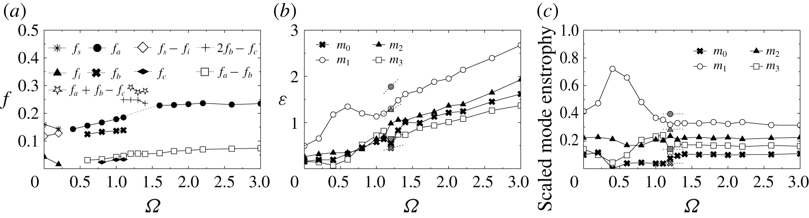
Flow decomposition at  $Re=500$: evolution with
 $\unicode[STIX]{x1D6FA}$ of the (a) characteristic frequencies corresponding to dominant modes; (b) enstrophy,
 $\unicode[STIX]{x1D700}(m)$, for the most energetic azimuthal symmetries (FAD); and the (c) relative contribution to the total enstrophy for symmetries
 $m=0,1,2$ and 3 (FAD). The vertical lines in (b,c) distinguish regimes with different dominant azimuthal symmetries. Black and white filled symbols in (a) respectively represent fundamental and combined frequencies; while grey symbols in (b,c) stand for values obtained at the conditional high-drag regime.

A summary of the evolution of the dominant frequencies, associated to the most energetic modes at the wake, is included in figure 15(a). As observed, the irregular shedding regime at low  $\unicode[STIX]{x1D6FA}$ is governed by both the shedding frequency,
 $f_{s}$, and the azimuthal rotation of the shedding point related to
 $f_{i}$. The combined frequency
 $f_{s}-f_{i}$ grows linearly with
 $\unicode[STIX]{x1D6FA}$ and becomes dominant at
 $\unicode[STIX]{x1D6FA}=0.4$, where the wake becomes frozen and rotates periodically at the synchronization frequency
 $f_{a}=f_{s}-f_{i}$. The shedding frequency
 $f_{b}$ appears at
 $\unicode[STIX]{x1D6FA}=0.6$, rendering the wake dynamics quasi-periodic. Both
 $f_{b}$ and the nonlinear combination
 $f_{a}-f_{b}$ grow monotonously with
 $\unicode[STIX]{x1D6FA}$ up to 1.1 approximately. The destabilization of the frequency
 $f_{c}$ around
 $\unicode[STIX]{x1D6FA}=1$ implies that the modulation of quasi-periodic dynamics reported for the low-drag regime, within the range
 $1.1\leqslant \unicode[STIX]{x1D6FA}\leqslant 1.3$, while its quadratic interaction with
 $f_{b}$, i.e.
 $2f_{b}-f_{c}$, governs the dynamics of the high-drag regime together with the secondary frequencies
 $2(2f_{b}-f_{c})$ (of
 $m_{2}$ symmetry) and
 $f_{a}+f_{b}-f_{c}$. Finally, the irregular wake observed for
 $1.4\leqslant \unicode[STIX]{x1D6FA}\leqslant 3$ is characterized by frequencies
 $f_{a}$ and
 $f_{a}-f_{b}$, which display nearly constant values as the rotation parameter increases.
4.3.2 Fourier azimuthal decomposition
The competition between azimuthal symmetries is further evaluated by means of the FAD analysis at  $x=2$. The evolution of the enstrophy for the first four azimuthal wavenumbers,
 $\unicode[STIX]{x1D700}(m)$, is plotted in figure 15(b). As observed, the symmetry
 $m=1$ (
 $m_{1}$) is the dominant one for the whole range of
 $\unicode[STIX]{x1D6FA}$ investigated. In particular, it grows considerably during the irregular shedding and frozen regime for
 $\unicode[STIX]{x1D6FA}\leqslant 0.6$, where the spiral structures dominate the flow, decreasing slightly as the quasi-periodic regime sets in the wake, since the shedding from the inner spiral associated to
 $f_{b}$ (
 $m_{0}$) and the harmonics, especially
 $3f_{a}-f_{b}$ (
 $m_{3}$),
 $2f_{a}-f_{b}$ and
 $f_{a}$ (
 $m_{2}$) develop at the flow. Thus, the enstrophy associated to these azimuthal symmetries start to grow almost linearly until
 $\unicode[STIX]{x1D6FA}=1.1$. The emergence of
 $f_{c}$ around
 $\unicode[STIX]{x1D6FA}=1$, compensate the decrease of
 $\unicode[STIX]{x1D700}(m_{1})$, which starts to grow again with
 $\unicode[STIX]{x1D6FA}$. The H regime, represented in the figure using grey symbols for conditionally averaged values, features an important growth in the enstrophy of
 $m_{1}$ and
 $m_{2}$ due the presence of energetic structures associated to the derived frequency
 $2f_{b}-f_{c}$ and its harmonic
 $2(2f_{b}-f_{c})$. For
 $\unicode[STIX]{x1D6FA}\geqslant 1.4$, all the modes display linear increases of
 $\unicode[STIX]{x1D700}$. However, the
 $m_{2}$ symmetry displays a larger energy content than
 $m_{0}$ and
 $m_{3}$, which may be associated to the weakening of the mode associated to
 $f_{b}$, and its derived component
 $3f_{a}-f_{b}$.
An alternative FAD analysis is performed to the fluctuating values of vorticity  $\unicode[STIX]{x1D71B}_{x}^{\prime }(t)=\unicode[STIX]{x1D71B}_{x}-\unicode[STIX]{x1D6F1}_{x}$, to eliminate the effect of cyclonic vorticity. The scaled contribution of each mode is displayed in figure 15(c) as a function of
 $\unicode[STIX]{x1D6FA}$. As observed,
 $m_{1}$ structures dominate the wake dynamics at low values of
 $\unicode[STIX]{x1D6FA}$. Initially, some energy content exists for the remaining modes,
 $m=0,~2$ and 3, due to the irregular nature of the shedding regime with multiple frequency components. However, the occurrence of the periodic regime around
 $\unicode[STIX]{x1D6FA}=0.4$ implies a wake arrangement that fosters the
 $m_{1}$ rotating structures (which represents approximately 75
 $\,\%$ of the total enstrophy), whereas the remaining symmetries are weakened. Within the interval
 $0.6\leqslant \unicode[STIX]{x1D6FA}\leqslant 1.1$, the quasi-periodic regime enhances the symmetries
 $m=0,2$ and 3 due to the emergence of the axisymmetric shedding in the inner thread related to
 $f_{b}$, and the development of harmonics and derived frequencies.
During the H regime,  $m_{1}$ and
 $m_{2}$ account for 70
 $\,\%$ of the total enstrophy, reducing the relative contribution of
 $m_{0}$ and
 $m_{3}$. Finally, for
 $\unicode[STIX]{x1D6FA}\geqslant 1.4$, the wake complexity of the irregular regime is related to the excitation of different azimuthal modes (the enstrophy
 $\unicode[STIX]{x1D700}(m_{1})$ barely reaches 30
 $\,\%$ of the total one), leading to a weaker wake coherence and the existence of multiple scales, as observed in figure 9.
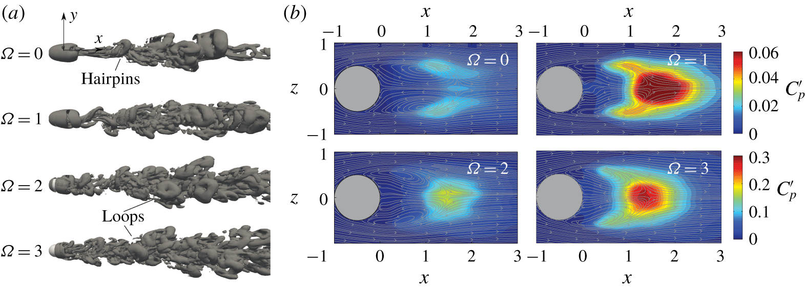
5 Flow regimes behind a streamwise rotating sphere at Re $=$ 1000

(a) Isosurfaces of the  $Q$-quantity (
 $Q=10^{-2}$) at
 $Re=1000$ and selected values of the rotation parameter
 $\unicode[STIX]{x1D6FA}$. Note that the lateral view extends a downstream distance of
 $x=20D$ from the sphere’s rear end. (b) Corresponding contours of fluctuations of the pressure coefficient,
 $C_{p}^{\prime }$, along with time-averaged velocity streamlines at
 $y=0$.

5.1 Qualitative description of flow regimes
The analysis of the transitional wake behind a streamwise rotating sphere is finished with the study of flow regimes at  $Re=1000$, which are summarized in figure 16, that displays, for selected values of
 $\unicode[STIX]{x1D6FA}$, instantaneous plots of vortical structures by means of isocountours of the
 $Q$-quantity (figure 16a) and time-averaged contours of standard fluctuations of the pressure,
 $C_{p}^{\prime }$, in the near wake. As in Tomboulides & Orszag (Reference Tomboulides and Orszag2000), an irregular vortex-shedding regime is obtained for
 $\unicode[STIX]{x1D6FA}=0$, where the dominant frequency is
 $f_{s}=0.188$. As displayed in figure 16(a), small scales are clearly present at the flow, rendering it turbulent, although large-scale hairpin vortices are evident. As in
 $Re=500$, there is an azimuthal rotation of the shedding location and, therefore, the hairpin vortices display different orientations as are convected downstream. The shedding intensifies the pressure fluctuations (figure 16b) along the shear layers, as in the irregular regime of
 $Re=500$.
With rotation, the wake displays similar irregular dynamics, characterized by the rapid rotation and massive separation of vortex loops, of a smaller length scale, which are now distributed along different azimuthal positions. At high values of  $\unicode[STIX]{x1D6FA}$, the formation of hairpin vortices seems to take place directly at the shear layer of the sphere. Such modified dynamics strengthen the pressure fluctuations at the rear of the recirculation bubble, as occurs for
 $Re=500$ and
 $\unicode[STIX]{x1D6FA}\geqslant 1.4$, suggesting that the wake regimes are similar.
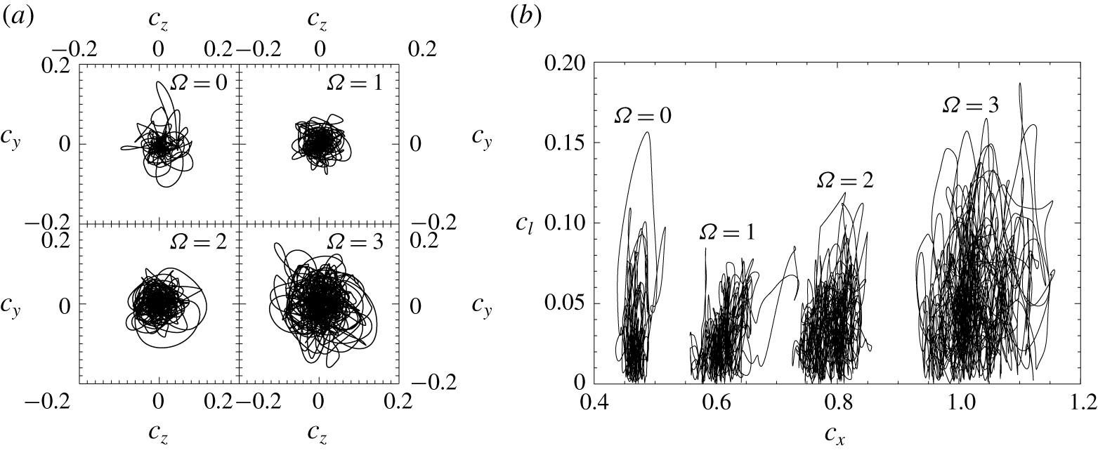
The complexity of the wake dynamics is observable in the phase diagrams of the force coefficients  $(c_{y},c_{z})$ and
 $(c_{x},c_{l})$ of figure 17. The irregular state produces entangled phase portraits, with an increasing magnitude of fluctuations as
 $\unicode[STIX]{x1D6FA}$ grows. In particular, due to the fostering of the shedding process, the fluctuations of the drag coefficient increase, as shown by the wider diagrams at large
 $\unicode[STIX]{x1D6FA}$. In addition, a larger radial extension of
 $(c_{y},c_{z})$ diagrams, which explore statistically the whole azimuth, is seen with the increase of
 $\unicode[STIX]{x1D6FA}$, indicating an intense wake rotation and a higher eccentricity, that enhances the magnitude of the fluctuating lift coefficient in the
 $(c_{x},c_{y})$ plot. These portraits are similar to those corresponding to the irregular regime at
 $Re=500$ and
 $\unicode[STIX]{x1D6FA}\geqslant 1.4$.
5.2 Frequency analysis
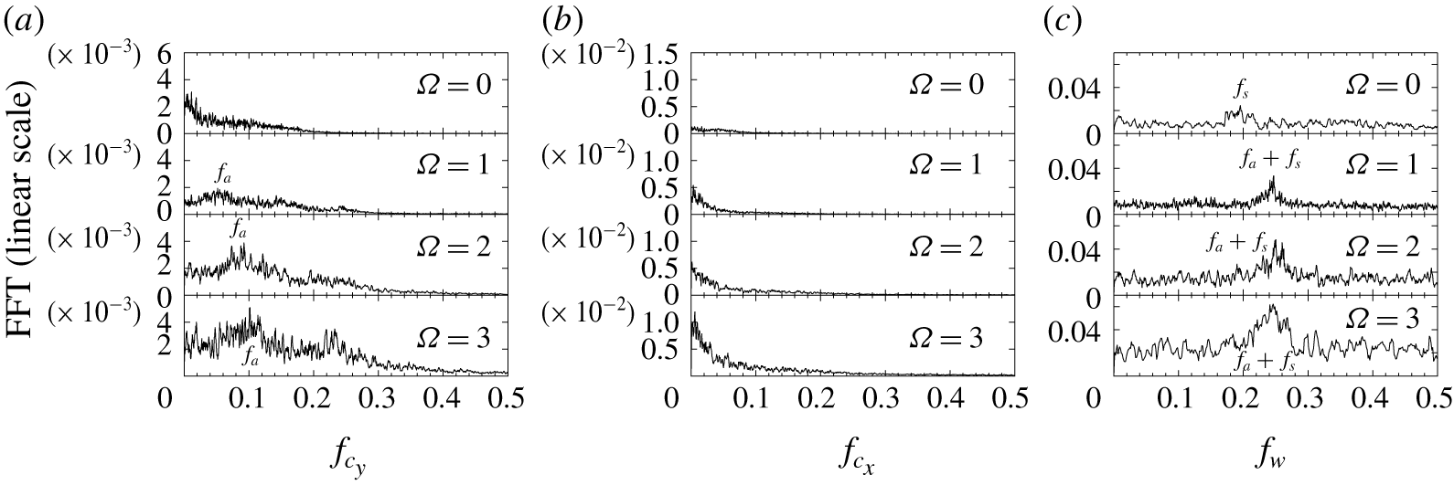
As in the previous sections, we analyse the dominant frequency components from the FFT of fluctuating forces  $c_{y}^{\prime }(t)$ and
 $c_{x}^{\prime }(t)$, and the azimuthal velocity
 $w^{\prime }(t)$ at the location
 $(x,y,z)=(2,0.5,0)$, which are represented in figure 18 for selected values of
 $\unicode[STIX]{x1D6FA}$. As observed, at
 $\unicode[STIX]{x1D6FA}=0$, the spectra display broad features and it is difficult to infer dominant frequencies from the force coefficients spectra. In both cases, a large energy content exists close to
 $f=0$, however, in the case of the azimuthal velocity (figure 18c) the shedding frequency can be identified as
 $f_{s}=0.188$, which, as expected, is slightly higher than that reported for
 $Re=500$. With the streamwise rotation, the wake displays similar dynamics for the whole interval of
 $\unicode[STIX]{x1D6FA}$ investigated. In particular, a new frequency
 $f_{a}$ is discernible at the spectra of
 $c_{y}^{\prime }$ for
 $\unicode[STIX]{x1D6FA}\geqslant 0.4$, which is related to the wake rotation, while the corresponding peak associated to the shedding is now modified, corresponding it to
 $f_{s}+f_{a}$ as observed in the FFT spectra of
 $w^{\prime }$. In general, the dynamics is characterized by the slow rotation of vortical structures with a frequency
 $f_{a}$, and the massive shedding of vortex loops, whose frequency
 $f_{a}+f_{s}$ accelerates with rotation until reaching a nearly constant value at higher
 $\unicode[STIX]{x1D6FA}$. The spectra are characterized by broader features and multiple frequencies, as expected for the complex and irregular flow behaviour reported earlier. Such seemingly chaotic dynamics render it difficult to identify clear frequency components, along with coherent structures of the dominant modes at the wake, which precluded us from performing such analysis. The complexity and possible chaotic nature of the flow dynamics will be further analysed in § 7.
Force coefficients at  $Re=1000$: (a) phase diagrams of transversal forces (
 $c_{z},c_{y}$); and (b) phase diagrams of the total lift versus drag (
 $c_{l},c_{x}$).

Fast Fourier transform spectra, listing the main frequency components, for different rotation parameters,  $\unicode[STIX]{x1D6FA}$, at
 $Re=1000$, corresponding to the (a)
 $y$-axis lift coefficient,
 $c_{y}$, (b) drag coefficient,
 $c_{x}$, and the (c) azimuthal velocity
 $w$ at
 $(x,y,z)=(2,0.5,0)$.

6 Time-averaged force coefficients and recirculation length
Evolution of time-averaged force coefficients with  $\unicode[STIX]{x1D6FA}$: (a) drag coefficient,
 $C_{x}$ (solid line), (b) total lateral force coefficient,
 $C_{l}$ and (c) time-averaged recirculation length,
 $L_{r}$. The grey symbols represent values obtained for the high-drag regime.

Next we present in figure 19 the evolution with the rotation rate  $\unicode[STIX]{x1D6FA}$ of time-averaged force coefficients. In particular, mean values of the drag coefficient
 $C_{x}$ (figure 19a) and the total lift
 $C_{l}$ (figure 19b) are included for discussion. First, it is seen that without rotation, the drag decreases as the Reynolds number rises due to the progressively less relevant viscous contribution (figure 19a). That said, the mean drag is seen to increase quadratically with
 $\unicode[STIX]{x1D6FA}$ for all values of
 $Re$.
Interestingly, the change of regimes is not observable in trends of  $C_{x}(\unicode[STIX]{x1D6FA})$, which increases monotonically, unlike the values of the mean recirculating region length,
 $L_{r}$, displayed in figure 19(c). Thus, the reason for the progressive increment in drag is a global decrease of the base pressure inversely related to the increase of the azimuthal velocity, while the pressure is mostly unchanged at the front.
To illustrate this, in figure 20(a) we plot contours of the averaged pressure distributions and streamlines at the plane  $y=0$ for different values of
 $\unicode[STIX]{x1D6FA}$ and
 $Re=500$. Without rotation, the wake displays an elongated recirculation bubble, which is associated to low values of the mean pressure coefficient. As
 $\unicode[STIX]{x1D6FA}$ increases, the changes in the recirculation bubble are smooth but sensitive to the wake regime, however, the pressure decrease is progressive, until reaching very low values for
 $\unicode[STIX]{x1D6FA}=3$ (an exception of such monotonous decrease being the emergence of the H regime around
 $\unicode[STIX]{x1D6FA}=1.1$, for which the pressure decay is intensified on account of the strong topological changes of the flow).
(a) Time-averaged pressure distribution,  $C_{p}$, and streamlines at
 $y=0$ for selected values of the rotation rate
 $\unicode[STIX]{x1D6FA}$ and
 $Re=500$. (b) Radial profiles of the time-averaged axial velocity,
 $U$, taken at
 $x=0.5$ and
 $y=0$ for selected values of
 $\unicode[STIX]{x1D6FA}$.

In view of figure 20(a), two mechanisms can be associated to such changes in the pressure coefficient. First, the recirculation bubble shortening observed for some regimes approaches the recirculation eddies to the sphere. Second, a general shift of such loci of recirculation towards outer radial locations, caused by the centrifugal force induced by the increasing rotation rate, is also observed. An important swelling of the recirculation region exists, changing the curvature of the separatrix, since the boundary layer detachment moves upstream as  $\unicode[STIX]{x1D6FA}$ rises, due to the higher adverse pressure gradient induced by the centrifugal effect (as discussed by Wu (Reference Wu1972) for inviscid flows, at first order, the low base pressure is produced by the flow curvature around the body, since the centripetal acceleration produced by the streamlines curvature surrounding the separated region is balanced by a pressure gradient in the Euler equations; which also holds for viscous wake flows, as shown by Roshko (Reference Roshko1993)). Thus, the higher curvature of the separatrix would lead to the reported pressure decrease as
 $\unicode[STIX]{x1D6FA}$ grows. As shown in figure 20(b), where the radial profiles of the mean axial velocity
 $U(x=0.5,r)$ are depicted, stronger axial velocity backflow and velocity deficit are generally observed for increasing values of
 $\unicode[STIX]{x1D6FA}$.
Regarding the H regime, the recirculation region is shown to be considerably shortened (see grey symbols in figure 19c), and an internal recirculation region is induced by the destabilization of the modulating dynamics of the near wake, as discussed in § 4. Such a topology change entails an abrupt decrease of pressure (figure 20a) and, consequently, a higher drag coefficient, as depicted in figure 19(a), although the magnitude of the associated velocity backflow is clearly lower than that of the L state (see profiles of  $\unicode[STIX]{x1D6FA}=0.8$ and 1.2 in figure 20b).
In addition, the mean value of the total lift,  $C_{l}$, is depicted in figure 19(b), where it can be observed that trends are not monotonous and change with the flow regimes, as
 $L_{r}$ does (figure 19c). For low values of
 $\unicode[STIX]{x1D6FA}$,
 $Re=250$ is shown to display a larger mean lift, which stems from the original eccentricity induced by the SS state. In general,
 $C_{l}$ first decreases when the flow evolves towards a frozen regime, and starts to increase with
 $\unicode[STIX]{x1D6FA}$ within the quasi-periodic regimes, whereas abrupt transitions are shown when irregular regimes emerge for
 $Re=250$ and 500. Moreover, it is also seen that within the irregular regimes for
 $Re\geqslant 500$, the value of the mean lift rises monotonously with the growth of
 $\unicode[STIX]{x1D6FA}$, on account of the increasing eccentricity due to centrifugal effects. For
 $Re=1000$, there is an initial decrease of
 $C_{l}$ and an increase of
 $L_{r}$ with
 $\unicode[STIX]{x1D6FA}$, which are reverted with the development at the wake of the peak
 $f_{a}$ associated to the strong rotation of vortical structures.
7 Bifurcation diagrams and chaos test
To conclude the discussion on the flow regimes, we present the bifurcations diagrams for  $Re=250$ and 500 (which display richer transition patterns than
 $Re=1000$) in figure 21(a,c), obtained for increasing values of
 $\unicode[STIX]{x1D6FA}$. These bifurcation diagrams plot local maxima and minima of the time histories of the
 $y$-direction lift coefficient,
 $c_{y}$, depicted in figures 3 and 10, where the rotation rate
 $\unicode[STIX]{x1D6FA}$ plays the role of the free control parameter. In such diagram, a fixed point regime is represented by a single point, a stable limit cycle is identified by means of two symmetric points, while quasi-periodic and irregular or chaotic regimes feature multiple points. Additionally, the corresponding three-dimensional phase diagrams of velocity components obtained at
 $(x,y,z)=(2,0,0)$ for
 $Re=250$ and 500, are respectively depicted in figure 21(b,d) to illustrate the analysis.
(a,c) Bifurcation diagrams obtained by plotting maxima and minima of time histories of  $c_{y}$ against
 $\unicode[STIX]{x1D6FA}$ for
 $Re=250$ and 500. (b,d) Corresponding three-dimensional phase diagrams of velocity components obtained at
 $(x,y,z)=(2,0,0)$ (
 $u$-vertical axis,
 $v,w$-horizontal axes). The red dots in (c) represent the maxima and minima obtained for the high-drag regime (H), whose phase diagram is included in (d).

Starting with  $Re=250$, for
 $\unicode[STIX]{x1D6FA}=0$, the SS regime is characterized by a stable fixed-point attractor, which is destabilized through a Hopf bifurcation as the rotation is applied. Thus, the helical frozen regime presents two points in figure 21(a), and a closed orbit in the three-dimensional phase plot (figure 21b). At
 $\unicode[STIX]{x1D6FA}=0.6$ the dynamical system is attracted towards a quasi-periodic regime, which features a broader range of maxima and minima points of
 $c_{y}$, and is preserved up to
 $\unicode[STIX]{x1D6FA}=1.4$. As previously described, such a regime is characterized by two incommensurable frequencies and, therefore, describes a torus of dimension 2 (
 $T_{2}$) in the phase diagram of figure 21(b). For
 $\unicode[STIX]{x1D6FA}=1.6$, an abrupt change is observed at the bifurcation diagram, with wider ranges of local peaks in
 $c_{y}$, while the phase diagram now presents a complex pattern. The destabilization of such a high-helical irregular regime was shown to be related to the coexistence of three incommensurable frequency components, which might indicate that such a regime lies originally on a torus of dimension 3 (
 $T_{3}$). At
 $\unicode[STIX]{x1D6FA}=2.2$ the points in the bifurcation diagram are more bounded on account of the system synchronization, according to the phase diagram shown in figure 21(b). Finally, at
 $\unicode[STIX]{x1D6FA}\geqslant 2.4$, such a modulated quasi-periodic regime loses its stability and the system turns again into irregular, higher-order quasi-periodic states, identified by broader groups of points in the bifurcation diagram.
The scenario is more complex for  $Re=500$, as depicted in figure 21(c). Initially, the irregular regime at
 $\unicode[STIX]{x1D6FA}=0$ leads to synchronized, periodic dynamics at 0.4, corresponding to a stable limit cycle in figure 21(c,d). This limit cycle becomes unstable around
 $\unicode[STIX]{x1D6FA}=0.6$, leading to the quasi-periodic regime through the destabilization of a second, incommensurate frequency, describing a torus
 $T_{2}$ in the phase diagram. The maxima and minima in the bifurcation diagram become numerous as
 $\unicode[STIX]{x1D6FA}$ grows, indicating a higher-dimensional order. In particular, above
 $\unicode[STIX]{x1D6FA}=1$, a continuous line of maxima and minima points exist, coincident with the emergence of a third incommensurate frequency, indicating a transition towards a higher quasi-periodic, as represented in the irregular toroidal phase diagram. The bistable dynamics between
 $\unicode[STIX]{x1D6FA}=1.1$ and 1.3 is shown in figure 21(c) by means of additional red dots for the H regime. As observed, dense lines of points are also present, indicating high-order dynamics, although it must be noted that such regions are not connected as it occurs for the equivalent L regime (black points). Such a scenario is the outcome of irregular toroidal phase diagrams as the one displayed in figure 21(d). Finally, at higher values of
 $\unicode[STIX]{x1D6FA}$ the system again displays continuous representations of points, compatible with the complex nature of flow dynamics.
As mentioned earlier, the densification of maxima and minima points in the bifurcation diagrams may be an indication of a transition towards a chaotic state. Instead of computing the Lyapunov exponents (which is beyond the scope of the present work), the 0–1 test (Gottwald & Melbourne Reference Gottwald and Melbourne2004) is used here as a simple quantitative method to confirm the chaotic nature of regimes seen in the bifurcation diagrams, which can be applied directly to time series. More details are given in appendix B, and different validations of the method can be found in Gottwald & Melbourne (Reference Gottwald and Melbourne2009) for different dynamical systems. The method allows us to compute an estimate of the asymptotic growth rate  $K$ in such a way that 1 corresponds to chaotic behaviour while 0 is associated to regular dynamics. Results of the 0–1 test versus the rotation parameter
 $\unicode[STIX]{x1D6FA}$ are displayed in figure 22 for
 $Re=250$, 500 and 1000. As observed for
 $Re=250$, values of
 $K$ remain close to 0 for periodic regimes and low-order quasi-periodic regimes. At
 $\unicode[STIX]{x1D6FA}=1.6$ a transition is observed, with
 $K$ tending to 1 as the irregular regime sets in, which prevails up to
 $\unicode[STIX]{x1D6FA}=2.2$, where the high-helical quasi-periodic regime emerging from the wake synchronization produces a value of
 $K$ close to zero again. The progressive increase of the rotation parameter leads again to the departure from 0 to 1 of the
 $K$ values. A similar analysis is performed for
 $Re=500$, which displays chaotic dynamics (
 $K\simeq 1$) at
 $\unicode[STIX]{x1D6FA}<0.4$, within the irregular shedding regime. For
 $\unicode[STIX]{x1D6FA}\leqslant 1$, values of
 $K$ remain close to zero on account of the existence of periodic and quasi-periodic regimes at the wake. A departure of
 $K$ towards higher values is observed around
 $\unicode[STIX]{x1D6FA}=1.1$ and 1.2 coinciding with the intermittent switching between low-drag (modulated quasi-periodic) and high-drag (irregular) regimes. Finally, chaotic dynamics with
 $K\simeq 1$ is observed for
 $\unicode[STIX]{x1D6FA}\geqslant 1.4$ (note that slightly lower values of the growth rate may be associated to the limited size of time series samples, as shown by Gottwald & Melbourne (Reference Gottwald and Melbourne2009)). To conclude, at
 $Re=1000$ the test sheds values of
 $K$ close to unity for the whole range of
 $\unicode[STIX]{x1D6FA}$ investigated, indicating that the flow is always chaotic and that the pattern of transitions may be simpler than at lower values of
 $Re$.
Evolution of the asymptotic growth rate  $K$ (0–1 test) with the rotation rate
 $\unicode[STIX]{x1D6FA}$ for the three Reynolds numbers investigated.

8 Conclusions
A summary of the flow regimes investigated and a comparison with previous results reported in the literature for a streamwise rotating sphere (Kim & Choi Reference Kim and Choi2002; Pier Reference Pier2013; Skarysz et al. Reference Skarysz, Rokicki, Goujon-Durand and Wesfreid2018) are included in figure 23, in a  $\unicode[STIX]{x1D6FA}-Re$ plane. In addition, the limits between regions of axisymmetric flow (dominant
 $m_{0}$ structures), helical flow (dominant
 $m_{1}$ flow) and high-helical flow (dominant
 $m_{2}$ or higher
 $m$ structures), identified experimentally by Skarysz et al. (Reference Skarysz, Rokicki, Goujon-Durand and Wesfreid2018) are also displayed.
Flow regimes for a streamwise rotating sphere in the  $(\unicode[STIX]{x1D6FA},Re)$ map. For the sake of comparison, the numerical results, for
 $\unicode[STIX]{x1D6FA}\leqslant 1$ and
 $Re\leqslant 350$, from Kim & Choi (Reference Kim and Choi2002) (small grey filled symbols) and Pier (Reference Pier2013) (shadowed regions) are also included. The different flow regimes encountered by Pier (Reference Pier2013), limited by dashed lines, are denoted as: LFH (low-frequency helical), QP (quasi-periodic), HFH (high-frequency helical) and I (irregular). The solid lines represent the borders between regions with different predominant azimuthal symmetries,
 $m=0,~1$, and 2, or hairpin-shedding (HS), obtained experimentally by Skarysz et al. (Reference Skarysz, Rokicki, Goujon-Durand and Wesfreid2018).

At  $Re=250$, the agreement with previous numerical data is excellent. The SS regime at
 $\unicode[STIX]{x1D6FA}=0$ is destabilized as the sphere rotates, undergoing a Hopf bifurcation that leads to the development of a periodic or frozen regime. Such a regime has been identified as a low-frequency or low-helical regime by Pier (Reference Pier2013) and Skarysz et al. (Reference Skarysz, Rokicki, Goujon-Durand and Wesfreid2018), respectively, due to the slow rotating dynamics of the wake structures, which display a single pair of vorticity threads. Our FAD analysis has shown that the increase of rotation allows us to attenuate the helical structures around
 $\unicode[STIX]{x1D6FA}=0.2$, but, unlike the experimental results from Skarysz et al. (Reference Skarysz, Rokicki, Goujon-Durand and Wesfreid2018), the axisymmetric state is not fully retrieved. A quasi-periodic regime follows the periodic regime around
 $\unicode[STIX]{x1D6FA}=0.5$ (as in Kim & Choi (Reference Kim and Choi2002)), due to the fostering of a nearly axisymmetric shedding, characterized by a new incommensurate frequency, that remains at the wake until
 $\unicode[STIX]{x1D6FA}=1.6$. At this point, the destabilization of a new helical mode of higher frequency, and the interaction with previous frequencies, gives rise to an irregular wake of a double-threaded structure (dominant
 $m=2$ azimuthal symmetry). After that, a wake synchronization occurs at
 $\unicode[STIX]{x1D6FA}=2.2$ leading to quasi-periodic dynamics, from where the wake evolves towards a chaotic state at larger rotation rates.
For  $Re=500$, the wake displays an irregular shedding process at
 $\unicode[STIX]{x1D6FA}=0$, that evolves towards a periodic regime at
 $\unicode[STIX]{x1D6FA}=0.4$, characterized by spiral structures that rotate in a frozen manner, with a frequency that is higher than that governing the rotation of the frozen regime at
 $Re=250$. This indicates that the high-frequency regime (Pier Reference Pier2013) prevails at least up to intermediate values of
 $Re$. Around
 $\unicode[STIX]{x1D6FA}=0.6$, the wake bifurcates towards a quasi-periodic regime through the enhancement of a nearly axisymmetric shedding from the inner spiral, as in
 $Re=250$, which prevails approximately up to
 $\unicode[STIX]{x1D6FA}=1$, where a low frequency modulation of the recirculation bubble takes place. This pulsating effect leads to the development of a bistable regime within the range
 $1.1\leqslant \unicode[STIX]{x1D6FA}\leqslant 1.3$, where the modulated quasi-periodic regime and a new, irregular state establish intermittently, the flow undergoing random switching between both regimes, that leads to important changes on the force coefficients. Finally, for
 $\unicode[STIX]{x1D6FA}\geqslant 1.4$, the dynamics becomes chaotic, with the wake featuring a rotation and massive shedding of vortex loops.
At  $Re=1000$ the flow is already chaotic at
 $\unicode[STIX]{x1D6FA}=0$, and the evolution of the dynamics is simpler, with wake regimes (characterized by the rotation and massive shedding of vortex loops) that stem from the continuous deformation through axial rotation of the irregular wake behind the non-rotating sphere. Interestingly, the wake regimes encountered for
 $Re=1000$ share the main features reported for the irregular wake at
 $Re=500$ and
 $\unicode[STIX]{x1D6FA}\geqslant 1.4$, i.e. the shedding of vortex loops, contours of pressure fluctuations and dominant frequencies. For such an irregular regime and both values of the Reynolds number, the dominant frequency has been shown to be independent of the value of
 $\unicode[STIX]{x1D6FA}$.
From the parametric map of figure 23, some ideas can be drawn. First, the periodic regimes at low  $Re$ appears, either from the continuous deformation of the steady regime at
 $\unicode[STIX]{x1D6FA}=0$ and
 $Re=250$ or the wake synchronization at the modified vortex shedding frequency, as seen for
 $Re=500$, for which the shedding frequency
 $f_{s}$ and the combination of
 $f_{s}-f_{i}$ approach as
 $\unicode[STIX]{x1D6FA}$ grows until they coincide. As mentioned earlier, both regimes are therefore analogous to the frozen and spiral frozen states reported for an axisymmetric blunt-based body in Jiménez-González et al. (Reference Jiménez-González, Sanmiguel-Rojas, Sevilla and Martínez-Bazán2013). Moreover, the quasi-periodic regimes identified for
 $Re=250$ and 500, and intermediate values of
 $\unicode[STIX]{x1D6FA}$ have been shown to emerge after corresponding bifurcations that destabilize similar nearly axisymmetric shedding processes, close to the axis. The corresponding frequencies related to such processes, denoted
 $f_{b}$ in both cases, show similar values (see figures 8a and 15a) suggesting a common nature. In particular, as shown in Jiménez-González et al. (Reference Jiménez-González, Sanmiguel-Rojas, Sevilla and Martínez-Bazán2013), at low values of
 $Re$, such quasi-periodicity stems from the destabilization with
 $\unicode[STIX]{x1D6FA}$ of the vortex-shedding, RSP mode of frequency
 $f_{s}$, arising after the second bifurcation at
 $Re_{c2}$ at the wake behind the static sphere. Similarly, this shedding mode, which still takes place after
 $Re_{c3}$ is modified with
 $\unicode[STIX]{x1D6FA}$ at
 $Re=500$, until the frequency
 $f_{a}=f_{s}-f_{i}$ becomes dominant within the periodic regime. Although no trace of the former
 $f_{s}$ is observed, the new
 $f_{b}$ seems to be a continuous deformation by rotation of
 $f_{s}$, as inferred from figure 15(a).
Moreover, the dominance of high-helical structures at high values of  $\unicode[STIX]{x1D6FA}$ and low values of
 $Re$ first identified experimentally by Skarysz et al. (Reference Skarysz, Rokicki, Goujon-Durand and Wesfreid2018), has been corroborated numerically. In particular, the development of harmonics as the rotation increases contributes to foster the presence of high-helical modes at
 $Re=250$, where the development of
 $m_{2}$ structures starts to dominate the flow around
 $\unicode[STIX]{x1D6FA}_{cr}=1.57$. Additionally, the interment high-drag regime at
 $Re=500$ and
 $1.1\leqslant \unicode[STIX]{x1D6FA}\leqslant 1.3$ is also characterized by energetic
 $m_{2}$ structures in the near wake, although for
 $\unicode[STIX]{x1D6FA}\geqslant 1.4$ the wake is dominated clearly by helical
 $m_{1}$ symmetries. In view of such results, upper limits in
 $Re$ and
 $\unicode[STIX]{x1D6FA}$ can be qualitatively established for the
 $m_{2}$ region defined experimentally by Skarysz et al. (Reference Skarysz, Rokicki, Goujon-Durand and Wesfreid2018), whose border (see figure 23) seems to turn around
 $Re=500$. To conclude, we would like to remark that the numerical simulations performed to obtain the results are very time consuming (see appendix A), and a deeper analysis of the continuous deformation of the different regimes reported here (especially those leading to irregular dynamics at high
 $\unicode[STIX]{x1D6FA}$) for intermediate Reynolds numbers would require the massive computation of numerous cases in the map
 $\unicode[STIX]{x1D6FA}-Re$. Therefore, a supplementary study to perform a three-dimensional global stability analysis (as in Citro et al. (Reference Citro, Tchoufag, Fabre, Giannetti and Luchini2016)) may provide useful information, at smaller cost, on the instability of the different modes, along with the specific nature of the pattern of bifurcations.
Acknowledgements
The authors are grateful to Carlos Martínez-Bazán and Soledad Le-Clainche for fruitful discussions and critical reading of the manuscript. This work has been partially supported by the Spanish MICINN and European Funds under project DPI2017-89746-R.
Declaration of interests
The authors report no conflict of interest.
Supplementary movies
Supplementary movies are available at https://doi.org/10.1017/jfm.2020.342.
Appendix A. Numerical aspects
A.1 Numerical schemes and simulation parameters
As introduced in § 2, for the resolution of the Navier–Stokes equations (2.1)–(2.2), we have employed a direct numerical simulation approach in OpenFOAM, whereby discretization has been performed using a second-order implicit Euler method backward scheme for temporal terms (Geurts Reference Geurts2004) and a second-order Gauss linear central differentiation for spatial ones (Lax & Wendroff Reference Lax and Wendroff1960). In addition, the pressure-implicit split-operator (PISO) algorithm has been selected to couple pressure and velocity (Issa Reference Issa1986). In addition, small integration temporal steps were selected in order to satisfy the Courant–Friedrichs–Levy (CFL) condition, thus providing us with a value for the Courant number below 0.5 for all simulations undertaken. Such a condition requires that a characteristic time step  $\unicode[STIX]{x1D6FF}t=0.004$ is set at
 $Re=250$, while
 $\unicode[STIX]{x1D6FF}t=0.0016$ is used for
 $Re=500$ and 1000.
In addition, the selected computational mesh has approximately  $5.5\times 10^{6}$ hexahedra, which are distributed within the domain shown in figure 1 as
 $120(r)\times 80(\unicode[STIX]{x1D703})\times 600(x)$, clustering the mesh around the sphere, to ensure enough resolution in the boundary layer and the near wake, where the largest physical gradients occur. Additionally, to avoid any numerical singularity, note that no nodes are placed at the symmetry axis, so that results presented for
 $r=0$ are obtained after interpolation of data in the vicinity of the axis using power expansions, as in Jiménez-González et al. (Reference Jiménez-González, Manglano-Villamarín and Coenen2019).
The suitability of the selected domain, grid and numerical parameters to provide converged and physical solutions will be subsequently studied through respective convergence and validation analyses. Note that all the simulations included herein are run at least over a period of  $T=1200$ non-dimensional time units, while a total converged time of
 $T=2400$ is employed for irregular or chaotic flow regimes. Additionally, the computation of the main variables statistics (e.g. mean and fluctuating values of force coefficients, velocity and pressure distributions) and fast Fourier transform spectra will be mainly performed using the whole converged range, discarding the first
 $500$ units to avoid any transient effect. For specific temporal details about the HODMD and FAD techniques, we refer the reader to appendix B.
A.2 Grid convergence and validation studies
A grid convergence analysis has been performed to evaluate the relative errors in the main parameters between different meshes in order to select the appropriate grid size that provides us with grid-independent results. In this sense, in table 1 we show the time-averaged values of the drag and total lift coefficients,  $C_{x}$ and
 $C_{l}$, alongside the axial velocity,
 $U$, at a point located in the near wake at
 $\text{}\text{x}=(2,0,0)$, obtained for (a)
 $(Re,\unicode[STIX]{x1D6FA})=(250,0)$ and
 $\unicode[STIX]{x1D6FA}=0$ and (b)
 $(Re,\unicode[STIX]{x1D6FA})=(1000,3)$, which represent the extreme values of the ranges
 $Re-\unicode[STIX]{x1D6FA}$ covered. Four grids of increasing spatial resolution and two different downstream extensions (
 $x_{2}=50$ and 100) have been used to evaluate the effect of grid and domain sizes. In particular, for meshes
 $\#1$ (fine),
 $\#2$ (intermediate) and
 $\#3$ (coarse), with
 $x_{2}=500$, the grid resolution was increased by a factor of 1.3 in each coordinate between consecutive grids to approximately double up the number of total nodes
 $N$ between successive grids. In addition, mesh
 $\#0$, which has been solely tested for the most demanding case of
 $(Re,\unicode[STIX]{x1D6FA})=(1000,3)$, features the same rate of compression of nodes in each coordinate as mesh
 $\#1$, but displays a downstream extension of
 $x_{2}=100$, so that the total number of nodes is increased by a factor of 1.3 with respect to
 $\#1$. As observed, the values of the relative errors between consecutive meshes for each variable,
 $\unicode[STIX]{x1D716}_{j,j+1}~(\%)$, are smaller than
 $3.8\,\%$ when grids
 $\#1$ and
 $\#2$, with
 $x_{2}=50$, are compared for both combinations
 $(Re,\unicode[STIX]{x1D6FA})$. The effect of doubling up the downstream extension
 $x_{2}$ barely affects the results, as the comparison between data from
 $\#0$ and
 $\#1$ shows; however, the use of
 $\#0$ increases the computational time considerably. Thus, in view of such results, fine grid
 $\#1$ and
 $x_{2}=50$ have been selected to obtain the results presented in this paper as a good compromise between accuracy and feasibility.
Grid convergence study for: ( $a$)
 $Re=250$ and
 $\unicode[STIX]{x1D6FA}=0$, and (
 $b$)
 $Re=1000$ and
 $\unicode[STIX]{x1D6FA}=3$, using four different meshes (
 $\#1$ fine,
 $\#2$ intermediate and
 $\#3$ coarse, with a downstream extension
 $x_{2}=50$; and
 $\#0$ fine, with
 $x_{2}=100$) based on the time-averaged values of the drag and total lift coefficients,
 $C_{x}$ and
 $C_{l}$, and the axial velocity
 $U$ at
 $(x,y,z)=(2,0,0)$. Here
 $N$ stands for the total number of cells, while
 $n_{r},~n_{\unicode[STIX]{x1D703}}$ and
 $n_{x}$ respectively represent the number of cells in the
 $r,~\unicode[STIX]{x1D703}$ and
 $x$ coordinates. Also shown is the relative error
 $\unicode[STIX]{x1D716}_{j,j+1}^{V}~(\%)=|V(j+1)-V(j)|/V(j)\times 100$, where
 $V$ is the corresponding variable.

The previous study is complemented with a validation analysis of mesh and discretization schemes employed, performed by comparing the present results obtained for the selected grid  $\#1$ with other available data in the literature for unsteady cases of fixed and rotating spheres at
 $Re=250$, 500 and
 $1000$. First, in table 2 we present results obtained at
 $Re=250$ and
 $\unicode[STIX]{x1D6FA}=0,~0.6$ and 1 for several global flow variables. In particular, we list values of the time-averaged drag and total lift component coefficients, i.e.
 $C_{x}$ and
 $C_{l}$, along with the corresponding main dimensionless frequencies of temporal evolutions of
 $c_{y}(t)$ and
 $c_{x}(t)$, i.e.
 $f_{c_{y}}$ and
 $f_{c_{x}}$, which are obtained from FFT spectral analyses. Moreover, time-averaged values of the recirculation bubble length,
 $L_{r}$ (computed as the maximum downstream location from the sphere’s rear end where
 $U\leqslant 0$), and the separation angle,
 $\unicode[STIX]{x1D6F7}s$, defined from the front stagnation point (see figure 1), are also included as major variables defining the near wake and boundary layer separation. In general, the comparison with published results leads to an overall satisfactory agreement for all data, with relative differences lower than
 $5\,\%$ in all cases.
A similar picture is found for larger values of the Reynolds number,  $Re=500$ and 1000, whose results are contrasted with previous studies in table 3. To the best of our knowledge, there are no available results in the literature for streamwise rotating spheres at these values of
 $Re$, therefore, we limit the comparison to the non-rotating sphere case. As earlier, values of the time-averaged drag and total lift coefficients, recirculation length and separation angle are compared. Additionally, the frequencies related to the two dominant peaks in the FFT spectra of the drag coefficient,
 $c_{x}(t)$, are also included. As it can be observed, in general, present values are very similar to those available in the literature.
Comparison of results for  $Re=250$ at different values of
 $\unicode[STIX]{x1D6FA}=(0,0.6,1)$ of the main flow parameters with available data in the literature: time-averaged drag coefficient,
 $C_{x}$, and lift coefficient,
 $C_{l}$; dimensionless frequencies
 $f$ from time evolution of the
 $y$-axis lift component,
 $c_{y}(t)$, and drag,
 $c_{x}(t)$, and time-averaged values of the recirculation length,
 $L_{r}$, and the separation angle,
 $\unicode[STIX]{x1D6F7}_{s}$.

Comparison of results for  $Re=500$ and 1000 at
 $\unicode[STIX]{x1D6FA}=0$ of the main flow parameters with available data in the literature: time-averaged drag coefficient,
 $C_{x}$, and lift coefficient,
 $C_{l}$; main and secondary frequencies,
 $f_{1}$ and
 $f_{2}$, from time evolution of the drag coefficient,
 $c_{x}(t)$, and time-averaged values of the recirculation length,
 $L_{r}$, and the separation angle,
 $\unicode[STIX]{x1D6F7}_{s}$.

Additionally, to ensure the quality of grid definition in the vicinity of the sphere, we have evaluated the accuracy of our mesh for resolving the boundary layer before separation. To that aim, we have calculated the friction velocity  $u^{+}=\sqrt{\unicode[STIX]{x1D70F}_{w}}/\unicode[STIX]{x1D70C}$ (where
 $\unicode[STIX]{x1D70F}_{w}$ is the shear stress at the wall) along the normalized distance
 $z^{+}=z\cdot u_{\unicode[STIX]{x1D70F}}/\unicode[STIX]{x1D707}$ (see, e.g. White Reference White2006) at
 $Re=500$ and 1000. Figure 24 depicts the distribution of
 $u^{+}(z^{+})$ of the boundary layer for both Reynolds numbers, in linear–linear (figure 24a) and linear–log (figure 24b) plots. For the sake of validation, we also include the boundary layer profile obtained by Poon et al. (Reference Poon, Ooi, Giacobello, Iaccarino and Chung2014), showing a very good agreement for both
 $Re=500$ and 1000, this indicating that the selected grid is capable to resolve properly the flow in the vicinity of the sphere’s wall and, therefore, is reliable to obtain the sublayers.
Boundary layer velocity profile for the flow past a stationary sphere at  $Re=500$ and 1000 in the vertical direction. (a) Linear–linear scale; (b) linear–log scale. Comparison of present results with those reported by Poon et al. (Reference Poon, Ooi, Giacobello, Iaccarino and Chung2014).

The grid resolution around the sphere is further evaluated by computing the maximum viscous wall unit in the radial direction for the mean flow at  $Re=1000$ and high rotation rates, i.e.
 $\unicode[STIX]{x1D6FA}=3$, where the local Reynolds arises its maximum and the
 $z^{+}$ could be increased in comparison with the non-rotating case. To ensure an appropriate and physical prediction of flow separation, the viscous wall unit, i.e. the non-dimensional size of the first cell in the
 $r$ direction,
 $\unicode[STIX]{x0394}z^{+}=\unicode[STIX]{x0394}zu_{\unicode[STIX]{x1D70F}}/\unicode[STIX]{x1D707}$, should remain below unity (Spalart & Squires Reference Spalart and Squires2004), which is the case for the tests performed at
 $\unicode[STIX]{x1D6FA}=3$. In addition, the mesh definition in the near wake for the axial direction has also been checked by calculating the ratio between the grid spacing in such coordinate,
 $\unicode[STIX]{x0394}x$, and the Kolmogorov length scale,
 $\unicode[STIX]{x1D702}$, at five different locations in the wake, namely
 $x=1,~2,~3,~4$ and
 $5$ for
 $y=[-1.5,1.5]$. For all cases, the ratio remains below 1, so the grid spatial resolution in the near wake seems appropriate (Kurien & Taylor Reference Kurien and Taylor2005). The Kolmogorov time scale has also been verified to ensure that the chosen time scale
 $\unicode[STIX]{x0394}t$ is valid. However, the imposed CFL condition turns out to be a more restrictive criterion.
Therefore, the validation study presented here indicates that our computational mesh and selected schemes are adequate to appropriately resolve the flow around the sphere at the regimes investigated of Reynolds number and rotation rates.
Appendix B. Flow decomposition techniques and chaos test
Flow decomposition techniques have been employed to evaluate the spatial features and symmetries of the most energetic unstable modes dominating the near wake dynamics of different regimes encountered behind the sphere. We next summarize some technical aspects about the tools used in the analysis of results.
B.1 Fourier azimuthal decomposition
Similarly to the analysis performed by Klotz et al. (Reference Klotz, Goujon-Durand, Rokicki and Wesfreid2014), a classical Fourier azimuthal decomposition of the absolute and fluctuating streamwise vorticity fields at a fixed downstream location of  $x$, i.e.
 $\unicode[STIX]{x1D71B}_{x}(x,y,z,t)$ and
 $\unicode[STIX]{x1D71B}_{x}^{\prime }(x,y,z,t)=\unicode[STIX]{x1D71B}_{x}-\unicode[STIX]{x1D6F1}_{x}$, respectively, have been performed to obtain a detailed characterization of governing azimuthal symmetries for the different wake regimes. This analysis is justified by the fact that in swirling flows, unsteady regimes are mainly governed by unstable helical modes, i.e.
 $m=-1,-2,\ldots$, whose prevalence is highly dependent on the flow parameters
 $Re$ and
 $\unicode[STIX]{x1D6FA}$. In that sense, the instantaneous axial vorticity field at the cross-section of
 $x=2$, interpolated in a polar coordinate grid,
 $\unicode[STIX]{x1D71B}_{x}(x=2,r,\unicode[STIX]{x1D703},t)$, is decomposed into different modes with azimuthal symmetries given by the wavenumber
 $m$, whose amplitude
 $\unicode[STIX]{x1D701}$ is
 $$\begin{eqnarray}\unicode[STIX]{x1D701}(r,m,t)=\unicode[STIX]{x1D6F4}_{j=1}^{N_{a}}\unicode[STIX]{x1D71B}_{x}(r,\unicode[STIX]{x1D703}_{j},t)\text{e}^{\text{i}m\unicode[STIX]{x1D703}_{j}},\end{eqnarray}$$
where  $N_{a}$ is the total number of points used in the azimuthal mapping. Thus, the instantaneous total amplitude corresponding to the azimuthal mode
 $m$ can be easily obtained by integration in the radial coordinate, along the total
 $N_{r}$ radial nodes, up to the maximum radius
 $r_{max}$:
 $$\begin{eqnarray}\unicode[STIX]{x1D701}(m,t)=\frac{\unicode[STIX]{x1D6F4}_{k=1}^{N_{r}}\unicode[STIX]{x1D701}(r_{k},m,t)\cdot r_{k}\unicode[STIX]{x0394}r}{\unicode[STIX]{x1D6F4}_{k=1}^{N_{r}}r_{k}\unicode[STIX]{x0394}r}.\end{eqnarray}$$
Finally, the total vorticity amplitude  $\unicode[STIX]{x1D701}(m)$ is easily obtained by averaging the
 $\unicode[STIX]{x1D701}(m,t)$ over the total number of snapshots
 $N_{s}$ considered. For such decomposition, we have employed a polar interpolation grid of
 $N_{a}=40$ and
 $N_{r}=40$, with a
 $r_{max}=2$. Regarding temporal data, a minimum of
 $N_{s}=6000$ instantaneous snapshots have been used (covering a time interval of
 $t\simeq 200$, with a
 $\unicode[STIX]{x0394}t=0.032$), after the statistically converged range of the simulation is established.
B.2 Higher-order dynamic mode decomposition
The previous FAD analysis characterizes the governing azimuthal symmetries of the flow and provides an efficient estimation of the total energy contribution corresponding to each azimuthal symmetry, but does not associate the flow topology to any particular frequency. Therefore, the higher-order dynamic mode decomposition (Le Clainche & Vega Reference Le Clainche and Vega2017a) has been used to extract the spatial structure corresponding to each particular frequency identified in the wake behind the rotating sphere. Such analysis allows us to gain valuable insight on the dominant modes and associated spatio-temporal flow structures which govern the wake for the different regimes encountered in the parametric map  $(\unicode[STIX]{x1D6FA}-Re)$. As detailed by Le Clainche & Vega (Reference Le Clainche and Vega2017a), HODMD is an extension of the standard dynamic mode decomposition (DMD) technique (Schmid Reference Schmid2010), which has been proven useful to study flow structures associated to quasi-periodic (featuring a large amount of frequencies) or transitional regimes (Le Clainche & Vega Reference Le Clainche and Vega2017b), where the classical DMD approach may fail, being therefore applicable to complex spectral and spatial cases, as the problem investigated herein. Thus, the HODMD algorithm applies firstly a reduction of the spatial redundancies by means of singular value decomposition (SVD), where some SVD modes are discarded by setting up a tolerance parameter; to proceed subsequently with a extended DMD computation, denoted DMD-
 $d$, using
 $d$ time delayed snapshots of vorticity. According to it, the process resembles the sliding window procedure in the fast Fourier transform analysis, with
 $d$ being compared with the number of segments in such classical spectral analysis. Thus, the HODMD expands the flow data into DMD-
 $d$ modes, in such a way that if
 $\boldsymbol{v}_{k}$ is the original velocity snapshot,
 $$\begin{eqnarray}\boldsymbol{v}_{k}\simeq \boldsymbol{v}_{k}^{DMD}\equiv \unicode[STIX]{x1D6F4}_{m=1}^{M}a_{m}\boldsymbol{u}_{m}\exp ^{(\unicode[STIX]{x1D6FF}_{r,m}+\text{i}\unicode[STIX]{x1D6FF}_{i,m})(k-1)\unicode[STIX]{x0394}t}\quad \text{for}~k=1,\ldots ,K,\end{eqnarray}$$
with  $\boldsymbol{u}_{m}$ being the DMD-
 $d$ modes of amplitude
 $a_{m}$, growth rate
 $\unicode[STIX]{x1D6FF}_{r,m}$ and frequency
 $\unicode[STIX]{x1D6FF}_{i,m}$. The number of modes (or spectral complexity) is determined by
 $M$, whose value is related to the spatial resolution of the input data, while
 $K$ determines the temporal resolution. Thus, the present HODMD tool has been applied to resolve the spatial structure related to dominant frequencies characterizing the different flow regimes identified from the DNS results. The input data consists of a set of
 $K=1800$ streamwise vorticity,
 $\unicode[STIX]{x1D71B}_{x}(x=2,y,z,t)$, snapshots interpolated in a
 $43\times 43$ polar grid, whose maximum radius is
 $r_{max}=2$. Moreover, it should be noted that the vorticity snapshots are equispaced in time with a
 $\unicode[STIX]{x0394}t=0.032$. Such temporal parameters allow us to resolve frequencies between
 $f_{min}=0.017$ and
 $f_{max}=15.625$, according to the Nyquist criterion. Given such input data, which satisfies the condition
 $K<M$, the values of the main HODMD parameters, i.e. order,
 $d$, and tolerance,
 $\unicode[STIX]{x1D716}$ (for the ratio
 $a_{m}/a_{1}$), have been calibrated.
Frequency spectra obtained through HODMD analysis of order  $d=40$, for different tolerance
 $\unicode[STIX]{x1D716}$ values at
 $Re=500$ and
 $\unicode[STIX]{x1D6FA}=1.1$ (low-drag regime).

To that aim, a sensitivity analysis of the HODMD order has been performed, testing several values of the order  $d=[1,5,10,20,40,60,80]$ for different tolerances
 $\unicode[STIX]{x1D716}$. In figure 25 we show the HODMD spectra obtained from the sensitivity analysis performed for
 $Re=500$ and
 $\unicode[STIX]{x1D6FA}=1.1$ (low-drag regime) with a HODMD order of
 $d=40$. For
 $\unicode[STIX]{x1D716}\geqslant 0.005$, the main frequencies identified and their associated hierarchy are well captured. In addition, the spatial topology of each frequency seems to be coherent as it can be seen in figure 14. Such procedure represents turns out to be a good compromise between resolution and computational cost and is therefore employed to obtain results presented in §§3–5.
B.3 The 0–1 test for chaos
The simple quantitative 0–1 method is employed in § 7 to evaluate the chaotic nature of the flow regimes. The method has been developed and validated by Gottwald & Melbourne (Reference Gottwald and Melbourne2004, Reference Gottwald and Melbourne2009), and can be directly applied to time series of any scalar, as the lift coefficient  $c_{l}$. In particular, the outcome of such a method is an asymptotic growth
 $K$ ranging between 1, for chaotic dynamics, and 0 for a regular one. Thus, given the lift observation of
 $N$ samples,
 $c_{l}(j)$ with
 $j=1,\ldots ,N$, a translation variable is defined as
 $p(m)=\unicode[STIX]{x1D6F4}_{j=1}^{m_{s}}c_{l}(j)\cos (js)$ for
 $m=1,\ldots ,m_{s}$ and
 $s\in (0,\unicode[STIX]{x03C0})$. The mean square displacement is defined as
 $M_{c}(m)=\lim _{N\rightarrow \infty }(1/N)\unicode[STIX]{x1D6F4}_{j=1}^{N}[p_{c}(j+m)-p(j)]^{2}$, which requires that
 $m_{s}\leqslant N$ (as in Gottwald & Melbourne (Reference Gottwald and Melbourne2004), we use
 $m_{s}=N/10$). Thus, the variable
 $M_{c}(m)$ is bounded when
 $p(j)$ is also bounded, which is the case for regular dynamics. However, if the translation variable
 $p(m)$ is chaotic,
 $M_{c}(m)$ grows linearly with
 $m$, so that an asymptotic growth
 $K$ can be defined as
 $$\begin{eqnarray}K=\lim _{m\rightarrow \infty }\frac{\log (M_{c}(m))}{\log (m)},\end{eqnarray}$$
which will take the value of 1 for chaotic dynamics and 0 for regular dynamics.