





Nomenclature
- BPR
-
bypass ratio
- CFD
-
computational fluid dynamics
- IV
-
iteration variable
- RANS
-
Reynold-averaged Navier-Stokes
- VABI
-
variable area bypass injector
- VCE
-
variable cycle engine
-
 $A$
-
area
-
${A_{{\rm b}}}/{A_{{\rm c}}}$
-
bypass to core area ratio
-
$D$
-
diameter
-
$p$
-
static pressure
-
$R$
-
specific gas constant
-
$T$
-
temperature
-
$\Delta \mathcal{M}^{{\rm rel}}$
-
relative momentum difference
-
$\beta$
-
mathematical map parameter
-
$\rho$
-
density
-
$\sigma$
-
pressure loss coefficient
-
$\eta$
-
thermodynamic efficiency
-
$x_{{\rm b}}$
-
bypass
-
$x_{{\rm c}}$
-
Core
-
$x_{{\rm corr}}$
-
corrected quantity
-
$x_{{\rm ref}}$
-
reference condition (ISA)
-
$x_{{\rm t}}$
-
total conditions
-
$x_{{\rm mp}}$
-
mixing plane
-
$\, \dot{\kern-1pt x}$
-
mass or volumetric flow rate


1.0 Introduction
Coaxial mixers are used in multiple engineering applications. A first broad category is ejector systems, in which a high-pressure central flow entrains a secondary flow. As these systems have no moving parts, they have a low operational cost. They can be used to improve refrigeration cycle efficiency [Reference Grazzini, Milazzo and Mazzelli1], recover low-grade waste heat in propulsion systems [Reference Besagni2] and for other industrial applications [Reference Hunter, Presz and Reynolds3, Reference Aidoun4]. Furthermore, mixers are a core component of mixed-flow turbofan engine architectures, where their pressure recovery and mixing efficiency significantly impact the overall engine performance [Reference Rayee, Verstraete and Hendrick5]. Among the turbofan mixers, the most common are the fixed-geometry coaxial-lobed mixers. Their performance has been extensively studied both numerically and experimentally. Fejer et al. conducted experimental and analytical investigations of confined coaxial mixing of isoenergetic air streams [Reference Fejer6], deriving new analytical expressions for eddy viscosity and turbulent diffusion coefficient valid in regions where existing formulations become indeterminate. Hu et al. [Reference Hu7] conducted an experimental study of a canonical low-speed lobed nozzle, used as a validation case in subsequent numerical studies by Cooper et al. [Reference Cooper, Merati and Hu8], that proved the predictability of the turbulence models in modelling a lobed jet mixing flow.
For large-scale system-of-systems simulations, computational efficiency is a critical concern. As a result, low-fidelity models are often employed. Although these models lack the accuracy of experimental data or high-fidelity computational fluid dynamics (CFD) simulations, they can provide sufficiently reliable results at a significantly reduced computational cost. In aircraft engine simulations, researchers frequently use zero-dimensional mixer models based on control-volume formulations [Reference Aidoun4, Reference Kurzke and Halliwell9]. While computationally efficient, these models require empirical knowledge of component efficiencies, which is often unavailable. As a compromise, one-dimensional modelling approaches have been proposed [Reference Van Den Berghe10, Reference Van Den Berghe, Mendez and Bartosiewicz11], which strike a balance between the computational cost, accuracy and a priori required empirical knowledge. Variable cycle engines (VCEs) are a new class of propulsion systems capable of altering their thermodynamic cycle to match changing flight conditions. This adaptability allows them to operate efficiently during subsonic cruise and deliver a high specific thrust during supersonic cruise by raising and lowering the bypass ratio, respectively. VCEs achieve this flexibility through variable-geometry components that regulate airflow throughout the engine, such as variable area bypass injector (VABI), Variable Stator Vanes, compressor inlet guide vanes (IGVs), and variable-area exhaust nozzles. The ability to change the geometry of these components in situ enhances the system’s operational flexibility, thereby improving efficiency in off-design conditions [Reference Van Den Borre and Saracoglu12, Reference Van Den Borre, Bruno and Saracoglu13].
The performance of VABIs in terms of total pressure losses and entrained bypass flows is critical for assessing the feasibility of these new engine architectures, yet it remains sparsely addressed in the literature. This work investigates the rear VABI, a component that operates analogously to a mixer in conventional turbofans, but can alter the bypass-to-core area ratio via an area regulator. To characterise its behaviour, a parametric CFD study has been conducted on a geometry adapted from Liu et al. [Reference Liu14]. From the CFD simulations campaign, reduced performance maps have been obtained, and the robustness of this parameter reduction is being evaluated under a range of realistic off-design conditions. These maps are then embedded in a reduced-order VABI component within a notional three-stream VCE architecture. This methodology aims to bridge high-fidelity three-dimensional CFD insights with a computationally efficient zero-dimensional representation suitable for system-level design studies.
2.0 CFD study of the VABI
This section describes the Reynolds-averaged Navier-Stokes (RANS)-based CFD simulations used to generate performance maps and to validate the parameter reduction approach. RANS has been successfully applied to reproduce the key flow features of similar mixing systems, including lobed jets [Reference Cooper, Merati and Hu8], ejector systems [Reference Dandani15] and jet-engine mixers [Reference Koutmos and McGuirk16]. These studies indicate that RANS provides sufficient accuracy for the present application, while avoiding the significant computational cost penalty associated with alternatives such as Large Eddy Simulation or Detached Eddy Simulation.
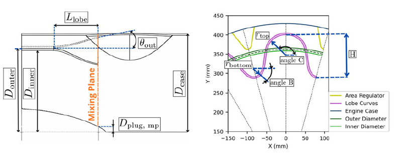
Lateral view of the geometry (left) and view of the lobed profile at the mixing plane (right).

Figure 1. Long description
A diagram of a coaxial mixer geometry. The diagram includes several labeled dimensions and angles. The outer diameter is labeled as D outer, the inner diameter as D inner, the case diameter as D case, and the plug diameter at the mixing plane as D plug, mp. The length of the lobe is labeled as L lobe, and the angle at the outlet is labeled as θ out. The mixing plane is indicated with an orange dashed line. The diagram shows the relationships between these dimensions and the overall structure of the coaxial mixer.
2.1 Geometry and meshing
The configuration object of this study is a 12-lobe mixer (see Figures 1 and 2) equipped with an area regulator that enables adjustment of the bypass-to-core area ratio at the mixing plane. This area regulator consists of 12 bumps that can move axially and slot into the mixer’s lobes. As such, the area regulator can only vary the bypass area, altering the total flow area at the mixing plane.
3D view of the Rear-VABI geometry.

Figure 2. Long description
Panel A: Perspective view of a coaxial mixer geometry. The structure features a central teal-colored sphere surrounded by a ring of yellow and purple lobes. Panel B: Lateral view of the coaxial mixer geometry. The central teal-colored sphere is visible along with the yellow and purple lobes arranged symmetrically around it. Panel C: Front view of the coaxial mixer geometry. The central teal-colored sphere is prominently displayed in the center, encircled by the yellow and purple lobes.
This geometry concept is proposed by Liu et al. [Reference Liu14]. Its advantages are that the moving parts are only exposed to the cold bypass flow and that the mechanical actuator structure is simple. Moreover, the characteristic lobe geometry enhances mixing by generating large-scale vortices at the trailing edge of the lobes. However, this shape increases the wetted surface area, leading to higher total pressure losses [Reference Huang17].
The geometry of a single lobe is defined through a set of characteristic parameters commonly adopted in previous studies [Reference Cooper, Merati and Hu18, Reference Salman, Page and McGuirk19]. These include the lobe height (
 $H$
), the number of lobes (
 $N$
) and the area ratio between bypass and core streams at the mixing plane (
 ${A_{{\rm b}}}/{A_{{\rm c}}}$
). The extent of the lobes in the axial direction is defined by (
 $L_{{\rm lobe}}$
), while the radial extent is defined by the penetration angle (
 $\theta$
).
Each half-lobe is modelled using two circular arcs describing the bottom and top parts of the profile, of radii
 $r_{{\rm bottom}}$
and
 $r_{{\rm top}}$
, connected by a Bézier curve to ensure tangency and geometric continuity. All geometric quantities are expressed as functions of prescribed design parameters, with the lobe height being a free variable. This parameter is computed iteratively to obtain a target area ratio between core and bypass areas at the mixing plane. This parametrisation allows the lobe geometry to be uniquely determined from a minimal set of input parameters and enables rapid generation of geometries that are consistent with prescribed flow-area constraints.
The area regulator profile at the mixing plane is fixed and is included in the bypass area calculation to ensure consistency with the imposed area ratio. It is defined by a circular arc of radius 21 mm and an angle of 18 degrees. This arc is then connected to the engine case by a straight line inclined at 81 degrees to the horizontal. The area regulator extends over an axial length of 400 mm. The lobes are integrated within a coaxial duct configuration defined by an inner diameter
 $D_{{\rm inner}}$
and an outer diameter
 $D_{{\rm outer}}$
. The difference between these diameters determines the local lobe thickness, which varies along the axial direction, from 8 mm at the duct junction to 4 mm at the trailing edge of the lobes. A central plug is included and is characterised by its diameter at the mixing plane
 $D_{{\rm plug, \, mp}}$
, and at the inlet section of 200 mm. The total axial length of the mixing chamber, measured from the inlet to the outlet plane, is 1,400 mm.
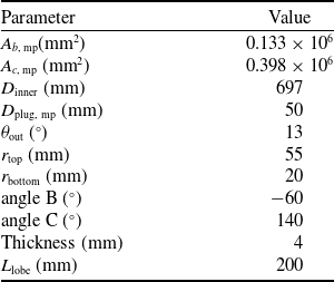
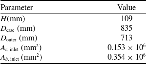
The values of the geometrical parameters are summarised in Table 1, while the corresponding geometric quantities computed by the geometry-generation tool are listed in Table 2. The geometric meaning of these parameters is illustrated in Figure 1.
Inputs of the geometry generation tool

Table 1. Long description
A table with two columns: Parameter and Value. The table has 11 rows, each listing a different geometrical parameter and its corresponding value. The parameters include Ab, mp, Ac, mp, D inner, D plug, mp, theta dat, r top, r bottom, angle B, angle C, Thickness, and L lobe, with values ranging from -60 to 0.398 times 10 to the power of 6.
Outputs of the geometry generation tool

Table 2. Long description
A table with two columns and five rows. The first column is labeled ‘Parameter’ and the second column is labeled ‘Value’. The table lists the following parameters and their corresponding values: H (mm) with a value of 109, D case (mm) with a value of 835, D outer (mm) with a value of 713, A c, inlet (mm^2) with a value of 0.153 x 10^6, and A b, inlet (mm^2) with a value of 0.354 x 10^6.
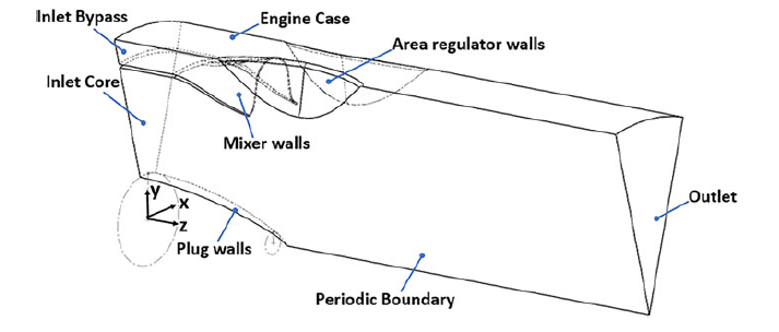
Given the geometric periodicity, a domain containing a single lobe was selected for the CFD study, with periodic boundary conditions applied on the lateral planes. A representation of the domain, containing a single 30-degree sector, is shown in Figure 3.
Computational domain for the numerical simulations.

Figure 3. Long description
A diagram of a coaxial mixer used in engineering applications. The diagram includes labeled parts such as Inlet Bypass, Inlet Core, Engine Case, Area Regulator Walls, Mixer Walls, Plug Walls, Periodic Boundary, and Outlet. The structure shows the flow from the Inlet Bypass and Inlet Core through the Engine Case, passing through the Area Regulator Walls and Mixer Walls, and finally exiting at the Outlet. The Plug Walls and Periodic Boundary are also indicated in the diagram. The diagram includes a coordinate system with axes labeled X, Y, and Z.
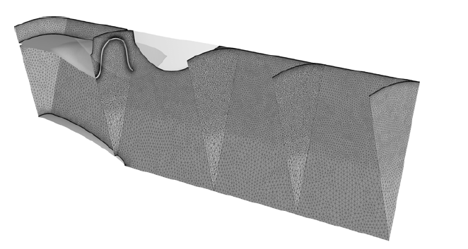
The computational domain is discretised using an unstructured mesh with localised volume refinement downstream of the lobe. The boundary layer first cell height is imposed equal to
 $2 \times 10^{-6}$
m to maintain a wall y + value below 1, thereby fully resolving the viscous sublayer. Twenty-seven prismatic layers are used, with a growth rate of 1.25, ending with a total inflation layer thickness of approximately 1.7 mm, which smoothly transitions to the core mesh.
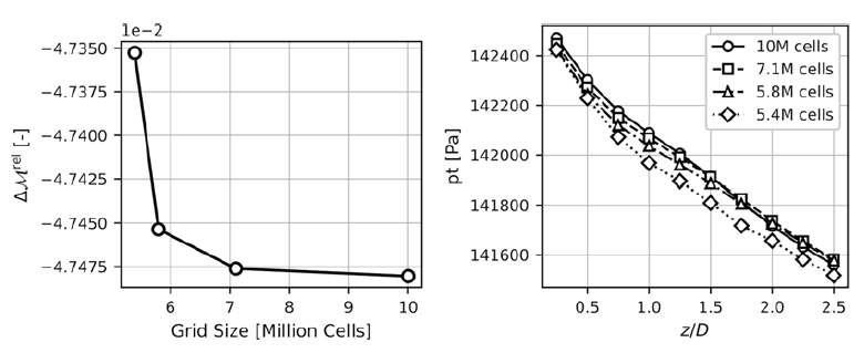
Mesh convergence trend of the relative momentum difference (left) and total pressure at different axial positions (right).

Mesh selected during the mesh convergence study.

A mesh independence study was performed to determine the minimum grid resolution, which provides mesh-independent results at an acceptable computational cost. Four meshes were generated by scaling an initial mesh using cell length multipliers of 2, 1, 0.7 and 0.5. The reference mesh sizes were 0.015 m for the global mesh and 0.009 m and 0.008 m for two local refinement regions. Mesh convergence was assessed in terms of the axial total pressure evolution and the relative momentum difference between inlets and outlets, as defined by Equations (1) and (2). The results of the mesh convergence study are shown in Figure 4. Based on these results, the mesh with a multiplier of 0.7 (7.1 million cells) provides a satisfactory trade-off between accuracy and cell count. The final mesh is depicted in Figure 5.
 \begin{align} \Delta \mathcal{M}^{{\rm rel}}=\frac {\mathcal{M}_{{\rm in}} - \mathcal{M}_{{\rm out}}} {\mathcal{M}_{{\rm in}}} \\[-10pt] \nonumber \end{align}
 \begin{align} \mathcal{M} = \int _{A} \rho v^2 \, {\rm d}A + \int _{A} p \, {\rm d}A \\[2pt] \nonumber \end{align}
2.2 Numerical setup and boundary conditions
The simulations are performed using the ANSYS Fluent 2024R2 pressure-based solver, which is suitable for simulating flows in the compressible subsonic regime experienced in this study [Reference Van den Borre, Saracoglu and Coussement20, Reference Zore21]. The working fluid is treated as an ideal gas with properties corresponding to air. The contribution of combustion products to the core-stream composition is neglected. This approximation primarily influences thermophysical properties, including the specific heat and the specific gas constant. The resulting impact on the VABI performance is expected to be minor and is therefore omitted from the present analysis.
Convective terms are discretised using a second-order upwind scheme. Pressure–velocity coupling is achieved using the coupled algorithm. The energy equation is enabled to account for compressibility effects, which become significant at the flow velocities encountered in the VABI, reaching up to Mach 0.5. Density is updated iteratively using the ideal gas law. The realisable k-
 $\epsilon$
model is selected as the turbulence model, which, as will be demonstrated in the validation (Section 2.3), has shown the closest match to experimental results for similar turbulent mixing cases. Turbulence levels at the inlets are estimated at 3% for the fan flow and 5% for the turbine flow. The boundary conditions consist of total pressure and temperature at the inlets, static pressure at the outlet and periodic boundary conditions on the sector faces to exploit the geometry’s periodicity. All walls have the no-slip condition applied.
2.3 Validation of lobed mixers
To validate the RANS approach, a comparison was performed between the numerical results and the experimental investigation of Hu et al. [Reference Hu7], which examines the flow field of an air jet discharged into the ambient environment through a lobed nozzle. Three different turbulence models have been assessed:
 $ k$
-
 $\varepsilon$
realisable,
 $ k$
−
 $\omega$
shear strain turbulence (SST) model and Spalart–Allmaras.
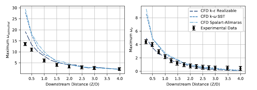
Validation of the model: decay along the streamwise direction of the maximum streamwise and azimuthal vorticity.

Figure 6. Long description
Two line graphs compare computational fluid dynamics models with experimental data. Panel A: The line graph shows the maximum azimuthal vorticity as a function of downstream distance. The x-axis is labeled ‘Downstream Distance (Z/D)’ and ranges from 0 to 4. The y-axis is labeled ‘Maximum ω azimuthal’ and ranges from 0 to 30. Three different computational fluid dynamics models (k-ε Realizable, k-ω SST, and Spalart-Allmaras) are represented by dashed lines, and experimental data is shown with black squares. The graph shows a decreasing trend in maximum azimuthal vorticity with increasing downstream distance. Panel B: The line graph shows the maximum streamwise vorticity as a function of downstream distance. The x-axis is labeled ‘Downstream Distance (Z/D)’ and ranges from 0 to 4. The y-axis is labeled ‘Maximum ω_z’ and ranges from 0 to 8. Similar to Panel A, three different computational fluid dynamics models are represented by dashed lines, and experimental data is shown with black squares. The graph shows a decreasing trend in maximum streamwise vorticity with increasing downstream distance.
Quantitative comparisons between numerical predictions and DP-SPIV measurements show good overall agreement for peak streamwise (
 $\omega _z$
) and azimuthal (
 $\omega _{{\rm azimuthal}}$
) vorticity (Figure 6). For azimuthal vorticity, all models fall within experimental uncertainty beyond
 $Z/D = 2$
, whereas upstream the Spalart–Allmaras and
 $k$
–
 $\omega$
SST models overpredict by up to 118%, compared to about 42% for the realisable
 $k$
–
 $\varepsilon$
model. A similar trend is observed for streamwise vorticity: agreement is reached beyond
 $Z/D = 1.75$
, while closer to the nozzle deviations increase to 111% for the Spalart–Allmaras and
 $k$
–
 $\omega$
SST models, but remain within 14% for the realisable
 $k$
–
 $\varepsilon$
model. Overall, the realisable
 $k$
–
 $\varepsilon$
model shows the best agreement, indicating that a RANS approach with a two-equation turbulence model captures the dominant flow features.
2.4 Results
To generate the performance map for the VABI, numerical simulations are performed with boundary conditions imposed to replicate the thermodynamic states encountered during typical engine operation. The operability of the VABI was investigated over a range of area ratios
 $A_{{\rm b}}/A_{{\rm c}}$
between 0.255 and 0.376, corresponding to different axial positions of the area regulator. The simulations were performed for inlet total pressure ratios
 $p_{{\rm t, \, b}}/p_{{\rm t, \, c}}$
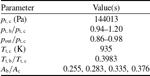
varying from 0.94 to 1.20 and for static outlet to total core inlet pressure ratios spanning from 0.86 to 0.98. The boundary conditions employed in this study are summarised in Table 3.
Parameter values for the test matrix

Table 3. Long description
A table listing parameter values for a test matrix. The table has two columns: Parameter and Value(s). It contains six rows with the following data: Row 1: Parameter, p_t,c (Pa); Value(s), 144013. Row 2: Parameter, p_t,b/p_t,c; Value(s), 0.94-1.20. Row 3: Parameter, p_out/p_t,c; Value(s), 0.86-0.98. Row 4: Parameter, T_t,c (K); Value(s), 935. Row 5: Parameter, T_t,b/T_t,c; Value(s), 0.3983. Row 6: Parameter, A_b/A_c; Value(s), 0.255, 0.283, 0.335, 0.376.
Figure 7 illustrates the development of the flow along the axial direction for the case with
 $A_{{\rm b}}/A_{{\rm c}}=0.335$
,
 $p_{{\rm t, \, b}}/p_{{\rm t, \, c}}=1.00$
and
 $p_{{\rm out}}/p_{{\rm t, \, c}}=0.86$
. The flow evolution is visualised along a series of cross-sectional planes located at different axial positions downstream of the mixing plane. The plane locations are normalised between the mixing plane (
 $z/L=0$
) and the mixer exit (
 $z/L=1$
). This figure shows how the vortices generated by the lobes mix the slower bypass flow into the faster core flow.
Axial evolution of the flow field, visualised on multiple cross-sectional planes at increasing downstream locations.

Figure 7. Long description
A cross-sectional view of a flow field in an aircraft engine, showing velocity magnitude at different downstream locations. The image displays multiple cross-sectional planes at increasing downstream locations, labeled from 0 to 1.0. The velocity magnitude is color-coded, ranging from blue (0 m/s) to red (348 m/s). The flow field exhibits complex patterns, with swirling and turbulent regions visible in the cross-sections. The image highlights the variability in flow characteristics as the air moves through the engine components.
Contours of Mach,
 $\omega _z$
and total temperature fields for the cases defined in Table 4.

Figure 8. Long description
The image contains four sets of contour plots, each set showing three different fields: Mach number, streamwise vorticity, and total temperature. Each set is labeled (a), (b), (c), and (d). The Mach number contours range from 0.0 to 0.6, with colors transitioning from black to red. The streamwise vorticity contours range from -3000 to 3000 1/s, with colors transitioning from blue to red. The total temperature contours range from 331 to 939 K, with colors transitioning from blue to red. Panel (a): The Mach number contours show a gradient from black to red, indicating increasing Mach numbers. The streamwise vorticity contours display alternating blue and red regions, indicating vorticity patterns. The total temperature contours show a mix of blue and red regions, indicating varying temperatures. Panel (b): Similar to Panel (a), the Mach number contours show a gradient from black to red. The streamwise vorticity contours display more pronounced blue and red regions. The total temperature contours show a more distinct pattern of blue and red regions. Panel (c): The Mach number contours are predominantly gray, indicating lower Mach numbers. The streamwise vorticity contours show less pronounced blue and red regions. The total temperature contours display a mix of blue and red regions. Panel (d): The Mach number contours show a gradient from black to red, similar to Panel (a). The streamwise vorticity contours display alternating blue and red regions. The total temperature contours show a mix of blue and red regions, indicating varying temperatures.
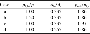
Figure 8 displays the contours of Mach number, streamwise vorticity and total temperature for four operating conditions. The operating conditions are summarised in Table 4, and the streamwise vorticity is defined as:
 \begin{align} \omega _z = \left ( \frac {\partial v}{\partial x} - \frac {\partial u}{\partial y} \right ) \ \end{align}
The vorticity field, presented in Figure 8, highlights the development of the shear layer and the formation of large-scale vortical structures downstream of the mixer trailing edge. The lobed shape of the mixer induces strong rotational motion, promoting momentum exchange between the core and bypass streams and enhancing mixing, leading to a more uniform distribution of thermodynamic quantities at the outlet. The vorticity colour scale ranges from
 $-3,000$
to
 $3,000$
, where positive values (red) denote counter-clockwise rotating structures and negative values (blue) indicate clockwise rotation, as viewed in the downstream direction.
A comparison between cases a and c shows that increasing the outlet static pressure primarily reduces the momentum of both streams, resulting in lower Mach numbers and lower streamwise vorticity levels, while the vortical structure shape remains unchanged. In contrast, increasing the inlet total pressure ratio (case b) increases the mass flow rate of the bypass stream with respect to the core stream, leading to higher local Mach numbers but reduced mixing efficiency, as evidenced by a less uniform total temperature distribution at the outlet compared to the reference case. Finally, reducing the bypass area (case d) significantly alters the spatial development of the vortical structures, thereby modifying the downstream evolution of the flow field and associated thermodynamic quantities.
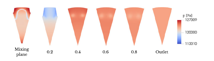
Figure 9 displays the static pressure distribution for case a. A common assumption in the literature for modelling the rear VABI, or a conventional constant-area duct mixer, is that the two streams have equal static pressure at the mixing plane. This hypothesis corresponds to the ideal case, where all flow is axial, and is used in zero-dimensional mixer models, as it provides a closure equation for determining the bypass flow rate. However, this assumption may not hold for a highly three-dimensional flow, such as that which develops in a lobed mixer. Indeed, the vortices generated by the lobes lead to curvature in the streamlines, which generate a pressure gradient in the direction normal to the streamline towards the local radius of curvature, though the streamline curvature equation:
 \begin{align} \frac {\partial p}{\partial n} = \rho \frac {v^2}{R} \end{align}
with
 ${\partial p}/{\partial n}$
the pressure gradient normal to the streamline in the direction of the local curvature,
 $v$
the velocity and
 $R$
the radius of the streamline curvature. The results, as seen in Figure 9, show that static-pressure equilibrium is indeed not achieved immediately at the mixer trailing edge, with the presence of high-pressure zones near the walls. Furthermore, two low-pressure zones remain at the centres of the vortices generated by the lobes, which don’t dissipate before reaching the mixer exit, where a uniform static pressure balance is imposed. This observation is consistent with the findings of Huang et al. [Reference Huang17], which state that static-pressure equivalence occurs only when the velocity component perpendicular to the axial direction becomes negligible. In the present configuration, the mixer geometry is specifically designed to promote radial transport, and a static-pressure mismatch between the streams is expected. Finally, observing Figure 9, a sudden static pressure drop can be noticed at
 $z/L = 0.2$
. This drop occurs in correspondence with the area regulator, whose presence reduces the flow passage area. As a result, the flow accelerates, leading to a static pressure drop.
Boundary conditions of the cases depicted in Figure 8

Table 4. Long description
A table comparing boundary conditions for different cases. The table has four rows and three columns. The columns are labeled as P_t,b/P_t,c, A_b/A_c, and P_out/P_t,c. The rows are labeled as Case a, Case b, Case c, and Case d. Row 1: Case a, P_t,b/P_t,c 1.00, A_b/A_c 0.335, P_out/P_t,c 0.86. Row 2: Case b, P_t,b/P_t,c 1.20, A_b/A_c 0.335, P_out/P_t,c 0.86. Row 3: Case c, P_t,b/P_t,c 1.00, A_b/A_c 0.335, P_out/P_t,c 0.97. Row 4: Case d, P_t,b/P_t,c 1.00, A_b/A_c 0.255, P_out/P_t,c 0.86.
3.0 Reduced order mixer model
A VABI performance map must characterise the component across its operating envelope: for any given set of input parameters, a unique operating point is identified, and the corresponding performance metrics can be retrieved. The rear-VABI has two thermodynamic inlets and one thermodynamic outlet. The following six parameters fully describe the thermodynamic state at both inlets, the position of the area regulator and the mass flow rate through the VABI:
 \begin{align} \frac {p_{{\rm t, \, b}}}{p_{{\rm t, \, c}}}, \quad \frac {p_{{\rm out}}}{p_{{\rm t, \, c}}}, \quad \frac {T_{t,\, b}}{T_{t, \, c}}, \quad p_{{\rm t, \, c}}, \quad T_{t, \, c}, \quad \frac {A_{{\rm b}}}{A_{{\rm c}}} \end{align}
Static pressure distribution for case a in Table 4.

The total thermodynamic state in the core inlet is directly imposed by
 $p_c$
and
 $T_c$
. Combined with
 ${p_{{\rm t, \, b}}}/{p_{{\rm t, \, c}}}$
and
 ${T_{t,\, b}}/{T_{t, \, c}}$
, also the bypass inlet is completely defined.
 $A_{{\rm b}}/A_{{\rm c}}$
defines the setting of the area regulator, which would not be present in a conventional, fixed-geometry mixer. The mass flow rates are indirectly determined by
 $p_{{\rm exit}}/p_{{\rm t, \, c}}$
, with a lower value of
 $p_{{\rm exit}}/p_{{\rm t, \, c}}$
leading to higher mass flow rates. For the performance map, it is beneficial to use
 $\, \dot{\kern-1pt m}_c$
instead of
 $p_{{\rm out}}/p_{{\rm t, \, c}}$
, as
 $p_{{\rm out}}$
is an output of a system-level component model and, as such, not directly accessible, unlike an inlet mass flow rate.
The performance of the VABI component can be described by a set of non-dimensional and reduced parameters (also called corrected parameters). By doing so, the VABI’s performance collapses to a single value across different absolute input parameters, provided the corrected parameters are kept constant. This reduces the number of input parameters required to fully describe the VABI’s state, lowering the map’s dimensionality and the number of expensive, high-fidelity simulations needed to sample a given coverage. A similar procedure is employed to generate performance maps for compressors and turbines [Reference Kurzke and Halliwell9]. The following non-dimensional and corrected parameters are used to describe the performance map:
 \begin{align} \frac {p_{{\rm t, \, b}}}{p_{{\rm t, \, c}}}, \quad \, \dot{\kern-1pt m}_{{\rm corr}, \, c}, \quad \frac {A_{{\rm b}}}{A_{{\rm c}}} \end{align}
with the core-corrected core mass flow rate
 $\, \dot{\kern-1pt m}_{{\rm corr}, \, c}$
being defined as:
 \begin{align} \, \dot{\kern-1pt m}_{{\rm corr}, \, c} = \frac {\, \dot{\kern-1pt m}_c\sqrt {(T_{t, \, c}\ R)/(T_{t,\, ref} \ R_{ref})}}{p_{{\rm t, \, c}}/p_{t,\, ref}} \end{align}
Having defined the input parameters for the map, the output parameters that characterise the component performance need to be selected. The performance of the rear-VABI is primarily assessed using two metrics: its flow regulation ability, and the pressure losses in the system [Reference Koutmos and McGuirk16, Reference Xu22, Reference Song23]. Flow regulation capability is defined as the degree to which geometric variations of the VABI control the bypass mass flow fraction entering the component. Flow regulation capability can be quantified through quantities as the bypass ratio, defined as the ratio between bypass and core mass flow rates
 ${\rm BPR}={\, \dot{\kern-1pt m}_{b}}/{\, \dot{\kern-1pt m}_{c}}$
, or the absolute mass flow rates that enter the system. Given that the core mass flow rate is already used as an input for the map, the bypass mass flow rate is selected as the relevant performance parameter.
Total pressure loss characterises the aerodynamic efficiency of the component and the mixing process. Pressure losses in a mixing process arise from wall friction, flow separation, and entropy generation. A parameter generally used to quantify this loss is the total pressure loss coefficient, defined as:
 \begin{align} \sigma = \frac {\frac {1}{m_{{\rm out}}} \int p_{{\rm t, \, out}} \, {\rm d} m_{{\rm out}}}{\frac {1}{m_{{\rm in}}} \int p_{{\rm t,in}} \, {\rm d} m_{{\rm in}}} \end{align}
where the numerator represents the outlet mass flow-averaged total pressure
 $ p_{{\rm t, \, out}}$
, while the denominator corresponds to the equivalent mass-flow-averaged inlet total pressure.
3.1 Choice of the outlet parameters and validation of the map
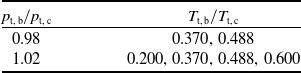
An assumption commonly used in the literature is to neglect the influence of the total temperature ratio on the performance parameters of the VABI, assuming the other non-dimensional parameters will have a stronger effect [Reference Xu22, Reference Song23]. To assess the validity of this assumption, additional simulations were conducted with varying inlet total temperature ratios while maintaining all other boundary conditions constant. The investigated operating points are summarised in Table 5. Two inlet total pressure ratios
 $ p_{{\rm t, \, b}}/p_{{\rm t, \, c}}$
were tested, and for each case, a characteristic curve was generated by systematically varying
 $ p_{{\rm out}}/p_{{\rm t, \, c}}$
.
Test matrix for the sensitivity analysis of inlet total temperature ratio effects on rear-VABI performance

Table 5. Long description
A table with two columns and two rows. The first column is labeled ‘P_l_b/P_l_c’ and the second column is labeled ‘T_l_b/T_l_c’. The table presents the following data: Row 1: P_l_b/P_l_c, 0.98; T_l_b/T_l_c, 0.370, 0.488. Row 2: P_l_b/P_l_c, 1.02; T_l_b/T_l_c, 0.200, 0.370, 0.488, 0.600.
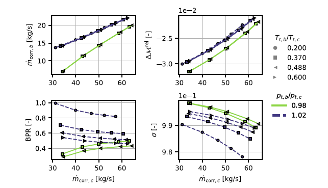
Sensitivity of the performance parameters of interest to variations in the inlet total temperature ratio for two constant inlet total pressure ratios.

Figure 10. Long description
The image contains four line graphs, each illustrating different performance parameters against corrected mass flow rate. Panel A shows the corrected mass flow rate on the vertical axis in kilograms per second and corrected mass flow rate on the horizontal axis in kilograms per second. Panel B depicts the relative Mach number difference with the same horizontal axis. Panel C illustrates the bypass pressure ratio with the same horizontal axis. Panel D shows the standard deviation with the same horizontal axis. Each graph includes data series differentiated by markers and colors, representing different ratios of inlet total temperature and inlet total pressure. The trends indicate how these performance parameters vary with changes in the corrected mass flow rate and the ratios of inlet total temperature and pressure.
The sensitivity analysis results, depicted in Figure 10, reveal that both the bypass ratio and pressure loss coefficient exhibit significant dependence on
 ${T_{t,\, b}}/{T_{t, \, c}}$
, demonstrating that the temperature ratio independence assumption is not valid for these performance parameters. Two alternative parameters, also depicted in Figure 10, show negligible
 ${T_{t,\, b}}/{T_{t, \, c}}$
sensitivity, while adequately representing flow regulation and total pressure losses. The first one is the corrected bypass mass flow rate (
 $\, \dot{\kern-1pt m}_{{\rm corr}, \, b}$
). The second is the relative momentum difference between the inlet and outlet, calculated as in Equation (1). The momentum
 $\mathcal{M}$
is defined with Equation (2) that applied to a one-dimensional flow aligned with the axial direction, and considering the inlet and outlet of the VABI, develops in:
 \begin{align} \mathcal{M}_{{\rm in}} &= v_{{\rm c}}\,\, \dot{\kern-1pt m}_{{\rm c}} + v_{{\rm b}}\,\, \dot{\kern-1pt m}_{{\rm b}} + A_{{\rm c}}\,p_{{\rm c}} + A_{{\rm b}}\,p_{{\rm b}} \end{align}
 \begin{align} \mathcal{M}_{{\rm out}} &= v_{{\rm out}}\,\, \dot{\kern-1pt m}_{{\rm out}} + A_{{\rm out}}\,p_{{\rm out}} \end{align}
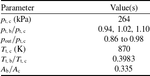
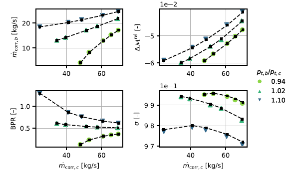
To verify that the component behaviour depends only on non-dimensional parameters and not on absolute thermodynamic state, additional CFD simulations were performed at some selected map operating points. These simulations use different absolute inlet total pressures than those used to create the original map, while maintaining identical non-dimensional input parameters. A summary of the values used for these simulations is shown in Table 6. Figure 11 presents a comparison between the original performance map data (coloured scattered points) and the validation simulation results (black points connected by dashed lines).
Test matrix used for validation of map independence from absolute thermodynamic state

Table 6. Long description
A table with two columns and seven rows. The first column is labeled ‘Parameter’ and the second column is labeled ‘Value(s)’. The parameters and their corresponding values are as follows: Row 1: p_t,c (kPa), 264. Row 2: p_t,b/p_t,c, 0.94, 1.02, 1.10. Row 3: p_out/p_t,c, 0.86 to 0.98. Row 4: T_t,c (K), 870. Row 5: T_t,b/T_t,c, 0.3983. Row 6: A_b/A_c, 0.335.
Verification of map independence from the absolute thermodynamic state through comparison with CFD simulations at identical non-dimensional inputs and different absolute pressure levels. Performed at
 $A_{{\rm b}}/A_{{\rm c}}=0.335$
.

Figure 11. Long description
The image contains four line graphs, each illustrating different relationships between variables in aircraft engine simulations. Panel A: The line graph shows the corrected mass flow rate on the y-axis in kilograms per second against the corrected mass flow rate on the x-axis in kilograms per second. Different markers and colors represent various pressure ratios. The lines indicate increasing trends for different pressure ratios. Panel B: The line graph depicts the relative change in a variable on the y-axis against the corrected mass flow rate on the x-axis in kilograms per second. Different markers and colors represent various pressure ratios, showing increasing trends. Panel C: The line graph shows the bypass ratio on the y-axis against the corrected mass flow rate on the x-axis in kilograms per second. Different markers and colors represent various pressure ratios, indicating decreasing trends. Panel D: The line graph depicts a variable on the y-axis against the corrected mass flow rate on the x-axis in kilograms per second. Different markers and colors represent various pressure ratios, showing varying trends.
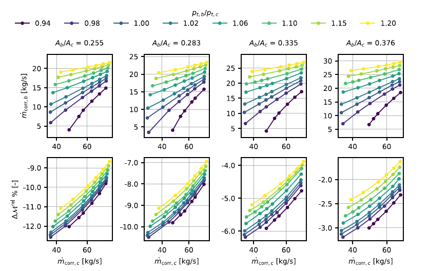
The close match between the tested points and the map curves confirms that the proposed parameter reduction is effective, with performance independent of the absolute thermodynamic state within the investigated range. Therefore, it can be applied as long as the non-dimensional input parameters lie within the map bounds. The complete rear-VABI performance map, expressed in terms of the selected input and output parameters, is presented in Figure 12. The performance characteristics are expressed in terms of
 $\, \dot{\kern-1pt m}_{_{{\rm corr}, \, b}}$
and
 $\Delta \mathcal{M}^{{\rm rel}}$
. The latter is shown in percentage. The performance map shows that increasing
 $A_{{\rm b}}/A_{{\rm c}}$
moves the operation toward higher corrected bypass mass flow rates. The relative momentum difference is defined as the normalised difference between inlet and outlet momentum. Its negative values indicate a net momentum gain from inlet to outlet, which arises because the sum of
 $A_b$
and
 $A_c$
does not equal
 $A_{out}$
due to the presence of the area regulator and the plug. The momentum gain due to area change consistently exceeds friction losses, keeping
 $\Delta \mathcal{M}^{{\rm rel}}$
negative throughout the map. Three trends can be observed in the momentum loss distribution shown in the map. First, at fixed area ratio,
 $\Delta \mathcal{M}^{{\rm rel}}$
increases in magnitude with increasing mass flow rate: higher corrected mass flow rates result from lower back pressure, which raises flow velocities and pressure losses, while the area-induced momentum gain remains constant. Second, increasing total pressure ratio at fixed area ratio leads to higher momentum losses. Third, higher area ratios produce higher momentum loss. This is attributed to the increased bypass mass flow entering the system at higher
 $A_{{\rm b}}/A_{{\rm c}}$
, which intensifies core-bypass mixing and the associated losses, outweighing the reduction in area-induced momentum gain from the larger inlet area.
Full performance map of the VABI.

4.0 Demonstration of the VABI in a three-stream engine
In this section, the results of the CFD simulations are used to create a reduced-order VABI model in Modelon Impact. This model is used in a notional three-stream VCE to study the effect of the VABI area regulator position on the engine performance and flow-holding capabilities.
4.1 Practical implementation in Modelon Impact
The performance maps extracted from the CFD simulations are used to construct a VABI model in Modelon Impact [24], which is built on the Modelica language [25], an acausal, equation-based, object-oriented programming language designed for physical system modelling. Unlike causal languages, Modelica represents physical systems as sets of differential-algebraic equations (DAEs) without predefined input–output causality. Once a model is constructed, Modelon Impact compiles it using the Optimica Compiler Toolkit (OCT) [Reference Modelon26], which symbolically processes the Modelica equations, performs index reduction for DAEs and generates an executable representation in the form of a Functional Mock-up Unit (FMU) [27]. For steady-state analysis, the problem reduces to solving a nonlinear algebraic system:
 \begin{align} \textbf{R}(\textbf{x}) = \textbf{0} \end{align}
where
 $\textbf{x}$
denotes the vector of iteration variables (IVs), and
 $\textbf{R}\left (\textbf{x}\right )$
represents the residual equations derived from component matching and system constraints. In the context of gas turbine modelling, typical IVs include spool speeds (
 $N_L, N_H$
) and turbomachinery matching parameters such as R-lines. The residual equations enforce conditions such as shaft torque balance, mass-flow compatibility and thermodynamic closure. The nonlinear system is solved using a solver based on Krylov Inexact Newton SOLver (KINSOL), part of the SUite of Nonlinear and DIfferential/ALgebraic equation Solvers (SUNDIALS) suite [Reference Hindmarsh28]. The solver implements a Newton-based method with advanced features, such as line search, damping strategies and preconditioned iterative linear solvers, to improve robustness and convergence. At each iteration, the solver updates IVs by approximately solving:
 \begin{align} \textbf{x}^{(k+1)} = \textbf{x}^{(k)} - \textbf{J}^{-1}(\textbf{x}^{(k)}) \, \textbf{R}(\textbf{x}^{(k)}) \end{align}
where
 $\textbf{J} = \frac {\partial \textbf{R}}{\partial \textbf{x}}$
is the Jacobian of residuals with respect to IVs. Convergence is achieved when the residual norm falls below a specified tolerance, ensuring all matching conditions are satisfied simultaneously.
For jet engine simulations, mixer component calculations involve two phases: on-design and off-design. In the on-design phase, all engine design parameters, such as compressor pressure ratios, bypass ratio and mass flow ratio, are freely specified by the designer and imposed on the engine components. With these imposed parameters, each component is sized, which includes both the physical sizing of flow areas and the scaling of performance maps. For a conventional mixer component, this involves sizing inlet areas to meet a specific design Mach number, typically that of the core flow at the mixing plane. This procedure introduces three IVs: core area, bypass area and total exit pressure. These IVs are solved against residual equations enforcing core Mach number, static pressure balance at the mixing plane and momentum balance over the mixer, respectively. In the off-design phase, the inlet areas are fixed, with the IVs changing to bypass mass flow rate and total exit pressure, with residuals enforcing static pressure and momentum balance.
For the VABI developed in this work, the procedure differs. The residual equations derived from static pressure and momentum balance in a constant-area duct are replaced by residuals based on performance map continuity. Three maps are considered:
-
• Relative momentum difference map
-
• Bypass corrected mass flow map
-
• Core corrected mass flow map
Each map uses the same three input parameters:
 $\beta$
,
 $p_{{\rm t, \, b}}/p_{{\rm t, \, c}}$
and
 $A_{{\rm b}}/A_{{\rm c}}$
. Ideally,
 $\, \dot{\kern-1pt m}_{{\rm corr}, \, c}$
would be used directly as an input, but trilinear interpolation requires a rectilinear grid in the input space, which is not achievable for
 $\, \dot{\kern-1pt m}_{{\rm corr}, \, c}$
, given the CFD sampling strategy. Consequently, an artificial parameter
 $\beta$
is introduced, varying from 0 to 1 in fixed steps. This
 $\beta$
becomes an IV, iterated until the desired
 $\, \dot{\kern-1pt m}_{{\rm corr}, \, c}$
is achieved, forming a first IV-residual pair.
The second IV–residual pair consists of the outlet total pressure, which is varied until the following momentum balance equation is satisfied:
 \begin{align} \big ( 1 - \Delta \mathcal{M}^{{\rm rel}} \big) \bigl [ \left ( \, \dot{\kern-1pt m} v + pA \right )_c +\left ( \, \dot{\kern-1pt m} v + pA \right )_b \bigr ] &= \left ( \, \dot{\kern-1pt m} v + pA \right )_e \end{align}
For the third pair, the on- and off-design behaviour is different. For on-design, the complete state for the inlets, including
 $p_{{\rm t, \, b}}/p_{{\rm t, \, c}}$
and
 $\, \dot{\kern-1pt m}_{{\rm corr}, \, b}$
, is defined by the engine design parameters. As
 $\beta$
is already used for the matching of
 $\, \dot{\kern-1pt m}_{{\rm corr}, \, c}$
, that only leaves the map input parameter
 $A_{{\rm b}}/A_{{\rm c}}$
available to be used as IV. The
 $A_{{\rm b}}/A_{{\rm c}}$
that solves the
 $\, \dot{\kern-1pt m}_{{\rm corr}, \, b}$
continuity equation will be defined as the design area ratio, forming the default area regulator position. In off-design,
 $\, \dot{\kern-1pt m}_{{\rm corr}, \, b}$
is no longer imposed, but will result from the off-design matching of the turbomachinery. This adds one degree of freedom, which allows to impose
 $A_{{\rm b}}/A_{{\rm c}}$
as a control parameter. As such, the residual equation of
 $\, \dot{\kern-1pt m}_{{\rm corr}, \, b}$
continuity will be solved by an IV outside of the VABI component from an engine system level.
4.2 Simulation results in a notional three-stream VCE
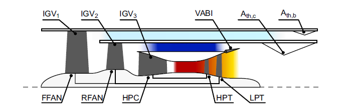
The VABI model is demonstrated in a notional three-stream VCE architecture. A schematic representation of the VCE is shown in Figure 13. The configuration consists of a core stream, a mixed bypass stream (inner bypass) and an unmixed bypass stream (outer bypass). In the three-stream VCE, the VABI controls the inner bypass ratio.
Three-stream VCE used to demonstrate the VABI components in a system model.

Figure 13. Long description
A diagram of a three-stream VCE system demonstrating VABI components. The diagram includes labeled parts such as IGV1, IGV2, IGV3, VABI, A_th,c, A_th,b, FFAN, RFAN, HPC, HPT, and LPT. The flow starts from the left with the FFAN and RFAN, progresses through the HPC, and continues through the HPT and LPT. The VABI component is situated between the HPC and HPT sections. The diagram illustrates the interaction and flow between these components, with color gradients indicating different states or conditions within the system.
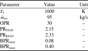
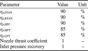
The engine design parameters and technology levels are summarised in Tables 7 and 8. These were selected such that the VABI map fits the engine without requiring scaling of corrected air flows or cross-sectional areas in the map. The design point is set at a flight Mach number of
 $0.8$
and an altitude of
 $10\,{\rm km}$
. A VCE of this type can include various variable geometries, such as nozzles, inlet guide vanes (IGVs), VABIs and nozzle guide vanes (NGVs) [Reference Johnson29]. However, for this demonstration, only the VABI is implemented.
Engine design parameters

Table 7. Long description
A table with six rows and three columns listing engine design parameters and their values. The columns are labeled Parameter, Value, and Unit. The parameters include T4, m_dot_air, OPR, PR_FFAN, PR_RFAN, BPR_outer, and BPR_inner. The values and units for each parameter are as follows: T4, 1600 K; m_dot_air, 95 kg/s; OPR, 30; PR_FFAN, 2.15; PR_RFAN, 2.33; BPR_outer, 0.08; BPR_inner, 0.40.
Engine technology limits

Table 8. Long description
A table summarizing engine design parameters and technology levels. The table has 6 rows and 3 columns. The columns are labeled Parameter, Value, and Unit. The rows are as follows: Row 1: Parameter, eta_p_FFAN; Value, 90; Unit, percent. Row 2: Parameter, eta_p_RFAN; Value, 90; Unit, percent. Row 3: Parameter, eta_p_HPC; Value, 90; Unit, percent. Row 4: Parameter, eta_p_HPT; Value, 85; Unit, percent. Row 5: Parameter, eta_p_LPT; Value, 85; Unit, percent. Row 6: Parameter, Nozzle thrust coefficient; Value, 1; Unit, empty. Row 7: Parameter, Inlet pressure recovery; Value, 1; Unit, empty.
Two engine models are produced:
-
• Reference engine: Implements the conventional static-pressure-balance VABI.
-
• Map-driven VABI engine: Implements the VABI using performance maps derived from CFD data.
After completing the on-design simulations, a series of throttle curves are generated for both engines under on-design flight conditions by performing a sweep on turbine inlet temperature (
 $T_4$
) between
 $900\,{\rm K}$
and
 $1,600\,{\rm K}$
. For the map-driven VABI engine, multiple curves are produced that correspond to VABI positions ranging from fully closed to fully open. These positions correspond to area ratios of
 $0.259$
and
 $0.370$
, respectively, with the latter coinciding with the design VABI position. For the reference engine, only the design VABI position is used, as the regulation would maintain a constant total mixing-plane area, invalidating a direct comparison.
Several performance indicators for the VCE as a function of thrust output and VABI position, indicated as area ratio at the mixing plane. The reference engine performance is indicated with the dashed line.

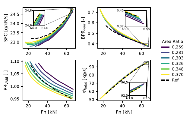
Figure 14 summarises the results, showing specific fuel consumption (SFC),
 ${\rm BPR}_{{\rm rear}}$
,
 ${\rm PR}_{{\rm VABI}}$
and inlet mass flow rate (
 $\, \dot{\kern-1pt m}_{{\rm inlet}}$
) as functions of uninstalled thrust output (
 $F_n$
). The VABI pressure ratio is defined as:
 \begin{align*} {\rm PR}_{{\rm VABI}} = \dfrac {p_{{\rm t, \, b}}}{p_{{\rm t, \, c}}}. \end{align*}
The rear bypass ratio increases sharply when the throttle is reduced for all curves, including the reference engine. The VABI position influences
 ${\rm BPR}_{{\rm rear}}$
as expected: more closed positions reduce the bypass ratio. However, the variation within the studied VABI positions is limited to
 $3.5\%$
at maximum throttle, with differences becoming larger at lower throttle settings. The reference engine exhibits distinctly different behaviour compared to the map-driven VABI engine, confirming once more that the static pressure balance assumption is not valid for the considered VABI geometry.
All cases show an increase of
 ${\rm PR}_{{\rm VABI}}$
as the throttle is reduced. Across all curves,
 ${\rm PR}_{{\rm VABI}}$
approaches
 $1.1$
, after which the engine model fails to converge.
 ${\rm PR}_{{\rm VABI}}$
and
 ${\rm BPR}_{{\rm rear}}$
are inversely related: as
 ${\rm BPR}_{{\rm rear}}$
decreases, the RFAN processes less air, reducing its power consumption. This surplus power is used to increase compression, raising
 ${\rm PR}_{{\rm VABI}}$
. Again, the reference engine shows different behaviour, reinforcing that the static pressure balance assumption is invalid.
One advantage often cited for VCE engines is their flow-holding capability, where intake mass flow remains high at low throttle to reduce installation losses [Reference Clark, Tai and Mavris30–Reference Zenkner32]. However, Figure 14 shows only a modest variation of the inlet mass flow rate (
 $\approx 1.0\%$
) as the VABI area ratio changes. Other variable geometries, such as changes in nozzle throat area, have been shown in the literature to have a much larger effect [Reference Van Den Borre and Saracoglu12, Reference Chen, Zhang and Tang33]. In this instance, the design area ratio corresponds to the most open position, and as such, only a closing is possible. Counterintuitively, closing the area regulator actually increases the mass flow rate through the engine. This is because the total pressure upstream of the core nozzle increases, which can force more airflow through the choked nozzle. The effect is small, however, as it is counterbalanced by a slight increase in total temperature, resulting from a decrease in BPR.
The SFC curves indicate that the efficiency bucket occurs at relatively low thrust (
 $\approx 20\,{\rm kN}$
). When the VABI closes, the
 ${\rm PR}_{{\rm VABI}}$
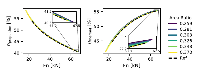
limit is often reached before this region. Nevertheless, closing the VABI improves the SFC under the given flight conditions. This is explained by Figure 15, which shows propulsion and thermal efficiency defined as:
 \begin{align} \eta _{{\rm thermal}} &= \frac {\, \dot{\kern-1pt m}_{{\rm n, \, c}} v_{{\rm n, \, c}}^2 + \, \dot{\kern-1pt m}_{{\rm n, \, b}} v_{{\rm n, \, b}}^2 - \, \dot{\kern-1pt m}_{{\rm amb}} v_{{\rm amb}}^2}{2 \dot {q}} \end{align}
 \begin{align} \eta _{{\rm propulsion}} &= 2 v_{{\rm amb}} \cdot \frac {\, \dot{\kern-1pt m}_{{\rm n, \, c}} v_{{\rm n, \, c}} + \, \dot{\kern-1pt m}_{{\rm n, \, b}} v_{{\rm n, \, b}} - \, \dot{\kern-1pt m}_{{\rm amb}} v_{{\rm amb}}}{\, \dot{\kern-1pt m}_{{\rm n, \, c}} v_{{\rm n, \, c}}^2 + \, \dot{\kern-1pt m}_{{\rm n, \, b}} v_{{\rm n, \, b}}^2 - \, \dot{\kern-1pt m}_{{\rm amb}} v_{{\rm amb}}^2} \end{align}
with the subscripts “n, b”, “n, c” and “amb” referring to bypass nozzle exit, core nozzle exit, and ambient flight conditions, respectively.
Propulsive and thermal efficiency of the VCE using the VABI map. The static-pressure-balance engine reference is shown as the dashed line.

Figure 15. Long description
Panel A: A line graph shows the propulsive efficiency (η_propulsion) in percent on the vertical axis and force (Fn) in kilonewtons on the horizontal axis. Multiple lines represent different area ratios, with a dashed line indicating a reference. The graph shows a decreasing trend in propulsive efficiency as force increases. Panel B: Another line graph displays thermal efficiency (η_thermal) in percent on the vertical axis and force (Fn) in kilonewtons on the horizontal axis. Similar to Panel A, multiple lines represent different area ratios, with a dashed line for the reference. This graph shows an increasing trend in thermal efficiency with increasing force. Both panels include insets that zoom in on specific data ranges.
Both efficiencies improve slightly when closing the VABI. Thermal efficiency increases with higher Overall Pressure Ratio (OPR). Closing the VABI increases nozzle exit velocities, thereby raising the propulsion efficiency and thrust. Combined with the downward slope of the propulsion efficiency curve, throttle curves for more closed VABI positions come out slightly ahead of more open ones. Lastly, the reference engine again shows a different SFC behaviour compared to the map-driven VABI engine.
5.0 Conclusion
This paper presented a methodology for generating a reduced-order model of a VABI based on high-fidelity numerical simulations and integrating it into system-level propulsion simulations. The approach establishes relationships between three non-dimensional input parameters and two key outputs: the corrected bypass mass flow rate and a loss metric derived from the relative momentum difference between the inlets and outlet.
From the high-fidelity analysis, two important findings emerge. First, the commonly used pressure loss coefficient exhibits a significant dependency on the inlet temperature ratio
 $T_{t,\, b}/T_{t, \, c}$
, which is often neglected in the literature. Secondly, the corrected bypass mass flow rate
 $\, \dot{\kern-1pt m}_{{\rm corr}, \, b}$
and the relative momentum difference
 $\Delta \mathcal{M}^{{\rm rel}}$
show negligible sensitivity to the temperature ratio when the other non-dimensional parameters are kept fixed, making them more representative for wider system simulations.
The assumption of static pressure balance at the mixing plane, widely adopted in conventional 0-D mixer models, was shown to be a strong simplification that deviates from the actual fluid-dynamic behaviour. An alternative methodology employing the VABI performance map was proposed and implemented in a notional three-stream variable-cycle engine. A comparison with a conventional mixer model revealed significant differences in off-design performance, indicating that the static-pressure balance assumption is inadequate for practical mixer geometries. Furthermore, the VABI demonstrated its ability to produce modest changes in engine bypass ratio (up to 4%), thereby influencing the throttle curves shape and specific fuel consumption (up to 1.3% at partial throttle).
Overall, the proposed methodology enables accurate integration of reduced-order VABI components into propulsion system simulations while reducing reliance on oversimplified assumptions, thereby improving fidelity in off-design performance prediction.
Acknowledgments
Funded by the European Union. Views and opinions expressed are, however, those of the authors only and do not necessarily reflect those of the European Union or the European Commission. Neither the European Union nor the granting authority can be held responsible for them. The authors would also like to thank the Modelon support received from Jim Claesson, head of Physics Engineering at Modelon AB and the support from professor Svend Bram at the Vrije Universiteit Brussel for proofreading the manuscript.



 ωz
 Ab/Ac=0.335

 Open access

