



%20--%3e%3c!DOCTYPE%20svg%20PUBLIC%20'-//W3C//DTD%20SVG%201.0//EN'%20'http://www.w3.org/TR/2001/REC-SVG-20010904/DTD/svg10.dtd'%3e%3csvg%20version='1.0'%20id='Layer_1'%20xmlns='http://www.w3.org/2000/svg'%20xmlns:xlink='http://www.w3.org/1999/xlink'%20x='0px'%20y='0px'%20width='64px'%20height='64px'%20viewBox='5.5%20-3.5%2064%2064'%20enable-background='new%205.5%20-3.5%2064%2064'%20xml:space='preserve'%3e%3cg%3e%3ccircle%20fill='%23FFFFFF'%20fill-opacity='0'%20cx='37.785'%20cy='28.501'%20r='28.836'/%3e%3cpath%20fill='%23595959'%20d='M37.441-3.5c8.951,0,16.572,3.125,22.857,9.372c3.008,3.009,5.295,6.448,6.857,10.314%20c1.561,3.867,2.344,7.971,2.344,12.314c0,4.381-0.773,8.486-2.314,12.313c-1.543,3.828-3.82,7.21-6.828,10.143%20c-3.123,3.085-6.666,5.448-10.629,7.086c-3.961,1.638-8.057,2.457-12.285,2.457s-8.276-0.808-12.143-2.429%20c-3.866-1.618-7.333-3.961-10.4-7.027c-3.067-3.066-5.4-6.524-7-10.372S5.5,32.767,5.5,28.5c0-4.229,0.809-8.295,2.428-12.2%20c1.619-3.905,3.972-7.4,7.057-10.486C21.08-0.394,28.565-3.5,37.441-3.5z%20M37.557,2.272c-7.314,0-13.467,2.553-18.458,7.657%20c-2.515,2.553-4.448,5.419-5.8,8.6c-1.354,3.181-2.029,6.505-2.029,9.972c0,3.429,0.675,6.734,2.029,9.913%20c1.353,3.183,3.285,6.021,5.8,8.516c2.514,2.496,5.351,4.399,8.515,5.715c3.161,1.314,6.476,1.971,9.943,1.971%20c3.428,0,6.75-0.665,9.973-1.999c3.219-1.335,6.121-3.257,8.713-5.771c4.99-4.876,7.484-10.99,7.484-18.344%20c0-3.543-0.648-6.895-1.943-10.057c-1.293-3.162-3.18-5.98-5.654-8.458C50.984,4.844,44.795,2.272,37.557,2.272z%20M37.156,23.187%20l-4.287,2.229c-0.458-0.951-1.019-1.619-1.685-2c-0.667-0.38-1.286-0.571-1.858-0.571c-2.856,0-4.286,1.885-4.286,5.657%20c0,1.714,0.362,3.084,1.085,4.113c0.724,1.029,1.791,1.544,3.201,1.544c1.867,0,3.181-0.915,3.944-2.743l3.942,2%20c-0.838,1.563-2,2.791-3.486,3.686c-1.484,0.896-3.123,1.343-4.914,1.343c-2.857,0-5.163-0.875-6.915-2.629%20c-1.752-1.752-2.628-4.19-2.628-7.313c0-3.048,0.886-5.466,2.657-7.257c1.771-1.79,4.009-2.686,6.715-2.686%20C32.604,18.558,35.441,20.101,37.156,23.187z%20M55.613,23.187l-4.229,2.229c-0.457-0.951-1.02-1.619-1.686-2%20c-0.668-0.38-1.307-0.571-1.914-0.571c-2.857,0-4.287,1.885-4.287,5.657c0,1.714,0.363,3.084,1.086,4.113%20c0.723,1.029,1.789,1.544,3.201,1.544c1.865,0,3.18-0.915,3.941-2.743l4,2c-0.875,1.563-2.057,2.791-3.541,3.686%20c-1.486,0.896-3.105,1.343-4.857,1.343c-2.896,0-5.209-0.875-6.941-2.629c-1.736-1.752-2.602-4.19-2.602-7.313%20c0-3.048,0.885-5.466,2.658-7.257c1.77-1.79,4.008-2.686,6.713-2.686C51.117,18.558,53.938,20.101,55.613,23.187z'/%3e%3c/g%3e%3c/svg%3e)
%20--%3e%3c!DOCTYPE%20svg%20PUBLIC%20'-//W3C//DTD%20SVG%201.0//EN'%20'http://www.w3.org/TR/2001/REC-SVG-20010904/DTD/svg10.dtd'%3e%3csvg%20version='1.0'%20id='Layer_1'%20xmlns='http://www.w3.org/2000/svg'%20xmlns:xlink='http://www.w3.org/1999/xlink'%20x='0px'%20y='0px'%20width='64px'%20height='64px'%20viewBox='5.5%20-3.5%2064%2064'%20enable-background='new%205.5%20-3.5%2064%2064'%20xml:space='preserve'%3e%3cg%3e%3ccircle%20fill='%23FFFFFF'%20fill-opacity='0'%20cx='37.637'%20cy='28.806'%20r='28.276'/%3e%3cg%3e%3cpath%20fill='%23595959'%20d='M37.443-3.5c8.988,0,16.57,3.085,22.742,9.257C66.393,11.967,69.5,19.548,69.5,28.5c0,8.991-3.049,16.476-9.145,22.456%20C53.879,57.319,46.242,60.5,37.443,60.5c-8.649,0-16.153-3.144-22.514-9.43C8.644,44.784,5.5,37.262,5.5,28.5%20c0-8.761,3.144-16.342,9.429-22.742C21.101-0.415,28.604-3.5,37.443-3.5z%20M37.557,2.272c-7.276,0-13.428,2.553-18.457,7.657%20c-5.22,5.334-7.829,11.525-7.829,18.572c0,7.086,2.59,13.22,7.77,18.398c5.181,5.182,11.352,7.771,18.514,7.771%20c7.123,0,13.334-2.607,18.629-7.828c5.029-4.838,7.543-10.952,7.543-18.343c0-7.276-2.553-13.465-7.656-18.571%20C50.967,4.824,44.795,2.272,37.557,2.272z%20M46.129,20.557v13.085h-3.656v15.542h-9.944V33.643h-3.656V20.557%20c0-0.572,0.2-1.057,0.599-1.457c0.401-0.399,0.887-0.6,1.457-0.6h13.144c0.533,0,1.01,0.2,1.428,0.6%20C45.918,19.5,46.129,19.986,46.129,20.557z%20M33.042,12.329c0-3.008,1.485-4.514,4.458-4.514s4.457,1.504,4.457,4.514%20c0,2.971-1.486,4.457-4.457,4.457S33.042,15.3,33.042,12.329z'/%3e%3c/g%3e%3c/g%3e%3c/svg%3e)
1. Introduction
Veloce is a fibre-fed spectrograph designed to deliver extreme precision radial velocities (1 m s
 $^{-1}$
) for Sun-like and M-dwarf stars (Gilbert et al. Reference Gilbert, Evans, Simard and Takami2018). It is mounted on the 3.9 m Anglo-Australian Telescope located in Siding Spring Observatory (
 $31^{\circ}16^{\prime}24^{\prime\prime}$
S,
 $149^{\circ}03^{\prime}52^{\prime\prime}$
E, 1 165 m). The design and performance of the red arm were described by Gilbert et al. (Reference Gilbert, Evans, Simard and Takami2018); in 2023, the instrument was extended to operate in almost entire optical regime and can now reach wavelengths down to 378 nm (Taylor et al. Reference Taylor, Bryant, Motohara and Vernet2024). In the final configuration, Veloce supplies high-resolution (
 $R\gt75\,000$
) spectra in three channels: ‘Azzuro’ (blue arm, 378–442 nm), ‘Verde’ (green arm, 442–596 nm) and ‘Rosso’ (red arm, 596–950 nm), with adjacent arms having an overlap of over half an order.
Object light is supplied by the Integral Field Unit (IFU) of 19 fibres, with 2 additional fibres for wavelength calibration and 5 sky fibres (Case et al. Reference Case, Evans, Simard and Takami2018). Veloce is equipped with simultaneous wavelength calibration in the form of a Menlo Systems Laser CombFootnote a for reference calibration and a ThXe lamp for absolute reference. Unfortunately, the instrument design resulted in cross-talk of light from individual fibres of IFU, making the instrument’s wavelength calibration challenging and thus limiting RV precision (Bouma et al. Reference Bouma2020). Despite this, Veloce Rosso has been used successfully for non-RV applications (Bedding et al. Reference Bedding2020; Feinstein et al. Reference Feinstein2021; Banks et al. Reference Banks2024), and the addition of broader wavelength coverage extends its applicability.
Although Veloce has been open for observing proposals for several semesters, there was no official public pipeline for data reduction. In this paper, we present a reduction pipelineFootnote b that is suited for both quick data quality checks during observations and the production of meaningful results. We created the pipeline to reduce the data obtained during the Community Science Verification Run in August–September 2023, which was later used for other cases. There is extensive work in the existing studies dedicated to ‘optimal’ or ‘perfect’ extraction (Horne Reference Horne1986; Mukai Reference Mukai1990; Piskunov & Valenti Reference Piskunov and Valenti2002; Zechmeister et al. Reference Zechmeister, Anglada-Escudé and Reiners2014; Piskunov et al. Reference Piskunov, Wehrhahn and Marquart2021), however in the first version of the pipeline we use only simplified extraction and estimate the impact of such decisions. Similarly, obtaining extreme precision radial velocities is not our goal; that requires a complicated extraction of each fibre separately. The following Sections will present an overview and workflow of the pipeline (Section 2), describe data extraction with its limitations (Section 3), and demonstrate the implemented wavelength calibration schemes (Section 4). Section 5 shows more details of the reduction process. In Section 6 we display a handful of examples and provide conclusions, discussing applicability, highlighting major limitations, and outlining prospects for future work.
2. Overview of reduction process
The pipeline is envisioned for an informed user (typically the observer) to perform end-to-end reduction by executing a single script. For a smooth reduction process, the user needs to edit the configuration file, which instructs the pipeline on the path to the raw data and where to save the results. Additionally, the configuration file will inform the script whether to reduce a run (multiple nights), a single night, or a selected exposure. Also, it will make more technical choices, such as which wavelength calibration mode to use or which of the optional reduction tasks to perform. Then the script verifies whether it has the required data files that correspond to the choices in the configuration file and proceeds to the actual reduction.
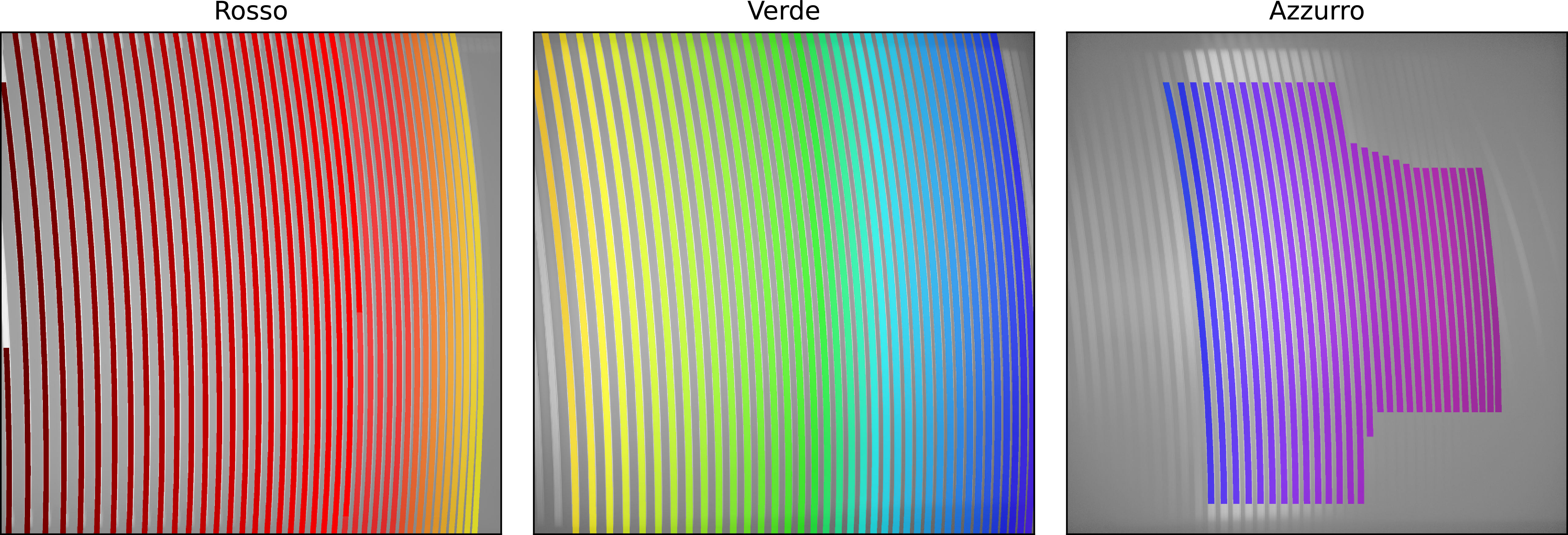
An illustration of the traces for all three Veloce arms from left to right: ‘Rosso’ (red arm, 596–950 nm), ‘Verde’ (green arm, 442–596 nm) and ‘Azzuro’ (blue arm, 366–442 nm). The orders are colour-coded by approximate wavelength down to
 $\sim$
366 nm. Lower wavelengths than 396 nm are extractable, but rarely usable in practice.

Figure 1. Long description
Panel A: Rosso (red arm, 596950 nm) shows color-coded traces with red and orange hues. Panel B: Verde (green arm, 442596 nm) displays traces with a spectrum ranging from blue to green. Panel C: Azzurro (blue arm, 366442 nm) features traces in purple and blue shades.
The reduction workflow consists of the following steps:
-
1. Load and verify configuration file;
-
2. Identify data files either by reading log file or scanning directory;
-
3. Load list of science targets to be reduced;
-
4. Load traces;
-
5. [Optional] Compute master flat;
-
6. [Optional] Verify trace position and make correction if necessary;
-
7. Depending on wavelength calibration scheme:
static - load solution,
ThAr - build solution,
Laser Comb - load reference;
-
8. Extract science data:
-
(a) remove bias and merge segments into one image (using overscan),
-
(b) [Optional] divide by master flat,
-
(c) [Optional] remove scattered light,
-
(d) extract spectrum by summing flux in cross-dispersion direction within summing regions around traces,
-
(e) assign wavelengths to pixels (with selected method),
-
(f) save wavelength calibrated 1D spectrum in Flexible Image Transport System (FITS) format,
-
-
9. [Optional] Merge spectral orders into single normalised spectrum
There is an option to extract all 3 arms or only the selected one, see Figure 1 for reference of extracted orders. The data are provided with minimal processing (i.e. no barycentric correction, no normalisation or order merging).
3. Data extraction
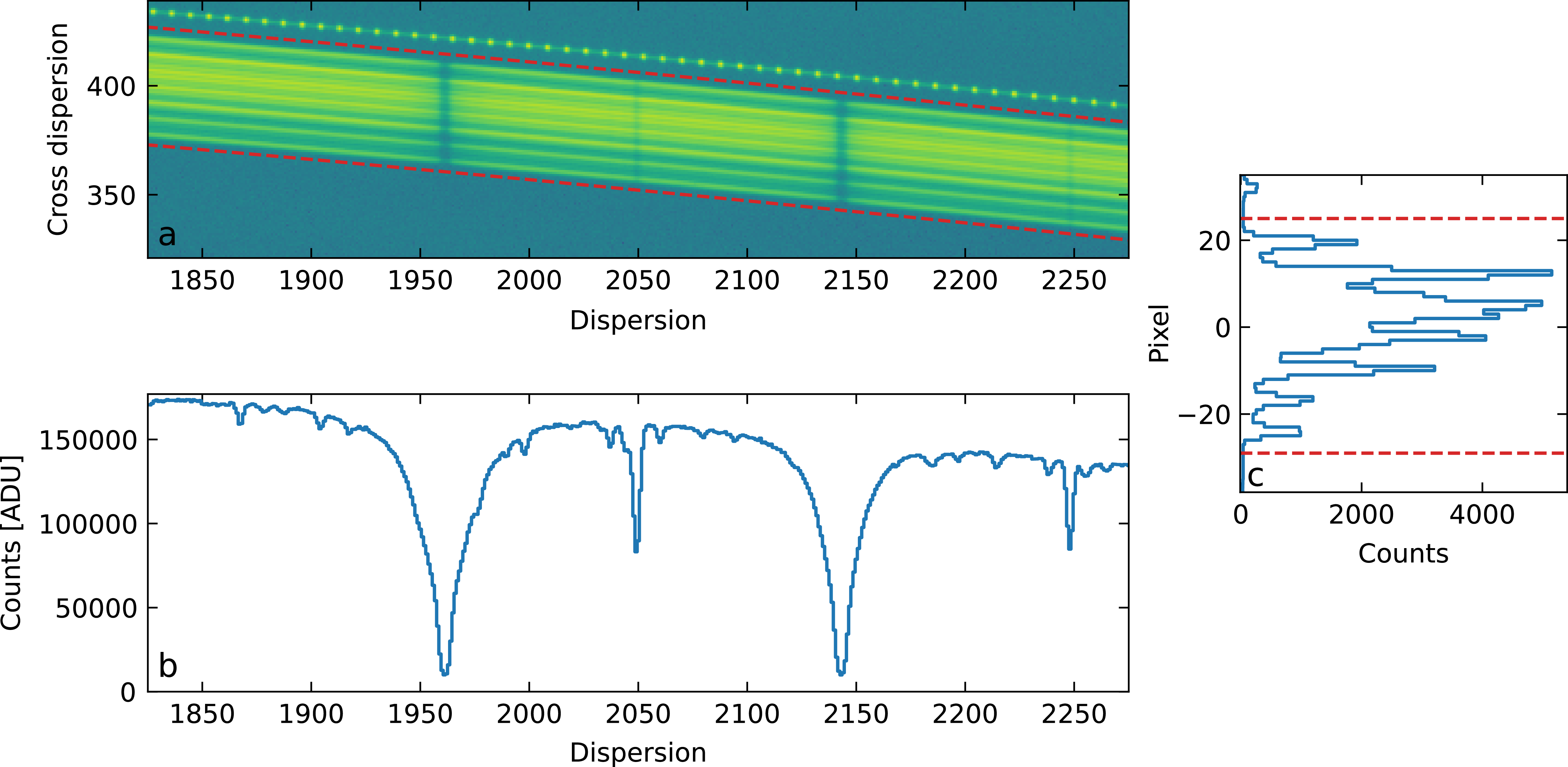
Data extraction is performed by summing up the counts from all pixels in the cross-dispersion direction within a predetermined pixel range (or ‘summing range’) around each trace. The traces are 5th-order polynomials based on simultaneous Thorium traces available from Veloce Manual. The traces are shifted to match the position of fibre flats. Additionally, the summing range was determined by locating the position of blank fibres in the pseudo-slit. To minimise edge effects, we extend the summing range by 2 pixels, see Appendix A for more details on the trace determination procedure. The visual representation of the extraction process is presented in Figure 2.
Demonstration of the extraction. The upper left panel presents a close-up of order 104 in the green arm. The red dashed lines demarcate the summing regions, within which counts are summed in the cross-dispersion direction (columns) to obtain the spectrum in the bottom panel. The right panel shows the cross-section at pixel 2 135 in the dispersion direction. Horizontal red dashed lines mark extent of the summing region. In this example light was not centred on the IFU during the observation which results in asymmetric contribution by different fibres.

Figure 2. Long description
Panel (a) shows a small section of an extracted order on the detector. The horizontal axis is dispersion, and the vertical axis is cross-dispersion. A bright curved band represents the order composed of 19 fibres. Two red dashed lines mark the upper and lower extraction boundaries. Panel (b) shows the one-dimensional spectrum obtained from the extraction. The horizontal axis is the dispersion position (same as panel a), and the vertical axis is counts in ADU. The spectrum contains several spectral lines, including the characteristic sodium doublet. Panel (c) shows a cross-section through the detector image at pixel 2135. The horizontal axis is counts in ADU, and the vertical axis is the pixel position in the cross-dispersion direction. Multiple peaks are visible, corresponding to light from different fibres. Red dashed lines indicate the limits of the extraction region.
The above process is a straightforward approach to the issue of crosstalk between different fibres. It assumes that the fibres are aligned into a perfect pseudo-slit and that the pseudo-slit image is not deformed in the spectrograph. The drawback of this procedure is that (1) the fibres have mutual offsets in the échelle dispersion direction and their point-spread functions overlap on the detector, which is further exacerbated by (2) the pseudo-slit is not perfectly aligned with the detector pixel readout direction. When ignored, this introduces a small broadening that was simulated to be less than
 $\sim$
 $0.2$
km s
 $^{-1}$
in a worst case scenario, see Appendix B.
We confirmed that the magnitude of deformations in the line profiles is negligible in the central region of the detector by examining an observation with excellent conditions (seeing
 $\sim$
1 arcsec, airmass of
 $1.005$
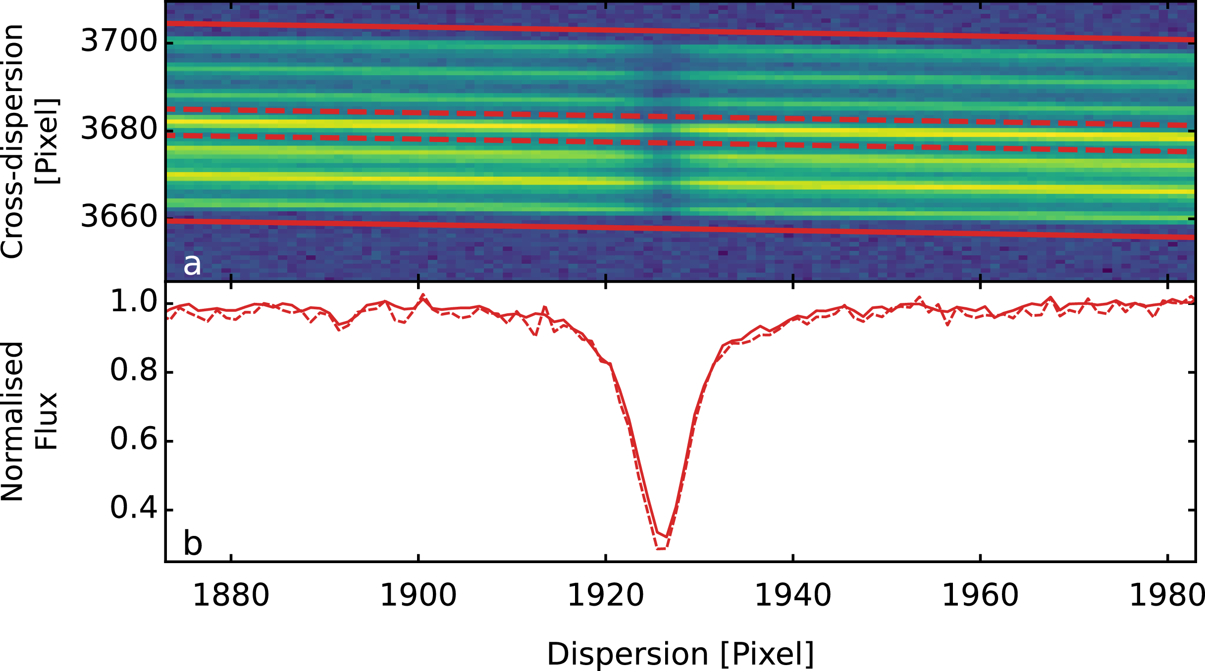
at the start of the exposure). In such conditions, most of the light is concentrated within 7 inner fibres, with minimal contribution from the outer ring, allowing the fibres to be extracted independently. Figure 3 presents a strong isolated line from this observation, demonstrating the difference in line profiles from a single fibre and an entire pseudo slit.
An observation of the G star HD 194640 in excellent conditions. The upper panel presents a small portion of order 100, in the red arm, that contains a Ca I line at 612.2 nm. The seven almost-horizontal lighter streaks correspond to light captured by inner fibres with minimal contribution from the outer rings (note that there are two outer ring fibres in between each of seven inner fibres). Red lines represent the boundaries of the summing ranges used to extract the spectrum shown in the lower panel. The solid line shows the extraction of all fibres, while the dashed line shows the extraction of just the central fibre. A comparison of fitted Gaussian profiles for the seven extracted fibres demonstrates a standard deviation of 0.14 pixel in peak position and 0.55 pixel in full width at half maximum.

Figure 3. Long description
Panel A: A heatmap displays spectral data with cross-dispersion in pixels on the vertical axis and dispersion in pixels on the horizontal axis. The heatmap shows multiple horizontal streaks, with red lines indicating the boundaries of summing ranges. Panel B: A line graph shows normalized flux on the vertical axis and dispersion in pixels on the horizontal axis. The solid red line represents the extraction of all fibers, while the dashed red line represents the extraction of just the central fiber. The graph shows a notable dip in normalized flux around the 1920 pixel mark.
This effect will be more important for stars with low projected rotational velocities (
 $v \sin i \lesssim 10$
km s
 $^{-1}$
). However, it is valid when the broadening is negligible with respect to the science goals and/or target properties. Extreme precision radial velocities will be additionally affected by the fibre mutual offsets and the changing flux through those fibres due to variable seeing conditions. Hence, this approach will not deliver adequate radial velocity precision.
The result of the data extraction process is that for each order, there is a 1D array representing fluxes in each 1-pixel bin along the dispersion direction. To obtain a science-ready spectrum, the flux array needs to be wavelength calibrated.
4. Wavelength calibration
Wavelength calibration is an essential part of the data reduction process. Its precision is crucial for final data quality and applicability. There are several approaches to obtaining solutions for wavelength calibration: (1) use simultaneous calibration (Murphy et al. Reference Murphy2007b) (2) interpolate a solution from calibrations before and/or after observation (Lovis & Pepe Reference Lovis and Pepe2007; Murphy et al. Reference Murphy, Tzanavaris, Webb and Lovis2007a), or (3) assign a static solution (not recommended).
The pipeline includes the three aforementioned modes of producing a wavelength solution. It does not implement wavelength calibration using a simultaneous ThXe lamp because the strong Xe lines pose a risk of bleeding light into the science spectrum. The derivation of a wavelength solution from the simultaneous ThXe calibration and the interpolation of the solution obtained from bracketing ThAr or Laser Comb calibrations (taking ThAr calibrations before and after each target observation), are left as future extensions to the pipeline. That means that pipeline includes: the laser comb for simultaneous calibration (1), calibration with ThAr arc lamp from the night (2) and a static solution as a fallback (3). With these implemented approaches to wavelength calibration, the pipeline is suitable for all general use cases except precision radial velocity.
4.1 The static wavelength solution
The simplest approach is to assign the wavelength based on a single reference solution. It is a very simplistic approach and should be avoided when possible. It is implemented here as a fallback for the rare case where a wavelength solution could not be obtained from calibrations taken that night, or from other recently obtained data.
As a static solution, we used a master ThAr calibration taken on 28 August 2023 during the community science verification run. The solution was obtained in a process described in Subsection 4.2. To match observed lines with the thorium line list, we used the solution provided by the publicly available Veloce Manual (Tinney Reference Tinney2018), which has been transformed to air wavelengths using the formula used in the Vienna Atomic Line Database (VALD) from Birch & Downs (Reference Birch and Downs1994).
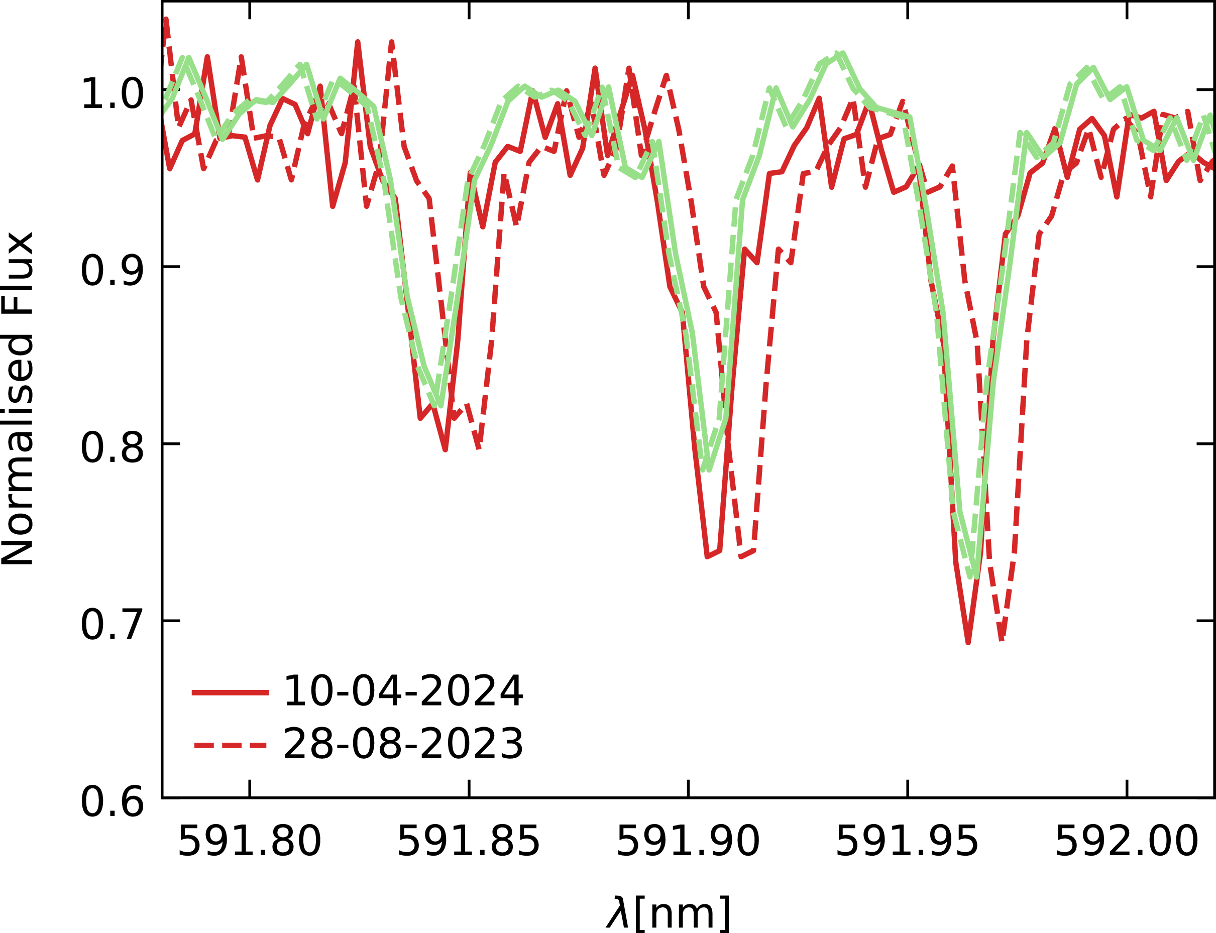
We observed that, even though a Veloce wavelength solution is typically stable within an observing run, some differences can be seen when comparing different runs. These are not only small variations due to changing conditions, but also larger shifts caused by technicians working on the spectrograph. The changes to the wavelength solution can include offsets between different arms, as seen in Figure 4, which highlights differences in line positions between the red and green arms. It is standard practice to perform wavelength calibration each night, even if precise radial velocity is not required. Considering the mentioned phenomenon, special care is required when transferring the solution between different observing runs, and calibrating with the ThAr arc lamp or simultaneous Laser Comb is strongly recommended.
The region of overlap between the green and red arms, marked in green and red accordingly. Dashed lines represent the wavelength solution from another run applied directly, while solid lines represent the calibration obtained from an ThAr arc lamp on the same night, highlighting a much better match.

4.2 Absolute calibration with ThAr arc lamp
The ThAr arc lamp calibrations are an excellent source of the absolute wavelength reference. Observers following the Veloce User Manual (Tinney Reference Tinney2018) will have ThAr calibration blocks at the start and end of the night. Our reduction pipeline computes a median master calibration from consecutive ThAr arc lamp calibrations. The ThAr spectrum is extracted as usual (see Section 3). Then, we match a set of lines observed in the spectrum to those from a prepared Th line list obtained from the National Institute of Standards and Technology (NIST) (Kramida et al. Reference Kramida2024) database. We identify each line that passes a relative intensity threshold for its arm by locating peaks near the expected position of the line, using the in-air wavelength. To find the exact position in pixels along the dispersion direction, we fit a generalised Gaussian (Equation 1) to each line. We discard lines that contain too few points to fit the peak (minimum of 1 point per parameter), that are too weak (line intensity
 $\lt$
1 in background normalised spectrum), or that don’t pass the symmetry criterion which is defined as a ratio of absolute difference between intensity at the line base and the line peak. A line is decided to likely be a blend if this ratio is 0.5, 0.4 and 0.3 for red, green and blue arm, respectively.
 \begin{equation} f(x) = A\exp\left[-\left( \frac{x-\mu}{\sqrt{2}\sigma}\right)^\beta \right]\end{equation}
where A is the amplitude, x is the variable (pixels in this case),
 $\mu$
is the location,
 $\sigma$
is the width, and
 $\beta$
is the shape parameter (when
 $\beta = 2$
is Gaussian). To fit the lines we used curve_fit procedure from scipy package (Virtanen et al. Reference Virtanen2020), using five free parameters: A,
 $\mu$
,
 $\sigma$
,
 $\beta$
and a baseline level. The coordinates of the highest peak around the expected line position are the initial guesses for amplitude and
 $\mu$
. Both initial
 $\sigma$
and
 $\beta$
are set to 2 px, and the baseline is set to the local minimum around the expected line position. Very broad boundary condition are set to
 $0.8$
–
 $2.5$
times the initial amplitude,
 $\mu$
within 3 px of initial position,
 $\sigma$
and
 $\beta$
:
 $10^{-3}$
–5, baseline 0–
 $0.5$
of initial amplitude.
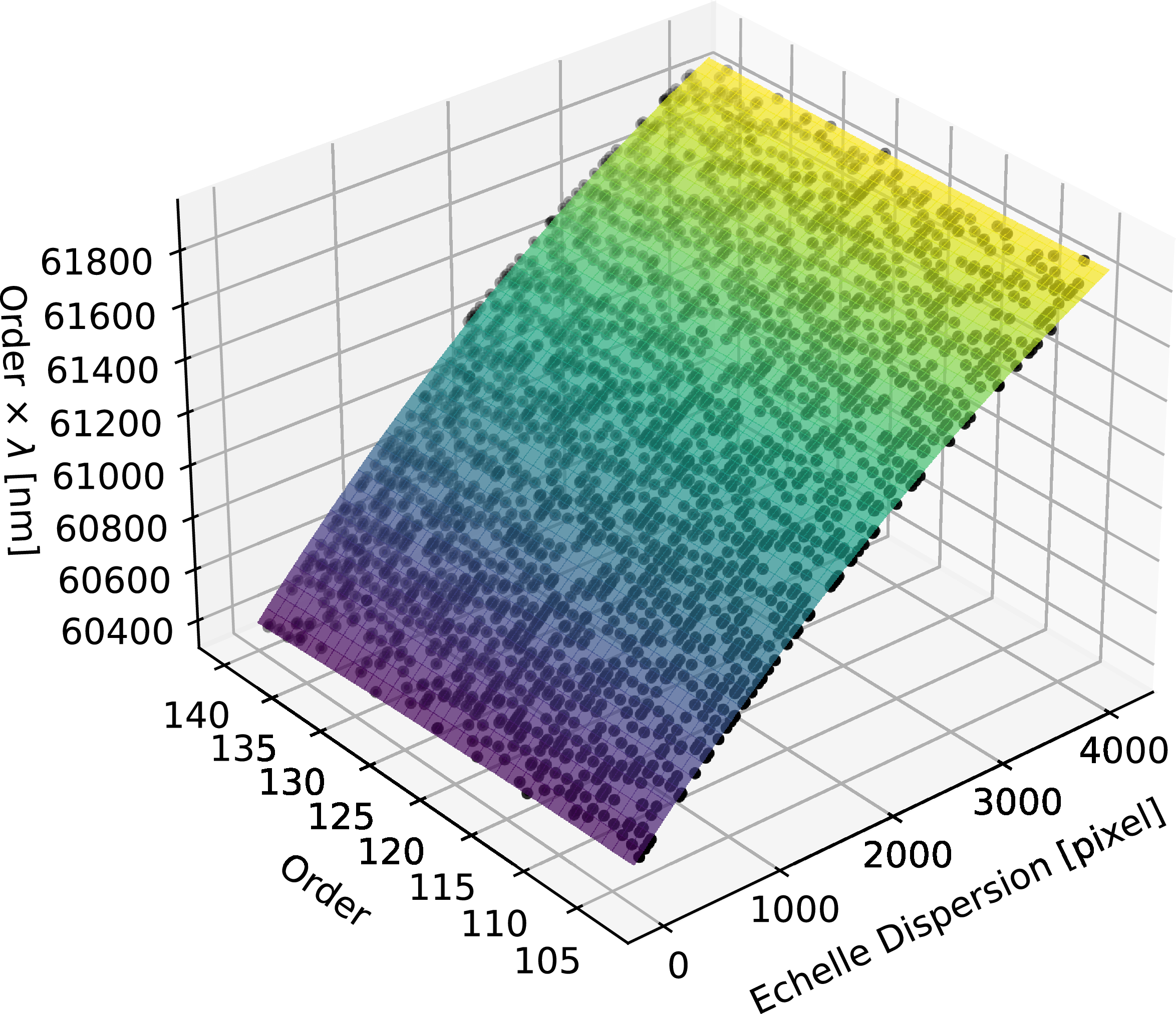
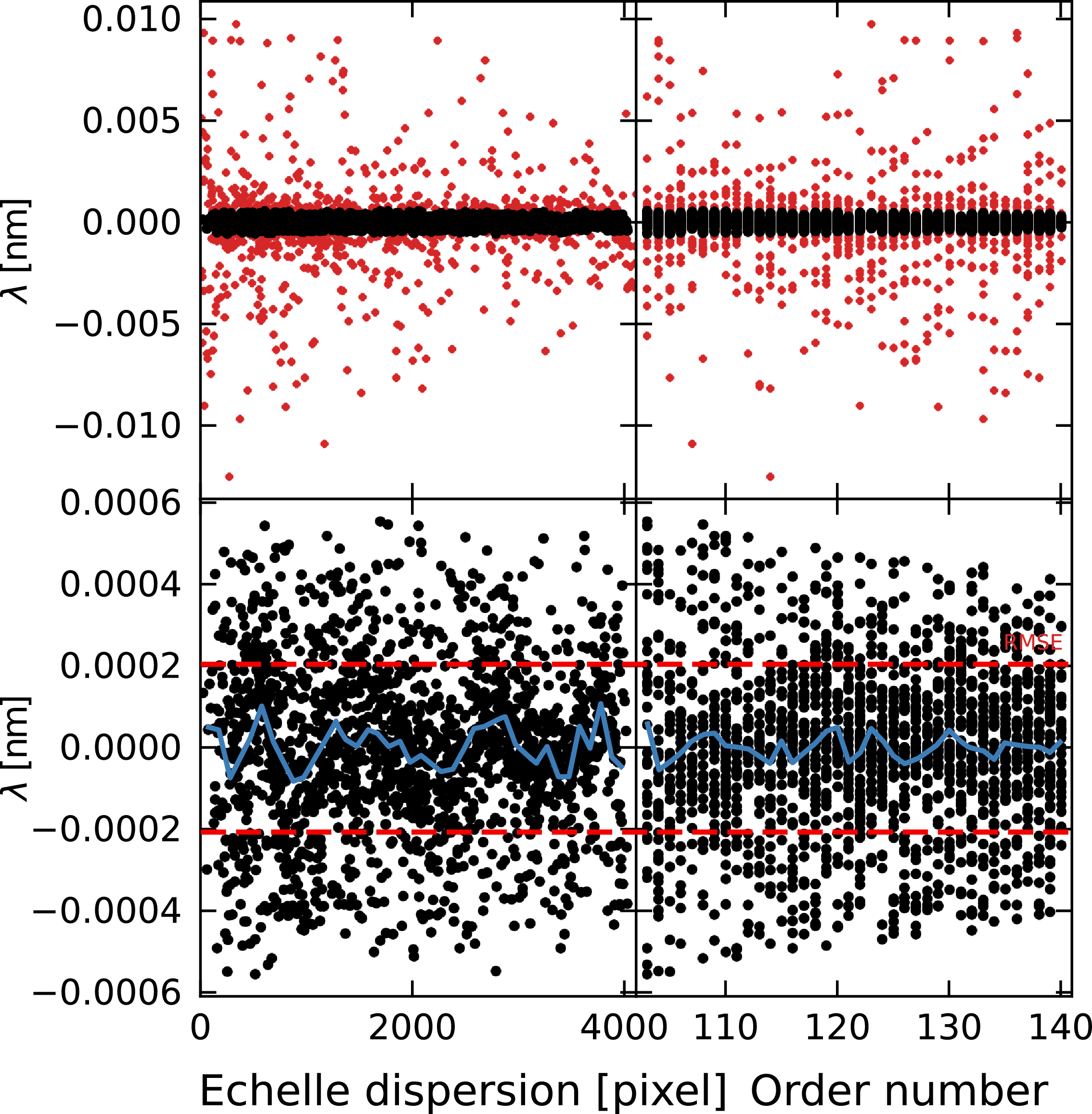
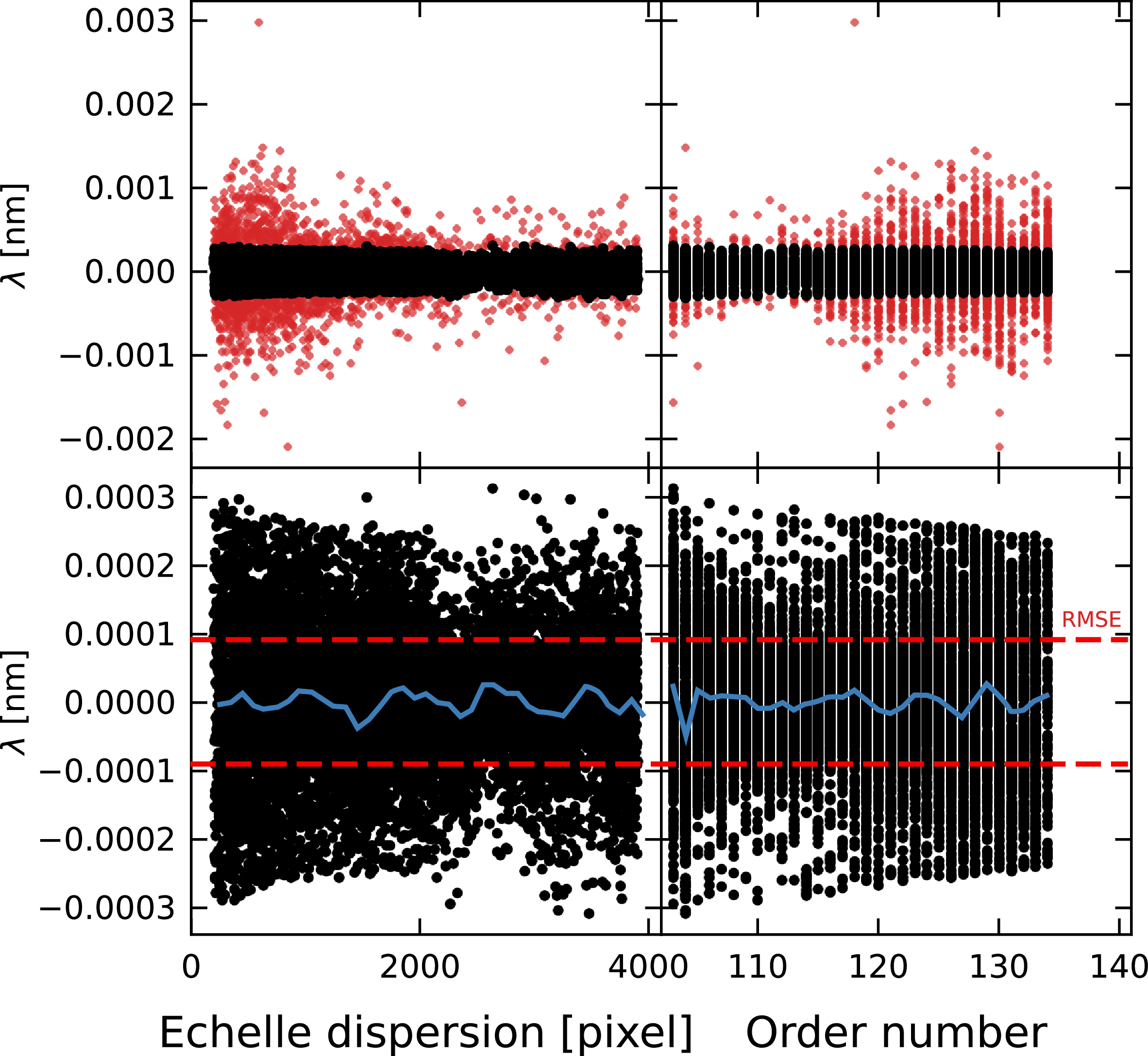
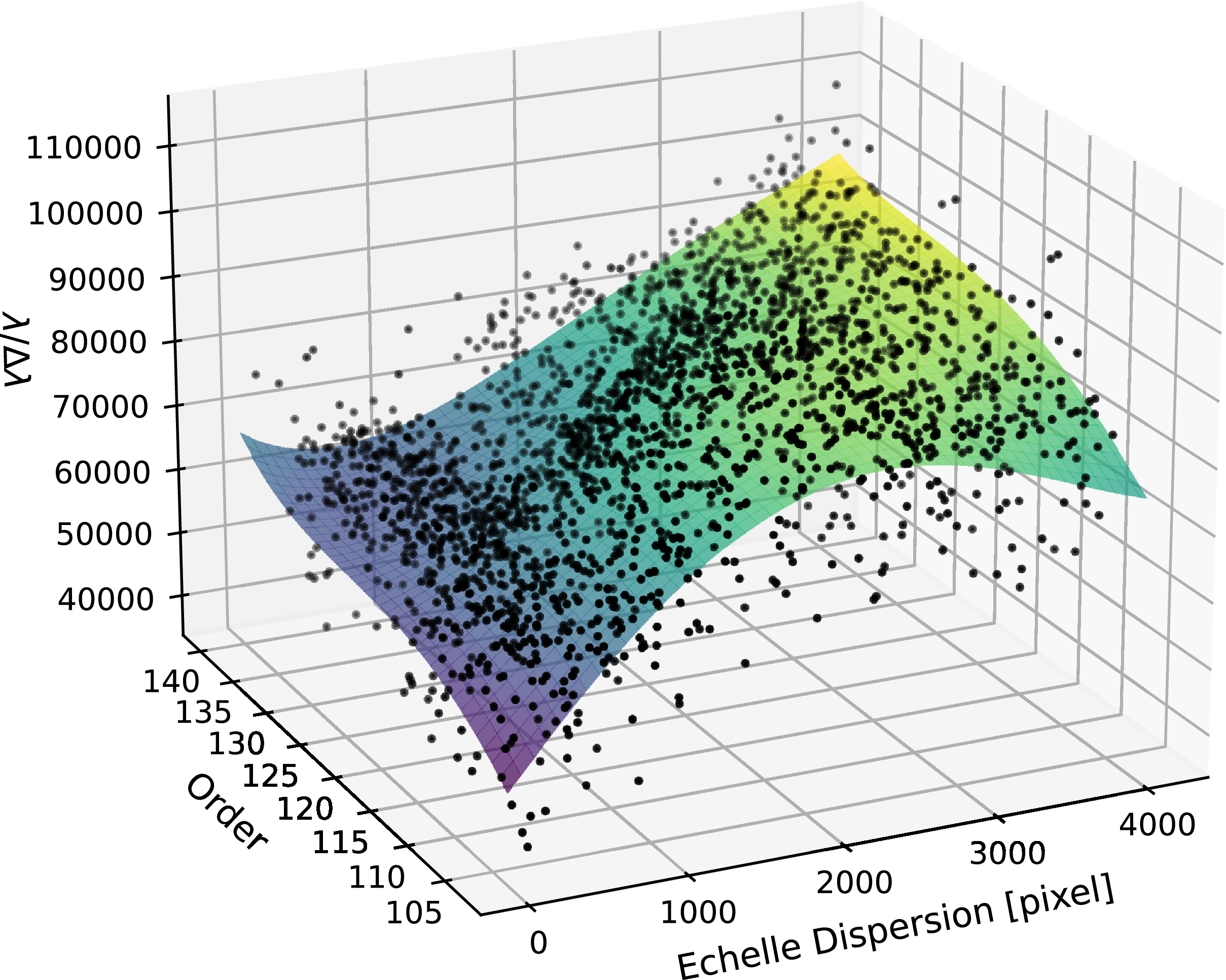
Subsequently, we fit a two-dimensional polynomial surface (7-by-7 degree polynomial for the red and green spectral arms, or 6-by-6 degree polynomial for the blue arm) to a data cube comprising pixel positions, absolute order numbers, and air wavelengths scaled by order number; as seen in Figure 5. We applied iterative outlier rejection via sigma-clipping of residuals. Polynomial degree and sigma clipping level were determined per arm using a grid search that minimised root-mean-square error (RMSE) in velocity and maximised the number of lines used for solution. To provide diagnostic information on the quality of the solution, the pipeline outputs a diagram of the position of lines and the fitted surface, and more importantly, the residuals of the wavelength solution; the residuals for the green arm are shown in Figure 6, and residuals for other arms behave in a similar way dropping towards blue orders.
Surface representing a wavelength solution from the ThAr arc lamp on 28 August 2023. It is a
 $7\times 7$
degree polynomial fitted to air wavelengths of reference thorium lines multiplied by order number. Black points represent line positions in this 3D data cube showing a good coverage on the detector.

Figure 5. Long description
A 3D scatter plot representing a wavelength solution from a ThAr arc lamp on 28 August 2023. The plot shows a surface fitted to air wavelengths of reference thorium lines multiplied by order number. The horizontal axis represents the order, ranging from 105 to 140. The vertical axis represents the order multiplied by wavelength in nanometers, ranging from 60400 to 61800. The depth axis represents the echelle dispersion in pixels, ranging from 0 to 4000. Black points represent line positions in this 3D data cube, showing good coverage on the detector. The points form a surface that is fitted with a degree polynomial, indicating a well-defined relationship between the order, wavelength, and dispersion.
The residuals of a wavelength solution for the green arm from the ThAr arc lamp on 28 August 2023. The red points in the upper panels represent the residuals of lines discarded through sigma clipping; only the black points are included in the fit, and only these are shown in the lower panels. There, dashed red lines indicate the root-mean-square error of the fit. The left-hand side panels are expressed as a function of échelle dispersion, with the binned mean plotted in blue. The right-hand side panels are expressed as a function of échelle order, with the blue line representing the per-order mean.

Figure 6. Long description
Four-panel residual plot with black and red points. Wavelength residuals versus échelle dispersion (left) and order number (right). Trend lines are displayed in blue, and root-mean-square error is plotted as red dashed lines at +/- 0.0002 nm.
4.3 Simultaneous Laser Comb
The Laser Comb can be used to get a wavelength solution that has much better coverage of the dispersion coordinate. It is simultaneous to the scientific exposure, granting robustness against changing conditions.
As per the Veloce Manual, the wavelengths of peaks in the Laser Comb spectrum are determined by the following (Equation 2):
 \begin{equation} f_n = n \times f_{r} + f_\mathrm{0}\end{equation}
with
 $f_n$
representing the wavelength of n-th peak,
 $f_r$
the repetition rate equal to 25.00000000 GHz. and
 $f_0$
the offset frequency equal to 9.56000000000 GHz. These very precise reference values should be constant, however the pipeline will check the FITS header for agreement. In the case of different values, a new wavelength solution must be built. We prepared two approaches for obtaining wavelength solutions from the simultaneous Laser Comb: fitting individual peaks of the Laser Comb (Section 4.3.1), and cross-correlating them with a reference solution (Section 4.3.2).
4.3.1 Building new Laser Comb solution
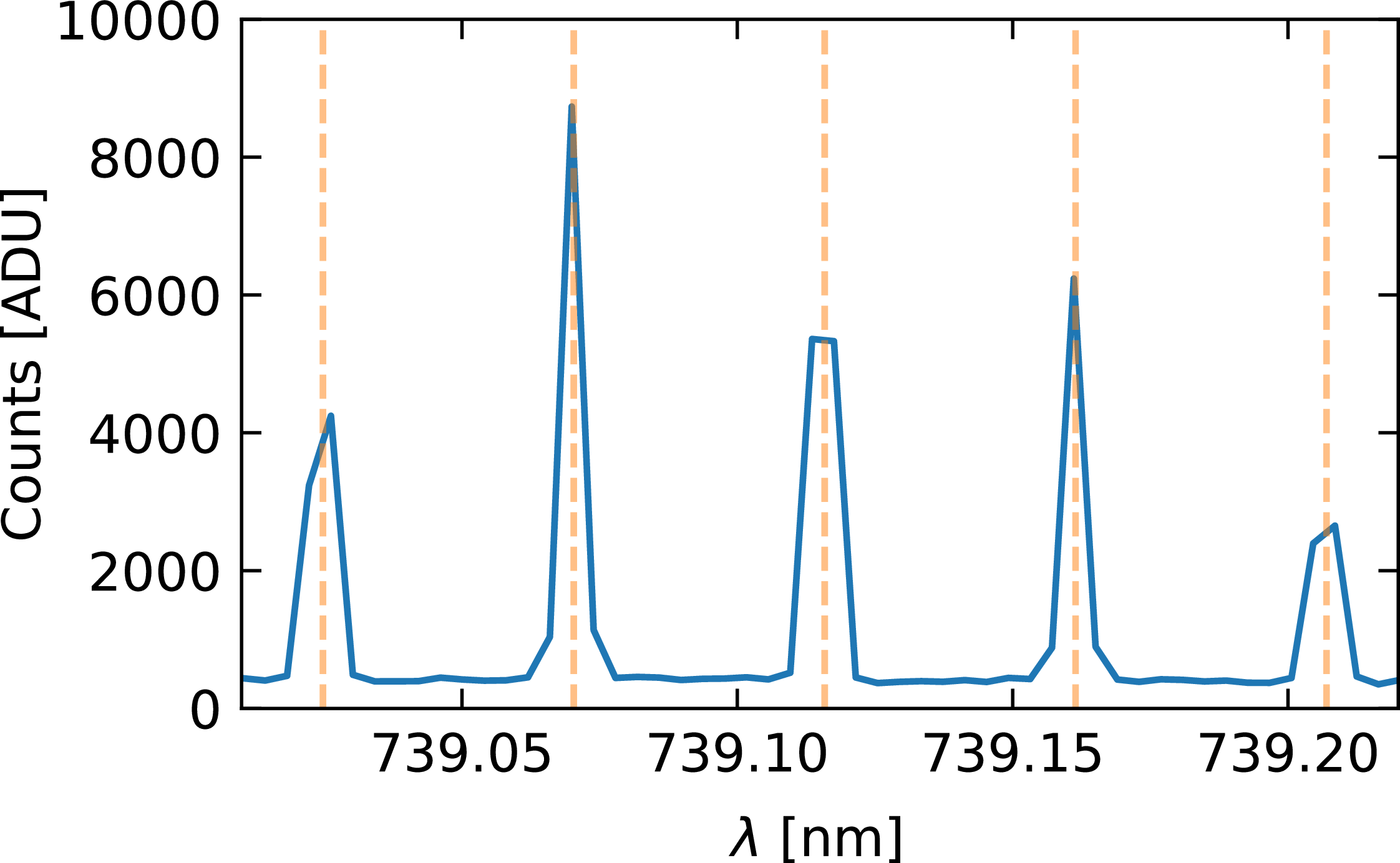
Building a new Laser Comb solution resembles the process of calibration with the ThAr lamp. First an initial wavelength solution is required, preferably from the same night and using in-vacuum wavelengths. Instead of a sparse thorium line list, the positions of the Laser Comb lines are determined with (Equation 2), typically the initial guess should land close to the line peaks, as in Figure 7. Then, peaks are fitted with Gaussians (as in Equation 1 with
 $\beta$
fixed as 2) to determine pixel positions in the dispersion direction.
Small segment of one extracted Laser Comb exposure. Wavelength,
 $\lambda$
, is calibrated with thorium lines measured on the same night. Vertical dashed lines represent positions of Laser Comb lines from (Equation 2). It is already a close match. note also the small number of pixel that define each peak.

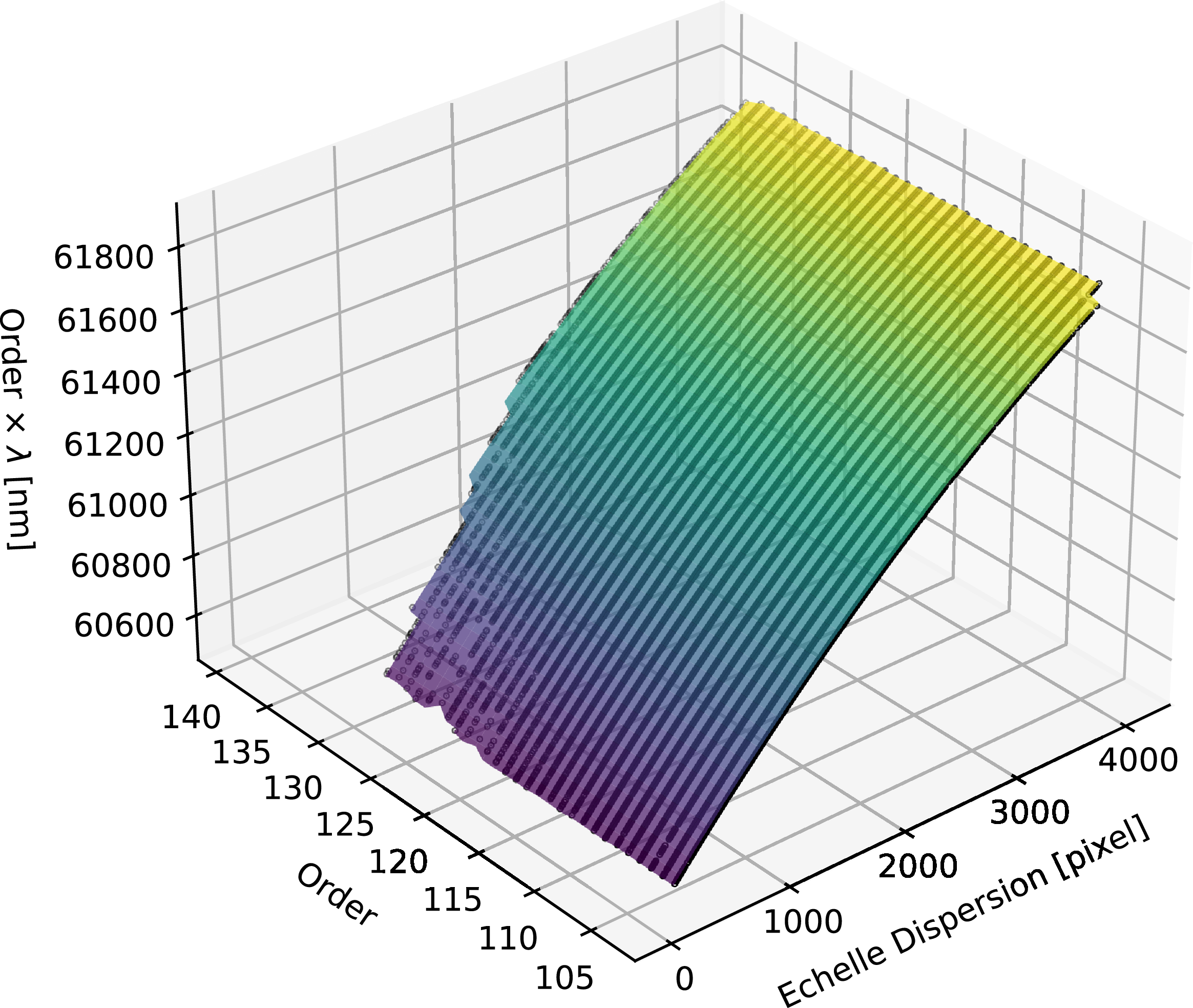
Then a polynomial surface is fitted in the same manner as for the thorium lines, with the difference that the coverage is much more complete in the dispersion direction, but only down to 450 nm in green, since that is the limit of Laser Comb coverage. Typically, line intensities are high enough to cover all orders of the red arm, with slight incompleteness of orders towards shorter wavelengths, most notably in order 104, which, however, is fully covered in the green arm. The coverage is more of an issue in the green arm, where bluest orders are incomplete or sometimes missing entirely. In the final solution, by default when using Laser Comb we include only orders with at least 50 data points and trim orders to regions covered with successfully fitted lines as presented in Figure 8. We allow user to choose to extrapolate the solution; however, caution is advised. Laser Comb calibration is never available for the blue arm. Figure 9 presents the residuals of wavelength solution obtained for the green arm.
As Figure 5, except that the wavelength solution was built by fitting peak positions of Frequency Laser Comb (Section 4.3.1). The solution is confined to cover only the regions of the detector covered by Laser Comb lines.

Figure 8. Long description
A 3D scatter plot representing the relationship between order, echelle dispersion, and wavelength. The horizontal axis represents the order, ranging from 105 to 140. The vertical axis represents the wavelength in nanometers, ranging from 60600 to 61800. The depth axis represents the echelle dispersion in pixels, ranging from 0 to 4000. The data points form a surface that slopes upward from the lower left to the upper right, indicating a positive correlation between the order, echelle dispersion, and wavelength. The surface is color-coded, transitioning from purple at the lower end to yellow at the higher end.
As Figure 6, except that the wavelength solution was built by fitting peak positions of Frequency Laser Comb (Section 4.3.1). There are approximately ten times more lines per order, granting better coverage and the RMSE of a factor of two smaller than for ThAr calibration.

Figure 9. Long description
Four-panel residual plot with black and red points. Wavelength residuals versus échelle dispersion (left) and order number (right). Trend lines are displayed in blue, and root-mean-square error is plotted as red dashed lines at +/- 0.0001 nm.
4.3.2 Cross-correlating Laser Comb
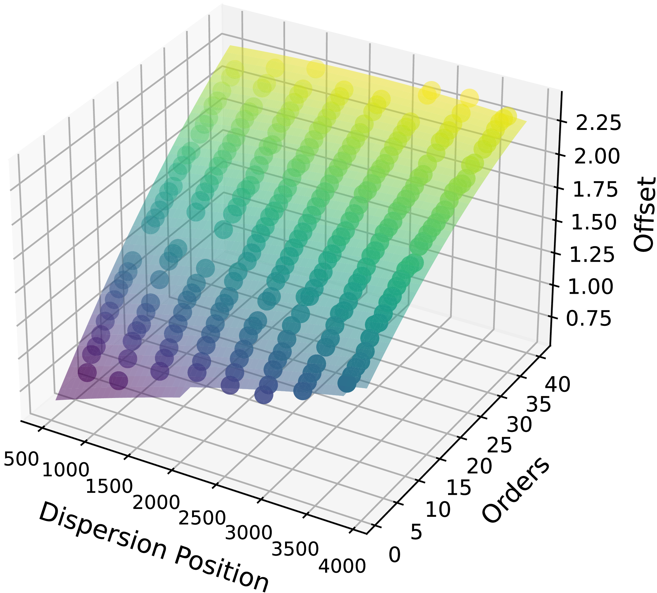
There are thousands of lines in a laser comb solution, which can take some time to compute. In an alternative to fitting and building a new solution for each exposure, we prepared a quick mode for laser comb wavelength calibration. The extracted simultaneous Laser Comb is cross-correlated with a reference solution (defined in Section 4.3.1) to determine the map of adjustments for the reference wavelength solution to match the new observation (Figure 10). We built our reference solution from the frequency Laser Comb exposures taken in the community science verification run in August–September 2023.
Map of offsets between simultaneous Laser Comb calibration and the reference data. Offsets are measured by cross-correlating segments of extracted data. The coordinates of the points are order number and centres of cross correlated regions in dispersion direction expressed in pixels.

Figure 10. Long description
This image is a 3D scatter plot. The x-axis represents the dispersion position in pixels, ranging from 500 to 4000. The y-axis represents the orders, ranging from 0 to 40. The z-axis represents the offset, ranging from 0.75 to 2.25. The plot features a grid with colored spheres indicating data points. The colors transition from purple at the lower end of the offset scale to yellow at the higher end, illustrating a gradient. The data points form a surface that slopes upward from the front left to the back right of the plot, indicating a positive correlation between dispersion position, orders, and offset.
4.3.3 Transferring a Laser Comb solution to science spectra
A simultaneous Laser Comb spectrum is offset in the pseudo-slit from that of the science spectrum (see Figure 2), which means that their wavelength solutions can differ.
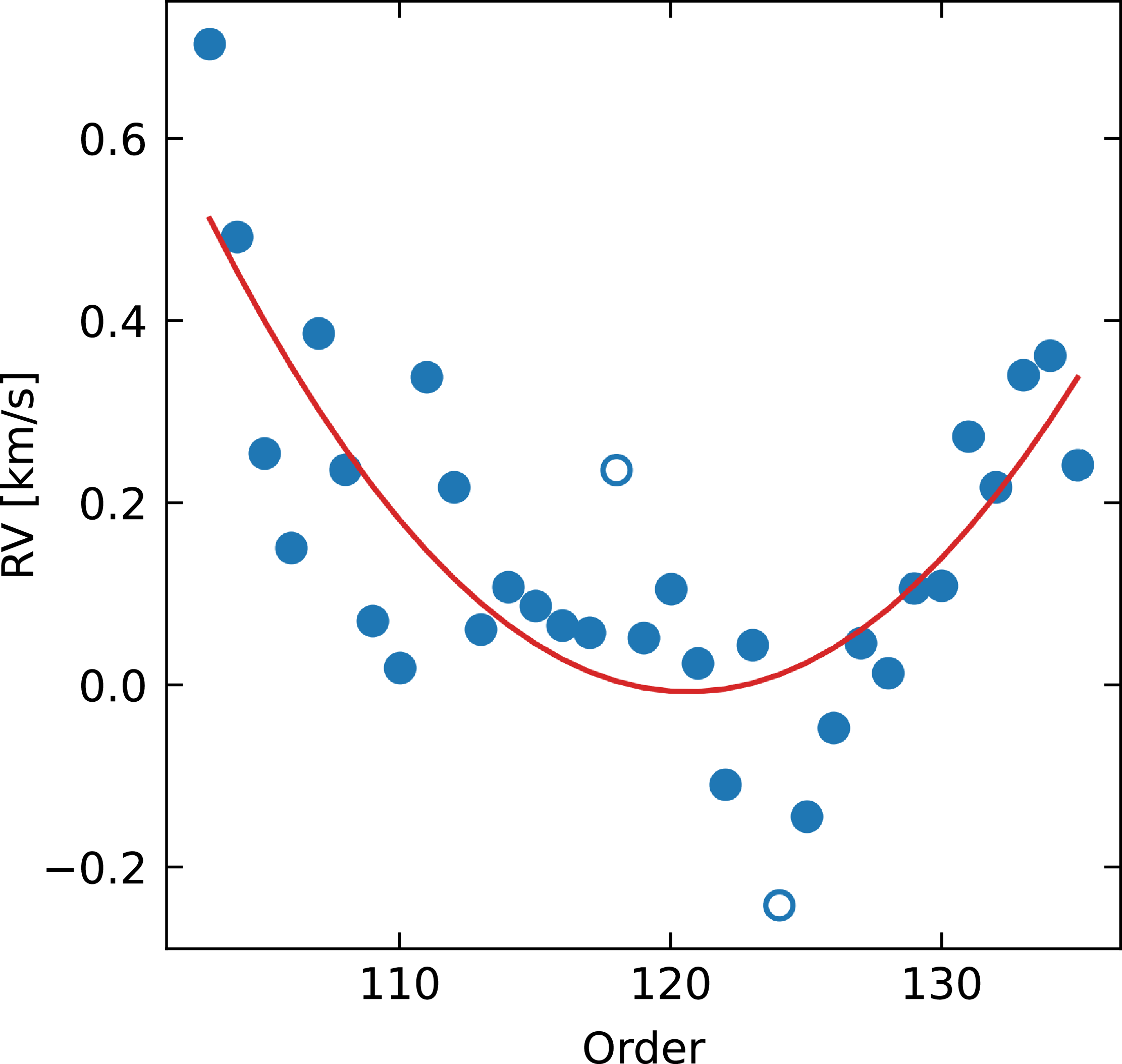
To resolve that issue, for each order, a systematic velocity shift is applied to account for the offset between the calibration and science fibres. The offsets for each order were determined from observations of
 $\tau$
Ceti by cross-correlating its observations with a custom template. The template was generated in iSpec (Blanco-Cuaresma Reference Blanco-Cuaresma2019) using the Synthe radiative transfer code and Atlas9 model atmospheres (Kurucz Reference Kurucz2005), atomic data from the Vienna Atomic Line Database (VALD) (Kupka et al. Reference Kupka and Dubernet2011), and solar abundances from Asplund et al. (Reference Asplund, Grevesse, Sauval and Scott2009). For template computation, we adopted the approximate atmospheric parameters of
 $\tau$
Ceti:
 $T_\mathrm{eff} = 5\,300$
K,
 $\log g = 4.48$
dex,
 $\left[ \mathrm{Fe/H} \right] = -0.55$
dex,
 $\xi = 0.91$
km s
 $^{-1}$
,
 $\zeta = 3.62$
km s
 $^{-1}$
,
 $v\sin i = 0.1$
km s
 $^{-1}$
; where
 $\xi$
is microturbulence and
 $\zeta$
is macroturbulence, estimated using empirical relations implemented in iSpec. Figure 11 presents an example of such offsets for the green arm.
Per order radial velocity offset of the simultaneous laser comb and on sky fibres measured using
 $\tau$
Ceti as a reference.

5. Additional reduction tasks
Data reduction consists of more than just extraction and wavelength calibration. Here we present additional reduction tasks performed during the reduction process, some of which are optional. The tasks, their roles, and the decisions behind their implementation are described in this Section.
5.1 Bias and gain correction
This step is always performed in the reduction process. Veloce detectors measure pre- and post-scan bias for each amplifier in use. Bias correction is performed per exposure by subtracting the median of the overscan regions for each amplifier separately.
In FITS headers, the gain for all quadrants is reported as equal, but it seems they are not. To address discrepancies, we used fibre flats to empirically determine the gain ratio between adjacent quadrants, which we used to scale the quadrants when merging them into a single image before extraction.
5.2 Trace drift
The predetermined trace reflects the position of the light from fibres on the detector. However, small systematic shifts can occur over time, and larger shifts if any intervention of the instrument is carried out. Smaller shifts often negligible, but the scale of larger changes can be significant for the extraction quality (even several pixels).
The most important factor for extraction is the cross-dispersion direction shift, which determines whether the starlight falls fully within the extracted region. The shift is determined by cross-correlating a set of rows of the master-flat exposure with a template distributed with the code. The cross-correlation is performed with the correlate function from numpy package (Harris et al. Reference Harris2020), using mode argument set to ‘full’, then the position corresponding to numpy.argmax is assigned as determined shift for each row. Median of shifts is adopted as the determined drift. We recommend having this option enabled in the configuration; however, it cannot be used for custom defined traces.
The solution seemed stable within a single observing run: cross-correlating fibre flats indicates a
 $\sim$
0-pixel shift, suggesting no need to adjust traces between consecutive nights. The difference before and after the intervention in the cross-dispersion direction can be significant. For example, trace positions for the green arm between 23 May 2024 and 20 June 2024 differ by
 $\sim$
4 pixels (some interventions were performed in between). We haven’t observed a need to completely refit the traces or adjust their vertical position.
5.3 Flat field correction
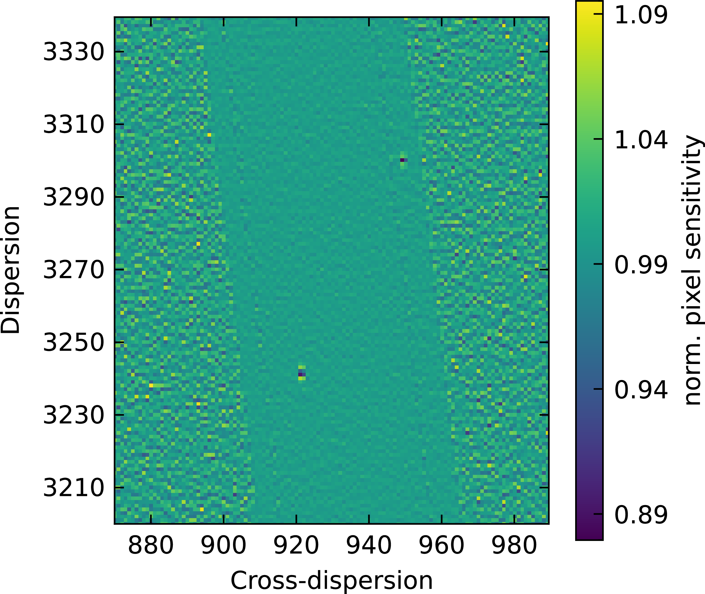
As with any detector, pixels vary in sensitivity. Moreover, it is possible that defects or contaminants are affecting image quality. Fibre flats are the only type of flat-field image included in the standard calibration block for Veloce. We leave flat-fielding as an optional step. We correct for pixel-to-pixel sensitivity differences on the image following the guidelines of Appenzeller (Reference Appenzeller2012) by dividing the science image by a normalised flat. The normalised flat is obtained by smoothing the data in the dispersion direction with a smooth cubic spline (Python implementation of csaps Footnote c with smooth parameter set to 0.5). An example of a region of single order is presented in Figure 12.
An example of a normalised fibre flat used for correcting pixel sensitivity. It is a zoom-in on a small portion of the red arm detector. The broad, darker diagonal stripe running from top-left to bottom-right is the illuminated region corresponding to a single order: science, sky and calibration fibres. The unilluminated regions exhibit higher variance, but this is not a problem because they do not contribute to the extracted spectrum.

5.4 Scattered light
In the fibre flats, there is a significant level of scattered light that we removed for trace determination by fitting the background level between science fibres. Typically, in science exposures, the scattered-light background is very low. In such cases, it is better not to apply this correction because the determination of the background becomes inaccurate. However, for bright targets, it may be an issue, thus, it is left as an optional step disabled by default.
5.5 Flux uncertainty estimate
To provide an estimate of the extracted spectrum flux uncertainty, we assume Poisson stellar noise combined with readout noise. The equation for uncertainty takes the form:
As Figure 5 but vertical axis is resolution. The data points are resolution values estimated from FWHM of fitted thorium lines across the pixel-order position of the green arm. Resolution estimates were fitted with a 4-by-4 degree polynomial.

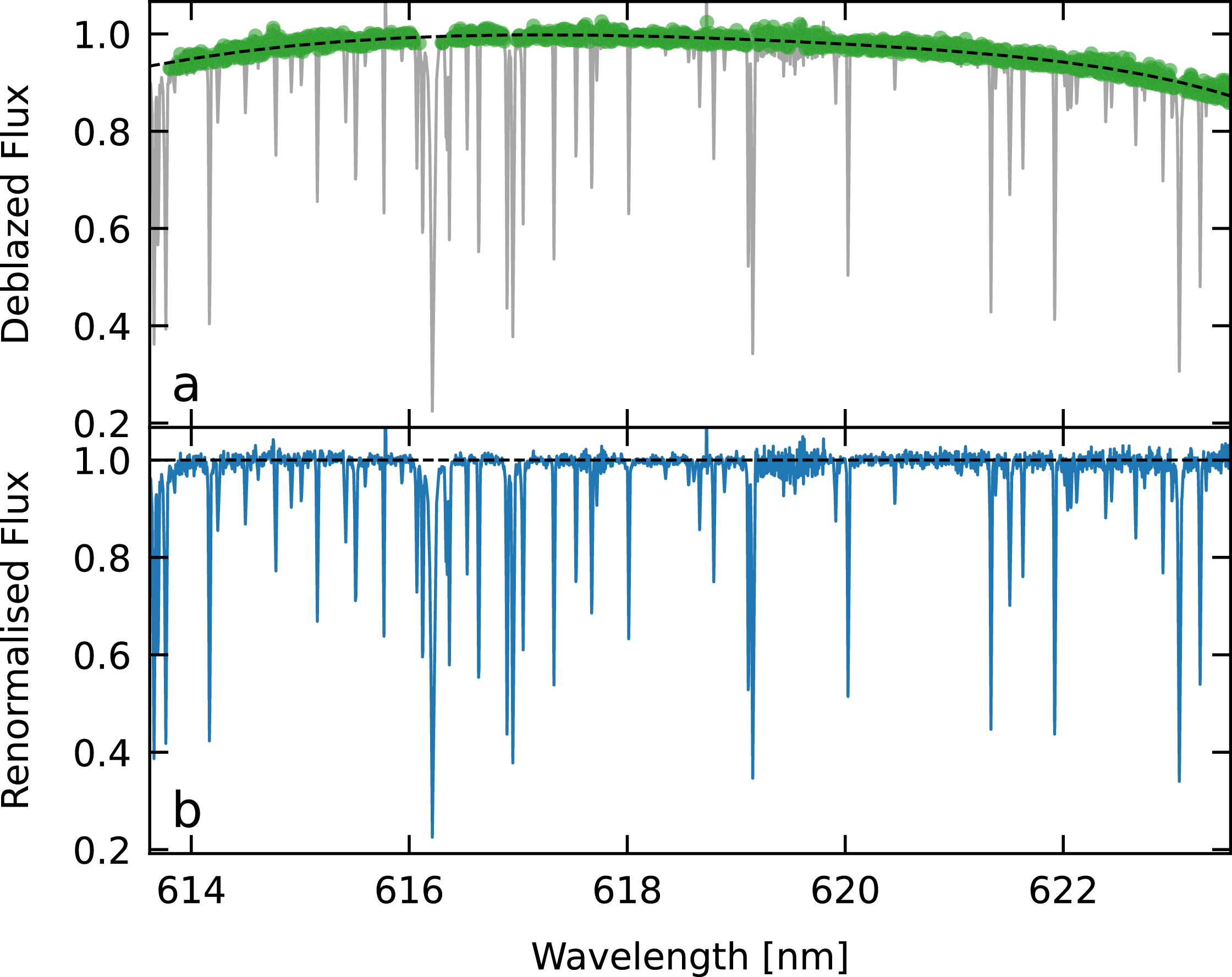
An example of deblazed order renormalisation using
 $\tau$
Ceti observations, performed on order 99 in red arm. In the upper panel, the grey spectrum is the deblazed one, green points mark points used for fitting and the dashed black line is the fitted 4th-degree polynomial. The lower panel shows the renormalised order with a black dashed line marking the continuum.

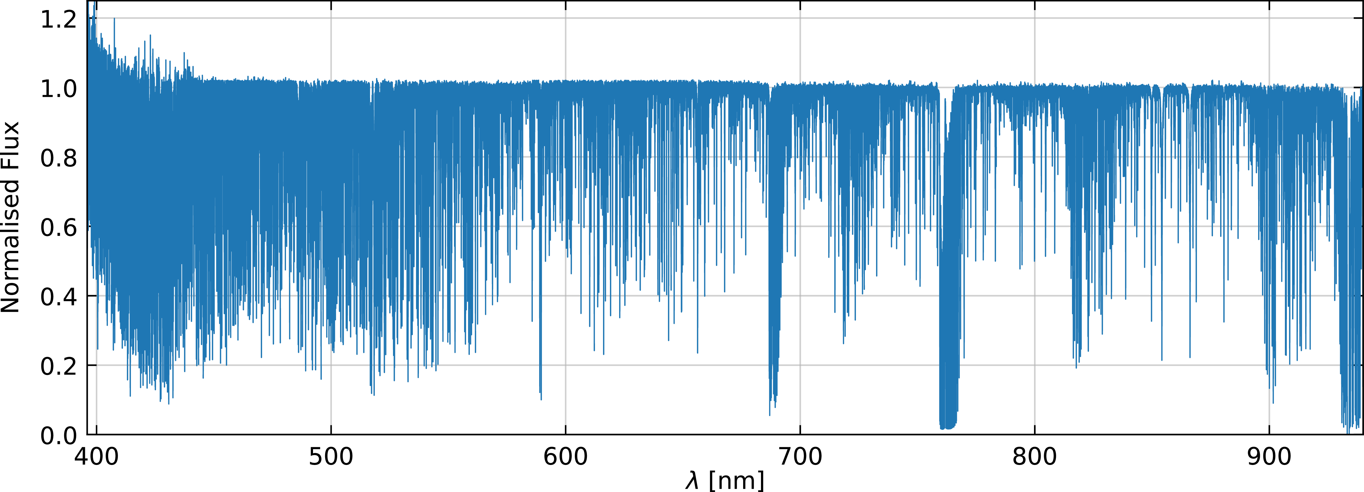
Merged and normalised spectrum of
 $\tau$
Ceti. This spectrum includes the three arms covering the range 396–940 nm. It demonstrates the typical usable spectrum after deblazing and merging.

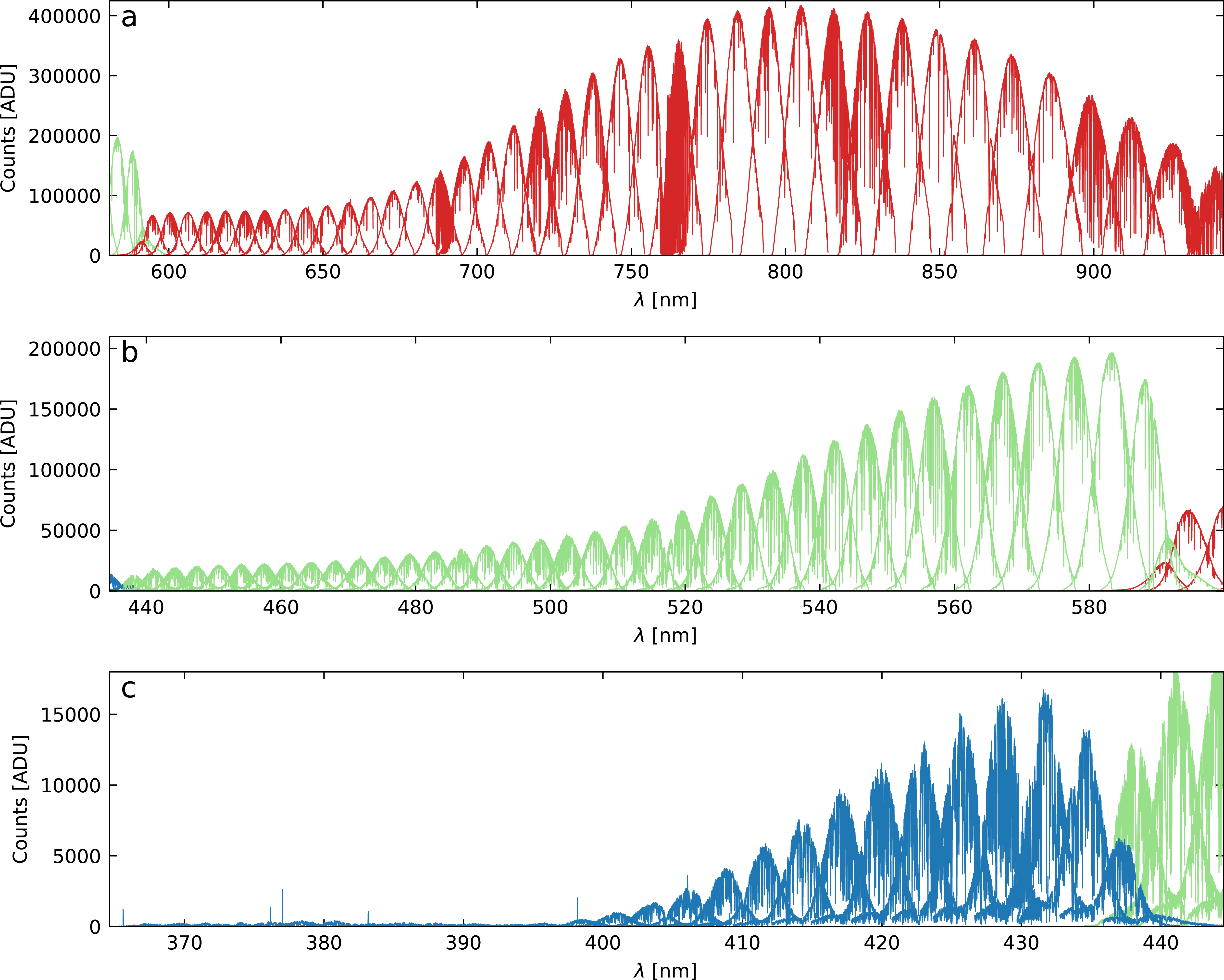
Observation of
 $\tau$
Ceti, showing all extracted orders, panels a, b and c show red, green and blue arms, respectively. Consecutive orders overlap considerably. The overall throughput drops towards the blue wavelengths. The edge orders have lower flux due to the dichroic splitting light into different arms.

Figure 16. Long description
The figure is arranged vertically in three panels labelled A, B and C. All three panels show counts in ADU on the vertical axis and wavelength in nanometers on the horizontal axis. Each panel contains multiple overlapping spectral orders covering adjacent wavelength regions. Consecutive orders overlap by approximately 50%, and several edge orders are repeated in adjacent arms. Panel A shows the red arm. The horizontal axis spans approximately 590 to 940 nm and the vertical axis spans approximately 0 to 400,000 counts. Panel B shows the green arm. The horizontal axis spans approximately 434 to 600 nm and the vertical axis spans approximately 0 to 200,000 counts. Panel C shows the blue arm. The horizontal axis spans approximately 366 to 445 nm and the vertical axis spans approximately 0 to 15,000 counts.
 \begin{equation} \sigma = \sqrt{S_* + n \times N_{\rm read}^2}\end{equation}
where
 $S_*$
is the sum of electrons (
 $e^-$
) from all pixels within extraction region (per pixel in dispersion direction), n is the number of such pixels and
 $N_{\rm read}$
is the readout noise. We assume uniform gain and readout noise for all pixels, as per the instrument specifications (
 $1.01\,\textrm{ADU}/e^-$
and
 $2.5\,e^-$
, respectively). The dark current is remarkably low as per the Veloce Manual (Tinney Reference Tinney2018) and is not included in the current version, but might be added in the future. Similarly, there is no estimation of sky background noise at the time. Flux uncertainty is propagated to the final product by applying the same transformations as to the spectrum itself.
5.6 Resolution
An additional advantage of fitting multiple spectral lines during wavelength calibration using an arc ThAr lamp is the ability to characterise the instrumental profile. Resolution is determined by measuring the full width at half maximum (FWHM) of spectral lines and converting these values to resolution estimates at their respective positions using the equation:
 \begin{equation} R = \frac{\lambda}{\textrm{d}\lambda/\textrm{d}x \times \mathrm{FWHM}}\end{equation}
where R is the resolving power,
 $\lambda$
is the wavelength in nanometers,
 $\textrm{d}\lambda/\textrm{d}x$
represents the dispersion in nanometers per pixel, and FWHM is expressed in pixels. This approach yields a median of approximately
 $75\,000$
from resolution estimates in the green arm. Subsequently, a two-dimensional polynomial is fitted using the same procedure as in wavelength calibration, providing a continuous resolution estimate for each extracted pixel, as shown in Figure 13 and the resolution estimate is an optional output for the pipeline.
5.7 Merging spectral orders
To merge the spectrum, first, the blaze function is determined from the run. The unnormalised master fibre-flats are extracted and smoothed. During the smoothing process, hot pixels and telluric lines in the extracted flats are detected and replaced using linear interpolation. Then the blazes are smoothed with a median filter (51 pixels) and a 1D Gaussian filter (15 pixels) from scipy (Virtanen et al. Reference Virtanen2020).
All science orders are divided by smooth blazes. They are divided by the 95th percentile to place a pseudocontinuum around 1. At this stage, the main deviation of the pseudocontinuum comes mostly from the difference in colour between the flat lamp and the star, it is removed by fitting a 4th-degree polynomial with iterative asymmetric sigma clipping (Figure 14). This was found to improve merging as this process reduces distortions in merged spectra, without renormalisation continuum placement errors have median of around
 $1.8\%$
in 396–930 nm range. By default the last step is not applied to orders that contain strong hydrogen lines or dense telluric absorption to avoid the risk of excessive distortion of these spectral regions.
Then, the fluxes are cleaned by identifying cosmics as peaks with a prominence of at least 3 sigma above the normalised flux, which has been smoothed with a narrow median filter followed by a Gaussian filter. Next, the gaps are filled with linear interpolation.
The merged spectrum is a weighted sum of the normalised flux from all orders. All orders are interpolated onto a common log-linear wavelength grid. The smoothed blazed flux of the observation acts as weights for the orders, interpolated to the same wavelengths. The weights are normalised so that the sum of the weights is equal to 1 at each wavelength step. The resulting spectrum is a single merged spectrum for all available arms, normalised so the continuum is around 1. In some cases, merging can result in large-scale deformations which are not uncommon when merging échelle spectra (Różański et al. Reference Różański, Niemczura, Lemiesz, Posiłek and Różański2022).
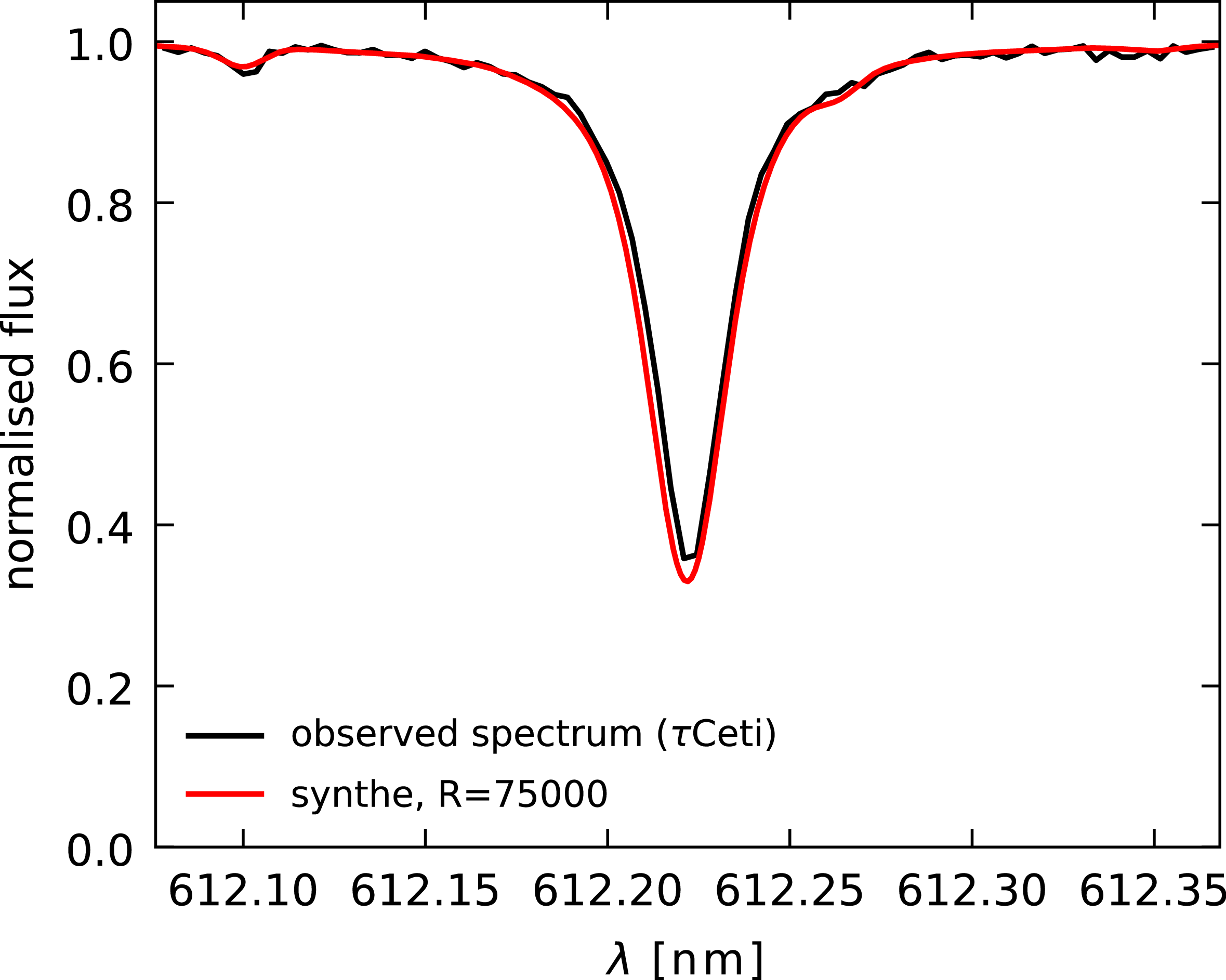
A Ca I line at 612 nm from
 $\tau$
Ceti normalised spectrum compared with a synthetic spectrum computed in iSpec (Blanco-Cuaresma Reference Blanco-Cuaresma2019) with atmospheric parameters of
 $\tau$
Ceti, VALD atomic data (Kupka et al. Reference Kupka and Dubernet2011) and solar abundances from Asplund et al. (Reference Asplund, Grevesse, Sauval and Scott2009), using Synthe radiative transfer code and Atlas9 model atmospheres (Kurucz Reference Kurucz2005); assuming atmospheric parameters of
 $\tau$
Ceti:
 $T_\mathrm{eff} = 5\,300$
K,
 $\log g = 4.48$
dex,
 $\left[ \mathrm{Fe/H} \right] = -0.55$
dex,
 $\xi = 0.91$
km s
 $^{-1}$
,
 $\zeta = 3.62$
km s
 $^{-1}$
,
 $v\sin i = 0.1$
km s
 $^{-1}$
. Synthetic spectrum was broadened to
 $R=75\,000$
, the figure shows that the line profile of reduced spectrum is a close match with theoretical instrumental profile in this case.

6. Discussion
The primary output of the pipeline is a wavelength-calibrated normalised and merged spectrum from all three arms, an example of such a spectrum is presented in Figure 15.
Additionally, three arrays (one for each arm) of wavelength-calibrated fluxes, with wavelengths corresponding to original pixels are supplied. Each row of an array represents an order, and these are not deblazed. Consecutive orders have significant overlap as shown in Figure 16, which shows all orders from the three arms of the spectrograph.
As usual the resolution of produced spectra is approximately limited to the instrumental profile (
 $\sim$
 $4 \,\mathrm{km}\,s^{-1}$
) as shown in Figure 17. However, as described in Section 3, line profiles may be smeared due to a simplistic extraction method. Special attention is required when analysing stars with
 $v \sin i \lt 8.5\,{\rm km}\,{\rm s}^{-1}$
, as the estimated broadening may exceed 1% of the full width at half maximum, yet this is still smaller than the typical uncertainties associated with
 $v \sin i$
measurements for slowly rotating stars.
6.1 Published applications
During its development, the pipeline was used to reduce observations that contributed to published work. Kurtz et al. (Reference Kurtz2025) studied HD 60435, a well-known roAp star that mysteriously stopped pulsating during the 5 yr time-span when it was observed by TESS. Using data from the green arm, a comprehensive determination of
 $v \sin i$
was performed that allowed an estimate of the inclination of its rotational axis to the line of sight, which in turn constrained oblique pulsator models for this enigmatic star. Another example is TIC 88785435, a K dwarf in Upper Centaurus Lupus hosting a super-Neptune (Vach et al. Reference Vach2025). Spectra were used to infer atmospheric parameters of the host star, and measured lithium equivalent widths placed constraints on the age. The latest published work is atmospheric retrieval of WASP-189b (Borsato et al. Reference Borsato2025). The authors performed transmission spectroscopy on a single transit of the ultra-hot Jupiter WASP-189b and detected ionised calcium, among other elements.
6.2 Summary
We present a fully automated pipeline to reduce spectra from all three arms of the Veloce spectrograph mounted on the AAT. It was tested with various targets and modes of observation. It automatically aligns the traces for extraction and keeps them fixed for the run, ensuring consistent analysis of spectroscopic time series. The current version of the pipeline (v1.0.0) uses a simplified extraction that is adequate for most applications, however, it is not suitable for precision radial-velocity work. The pipeline offers three options for wavelength calibration (static, ThAr, and simultaneous Laser Comb). The code is publicly available at GitHub.Footnote d The reduction can be performed by supplying a configuration file and executing a single command. Requests for upgrades can be submitted as GitHub issues or pull requests.
Future development will add more wavelength calibration options such as simultaneous ThXe and ThAr lamp observation bracketing. The pipeline has already been successfully applied in published works.
Acknowledgements
This work is based on observations collected with Veloce spectrograph at the Anglo-Australian Telescope under programs R/2023B/12, A/2023B/05, A/2024B/003, A/2025A/13 and publicly available data from Director time devoted to Veloce Commissioning. We acknowledge the traditional custodians of the land on which the AAT stands, the Gamilaraay people, and pay our respects to their Elders past, present and emerging.
The initial traces and preliminary wavelength solutions are based on those provided in the Veloce Instrument Manual. The authors thank Chris Tinney for these solutions and for the valuable information included in the manual. We also wish to express our gratitude to all individuals who contributed to this resource.
JK was supported by the UniSQ International Stipend and UniSQ International Fees Research Scholarship. SJM was supported by the Australian Research Council through Future Fellowship FT210100485.
Data availability statement
Raw data are available from the AAT archive through AAO DataCentral (archives.datacentral.org.au).
Appendix A. Summing range determination
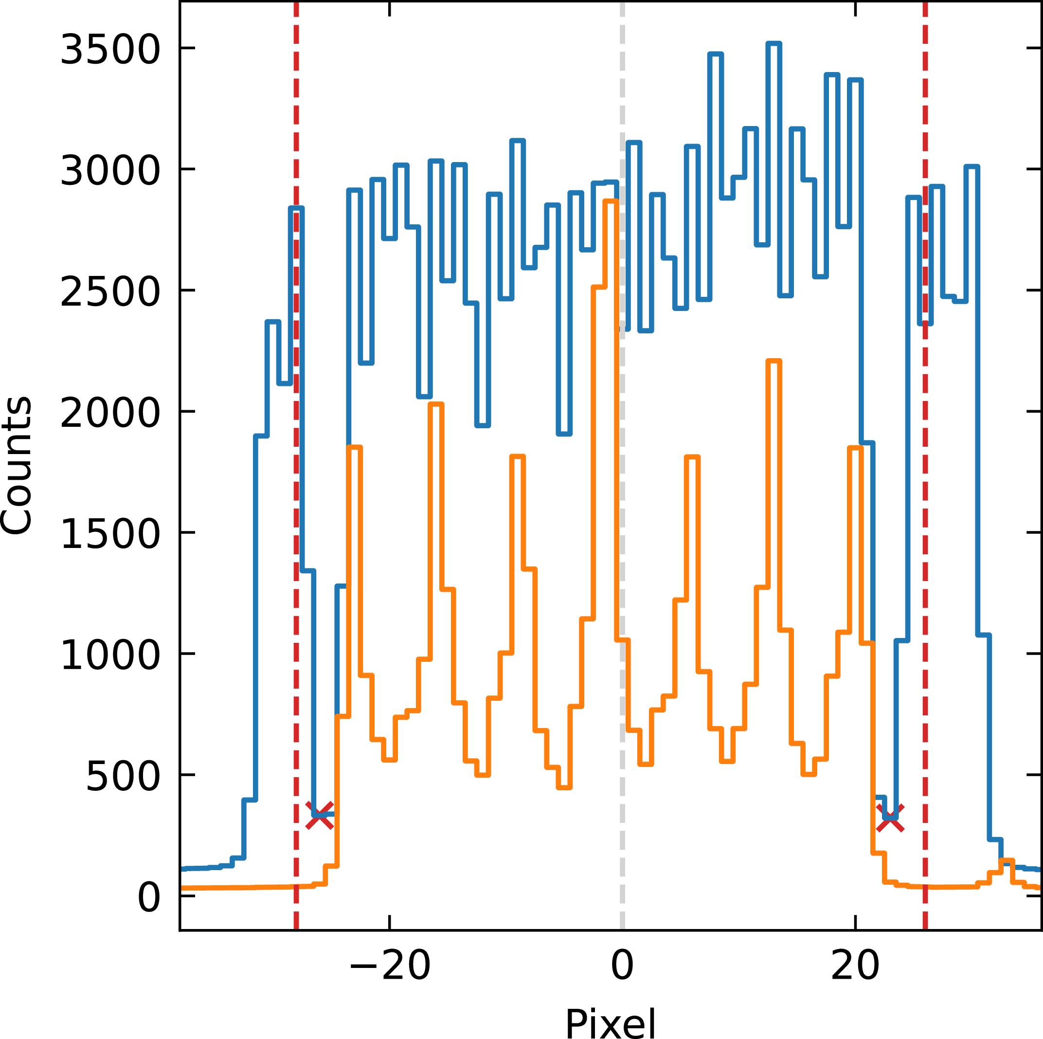
The graph represents cross sections of order 114 in the green arm for a fibre flat image (blue) and a B star HD 136504 (orange). Vertical dashed line represent the position of the trace with horizontal axis being distance from trace in pixels. Low signal caused by the blank fibres are marked with red crosses and adopted extraction limits are represented by vertical red dashed lines.

The traces used in the pipeline are a modification of the simultaneous ThXe traces available in the Veloce Manual (Tinney Reference Tinney2018). We shifted predetermined traces to fit the approximate centre of orders in the fibre flats. Flux-weighted mean positions in the cross-dispersion direction around the preliminary traces were determined, and the traces were refitted to these points. Then comes the crucial step of determining extraction limits: to determine how many pixels around the trace to include. An inspection of the Veloce orders found that they are similar in size and taking 45 pixels on each side of the trace and reshaping the image cutout into a 91-pixel-wide array includes all pixels associated with orders. Then we take the median in the dispersion direction to get an estimate of the cross-section profile of the pseudo slit, as in Figure A1. At first, we set the extraction limits on the blank fibres based on the clear dip in signal between object and sky fibres. These preliminary limits were found too narrow, as stacking multiple consecutive observations revealed low-frequency pattern noise due to edge effects; therefore, we extended the regions by 2 pixels. Finally, for each arm, we adopted the maximum values, so the summing region has the same width at each dispersion step for each order.
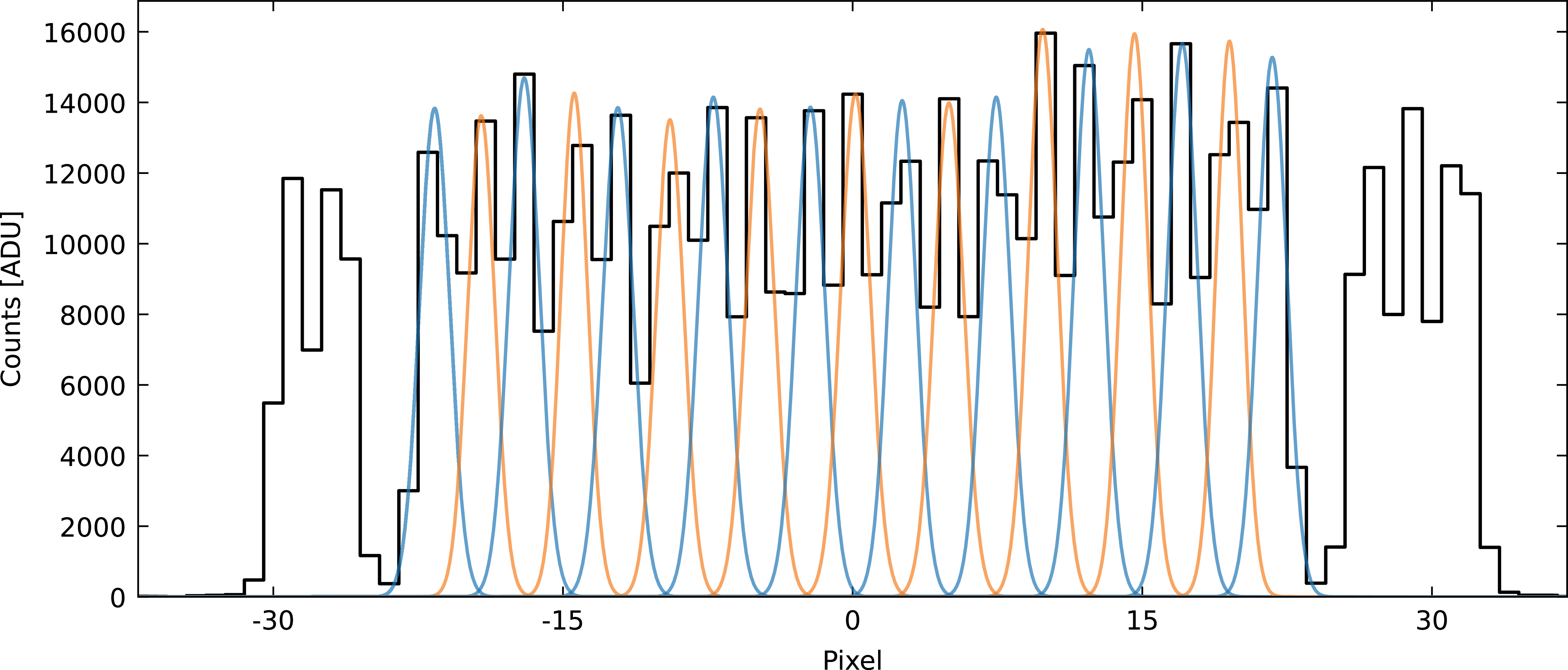
A one-pixel cross-section of a fibre flat exposure in the middle of order 112 in the green arm. In the fibre flat, all fibres are approximately equally illuminated. Alternating blue and orange Gaussian profiles show an estimate of individual fibre images of the 19-fibre science pseudo-slit. Significant overlap of adjacent fibre images is clearly visible.

As a consequence of the above, we kept the original extent of the preliminary order traces from the Veloce Manual. That means, for the blue arm, the traces are not covering full dispersion direction on the detector as presented on the Figure 1, while being clipped consecutive orders in blue overlap providing full wavelength coverage down to
 $\sim$
366 nm, as shown in Figure 16; however, this is typically very low-quality data, and no steps were taken to get the most out of this noise-dominated region.
Appendix B. Examination of broadening due to simplified extraction
Data extraction performed by summing up the counts in the cross-dispersion direction is a commonly used, but imperfect approach. It neglects challenges posed by actual data, such as a complicated slit structure that is not exactly parallel to the échelle dispersion axis. In the case of Veloce, the problem is compounded by a pseudo-slit composed of 19 fibres with mutual offsets and overlapping point spread functions (Figure B1 shows representative overlap of fibres on the fibre flat exposure). We expect the simplified approach to introduce a broadening to the spectral features.
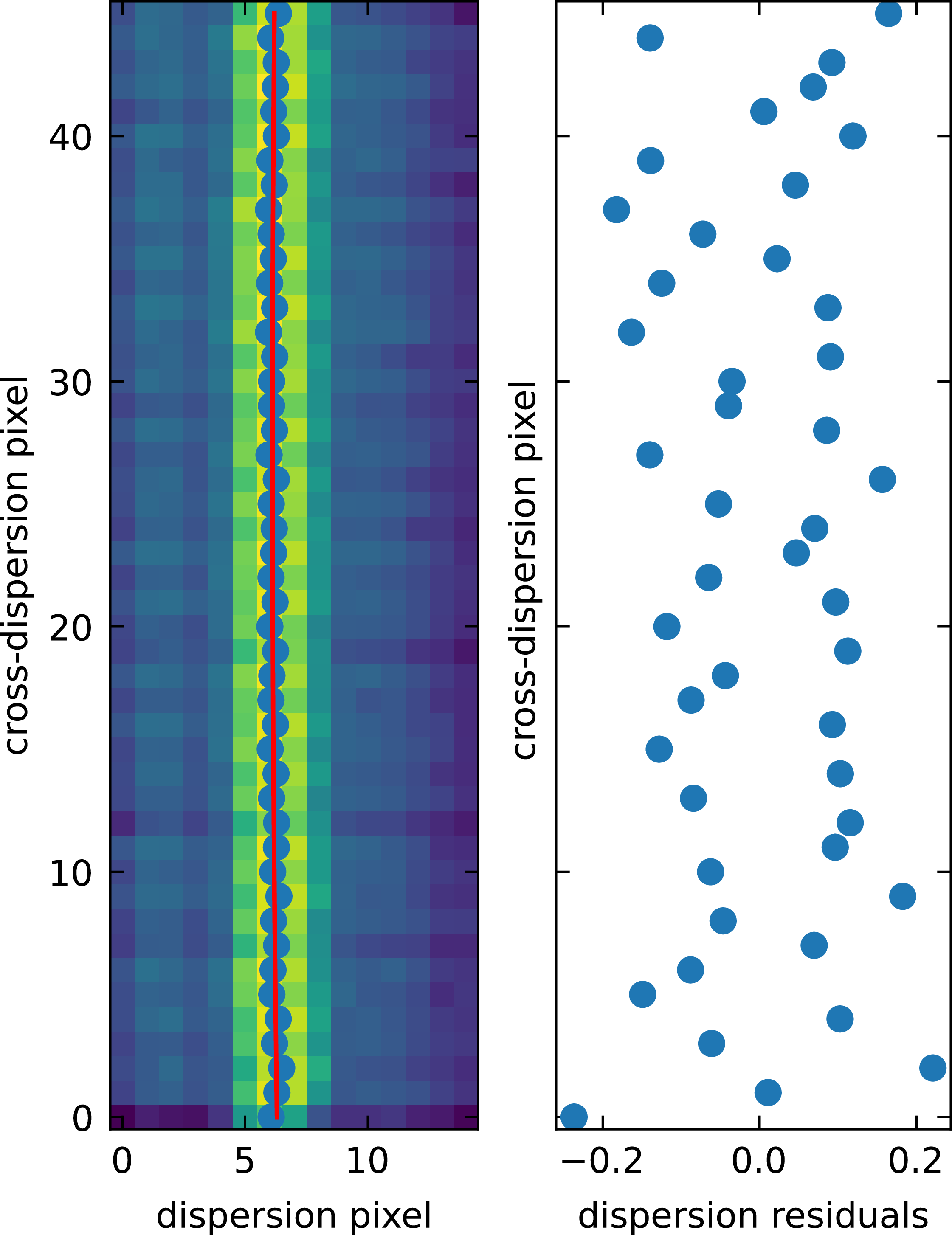
An example of fitting the ‘slit’ offset. Left: the colour map represents counts in ADU, filled blue circles are plotted at the peaks of generalised Gaussians fitted to columns (i.e. along the dispersion direction), and the red line is a 2nd order polynomial fitted to the peak positions as a function of the cross-dispersion direction. Right: the residuals of the fit.

Figure B2. Long description
The left panel has a horizontal axis labelled dispersion pixel and a vertical axis labelled cross-dispersion pixel. A colour map represents counts across the plotted region. Blue filled circular markers are distributed across the image in a curved pattern. A red curve passes through the markers. The right panel has a horizontal axis labelled dispersion residuals and a vertical axis labelled cross-dispersion pixel. Individual points are plotted as a vertical distribution centred near zero on the horizontal axis. The residual values span both positive and negative offsets, mostly within +/- 0.2px.
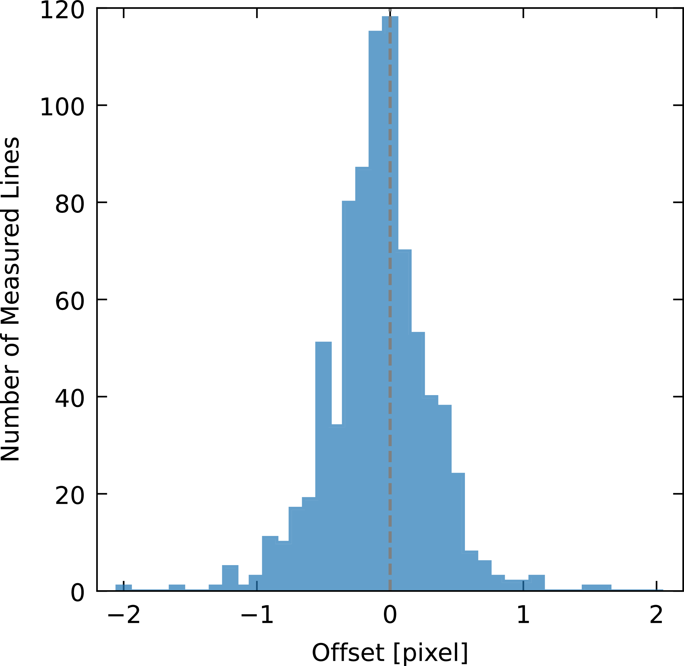
To measure this effect, we investigated fibre arc lamp Thorium-Argon exposures in a procedure inspired by slit tilt and curvature determination (Piskunov et al. Reference Piskunov, Wehrhahn and Marquart2021). Thorium emission lines give sparse signatures of the effective ‘slit’ profile across the detector. Due to the complex profile, we only model the pseudo slit with a second-order polynomial and measure the maximum offsets between fibres. We define these offsets as the difference of the polynomial values at the ends of the pseudo slit in the dispersion direction, measured in pixels. The polynomial is fitted to points obtained as the peaks of generalised Gaussians representing the profile in the dispersion direction (Figure B2). The mean of the determined offsets is -0.09 pixel with a standard deviation of 0.35; however, the distribution is not exactly normal. Figure B3 shows the histogram of offsets for the green arm.
Histogram of measured offsets. The mean lies near (
 $-0.09$
pixel) but not precisely on zero, and the distribution is skewed, i.e. non-Gaussian.

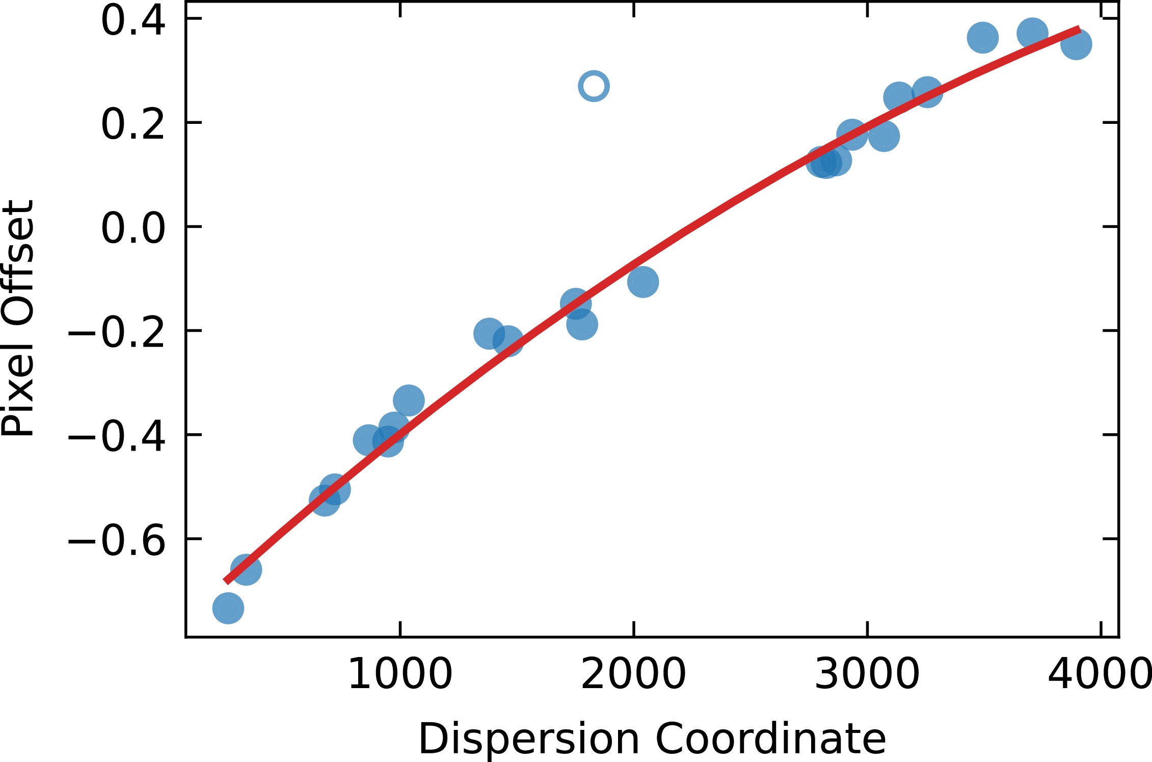
An example fit of offset values as a function of position along the order. There is a clear dependence on the position along the order except the single outlier in this order.

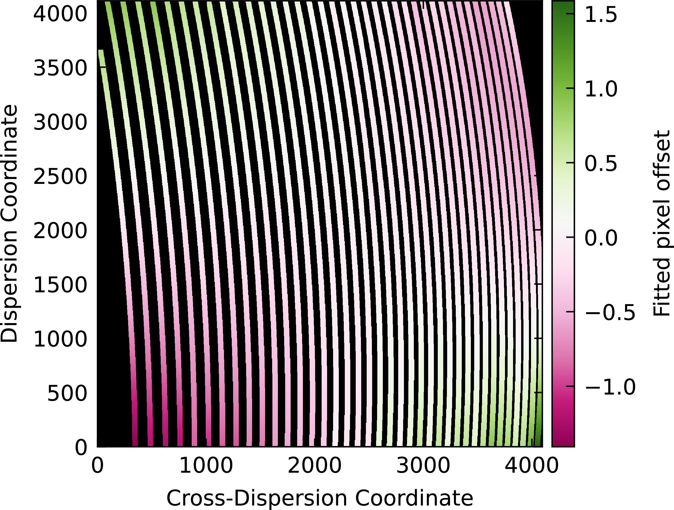
The offset values seem to be a function of the position on the detector. We fitted 2nd-order polynomials to the results of each order, using iterative outlier rejection (e.g. Figure B4). As a result, we obtained the map of offsets, as shown in Figure B5. The map shows that in the central part of the detector, which is most important due to a higher signal-to-noise ratio of spectrum, the offsets are negligible. On the order edges, summing all counts in the cross-dispersion direction in the presence of a non-negligible offset causes additional broadening. Overall, the offsets between the first and last pixel of the ‘slit’ are typically much less than one pixel or
 $\pm$
0.5 px with respect to the centre, which translates to
 $\sim$
2 km s
 $^{-1}$
in the red end of the orders and
 $\sim$
1.4 km s
 $^{-1}$
in the blue. The resolution is degraded by a simplified approach, but not by the exact value expressed in velocity, because it works in conjunction with the physical point spread function of the spectrograph.
Map of determined offsets across the detector, on an order-by-order basis. The colour represents the offset values and, as discussed previously, most values fall within
 $\pm 1$
pixel.

Figure B5. Long description
A heat map represents fitted pixel offsets across a detector. The heat map is structured as a grid with the x-axis labeled as Cross-Dispersion Coordinate and the y-axis labeled as Dispersion Coordinate. The color scale on the right ranges from -1.4 to 1.6, indicating the magnitude of the fitted pixel offset. Lighter colors represent higher offset values, while darker colors represent lower offset values. The heat map shows a gradient pattern with higher offset values concentrated towards the top left and bottom right corners, and lower offset values towards the bottom left and top right corners. The offsets appear to vary systematically across the detector, with distinct regions of higher and lower values.
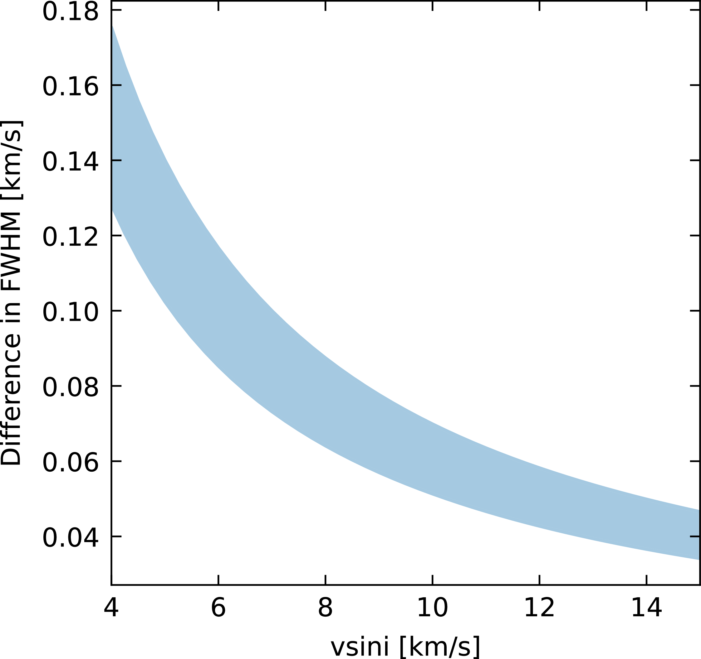
Then we simulated the broadening introduced by fibre offsets by stacking line profiles according to estimated offsets. Comparing the combined and theoretical profiles, the difference in full width at half maximum (FWHM) gives an estimation of the broadening magnitude. As presented in the Figure B6, the effect is strongest for stars with low
 $v \sin i$
and can exceed 1% when
 $v \sin i \lt 8.5 \mathrm{km\,s^{-1}}$
.
Simulated difference between the FWHM of a combined line profile and a theoretical profile versus
 $v \sin i$
. The range of estimated broadening at each projected rotational velocity reflects different velocity steps as the wavelength changes across orders.

 ∼
 7×7
 λ
 τ
 τ
 τ
 τ
 τ
 τ
 τ
 Teff=5300
 logg=4.48
 [Fe/H]=−0.55
 ξ=0.91
 −1
 ζ=3.62
 −1
 vsini=0.1
 −1
 R=75000
 −0.09
 ±1
 vsini

 Open access

