

In recent times, a consensus has emerged that low and stable inflation is essential for economic growth and development. Governments have adopted a variety of monetary policy strategies to combat inflation, including most notably the granting of independence to the central bank and the adoption of a fixed exchange rate. However, an alternative strategy known as “inflation targeting” (IT) has been receiving an increasing amount of attention from policymakers and central bankers, including U.S. Federal Reserve Chairman Ben Bernanke. IT is a transparent monetary policy rule in which the central bank commits to using monetary policy solely for the purpose of meeting a publicly announced numerical inflation target within a particular time frame. Since 1989, some twenty-five countries have adopted IT as a monetary policy rule, and the evidence thus far suggests that it is an effective inflation-fighting strategy.1
In a recent publication, the International Monetary Fund (IMF) reported that an additional twenty countries were seeking technical assistance from the IMF's staff to implement IT, and that ten were expected to adopt a formal inflation target within the next five years.2IMF 2006.
Ibid., 3.
The emergence of IT presents a puzzle for scholars of international political economy and central banking, and it exposes a weakness in the dominant analytical framework for the study of monetary policy. It is surprising that IT has been almost completely ignored by political scientists. The political economy literature sets up a dichotomy between one monetary policy rule—a fixed exchange rate—and the alternative of central bank independence as solutions to the time-inconsistency problem in monetary policy.4
The framework comes from a seminal special issue of International Organization, including contributions by Bernhard, Broz, and Clark 2002; Bernhard and Leblang 2002; Broz 2002; Clark 2002; Freeman 2002; Frieden 2002; Hallerberg 2002; and Keefer and Stasavage 2002.
The question of monetary policy rules has grown more salient as countries have abandoned fixed exchange rates in the wake of currency crises and speculative pressures. For example, foreign exchange pressures forced Britain and Sweden to terminate their exchange rate pegs in the early 1990s, and both countries promptly turned to IT as an alternative nominal anchor.6
Bernanke et al. 1999.
IMF 2006.
Calvo and Reinhart 2002.
The increasing popularity of IT is not limited to emerging-market countries or to countries experiencing exchange rate crises. Indeed, the first country to adopt IT was New Zealand in 1989, which had abandoned its pegged exchange rate four years earlier. More recently, Norway transitioned from a decade of managed floating to an inflation targeting regime in 2001.10
Soikkeli 2002.
The U.S. Federal Open Market Committee (FOMC) discussed the possibility of adopting an inflation target, and the expected resistance from members of Congress to such a move, during its meeting on 27–28 June 2000. See FOMC 2000. More recently, Federal Reserve Chairman Bernanke has advocated the adoption of IT. See Bernanke 2003.
The apparent resistance to a formal inflation target by U.S. policymakers is a reminder that IT is not politically palatable in all countries or at all times; indeed there is striking variation in the adoption of IT around the world. Some countries continue to conduct monetary policy with no nominal anchors in an environment of flexible exchange rates. Aside from the United States, these countries include Argentina, Japan, Malaysia, and Switzerland, among others. The variation in the adoption of IT therefore presents a puzzle for scholars of monetary policy institutions. Economists have focused on the macroeconomic consequences of IT, but there has been little systematic research on the political and economic determinants of the adoption of IT around the world.12
Studies of the macroeconomic effects of IT include, inter alia, Ball and Sheridan 2003; Levin, Natalucci, and Piger 2004; Truman 2003; and the empirical studies in Loayza and Soto 2002. Truman 2003 includes a separate analysis of IT as a dependent variable that focuses primarily on economic variables, including domestic economic conditions, exchange rates, and central bank independence. Bernanke et al. 1999 includes a number of case studies of countries that adopted IT; some of those cases touch on political factors, but no systemic assertions are made with regard to the influence of politics or institutions on the adoption of IT. Gerlach 1999 attempts a more systematic analysis of the influence of central bank independence and EU membership on the choice of IT, but his cross-sectional research design (with only twenty-two observations) limits the significance of his findings.
The goal of this article is to explain the variation in the adoption of IT around the world. We begin by constructing a simple model based on the Barro-Gordon framework.13
Barro and Gordon 1983.
This article proceeds as follows. In the next section, we provide a literature review and an explanation of IT as a nominal anchor for monetary policy. We then derive testable claims from a formal model of the government's choice of adopting IT that incorporates factors such as the central bank's institutional mandate, partisanship, and the trade-offs inherent in monetary policymaking. In the third and fourth sections, we present the data, statistical models, and results that are used to test our claims. We conclude by discussing the implications of our findings for the study of central banking and monetary policy, and offer guidance for future research.
Inflation Targeting: A Brief Primer
Inflation targeting is a monetary policy framework in which the government and/or the central bank announces an official numerically specified target for inflation over a given time period.14
The inflation target may be a specific level (for example, 2 percent) or a range (for example, between 1 and 3 percent). Accompanying the target is a public commitment to price stability as the primary or overriding goal of monetary policy, and a promise to hold central bankers accountable should they fail to meet the inflation target. The practice of IT requires the central bank to publish inflation forecasts on a regular basis, and to maintain transparency about its strategies for keeping inflation in check.15Svensson 1997.
An inflation target is a “nominal anchor” for monetary policy. Just as a fixed exchange rate serves to anchor the public's expectations of inflation, so too does an inflation target serve as a visible signal of the central bank's monetary policy goals. The public at large is acutely aware of changes in the price level; individual consumers may not have the capacity to ascertain day-to-day changes in the price indexes used by central banks, but they certainly do feel the pinch of higher (or lower) prices in housing, durable goods, and consumer products over time. Unlike alternative quantitative targets for monetary policy, such as the money supply, an inflation target lends itself to public monitoring. If a central bank fails to meet its stated inflation target, it cannot hide from public reproach. The publication of inflation forecasts and current macroeconomic conditions by the central bank strengthens the public's ability to monitor the central bank's policy decisions.
The emergence of IT coincides with the breakdown of the Bretton Woods international monetary system in the early 1970s and the relative decline in the popularity of fixed exchange rates. In 1985, fixed exchange rates accounted for more than 50 percent of developed country monetary policy regimes and 75 percent of developing (nonindustrial) country regimes; in 2005, the respective figures were 5 percent and 55 percent, with further declines expected in the short term.16
IMF 2006.
Husain, Mody, and Rogoff 2005.
Levy-Yeyati and Sturzenegger 2003.
Husain, Mody, and Rogoff 2005.
With the decline in the popularity of exchange rate pegs, many countries have searched for alternative nominal anchors to keep inflation under control. Early attempts to target the money supply were largely unsuccessful, in part because central banks did not view monetary targets as a serious commitment to low inflation.21
Mishkin 2000.
IMF 2006.
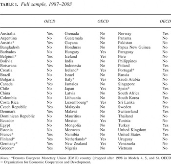
Full sample, 1987–2003

Bernanke and his colleagues are quick to note that IT does not constitute a hard-and-fast monetary policy rule. Indeed, they prefer the term “constrained discretion” to describe the combination of the explicit numerical target—which clearly guides the central bank's policy decisions—along with the flexibility retained by the central bank to address short-term exogenous shocks and unforeseen circumstances.25
However, they also note that there is “no such thing in practice as an absolute rule for monetary policy,” and that discretion is a part of every monetary policy framework, even the austere classical gold standard of the nineteenth century.26Bernanke et al. 1999, 5.
Empirical studies of the macroeconomic impact of IT have grown increasingly optimistic about its effectiveness in fighting inflation. Truman, for example, conducts a large-sample analysis and finds that countries that adopt IT have lower inflation levels, controlling for a battery of economic controls.27
Truman 2003.
Levin, Natalucci, and Piger 2004.
Ball and Sheridan 2003.
IMF 2006.
The Model: Loss Functions and Sequence of Moves
We construct a simple open-economy monetary-policy model to explain when countries are likely to adopt an inflation target as a nominal anchor for monetary policy. We begin with the standard assumption that monetary policy involves a short-run trade-off between maintaining low inflation and expanding output to reduce unemployment. There are three actors in the model: the central bank, the government, and private-sector wage-setters in the economy. The model focuses on how strategic interaction between the central bank and the government affects the adoption of an inflation target, given that wage-setters in the economy form their expectations about future inflation rationally. This approach is consistent with the existing literature, which demonstrates that central banks and government leaders jointly determine whether or not to adopt IT.31
As emphasized by Agénor, the choice and implementation of an inflation target “typically represents an understanding between the government and the governor (or president) of the central bank.”32Agénor 2001, 42.
See, for example, Mishkin and Westelius 2006; Persson and Tabellini 2000; and Waller and Walsh 1996.
Nineteen out of a total of twenty-two IT countries in our sample had a de facto floating exchange rate for several months (in some cases a few years) before adopting IT. As emphasized by the IMF 2006, all of these countries faced a choice of either discretion via the float or IT technology before actually adopting IT.
We present the model below systematically in four steps. First, we define the government's loss function. We then describe the economy's output function and how wage-setters set wages in the economy. Second, we define the central bank's loss function and formalize how its institutional mandate affects its strategic behavior. Third, we describe the sequence of moves in the model. Fourth, we present the model's equilibrium result and comparative static predictions from which we derive our main testable hypothesis.
Following the extant literature,36
See, for example, Barro and Gordon 1983; Keefer and Stasavage 2003; Persson and Tabellini 2000; and Scheve 2004.

where L denotes a left-leaning government and R indicates a right-leaning government. In (1), θG is the weight that the government places on controlling inflation and thus captures the government's aversion to inflation.37
We allow θG to be unbounded (θG ∈ [0,∞]) to avoid imposing an artificial upper bound on θG.
See Alesina and Rosenthal 1995; Alesina, Roubini, and Cohen 1997; Bearce 2003; Franzese 1999; and Oatley 1999.
The expression (y − y)2 in equation (1) captures deviations of output from the output target. Output in the economy follows from the familiar “Lucas-style” specification and is assumed to be a function of surprise inflation engineered by a policymaker and a supply shock that is normally distributed with mean 0 and variance σε2:

Equation (2) implies that the natural level of output is normalized to 0 (in log). As in standard monetary-policy models, the supply shock can be observed by the government and the central bank (whose loss function is defined below) but not ex ante by wage-setters. Observe that since workers in the economy are rational and wish to preserve their purchasing power, they claim a nominal wage in their wage contract that covers the expected price level πe. Since wage-setters know that workers wish to preserve their purchasing, they will set wages equal to expected inflation:

where E(.) is the expectations operator.39
Wage-setters in the economy thus form their wage expectations before supply shocks are realized.
Barro and Gordon 1983. Let e = π and et−1 = πt−1. Substituting e = π and et−1 = πt−1 in equation (1) and taking the first-order condition of equation (1) with respect to e yields ∂LG /∂e = e − et−1 − θGα, which leads to e = et−1 + θGα where α is the weight that the incumbent places on minimizing the output gap.
We now describe the central bank's loss function. Unlike the monetary-policy models in the literature, which assume that the central bank's preferences on inflation are unknown and are therefore a stochastic parameter,41
we suggest that the central bank's institutional mandate is one indicator of its inflation preferences. In particular, following extant studies that examine the central bank's role as a bank regulator, we argue that central banks that hold or share bank regulatory authority are functionally responsible for maintaining the stability and profitability of the commercial banking sector, and are therefore less likely to alter interest rates solely on the basis of price-stability objectives.42On the regulatory responsibilities of central banks, see Barth, Caprio, and Levine 2006; and Copelovitch and Singer forthcoming. On the trade-off between price stability and bank stability, see Cukierman 1991.
Frieden 1991.
Clearly no central bank with regulatory responsibility wants to preside over an environment of declining bank profits or bank instability. We therefore expect central banks with bank regulatory responsibility to be more sensitive to bank stability when setting monetary policy than central banks without such responsibility.46
Copelovitch and Singer forthcoming.
Empirical studies have demonstrated that combining monetary policy and bank regulatory responsibilities in one agency leads to higher inflation for a large panel of countries since the 1970s.47
See ibid.; and Posen 1995. Results from error correction models in our sample of seventy-eight countries (1987–2003)—available from the authors on request—show that the level and change in logged inflation in countries where the central bank does not have bank regulatory responsibilities is statistically lower than in countries where the central bank has regulatory authority.
Cecchetti and Ehrmann 2001.
Ibid. For a description of the SVAR model and its application to studies of inflation aversion, see Cecchetti, McConnell, and Quiros 1999; and Cecchetti and Ehrmann 2001.
Difference-of-means tests reveal that the average level of inflation aversion among central banks that do not have bank regulatory responsibilities (0.63) is significantly higher than those with bank regulatory responsibilities (0.39, p = .000). Results from the estimated SVAR models are not reported to save space but are available on request.
The central bank's institutional mandate enters its loss function in our model via the parameter λ that takes the value of 1 if the task of bank regulation has been separated from the central bank's monetary policymaking functions, and 0 otherwise. We assume that an inflation target, πT, can be used as a commitment device to maintain low inflation.51
Svensson 1997.

where (y − y)2 captures deviations of output from the output target, while the parameters πT and λ were described above.
The parameters y, λ, and πT in equation (4) are also typically incorporated in the players' loss functions in extant models.53
See, for example, Clark 2002; Cukierman 1992; Mishkin and Westelius 2006; and Waller and Walsh 1996.
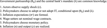
At the beginning of the period, actors observe the supply shock ε. The government's partisanship θG (G ∈ {L,R}) and the central bank's institutional mandate (λ) are common knowledge to all the actors. After observing ε, the policymakers either adopt or do not adopt IT, conditional upon government partisanship and the central bank's institutional mandate. Then wage-setters in the economy form inflation expectations based on whether or not IT is adopted and lock into nominal wage contracts with workers for the remainder of the period. Subsequently, the policymakers choose monetary policy. Finally, inflation (π) and real output (y) are realized. The sequence of moves described above is illustrated in Figure 1.

Sequence of moves
Results and Testable Hypothesis
We state and describe two main results here that are derived from our model. The first result formally describes the monetary policy outcomes of inflation and output in two cases: (i) a hypothetical discretionary case where the government unilaterally sets inflation and output in the absence of any commitment technology, and (ii) the Nash equilibrium monetary policy outcome that results from the strategic interaction between the government and the central bank. The second result, which is the model's main substantive result, posits the political and institutional conditions under which an inflation target is more likely to be adopted.
We begin the presentation of the theoretical results by stating the formally the first result from our model:
Lemma 1: (i) In a discretionary equilibrium, where the government neither consults the central bank nor uses any other commitment technology, inflation is given by πG = y/θG − ε/1 + θG and output y = εθG /(1 + θG). The government's expected loss in the discretionary case is:

(ii) When the government's preference parameter with respect to inflation is given by θG,G ∈ {L,R}, and the central bank's loss function is defined by equation (4), the Nash equilibrium inflation and output level is


Proof.
See Appendix.
The inflation level in part (i) reveals the standard inflationary bias that occurs in the discretionary case.55
Because θR > θL, the resulting inflation even in the discretionary case will be lower under right-leaning governments compared to leftist governments; that is πR < πL.
Proposition 1: The likelihood that an inflation targeting regime is adopted will increase under a right-leaning government if the central bank does not have bank regulatory responsibilities (more formally, π* = πT for λ = 1 and θG = θR).
Proof.
See Appendix.
The result in proposition (1) is derived from two exercises conducted on the Nash equilibrium solution described earlier. First, given our assumption that right-leaning governments prefer lower inflation, we study how the Nash inflation solution π* is affected when a right-leaning incumbent is in office. Second, we examine how the Nash inflation level is influenced when the central bank does not have bank regulatory responsibility in its mandate (λ = 1). The result from these exercises is that neither a right-leaning government nor a central bank without bank regulatory authority can unilaterally determine the choice and implementation of an inflation target. Rather, it is the combined effect that matters: an inflation targeting regime is more likely to emerge if a right-leaning government is in office and if the central bank does not have bank regulatory authority. Further, proposition (1) also suggests that a right-leaning government and a nonregulatory central bank have no incentives to deviate from an inflation targeting regime in equilibrium and will thus maintain IT.
The intuition behind this result has four components. First, as suggested earlier, both right-leaning governments and central banks without regulatory authority are especially interested in keeping inflation in check. The compatibility of preferences over inflation fosters mutual agreement between these two parties on using a formal inflation target, which substantially enhances the credibility of the government's commitment to low inflation. A right-leaning government and a nonregulatory central bank will mutually recognize ex ante that the ex post expected losses under IT will be lower than losses without IT.56
See the proof of claim (1) in the Appendix.
The closed form solution of πT* is given in the proof of part (ii) of lemma (1) in the Appendix.
An additional comparative static result (demonstrated in the Appendix) suggests that IT is less likely to be adopted when a left-leaning incumbent is in office.58
See the proof of claim (2) in the Appendix.
For evidence on this claim, see, for example, Alesina, Roubini, and Cohen 1997.
The preceding discussion leads to the following testable hypothesis:
Hypothesis 1: The likelihood of adopting IT increases under a right-leaning government if the central bank does not have bank regulatory responsibilities.
Statistical Methodology: The Spatial Autoregressive Probit Model
To test the prediction in hypothesis (1), we employ a spatial autoregressive (AR) probit model for TSCS data. The spatial AR probit model is appropriate for two reasons. First, the dependent variable is country i's binary choice of adopting IT at time t, thus making a probit model a logical choice. Second, there may be reason to expect that policy diffusion processes are at work, given that IT is a new technology for monetary policymaking.61
On international diffusion, see Brinks and Coppedge 2006; Brune and Guisinger 2006; Franzese and Hays 2006; and Simmons and Elkins 2004.
Anselin 2001.
We briefly describe the spatial AR probit model here. Suppose that there are i = 1,2,… N countries observed at time periods t = 1,2,3…T, where yit* is the latent version of the observed binary dependent variable yit such that

The first-order spatial lag (or spatial autoregressive) probit model in vector form, stacking cross-sectional observations over all time periods is:

where X is a (TN × K) matrix of exogenous variables that includes the independent variables we use to test hypothesis (1). The scalar ρ in equation (9) is a spatial lag coefficient and reflects positive spatial correlation in the dependent variable if ρ > 0, negative spatial correlation if ρ < 0, and no spatial correlation if ρ = 0. More substantively, the estimate of ρ statistically captures the impact of diffusion on the likelihood of adopting IT. If diffusion processes drive the adoption of IT, the estimate of ρ will be positive.
In equation (9), W(l) is a (TN × TN) block diagonal matrix having T copies of an (N × N) spatial lag weights matrix W along the diagonal. The individual entries Wij in W capture the spatial interconnectedness between countries i and j in W and thus account for the potential role that diffusion may play in influencing IT. We describe below how we operationalize Wij. Finally, ε is a spatial autoregressive error term, where v is a (TN × 1) vector of i.i.d. random variables with 0 mean and covariance matrix σ2v, and λ is a scalar that measures spatial error correlation. λ > 0 (λ < 0) indicates that the errors are positively (negatively) correlated, and λ = 0 indicates that the errors are not correlated.63
The spatial autoregressive error term is a nuisance parameter in that it captures spatial autocorrelation in measurement errors; see Anselin and Bera 1998. Hence the estimate of ε cannot be used to interpret the diffusion of IT.
Many weighting schemes have been used to operationalize wij in spatial regression models by political scientists. For example, Franzese and Hays code wij = 1 for countries i and j that share a border and wij = 0 for countries that do not, while Brune and Guisinger and Simmons and Elkins employ a variety of diffusion variables, including directed trade-flow shares and sovereign bond ratings.64
Since the diffusion of IT is typically characterized by neighbor effects rather than a competition for global capital, we use a geographic measure of spatial contiguity operationalized as the inverse distance between states i and j, where wij = 1/dij. As the distance between states i and j increases (decreases), wijdecreases (increases), thus giving less (more) spatial weight to the state pair when i ≠ j. We use a “minimum distance database” of the shortest distance between the two closest physical locations for every pair of independent polities in the world.65See Gleditsch and Ward 2001 and 2006. The database records the shortest distance in kilometers between points on the outer boundaries for two polities, regardless of whether the states are separated by land or sea, given the borders in place in a particular time period. We updated their database for the countries in our sample until 2003.

Note that the model cannot be estimated by standard maximum likelihood methods. Difficulties arise from the fact that we no longer have the product of n independent univariate standard normal probabilities, but instead we need to evaluate an n-dimensional multivariate integral to compute the joint probabilities appearing in the likelihood. The Appendix describes the Bayesian Markov Chain Monte Carlo (MCMC) methods used to estimate the model, the procedure used to correct for heteroskedasticity, and the log-likelihood of the spatial AR probit model.66
The spatial AR (lag and error) probit model is estimated using the MATLAB toolbox from LeSage 2000.
Data and Dependent Variable
We compiled a TSCS data set for seventy-eight countries from the developed and developing world from 1987 to 2003 to test the prediction in hypothesis (1). Of these seventy-eight countries, thirty are Organization for Economic Cooperation and Development (OECD) countries and the remaining forty-eight are non-OECD countries (see Table 1). We selected 1987 as the first year in which IT was an available option, given that New Zealand was the first to adopt IT two years later in 1989. The results of our econometric models are robust to extending the sample back to years before 1987.
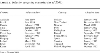
In accord with the formal model, we operationalize the dependent variable inflation target as a dichotomous measure that takes the value of 1 if a country has formally adopted a numerical target for inflation, and 0 otherwise. The variable is taken from Truman67
Truman 2003.
Fatas, Mihov, and Rose 2007.
Ibid.
Inflation targeting countries (as of 2003)

We first estimate the spatial AR probit model on our entire sample of seventy-eight countries (1987–2003) in Table 1. Second, since non-OECD and OECD countries often differ along various dimensions (the level of development, the degree of real effective exchange rate volatility, and so forth), we divide our global sample into OECD and non-OECD subsamples and test our hypotheses within each group. Third, as a robustness test, we drop all twelve Eurozone countries from our sample from 1999 onward, because their inclusion as independent observations is dubious in light of their delegation of monetary policy authority to one supranational central bank.70
In the sample where the twelve EMU countries are dropped from 1999 onward, we code Finland and Spain as inflation targeters from 1993 and 1995 (respectively) up until they adopted the Euro in 1999. Econometric issues aside, the coding of the European Central Bank (ECB) as an inflation targeter by Fatas, Mihov, and Rose 2007 is debatable. The ECB marries its numerical definition of price stability (under 2 percent inflation) with a policy strategy that emphasizes a quantitative assessment of money supply growth.
Independent and Control Variables
The first independent variable, separate, takes the value of 1 if the central bank is not responsible for bank regulation, and 0 for all other cases, including when the central bank is the sole bank regulator or when it is one of multiple regulators (as in the United States).71
Data on this variable come from Bank for International Settlements 2005; Bankers' Almanac 2005; Barth, Caprio, and Levine 2003; and Copelovitch and Singer forthcoming.
The second independent variable is government partisanship from the World Bank's Database of Political Institutions (DPI).72
Beck et al. 2001.
We rescaled the right to left scale of partisanship in the DPI to a left to right scale to facilitate testing of the prediction in hypothesis (1) and aid interpretation of the estimated results.
We include a number of economic control variables in the model. First, scholars have suggested that an increase in the volatility of economic growth encourages governments to adopt IT to induce economic stability.74
Svensson 1997.
Data for these economic controls come from IMF 2004.
High real interest rates typically reflect dissatisfaction with current economic performance and increased inflationary expectations, and may prompt policymakers to adopt IT. We include real interest rate, measured in percentage terms as (1+ nominal interest rate/1 + inflation rate) −1 in the specification and expect that its effect will be positive.76
Data come from ibid.
The data used to construct this variable come from Reinhart and Rogoff 2004.
Governments in countries with a poor current account position might attempt to finance a large deficit by following expansionary monetary policies and thus will avoid adopting IT. We include current account position (calculated as a percentage of nominal GDP) and expect that its impact will be negative. We control for gdp per capita, given large variation in income levels across countries in our sample and the possibility that this could affect monetary policy. It has been suggested that greater trade openness may make it harder for authorities to tie their hands to an inflation target.78
IMF 2006.
Data for these variables come from World Bank 2004.
We include a dummy for floating exchange rate regime. This variable is expected to have a positive effect since countries that float their currency may favor using an inflation target as a nominal anchor for monetary policy.80
IMF 2006.
Reinhart and Rogoff 2004 use parallel market exchange rates, foreign reserve movements, and country chronologies to determine the actual operation of an exchange rate regime over time. Reinhart graciously provided an updated version of the data set to the authors.
In addition to the economic controls, we include a number of political and institutional controls in the specification. First, governments in parliamentary democracies may find it politically easier to adopt IT since the executive-legislature divide in such democracies is usually less pronounced, therein facilitating adoption of new monetary policy rules.82
Linz and Valenzuela 1994.
Data are from Beck et al. 2001.
O'Mahony 2007.
Bernhard, Broz, and Clark 2002.
The Cukierman, Miller, and Neyapti 2002 index is a composite measure of sixteen different aspects of central bank statutes including, for example, the relative autonomy between the government and central bank, and the scope of decision making in monetary policy.
We also control for the degree of transparency of political institutions with the polity iv index.88
The Polity IV measure for regime type ranges from −10 (denoting a full autocracy) to +10 (denoting a full democracy). Following Broz 2002, we subtract the Polity IV “democracy” score from the “autocracy” rating for each observation; this constitutes the Polity IV index in our model.
Rosendorff and Vreeland 2006.
Broz 2002.
Beck et al. 2001.
Findings and Analysis
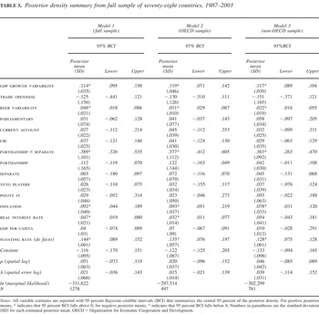
Table 3 presents the results obtained from estimation of the spatial AR probit model via Bayesian MCMC methods. Model 1 is based on the full sample of countries, while Models 2 and 3 are limited to OECD and non-OECD countries, respectively. Following standard Bayesian terminology and techniques, we report the posterior mean and standard deviation (reported in parentheses in the table) for each variable. The estimates of the variables in each model are reported with 95 percent Bayesian credible intervals (BCI).
Posterior density summary from full sample of seventy-eight countries, 1987–2003

The estimated posterior mean of the interaction term partisanship × separate in Model 1 is positive and significantly different from 0 (with the 95 percent BCI falling above 0), indicating that the combined effect of a right-wing incumbent and a nonregulatory central bank increases the likelihood of adopting and maintaining an inflation target.93
In discussing the results, we use frequentist terms such as “significant” or “insignificant” to facilitate interpretation of the reported results.
We estimated an additional spatial AR probit model where we dropped partisanship × separate but retained the individual components of this interaction term and other controls. The results, available on request, show that separate and partisanship remain individually positive, but insignificant.
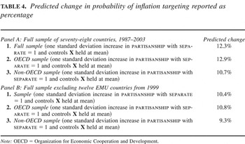
Predicted change in probability of inflation targeting reported as percentage


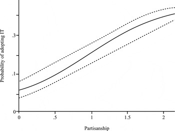
Predicted impact of partisanship on adopting IT (when separate = 1)
As mentioned earlier, we divided our sample into two separate subsamples of OECD and non-OECD countries, and estimated the baseline specification in Model 1 for each of these two subsamples. The estimated posterior mean of partisanship × separate is positive and significantly different from 0 in the OECD sample (Model 2) and the non-OECD sample (Model 3). Much like the global sample, the constitutive components of our key interaction term separate and partisanship are each insignificant in the two subsamples. Substantively, we find that when separate is set equal to 1 and the other variables in the specification are held at their means in the respective models, increasing partisanship by one standard deviation above its mean increases the likelihood of adopting IT by 12.9 percent in the OECD sample and by 10.7 percent in the non-OECD sample.
Interestingly, the posterior mean of the spatial lag of the dependent variable, ρ, is insignificant in Models 1, 2, and 3. This implies that there is no statistical support for the alternative explanation that international diffusion effects—captured by physical distance between countries or trade relations—drive the adoption of IT.95
The estimated posterior mean of the spatial AR error parameter is also insignificant in all the models.
Alternative political variables that may account for the choice of an inflation target are not significantly different from 0. In particular, polity iv, veto players, cbi, and the parliamentary dummy are insignificant in all three models. These findings support the argument that IT can be flexibly adapted to a variety of political environments, including levels of democracy, the type of democracy (presidential versus parliamentary), veto players, and central bank independence.96
Unlike the political controls, the economic control variables fare better in the estimated models. For instance, the estimated posterior mean of gdp growth variability and inflation are positive and significant in each model. Likewise, the posterior means of real interest rate and reer variability are consistently positive and significant. However, trade openness and gdp per capita are both insignificant in each model. In sharp contrast, we find that the estimated posterior mean of the floating exchange rate variable is positive and significant in the empirical models for the global, OECD, and non-OECD samples, thus indicating an association between floating exchange rates and the adoption of IT. This finding confirms the notion that IT is an alternative, not a complement, to fixed exchange rates.
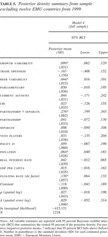
We conducted a number of robustness tests and diagnostics to check the econometric validity of the empirical results described above. First, we exclude the twelve countries in the EMU beginning in 1999 and estimate the spatial AR probit model for this reduced sample. The posterior mean of partisanship × separate remains positive and significant in the empirical model estimated for the reduced sample (see Model 4 in Table 5). Furthermore, the estimates of the individual components of the aforementioned interaction terms are insignificant in Model 4. The substantive effect of partisanship × separate from Model 4 is reported in Table 4, Panel B. When separate is set equal to 1 and the other variables are held at their means, increasing partisanship by one standard deviation above its mean increases the likelihood of adopting IT by 10.4 percent. Thus hypothesis (1) finds strong statistical and substantive support in the sample where we exclude the twelve EMU countries from 1999. We then divide this reduced sample into separate subsamples of OECD and non-OECD countries, and estimate the spatial AR probit model for each group. The results from this empirical exercise are not reported to save space, but we find strong statistical support for hypothesis (1) in the group of OECD and non-OECD countries from the reduced sample.97
These results are available from the authors on request.
Posterior density summary from sample excluding twelve EMU countries from 1999

We also checked for specification robustness by adding the following variables to each model in Tables 3 and 5: the temporal lag of the dependent variable, inflation volatility, real gdp gap, government polarization and financial depth. Inclusion of these variables did not substantively or significantly alter any of the results reported in Tables 3 and 5.98
These results are available from the authors on request.
Gourieroux, Monfort, and Trognon 1982.
Conclusion
The premise of this article is that the adoption of IT is a political decision within the context of monetary policymaking. In today's environment of global finance, fixed exchange rates are often not a viable option for fighting inflation. Thus, governments must make important decisions about monetary policy. Political scientists have largely focused on one strategy—granting political independence to the central bank—as an alternative to fixed exchange rates. This article demonstrates that governments have an additional decision to make: whether or not to impose a transparent monetary policy rule on the central bank. We argue that countries are more likely to adopt IT when there is a conformity of preferences for low-inflation monetary policy between the government and the central bank. The central bank's regulatory mandate—that is, whether or not it is tasked with regulating the banking sector—is one important indicator of its monetary policy preferences, since regulatory central banks are likely to be more sensitive to financial stability concerns when setting interest rates. The monetary preferences of the government are best reflected by the incumbent's partisanship, as right-leaning governments are generally more partial toward price stability than their left-leaning counterparts. Countries are therefore more likely to adopt IT when there is a right-leaning administration combined with a central bank that is not directly responsible for bank regulation. On the other hand, we find that left-leaning governments and central banks with bank regulatory responsibility are unlikely to favor IT. The results of our spatial AR probit model on data from seventy-eight countries from the 1987–2003 period provide strong evidence of our arguments.
Recent scholarship on the global economy argues that diffusion processes are a potent and frequently overlooked influence on domestic economic policymaking.100
It is therefore reasonable to ask whether the behavior of neighboring countries influences a country's decision to adopt IT. The spatial AR probit model used to analyze our TSCS data set explicitly accounts for spatial dependence in the dependent variable, and results from the model provide no statistical support for international diffusion processes. Domestic factors appear to be the driving force behind the adoption of IT. However, future research will determine whether the alternative diffusion channels specified in the literature on financial liberalization are applicable to the spread of IT.Our findings challenge the conventional dichotomy between fixed exchange rates and central bank independence and also provide a potential explanation for the mixed performance of central bank independence alone as a predictor of inflation outcomes. IT provides a transparent nominal anchor for monetary policy. Thus, a central bank with an explicit inflation target is likely to behave differently from a central bank with complete autonomy in setting monetary policy goals. At a minimum, scholars should be careful to consider the presence or absence of IT when discussing the institutional structure of the central bank. Central bank independence captures only part of the full picture.
This article certainly does not constitute the last word on the politics of IT. Indeed, the intent of the article is to spur more research on a critical monetary policy strategy that has been overlooked by political scientists. More research is needed on the inflation preferences of governments and central banks, and on the tension between financial regulation and monetary policy. Moreover, there may be additional constituencies in favor or against IT that are not captured in our empirical analysis. Given that the IMF and many academic economists have adopted a decidedly positive stance toward IT, it behooves political scientists to examine the politics behind its implementation.
Appendix
Proofs of Model
Proof of Lemma 1, Part (i).
The first-order condition of the government's loss function in equation (1) with respect to π given the Lucas supply curve in equation (2) is:

Taking expectations in equation (A1) and using the resulting πe yields after some algebra πG = y − (ε/1 + θG). From the first-order condition of the government's loss function in equation (1) with respect to y, we obtain (∂UG /∂y) = y − y = 0, which ⇒ y = y. Substituting y with y in πG and solving for the discretionary output yields y = ε/(1 + θG). Substituting πG and yG in the loss function in equation (1) and taking expectations yields the expected losses under discretion E([ell ]G) = ½[(y)2[θG /(1 + θG)] + σε2[θG /(1 + θG)]].
Proof of Lemma 1, Part (ii)
The first-order condition of the central bank's loss function in equation (3) with respect to π given the Lucas supply curve and the government's relative aversion for inflation θG is:

Taking expectations as given and using the resulting πe yields the Nash equilibrium level of inflation π* = πT + y(1 − λ) − [λε/(1 + θG)]. From the first-order condition of the loss function in equation (3) with respect to y, we get (∂UCB /∂y) = y(1 − y) + y(λ − 1) = 0, which implies that y = y. Solving for the Nash equilibrium output using the Lucas supply curve yields y* = [ελ/(1 + θG)] − (λy/θG). Substituting π* and y* in equation (1), we find that the optimal value of πT* that minimizes E([ell ]G) is πT* = −(y/θG).
Proof of Proposition 1.
Under a right-leaning incumbent, θG = θR, which ⇒ π* = πT + y(1 − λ) − [λε/(1 + θR)]. By construction θR strictly increases under a right-leaning incumbent because he or she is more concerned about keeping inflation in check. Therefore, in the limit θR → ∞ (this captures strictly increasing θR), π* converges to limθR→∞ π* = πT + y(1 − y). From π* = πT + y(1 − λ) that π* = πT if λ = 1. Hence π* = πT for θR → ∞ and λ = 1. For λ = 1, the first-order condition of the loss function in (3) w.r.t π is (∂UCB /∂π) = (θR + 1)(π − πT) = 0, which ⇒ π = πT(θR + 1)/(θR + 1) and π* = πT for λ = 1 and ∀θR > 0.
Proof of Claim 1.
Substituting the optimal IT rule πT* in π* and then substituting the resulting expression as well as y* in the government's loss function in equation (1) and taking expectations yields after algebra the expected losses under IT: E([ell ]IT) = 1/2{(y)2(θG2 + λ(1 + θG)/θG2) + σε2(λ + θG /1 + θG)}. Since λ = 1 for a nonregulatory central bank, E([ell ]IT) = 1/2{(y)2(θG2 + 1 + θG /θG2) + σε2(1 + θG /1 + θG)}, which after simplification is E([ell ]IT) = 1/2{(y)2(1 + (1 + θG /θG2)) + σε2}. Taking the difference between E([ell ]IT) and E([ell ]G) leads after algebra to E([ell ]IT) − E([ell ]G) = ((y)2/θR2) − σε2 + σε2(θR /1 + θR). Since θR → ∞ under a right-leaning incumbent, we get E([ell ]IT) − E([ell ]G) = −σε2 < 0, which ⇒ E([ell ]IT) < E([ell ]G).
Proof of Claim 2.
Under a left-leaning incumbent, θG = θL and for λ = 1 implying a nonregulatory central bank, π* = πT + y − ε/(1 + θl). By construction θL strictly decreases under a left-leaning incumbent because he or she is less concerned about keeping inflation in check. Hence, in the limit θL → 0, which captures strictly decreasing θL. For θL → 0 and λ = 1, one can easily check that π* does not converge to πT, that is, π* ≠ πT under a left-leaning incumbent, as claimed.
Heteroscedasticity Correction in Spatial AR Probit Model
Let the last two terms in the full model in equation (10), following Case,101
Case 1992.

The log-likelihood of the spatial AR probit model is therefore,

where X* = Z(I − ρW)−1X and Φ is the cumulative distribution function of a standard normal distribution.
Bayesian MCMC Estimation of Spatial Autoregressive Probit Model
Following the MCMC technique described by Smith and LeSage102
Smith and LeSage 2004.

The estimation task is to construct a Markov chain that samples from each conditional distribution in turn, conditioning on the parameters obtained in the previous step in the process, to eventually arrive at a sample of draws from the posterior distribution. To conserve space, we only state the conditional posterior distributions for the spatial parameters ρ,λ and the latent dependent variable y* from Smith and LeSage. The conditional posterior for ρ and λ are respectively


where e is (I − λW)y* − Xβ and (I − λW)|y* − Xβ| for the spatial AR probit model. These two conditional distributions have an unknown form, thus we employ a Metropolis-Hasting algorithm with rejection to sample directly from equations (A6) and (A7). The conditional distribution for y* in the heteroskedastic spatial AR lag and spatial AR error probit model is respectively


With the conditional distributions derived, the MCMC estimation proceeds as follows conditional on a set of starting values β0,λ0,vi,0,ρ0,σ02,y0*:
- Update the value for β by drawing β|λ0,vi,0,ρ0,σ02,y0* using the conditional distribution p(β|σu2,vi,ρ,λ,y*,X). Label the updated value β1.
- Update the value for λ by drawing λ|β0,vi,0,ρ0,σ02,y0* using the conditional distribution p(λ|β,vi,σu2,ρ,y*,X) and the Metropolis-Hastings algorithm. Label the updated value λ1.
- Update the value for σ2 by drawing σ2|β0,λ0 vi,0,ρ0,y0* using the conditional distribution p(σu2|β,vi,ρ,λ,y*,X). Label the updated value σ12.
- Update the value for ρ by drawing ρ0|β0,λ0,vi,0,σ02,y0* using the conditional distribution p(ρ|β,vi,σu2,λ,y*,X) and the Metropolis-Hastings algorithm. Label the updated value ρ1.
- Update the value for vi by drawing vi,0|β0,λ0,σ02,ρ0,y0* using the conditional distribution p(vi|β,σu2,ρ,λ,y*,X). Label the updated value σ12.
- Update the value y* for by drawing vi,0 y0*|β0,λ0,σ02,ρ0 vi,0 using the conditional distribution p(y*|β,vi,σu2,ρ,λ,X). Label the updated value y1*.
The list of steps is repeated a large number of times, and after a burn-in period the sequence of collected realizations represents a draw from the posterior distribution of the parameters. Inference is conducted by using simple means and standard deviations of the empirical posterior distribution.