1 Introduction
Laminar–turbulent transition in wall-bounded flows has traditionally been studied by considering the case of Blasius boundary layer and plane or axisymmetric Poiseuille flows, while less attention has been paid to pipe and channel flows in the so-called entrance region. The latter problem remains of fundamental importance to obtain a better understanding of transition in a channel or pipe, since differences between theoretical, numerical and experimental approaches are frequently attributed to flow development effects (see Draad, Kuiken & Nieuwstadt (Reference Draad, Kuiken and Nieuwstadt1998) for the pipe flow case, for instance). For uniform flow conditions and at sufficiently high Reynolds number, the entrance flow in a plane-parallel channel consists of two developing boundary layers separated by an inviscid core (see Van Dyke Reference Van Dyke1970). The boundary layers merge farther downstream at a distance proportional to the Reynolds number. They are subjected to a favourable pressure gradient due to the confinement effect, which will as a consequence stabilize the flow with respect to the so-called Tollmien–Schlichting mode.
The literature provides several examples of linear stability studies of the flow velocity profiles in the developing region based either on the parallel flow assumption or including some treatment of non-local effects (Chen & Sparrow Reference Chen and Sparrow1967; Garg & Gupta Reference Garg and Gupta1981; Hifdi, Touhami & Naciri Reference Hifdi, Touhami and Naciri2004; Biau Reference Biau2008). Hifdi et al. (Reference Hifdi, Touhami and Naciri2004) and Biau (Reference Biau2008) show that in the region far downstream where the developing flow has a universal character (see Asai & Floryan Reference Asai and Floryan2004), velocity profiles are more stable than the developed Poiseuille flow. Near the channel entrance, no general statement can be made on the stability properties since the base flow is sensitive to inlet conditions (Sadri & Floryan Reference Sadri and Floryan2002). For uniform inlet boundary conditions, Chen & Sparrow (Reference Chen and Sparrow1967) and Garg & Gupta (Reference Garg and Gupta1981) have found that velocity profiles in that region are also more stable than the Poiseuille profile. For a similar case, Buffat et al. (Reference Buffat, Le Penven, Cadiou and Montagnier2014) have recently shown by direct numerical simulations (DNS) that, while boundary layers near the entrance are linearly stable for exponentially growing modes, they may experience laminar–turbulent transition well before their achievement of fully developed flow (i.e. the Poiseuille flow solution). They show that transition is triggered by secondary instability of streaks (elongated regions of excess or defect of streamwise velocity), leading to a rapid breakdown to turbulence. In their study, streaks are generated by superimposing pairs of streamwise vortices inside the boundary layers at a certain distance past the channel entrance. The selected vortices correspond to the optimal linear response in terms of energy gain under the parallel flow approximation. The streaks are amplified due to the so-called lift-up mechanism (Landhal Reference Landhal1980) and, when nonlinearities come into play, they undergo strong effects of amplitude saturation and distortion.
In that way, the path leading to a turbulent flow highlighted by Buffat, Le Penven & Cadiou (Reference Buffat, Le Penven and Cadiou2011) exhibits a strong resemblance to the bypass scenario for a flat-plate boundary layer flow (see for instance Brandt & Henningson Reference Brandt and Henningson2002; Zaki & Durbin Reference Zaki and Durbin2005; Durbin & Wu Reference Durbin and Wu2007). Buffat et al. (Reference Buffat, Le Penven, Cadiou and Montagnier2014) also show that the fully developed turbulent regime downstream is similar to a turbulent channel flow. Despite these similarities, the bypass transition scenario observed by the latter authors differs in some points from previous DNS of streak breakdown. While it is commonly accepted that streak breakdown is often caused by sinuous instability (i.e. an antisymmetric pattern with respect to the low-speed streak), Buffat et al. (Reference Buffat, Le Penven, Cadiou and Montagnier2014) show that streaks experience a transient varicose instability (i.e. characterized by a symmetric pattern) near the inlet before being dominated by a sinuous motion.
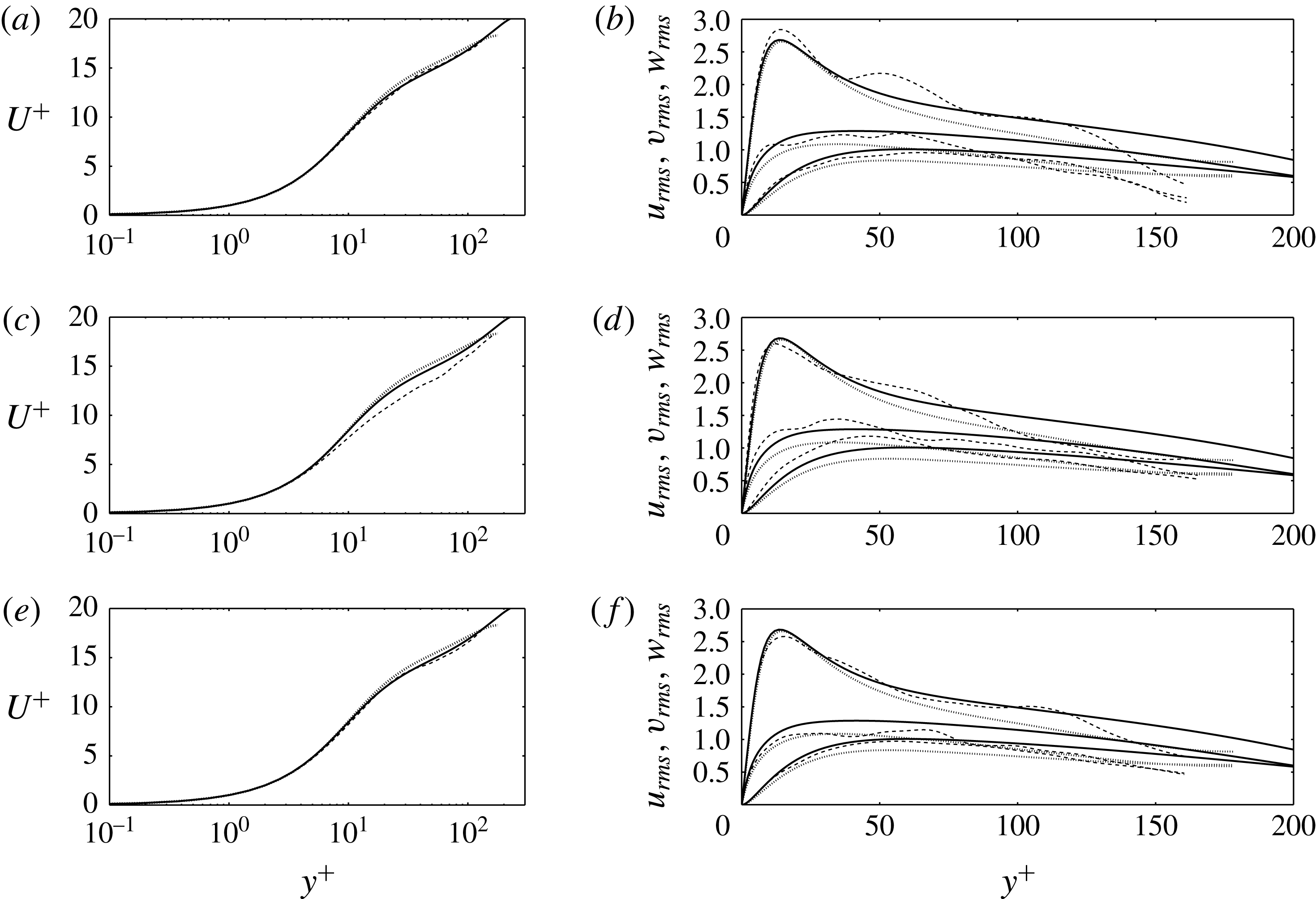
Andersson et al. (Reference Andersson, Brandt, Bottaro and Henningson2001) carried out the first linear stability analysis on steady boundary layer streaks, using the parallel flow approximation. They reported the onset of high-frequency modal secondary instabilities for critical streak amplitudes of 26 % and 37 % for the sinuous and varicose modes, respectively. The varicose instability is usually related to wall-normal inflectional velocity profiles, whereas the sinuous one seems to be concomitant to the presence of inflection points along the spanwise direction. This scenario is generally observed. However, Brandt (Reference Brandt2007) reported that for a specific low-speed streak shape, sinuous instability may be amplified due to the wall-normal shear. Nevertheless, discrepancies still remain between critical streak amplitudes predicted by modal linear stability theory and experiments, as reported by Matsubara & Alfredsson (Reference Matsubara and Alfredsson2001) and Mandal, Venkatakrishnan & Dey (Reference Mandal, Venkatakrishnan and Dey2010), where streak breakdown is observed for significantly lower streak amplitudes. In the past few years, many explanations have been addressed trying to fill the gap between theoretical and experimental observed thresholds. Vaughan & Zaki (Reference Vaughan and Zaki2011) and Hack & Zaki (Reference Hack and Zaki2014) suggest that discrepancies can be overcome by considering more realistic streaks (i.e. having a finite size in the streamwise direction and being unsteady). Brandt & de Lange (Reference Brandt and de Lange2008) show that streak collisions may lead to breakdown to turbulence for critical streak amplitudes lower than the ones predicted by a modal linear stability theory.
Finally, it is also clear that bifurcations of streaks may not necessarily be attributed to a secondary modal instability. Since the preliminary work of Schoppa & Hussain (Reference Schoppa and Hussain2002) that deals with streaks populating the near-wall region of a turbulent channel flow, a viable scenario relying on a breakdown mechanism triggered by the transient growth of secondary perturbations has emerged. In particular, optimal modes having the highest potential in transient energy growth have been computed for idealized, streamwise-invariant, streaks by Hoepffner, Brandt & Henningson (Reference Hoepffner, Brandt and Henningson2005) and Cossu, Chevalier & Henningson (Reference Cossu, Chevalier and Henningson2007), for flat-plate boundary layer and channel flows. The previous authors show that streaks may sustain large transient energy growth for both sinuous and varicose symmetries at amplitudes significantly below the critical value beyond which streaks are unstable with respect to an exponentially growing mode. In particular, Hoepffner et al. (Reference Hoepffner, Brandt and Henningson2005) highlight the importance of Orr and lift-up mechanisms (Orr Reference Orr1907; Landhal Reference Landhal1980) in extracting energy from the base flow. The subcritical behaviour of streaks is further investigated by Cossu et al. (Reference Cossu, Brandt, Bagheri and Henningson2011) for the case of a channel flow. The authors carried out nonlinear simulations in the
 $A_{U}{-}A_{W}$
plane, where
 $A_{U}$
and
 $A_{W}$
are associated with the nonlinear saturated streak amplitude and the amplitude of the secondary perturbation, respectively. Cossu et al. (Reference Cossu, Brandt, Bagheri and Henningson2011) found that transition due to modal instability is observed for large amplitudes for the streaks and small amplitudes for the secondary perturbations. Streak breakdown caused by a transient growth of secondary perturbations is obtained for significantly smaller streak amplitudes.
In the former study, it is clearly shown that a full understanding of bypass transition cannot simply be based on knowledge of streak amplitudes giving rise to modal instability without taking account of the secondary perturbation level and nonlinear effects.
Recently, Cherubini et al. (Reference Cherubini, De Tullio, De Palma and Pascazio2013) carried out linear global optimizations (i.e. relying on a three-dimensional basic state and aiming to compute localized perturbations in space inducing the largest transient energy growth for a given time) for boundary layer flow in the presence of a smooth three-dimensional roughness element. In contrast to a parallel flat-plate boundary layer flow, the authors show that, for short optimization times, the highest potential in kinetic energy growth is obtained for a varicose symmetry. The three-dimensional optimal mode is seen to take the form of a localized wavepacket in the wake of the bump. In particular, by superimposing the optimal mode into the basic flow, the streaky motion behind the bump exhibits a subcritical bifurcation when the amplitude of the secondary perturbation is sufficiently large. It yields the formation of hairpin packets that lead to laminar–turbulent transition.
The preceding discussion summarizes two mechanisms for which a streaky boundary layer flow undergoes a secondary instability: a modal instability that is mainly associated with sinuous symmetry; and a non-modal mechanism where the initial perturbation triggers nonlinear effects due to its transient amplification that may induce secondary instability. In the latter case, both the varicose and sinuous scenarios may be viable. It may be suggested that streaks developing at the entrance of a channel flow can also support secondary instabilities through either a linear instability mechanism or nonlinear effects triggered by a linear transient growth before transition to turbulence. The present work thus aims to investigate the relevance of the last-mentioned scenario, elaborated on a flat-plate boundary layer, for the case of entrance channel flow and especially in a region upstream of the merging of the boundary layers. It is devoted to the study of the secondary instability mechanisms associated with steady streamwise-varying streaks of various amplitudes, located near the entrance of a channel flow. Based on the recent analysis carried out by Cherubini et al. (Reference Cherubini, De Tullio, De Palma and Pascazio2013), instability properties are analysed within a global optimization framework allowing the consideration of both non-modal and modal mechanisms (Orr and lift-up effects, and instability governed by inflection points, respectively) without any assumption on the basic state. The present study addresses fundamental questions such as the following: Do streaks developing near the inlet bifurcate by means of modal or non-modal mechanisms? What are the physical mechanisms responsible for the growth of secondary instability for either the sinuous or the varicose symmetry? And what are the effects of nonlinearities associated with secondary instabilities and their consequences for driving the flow into a turbulent regime?
The paper is organized as follows. In § 2, we formulate the numerical methods and the optimization theory employed to investigate the stability properties of streaks near the entrance region. In § 3, after having presented the base flows associated with three different streak amplitudes, we show the optimal modes and the underlying physical mechanisms responsible for the growth. In the light of these results, the influence of nonlinearities will be discussed by using DNS in § 4. The different paths leading to a fully turbulent channel flow associated with instabilities near the inlet region will be presented in § 5. Finally, § 6 is devoted to conclusions and perspectives.
2 Theoretical background
2.1 Problem formulation
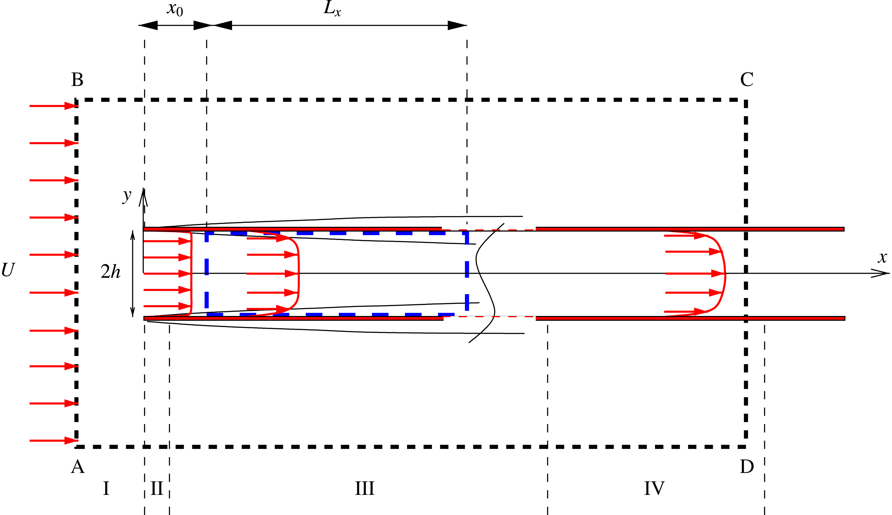
This paper is concerned with the stability properties of streaks embedded in a region near the entrance of a plane channel subjected to uniform flow conditions. Since it is not amenable to exact analytical solution, the channel entrance flow problem has motivated a wide variety of approximation methods. One source of complexity is the choice of upstream conditions. Uniform flow conditions are generally considered, with the two mostly used variants being: the condition of parallel and uniform flow, and the condition of zero vorticity. Another choice consists of specifying conditions at infinity upstream: the infinite cascade model, and the case of a single channel forming an inlet in an otherwise uniform flow. These models have been discussed within the framework of a matched series expansion (Van Dyke Reference Van Dyke1970; Wilson Reference Wilson1971; Kapila, Ludford & Olunloyo Reference Kapila, Ludford and Olunloyo1972) and by numerical simulation (Darbandi & Schneider Reference Darbandi and Schneider1999). Non-uniform upstream flows have been considered in the form of a sink flow by Sparrow & Anderson (Reference Sparrow and Anderson1977) or a Jeffrey–Hamel flow by Sadri & Floryan (Reference Sadri and Floryan2002). In the present study, a single channel is considered where uniform flow conditions are fixed far upstream of the inlet (see figure 1). In the following, the variables will be made dimensionless with the channel half-width
 $h$
and the flow-rate velocity
 $U_{0}$
across the channel inlet section; the Reynolds number is defined by
 $Re=U_{0}h/\unicode[STIX]{x1D708}$
, where
 $\unicode[STIX]{x1D708}$
is the kinematic viscosity. Using the Cartesian coordinate system
 $(x,y,z)$
, the channel walls are the two semi-infinite planes
 $y=\pm 1$
with
 $x\geqslant 0$
and the inlet section is at
 $x=0$
. We note, hereafter, the dimensionless centreline velocity
 $U_{c}$
. We recall that, for the Poiseuille flow,
 $U_{c}=1.5$
when considering the bulk velocity as the reference scale. Channel entrance flows at sufficiently high
 $Re$
are generally divided into different regions (I, II, III and IV in figure 1). Region I covers the area upstream of the leading edges of the channel. Region II concerns the area immediately adjacent downstream of the channel inlet. Region III involves accelerated boundary layers separated by an inviscid core (where velocity is uniform in the cross-section). Finally, region IV is associated with a slow deviation from the Poiseuille flow solution. This zone exhibits a universal character independent of the upstream flow conditions (see Asai & Floryan Reference Asai and Floryan2004). We are especially interested in the region III.
Sketch of the flow configuration and coordinate system. The computational box used to compute the solution into the fringe zone is shown in thick black dashed lines (delimited by points A, B, C and D). The computational box considered for global linear optimizations and DNS is depicted in thick blue dashed lines. The region upstream of the channel inlet is referenced as I. The downstream region near the inlet is marked II. Region III consists of two flat-plate accelerated boundary layers. The downstream region IV is characterized by a slow deviation from the Poiseuille flow.

The flow satisfies the incompressible Navier–Stokes equations:
 $$\begin{eqnarray}\left.\begin{array}{@{}c@{}}\displaystyle \frac{\unicode[STIX]{x2202}\boldsymbol{u}}{\unicode[STIX]{x2202}t}+(\boldsymbol{u}\boldsymbol{\cdot }\unicode[STIX]{x1D735})\boldsymbol{u}=-\unicode[STIX]{x1D735}p+\frac{1}{Re}\unicode[STIX]{x1D6FB}^{2}\boldsymbol{u},\\ \unicode[STIX]{x1D735}\boldsymbol{\cdot }\boldsymbol{u}=0,\end{array}\right\}\end{eqnarray}$$
and
 $(u,v,w)$
will denote the Cartesian components of the velocity
 $\boldsymbol{u}$
. The base flow under study is specified by the velocity field
 $\boldsymbol{U}$
, which is a steady solution of (2.1). This field splits into two parts:
 $\boldsymbol{U}=\boldsymbol{U}_{2D}+\boldsymbol{u}_{S}$
. The first part
 $\boldsymbol{U}_{2D}$
(referred to as the primary base flow, hereafter) is the two-dimensional steady solution of (2.1). The second part
 $\boldsymbol{u}_{S}$
is a disturbance that takes the form of a three-dimensional streamwise vortices/streak pattern. The disturbance, referred to as the primary disturbance, is such that
 $\boldsymbol{U}$
satisfies (2.1) without a linearization assumption at this stage. Our interest is in the space–time evolution of secondary perturbations
 $\boldsymbol{u}^{\prime }$
superimposed onto
 $\boldsymbol{U}$
. Depending on whether we are interested in purely linear effects or in the nonlinear regime, this evolution will be determined using the linearized version of (2.1) or its fully nonlinear form. The governing equations associated with the linear dynamics of
 $\boldsymbol{u}^{\prime }$
are found by substituting
 $\boldsymbol{u}=\boldsymbol{U}+\unicode[STIX]{x1D700}\boldsymbol{u}^{\prime }$
and
 $p=P+\unicode[STIX]{x1D700}p^{\prime }$
(
 $p^{\prime }$
is the pressure perturbation) into (2.1) and keeping only the first order in
 $\unicode[STIX]{x1D700}$
. It yields the following system:
 $$\begin{eqnarray}\left.\begin{array}{@{}c@{}}\displaystyle \frac{\unicode[STIX]{x2202}\boldsymbol{u}^{\prime }}{\unicode[STIX]{x2202}t}=-(\boldsymbol{U}\boldsymbol{\cdot }\unicode[STIX]{x1D735})\boldsymbol{u}^{\prime }-(\boldsymbol{u}^{\prime }\boldsymbol{\cdot }\unicode[STIX]{x1D735})\boldsymbol{U}-\unicode[STIX]{x1D735}p^{\prime }+\frac{1}{Re}\unicode[STIX]{x1D6FB}^{2}\boldsymbol{u}^{\prime },\\ \unicode[STIX]{x1D735}\boldsymbol{\cdot }\boldsymbol{u}^{\prime }=0,\end{array}\right\}\end{eqnarray}$$
which is complemented by appropriate boundary and initial conditions.
2.2 Numerical methods
The numerical method is based on a spectral Galerkin approximation of the velocity fields using Fourier expansions in both the streamwise and spanwise directions and Chebyshev polynomials in the wall-normal direction. Using a divergence-free basis set of vectors, continuity is satisfied implicitly (Moser, Moin & Leonard Reference Moser, Moin and Leonard1983) and the pressure disappears from the discretized equation. To overcome the inherent difficulties when using Fourier modes along
 $x$
, which is a direction of evolution for the flow, a fringe region technique is employed (Bertolotti, Herbert & Spalart Reference Bertolotti, Herbert and Spalart1992). By adding a forcing term into the Navier–Stokes equations, the outgoing flow is smoothly driven to the prescribed inlet condition. In order to build the target velocity field that is used in the fringe region, a preliminary calculation of the primary base flow is carried out using a second-order finite difference code (see Nordstrom, Nordin & Henningson Reference Nordstrom, Nordin and Henningson1999). The numerical method employed to compute this preliminary solution is detailed in Alizard, Robinet & Gloerfelt (Reference Alizard, Robinet and Gloerfelt2012). The streaky base flow
 $\boldsymbol{U}$
is obtained by calculating the steady solution of the governing equations when adding to the primary base flow a pair of streamwise vortices with a given amplitude, in the fringe region.
The discrete system attached to (2.1) is solved at each time step using a low-storage semi-implicit third-order Runge–Kutta scheme. Viscous terms are treated implicitly while an explicit scheme is used for the convective term, as described by Spalart, Moser & Rogers (Reference Spalart, Moser and Rogers1990). Numerical methods are further detailed in Buffat et al. (Reference Buffat, Le Penven and Cadiou2011). To solve the linearized problem (2.2), the coupling term with the base flow is also treated explicitly.
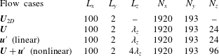
The different types of flow simulation investigated hereafter are listed in table 1, with the chosen parameters of discretization. For all flow cases, the Reynolds number is fixed to
 $Re=2500$
and the computation domain is between
 $x=x_{0}$
and
 $x=x_{0}+L_{x}$
, with
 $x_{0}=16$
and
 $L_{x}=100$
. To accurately compute the target velocity field, the preliminary solution is solved in a larger domain (see figure 1). In particular, uniform flow conditions are imposed at
 $x=-5$
while Neumann conditions are imposed at
 $y=\pm 31$
and
 $x=450$
. The grid used for this solution is clustered near walls and stretched in the streamwise direction after
 $x=0$
. The grid points are fixed to
 $N_{x}\times N_{y}=1801\times 601$
with
 $\unicode[STIX]{x0394}y=3\times 10^{-3}$
near walls. In the following, we will make use of the notation
 $x_{i}=x-x_{0}$
for the shifted streamwise coordinate. For all computations, the fringe region is located between
 $x_{i}=0.9L_{x}$
and
 $x_{i}=L_{x}$
.
Flow cases. The side lengths of the rectangular computational box are
 $L_{x}$
,
 $L_{y}$
and
 $L_{z}$
for the streamwise, wall-normal and spanwise directions, respectively;
 $N_{x}$
,
 $N_{y}$
and
 $N_{z}$
are the corresponding numbers of modes; and
 $\unicode[STIX]{x1D706}_{z}\simeq 1.14$
is the fundamental wavelength of the primary disturbance (i.e. the vortex/streak pattern).

2.3 Linear global optimization
In this section, we describe the method used to identify optimal perturbations, i.e. perturbations undergoing the largest linear growth in energy for a given time horizon. Let us first write the solution of the linearized Navier–Stokes equations around the steady state (2.2) as
 $$\begin{eqnarray}\boldsymbol{u}^{\prime }(t)={\mathcal{A}}(t)\boldsymbol{u}_{0}^{\prime }.\end{eqnarray}$$
In this form, in which the space variable is left out,
 ${\mathcal{A}}(t)$
appears as a forward time-shift operator for the initial perturbation,
 $\boldsymbol{u}^{\prime }(t=0)=\boldsymbol{u}_{0}^{\prime }\neq 0$
. It is known that streaky boundary layer flows are absolutely stable and that they can exhibit large energy growth due to convective instabilities (Brandt et al.
Reference Brandt, Cossu, Chomaz, Huerre and Henningson2003). In fact, the dynamics of interest is quantified through the singular-value decomposition of
 ${\mathcal{A}}(t)$
. We introduce the kinetic energy norm associated with the
 $L_{2}$
inner product, denoted herein as
 $\langle ~,\rangle$
, and focus on the space–time evolution of
 $\boldsymbol{u}_{0}^{\prime }$
having finite kinetic energy. The rate of change of perturbation energy is measured by
 $$\begin{eqnarray}\frac{E(t)}{E_{0}}=\frac{\langle \boldsymbol{u}^{\prime }(t),\boldsymbol{u}^{\prime }(t)\rangle }{\langle \boldsymbol{u}_{0}^{\prime },\boldsymbol{u}_{0}^{\prime }\rangle },\end{eqnarray}$$
where
 $E_{0}=E(t=0)$
. Using (2.3), we define the optimal energy growth over all possible
 $\boldsymbol{u}_{0}^{\prime }$
as
 $$\begin{eqnarray}G(t)\max _{\boldsymbol{u}_{0}^{\prime }}\frac{\langle {\mathcal{A}}^{\star }(t){\mathcal{A}}(t)\boldsymbol{u}_{0}^{\prime },\boldsymbol{u}_{0}^{\prime }\rangle }{\langle \boldsymbol{u}_{0}^{\prime },\boldsymbol{u}_{0}^{\prime }\rangle },\end{eqnarray}$$
with
 ${\mathcal{A}}^{\star }$
the adjoint operator. Thus, perturbations leading to the largest energy growth are the ones associated with the dominant eigenvalue of
 ${\mathcal{A}}^{\star }(t){\mathcal{A}}(t)$
, which is also the largest singular value of
 ${\mathcal{A}}(t)$
. An optimal perturbation at the initial time is a right-singular vector associated with the largest singular value. To determine the operator
 ${\mathcal{A}}(t)$
(or its adjoint), we follow the method developed by Barkley, Blackburn & Sherwin (Reference Barkley, Blackburn and Sherwin2008), the so-called time-stepper approach. The operator
 ${\mathcal{A}}(t)$
(or its adjoint) is first approximated by integrating forward (or backward) in time the linearized Navier–Stokes equations (or its adjoint counterpart). Then, an Arnoldi algorithm based on a Krylov subspace constructed by successive applications of
 ${\mathcal{A}}^{\star }(t){\mathcal{A}}(t)$
is used to extract the dominant singular values of
 ${\mathcal{A}}(t)$
for various time horizons. In the following, optimal disturbances of unit initial energy are referred to as optimal modes. Finally, we denote hereafter
 $G(t_{opt})$
as the dominant singular value of
 ${\mathcal{A}}(t_{opt})$
, where
 $t_{opt}$
is the target time used for the optimization.
3 Results
3.1 Primary and secondary base flows
We first consider the primary base flow
 $\boldsymbol{U}_{2D}$
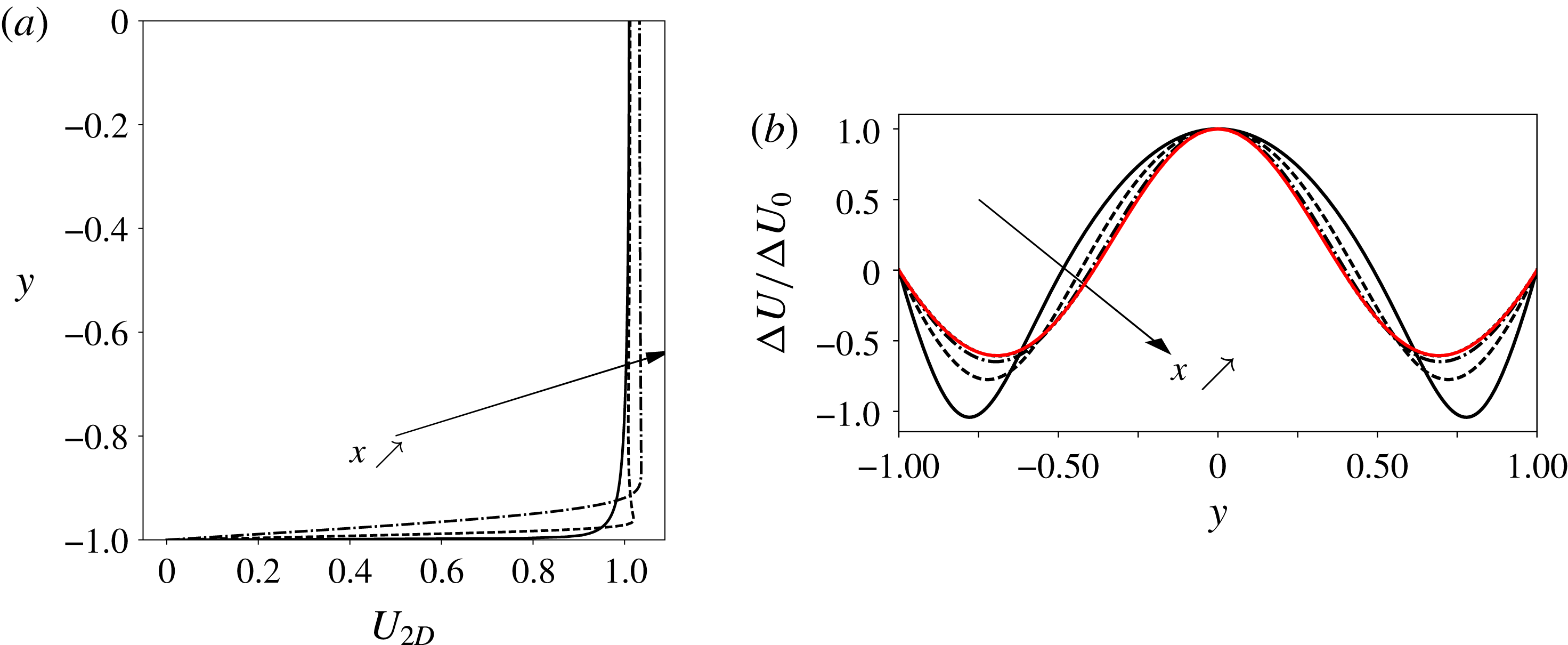
. As explained in the previous section, in order to build the target velocity field for the fringe region, a preliminary computation has been carried out on a large domain capturing the upstream influence of the leading edges of the two plates. To better characterize the domain in which laminar–turbulent transition is studied, some velocity profiles are plotted for sections close to the inlet and further downstream. In figure 2(a), we show the streamwise component of the velocity at
 $x=0$
, 0.1 and 1. While the velocity profiles have a convex shape at the inlet, for small
 $x$
, the profiles exhibit a minimum at
 $y=0$
and an overshoot in the vicinity of the wall. This effect is rapidly damped and a boundary-layer-like profile is observed for
 $x$
larger than 1.
Primary base flow
 $\boldsymbol{U}_{2D}$
. (a) Streamwise velocity profiles for
 $x=0$
, 0.1 and 1. (b) Normalized distribution of the perturbation velocity
 $\unicode[STIX]{x0394}U/\unicode[STIX]{x0394}U_{0}$
, where
 $\unicode[STIX]{x0394}U(x,y)=U_{2D}(x,y)-1.5(1-y^{2})$
and
 $\unicode[STIX]{x0394}U_{0}(x)=\unicode[STIX]{x0394}U(x,0)$
, at
 $x=20$
, 60, 120 and 200. The theoretical prediction assuming a slow deviation from the Poiseuille flow is shown in red. For
 $x=200$
, curves obtained by the model and numerical simulation are superimposed.

In the downstream zone (IV) the flow slowly evolves in the streamwise direction towards Poiseuille flow. Asai & Floryan (Reference Asai and Floryan2004) have shown that, in this region, the streamwise velocity is well approached by
 $U_{2D}(x,y)=(3/2)(1-y^{2})+A\widetilde{u}(y)\text{e}^{-kx}$
. The vanishing term corresponds to the dominant mode (i.e. the slowest modal decaying perturbation) of the linear stability problem (
 $k=(2/3)28.221$
). In figure 2(b), a close match between model prediction and numerical simulation is observed for
 $x>120$
.
In region III, the pressure gradient can be computed using the Bernoulli equation:
 $\unicode[STIX]{x2202}P/\unicode[STIX]{x2202}x|_{y=0}=-U_{c}\unicode[STIX]{x2202}U_{c}/\unicode[STIX]{x2202}x$
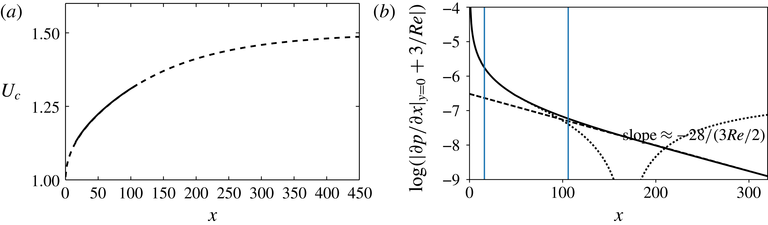
. In figure 3(a,b), we report the centreline velocity distribution
 $U_{c}$
and the streamwise pressure gradient
 $\unicode[STIX]{x2202}P/\unicode[STIX]{x2202}x|_{y=0}+3/Re$
in a logarithmic scale, respectively. In region IV, the model derived by Sadri & Floryan (Reference Sadri and Floryan2002) and Asai & Floryan (Reference Asai and Floryan2004) gives
 $\unicode[STIX]{x2202}P/\unicode[STIX]{x2202}x|_{y=0}=-3/Re+\widetilde{A}\text{e}^{-kx}$
, with
 $\widetilde{A}$
an amplitude coefficient. Figure 3(b) shows that the domain of study in the present paper is mainly associated with region III. Figure 3(a) also shows that centreline velocity distributions obtained using either the spectral code with the fringe region technique or the finite-difference code are in perfect match.
Defining the dimensionless entrance length
 $L_{e}$
as the streamwise position where
 $U_{c}$
reaches 99 % of the Poiseuille solution, there is a well-known criterion based on Blasius boundary layer argument suggesting that
 $L_{e}\sim Re$
, for large enough
 $Re$
and thus quite a large extent for the flow developing zone. The data of figure 3(a) give
 $L_{e}\approx 433$
, which is very close to the value 442 obtained with the correlation proposed by Durst et al. (Reference Durst, Ray, Ünsal and Bayoumi2005). For uniform inlet flow conditions, Darbandi & Schneider (Reference Darbandi and Schneider1999) show that, as the Reynolds number increases,
 $r=L_{e}/(4Re)$
approaches a universal value
 ${\approx}0.043$
. Here, we obtain
 $r\approx 0.0433$
. It suggests that the velocity profiles are not so sensitive to the model of uniform flow velocities.
Primary base flow
 $\boldsymbol{U}_{2D}$
. (a) Velocity at the centre of the channel: solid line, DNS code with a fringe region technique; dashed line, preliminary computation carried out with a finite-difference code of second order. (b) Streamwise evolution of the pressure gradient along the centreline,
 $\log \big|\unicode[STIX]{x2202}P/\unicode[STIX]{x2202}x|_{y=0}+3/Re\big|$
: solid line, numerical solution; dashed line, linear regression used to fit the curve; dotted line, solution based on the Bernoulli equation. Vertical lines denote streamwise positions
 $x=16$
and
 $x=106$
.

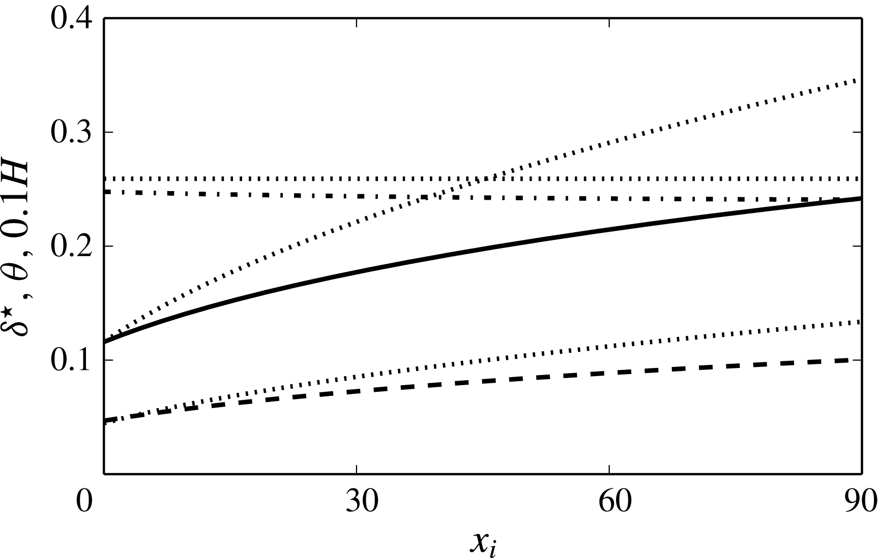
In figure 4 we show the development of the displacement and momentum thickness (
 $\unicode[STIX]{x1D6FF}^{\star }$
and
 $\unicode[STIX]{x1D703}$
, respectively) and the shape factor (i.e.
 $H=\unicode[STIX]{x1D6FF}^{\star }/\unicode[STIX]{x1D703}$
), together with the well-known values for a zero-pressure-gradient flat-plate boundary layer. Owing to the favourable pressure gradient, the boundary layers developing along the walls thicken slower than in the flat-plate case.
Primary base flow
 $\boldsymbol{U}_{2D}$
. Integral boundary layer parameters: thick solid line, displacement thickness
 $\unicode[STIX]{x1D6FF}^{\star }$
; thick dashed line, momentum thickness
 $\unicode[STIX]{x1D703}$
; thick dot-dashed line, shape factor
 $H$
; dotted lines, theoretical values for laminar Blasius profile (where
 $\unicode[STIX]{x1D6FF}^{\star }(x_{i}=0)$
is fixed equal to the entrance channel flow value).

Let us now consider the secondary base flow
 $\boldsymbol{U}$
. To generate streamwise-elongated streaks, a pair of streamwise vortices is injected in the section
 $x_{i}=0$
of the boundary layer developing along the lower wall. The shape of the perturbation is obtained by using a local, linear transient growth analysis and selecting the vortex pair that maximizes energy over all times. Only one spanwise wavelength of the optimal mode (i.e. one vortex pair) is considered. Its numerical value is
 $\unicode[STIX]{x1D706}_{z}\approx 1.14$
. When rescaled by the displacement thickness at the inlet, the corresponding spanwise wavenumber
 ${\approx}0.66$
is very close to the value associated with a flat-plate boundary layer without pressure gradient (
 ${\approx}0.65$
; see Schmid & Henningson (Reference Schmid and Henningson2001) for instance). The code used to compute the optimal vortex pair is detailed in Alizard, Robinet & Filliard (Reference Alizard, Robinet and Filliard2015).
Secondary base flow
 $\boldsymbol{U}$
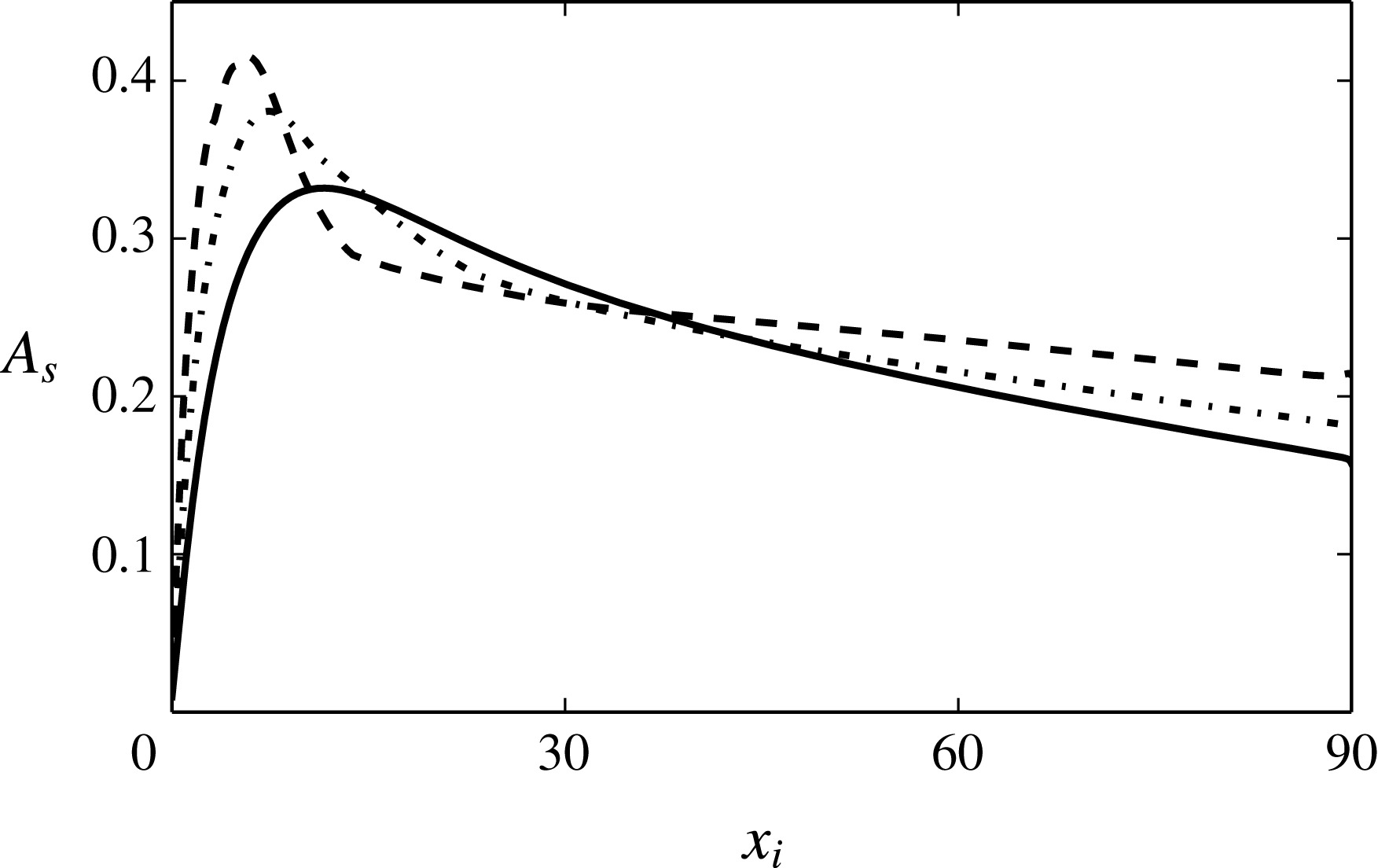
. Streamwise evolution of the streak amplitude for
 $A_{0}=0.015$
(solid),
 $A_{0}=0.025$
(dot-dashed) and
 $A_{0}=0.04$
(dashed).

Different secondary base flows are computed for different amplitudes of the vortex pair at the section
 $x_{i}=0$
. In particular, we use the kinetic energy norm to measure the amplitude of the initial streamwise vortices:
 $$\begin{eqnarray}A_{0}=\int _{-1}^{1}(v_{s}^{2}(x_{i}=0)+w_{s}^{2}(x_{i}=0))^{1/2}\,\text{d}y,\end{eqnarray}$$
with
 $v_{s}$
and
 $w_{s}$
being the normal and spanwise components of the primary disturbance. To quantify the size of the streak at each streamwise position, we define its amplitude
 $A_{s}$
as
 $$\begin{eqnarray}A_{s}(x)=\frac{1}{2U_{c}}\left[\max _{(y,z)}(U(x,y,z)-\overline{U}(x,y))-\min _{(y,z)}(U(x,y,z)-\overline{U}(x,y))\right],\end{eqnarray}$$
where
 $\overline{U}$
is the
 $z$
-average streamwise velocity and
 $U_{c}$
the mean centreline velocity,
 $U_{c}=\overline{U}(x,0)$
. The streamwise evolution of the streak amplitude is shown in figure 5 for the three increasing values
 $A_{0}=0.015$
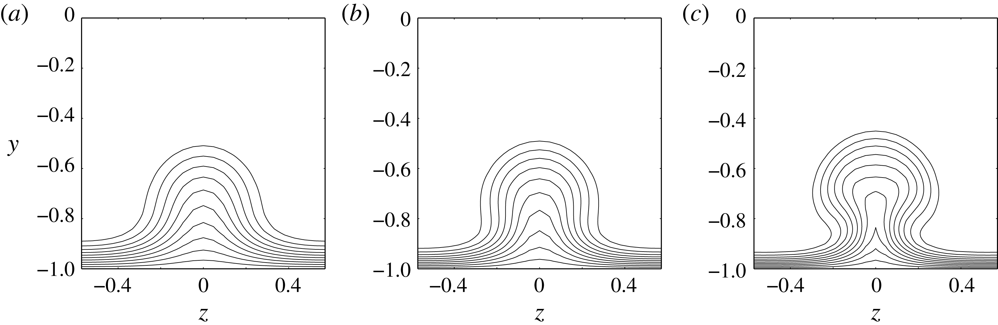
, 0.025 and 0.04. The maximum of amplitude observed during the spatial growth downstream also increases, albeit more moderately, from 0.33 to 0.42, as an effect of nonlinear saturation. While for the lowest value the streak amplitude has rather smooth variations, for the higher value, we observe that the top of the profile is strongly pinched as it shifts upstream. For all flow cases, the three-dimensional flow evolves gradually into a quasi-parallel streaky motion further downstream. In figure 6, the streak is represented for the different initial amplitudes through streamwise velocity isocontour plots in the
 $(y,z)$
section where its amplitude is maximum. As observed by several authors for the case of a flat-plate boundary layer, regions of strong spanwise shear are formed on both sides of the low-speed region, which is also displaced further away from the wall, as the initial amplitude increases. For the largest value of
 $A_{0}$
, nonlinear effects are also responsible for shaping the low-speed streak into a typical mushroom pattern.
Secondary base flow
 $\boldsymbol{U}$
. Streamwise velocity contour plot in a
 $(z,y)$
cross-stream plane at (a)
 $x_{i}=11.7$
, (b)
 $x_{i}=7.4$
and (c)
 $x_{i}=5.8$
for
 $A_{0}=0.015$
, 0.025 and 0.04, respectively.

3.2 Local exponential secondary instability
In this section, we carry out a local modal stability analysis of the secondary base flow
 $\boldsymbol{U}$
for
 $A_{0}=0.015$
, 0.025 and 0.04. For that purpose, we consider that
 $\boldsymbol{U}$
is invariant in the
 $x$
direction (i.e.
 $\boldsymbol{U}=\boldsymbol{U}(y,z)$
). A travelling wave is assumed for the secondary instability
 $\boldsymbol{u}^{\prime }$
such as
 $$\begin{eqnarray}\boldsymbol{u}^{\prime }=\hat{\boldsymbol{u}}(y,z)\text{e}^{\text{i}(\unicode[STIX]{x1D6FC}x-\unicode[STIX]{x1D714}t)}+\text{c.c.},\end{eqnarray}$$
where
 $\unicode[STIX]{x1D6FC}\in \mathbb{R}$
is the streamwise wavenumber,
 $\unicode[STIX]{x1D714}\in \mathbb{C}$
is the complex circular frequency, and c.c. denotes the complex conjugate. We decompose
 $\unicode[STIX]{x1D714}$
into a real part
 $\unicode[STIX]{x1D714}_{r}$
and an imaginary part
 $\unicode[STIX]{x1D714}_{i}$
, where the latter is the temporal amplification rate. A positive value of
 $\unicode[STIX]{x1D714}_{i}$
indicates the onset of an exponential growth mode. The linear system (2.2) reduces to an eigenvalue problem for
 $\unicode[STIX]{x1D714}$
. The code described in Alizard (Reference Alizard2015) is used to compute the least damped mode for various
 $x_{i}$
stations and
 $\unicode[STIX]{x1D6FC}$
. In addition, we restrict our analysis to sinuous and varicose modes defined as
 $$\begin{eqnarray}\hat{u} (y,z)=-\hat{u} (y,-z),\quad \hat{v}(y,z)=-\hat{v}(y,-z),\quad {\hat{w}}(y,z)={\hat{w}}(y,-z),\end{eqnarray}$$
and
 $$\begin{eqnarray}\hat{u} (y,z)=\hat{u} (y,-z),\quad \hat{v}(y,z)=\hat{v}(y,-z),\quad {\hat{w}}(y,z)=-{\hat{w}}(y,-z).\end{eqnarray}$$
respectively.
Secondary base flow
 $\boldsymbol{U}$
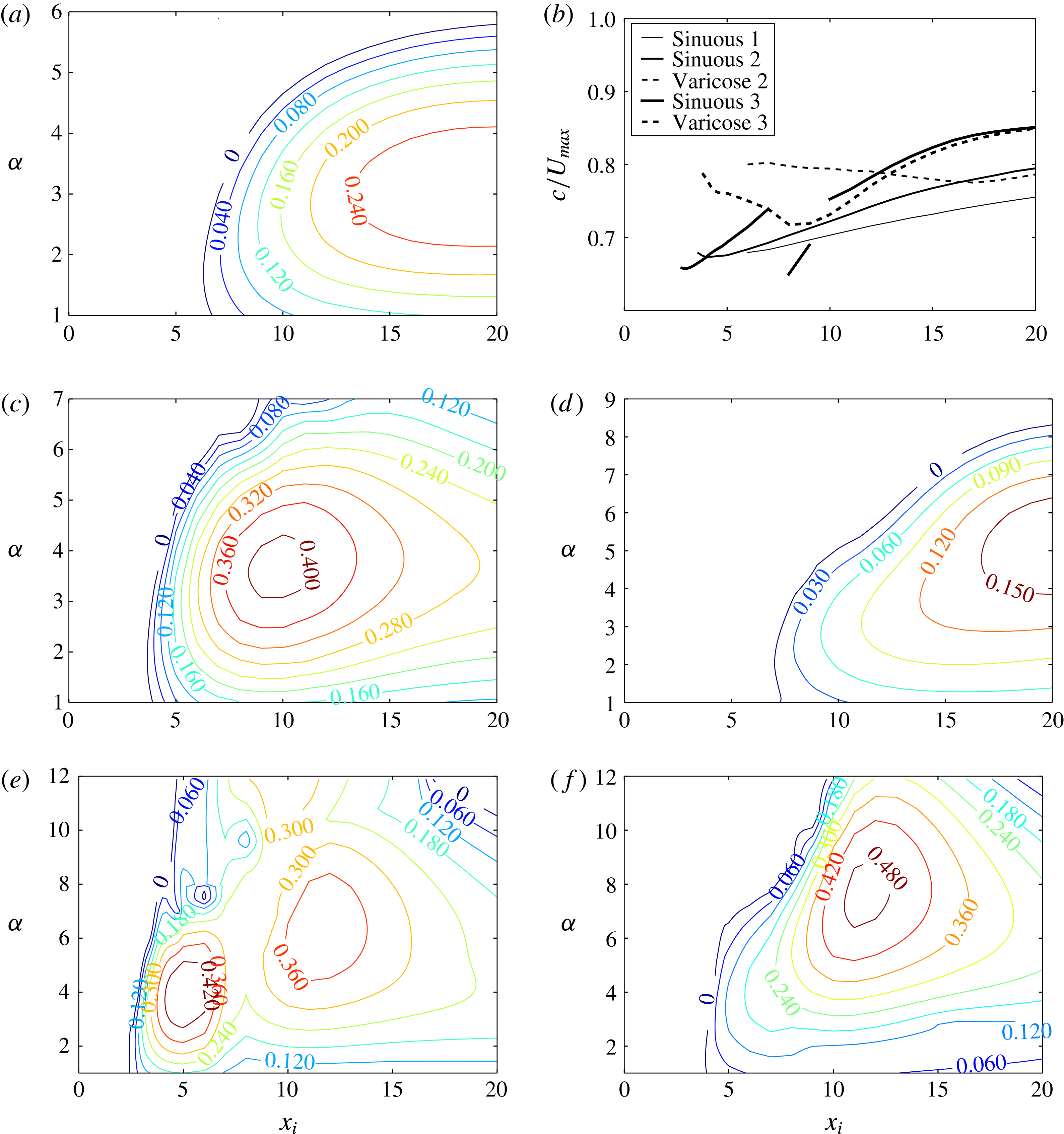
. Local stability analysis. Isocontours of the growth rate
 $\unicode[STIX]{x1D714}_{i}$
in the
 $(x_{i},\unicode[STIX]{x1D6FC})$
plane for
 $A_{0}=0.015$
(a),
 $A_{0}=0.025$
(c,d) and
 $A_{0}=0.04$
(e,f). The sinuous fundamental modes are shown in (a,c,e). The varicose fundamental modes are shown in (d,f). (b) Phase velocity
 $c=\unicode[STIX]{x1D714}_{r}/\unicode[STIX]{x1D6FC}$
made dimensionless by
 $U_{max}=\max _{y,z}U(x,y,z)$
for
 $\max \unicode[STIX]{x1D714}_{i}$
. Cases
 $A_{0}=0.015$
, 0.025 and 0.04 are referenced as 1, 2 and 3, respectively.

In figure 7, we report our results for
 $A_{0}=0.015$
, 0.025 and 0.04. For the lowest streak amplitude, figure 7(a) shows that an exponentially growing mode exists for the sinuous case when
 $x_{i}>6$
. In addition, the temporal amplification rate reaches a maximum near
 $x_{i}\approx 20$
, where
 $\unicode[STIX]{x1D714}_{i}\approx 0.28$
. For the varicose symmetry, modes are seen temporally damped. The case
 $A_{0}=0.025$
is displayed in figure 7(c,d) for the sinuous and varicose symmetries, respectively. It shows that, while the sinuous exponential mode is unstable for
 $x_{i}>3.5$
, the varicose wave is stable until
 $x_{i}\approx 7.5$
. It exhibits for all streamwise positions a lower temporal amplification rate than the sinuous mode. In particular,
 $\unicode[STIX]{x1D714}_{i}$
reaches a maximum at
 $x_{i}\approx 10$
for the sinuous mode and
 $x_{i}\approx 20$
for the varicose mode, where
 $\unicode[STIX]{x1D714}_{i}\approx 0.44$
and
 $\unicode[STIX]{x1D714}_{i}\approx 0.18$
, respectively. Results for
 $A_{0}=0.04$
are shown in figure 7(e,f). The temporal amplification rate for the sinuous symmetry exhibits two peaks at
 $x_{i}\approx 5$
and
 $x_{i}\approx 12$
, where
 $\unicode[STIX]{x1D714}_{i}\approx 0.48$
and
 $\unicode[STIX]{x1D714}_{i}\approx 0.4$
, respectively. One may remark that the onset of several modes for large streak amplitudes has also been observed recently by John, Obrist & Kleiser (Reference John, Obrist and Kleiser2016) for the leading-edge boundary layer near the attachment line. For the varicose case,
 $\unicode[STIX]{x1D714}_{i}$
peaks for
 $x_{i}\approx 12$
with a value
 ${\approx}0.5$
. While the most amplified mode has a sinuous symmetry for
 $x_{i}<8$
, it exhibits a varicose pattern for larger streamwise position. The phase velocity
 $c=\unicode[STIX]{x1D714}_{r}/\unicode[STIX]{x1D6FC}$
scaled by the maximum streamwise velocity
 $U_{max}=\max _{y,z}U$
for
 $\max _{\unicode[STIX]{x1D6FC}}\unicode[STIX]{x1D714}_{i}(\unicode[STIX]{x1D6FC},x_{i})$
is shown in figure 7(b). That panel shows that both sinuous and varicose modes propagate with a phase velocity
 $0.7<c/U_{max}<0.85$
. It is interesting to note that the onset of an exponentially growing mode is observed when
 $A_{s}\approx 30\,\%$
and
 $A_{s}\approx 38\,\%$
for the sinuous and varicose cases, respectively. These values are close to the ones computed by Andersson et al. (Reference Andersson, Brandt, Bottaro and Henningson2001) for the case of a flat-plate boundary layer (26 % and 37 %, respectively). Finally, the local stability analysis for the case
 $A_{0}=0.04$
is not able to predict which symmetry is selected by modal secondary disturbances. For the latter, temporal amplification rates reach similar values for both the varicose and sinuous case.
3.3 Global optimal perturbations: linear dynamics
3.3.1 Effect of streak amplitude and optimization time
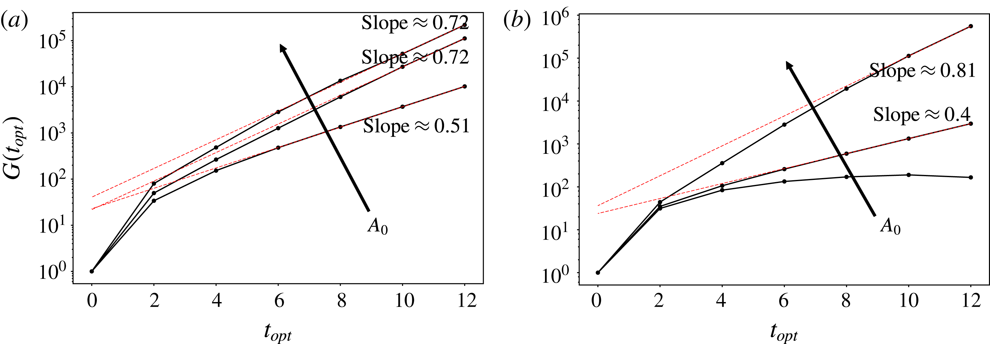
Optimizations are carried out for the secondary base flows described in the previous section. In figure 8, we report the evolution of the optimal energy gain as a function of the target time for both sinuous and varicose symmetries. For all sinuous cases, optimization curves exhibit a strong amplification between
 $t_{opt}=0$
and
 $t_{opt}=2$
and are seen to grow almost exponentially with time after that. This may suggest that optimal perturbations are subjected to a non-modal amplification for short times and behave as an exponential mode for long times. For the sinuous case, an exponential least-squares fit for
 $8<t<12$
provides exponential growth rates varying from 0.51 to 0.72 when
 $A_{0}$
is increased from 0.015 to 0.04. Recalling that
 $G(t_{opt})$
measures kinetic energy, figure 8(a) shows that optimal sinuous modes exhibit an exponential behaviour for
 $t>8$
with a temporal amplification rate
 $\unicode[STIX]{x1D70E}\approx 0.26$
for
 $A_{0}=0.015$
and
 $\unicode[STIX]{x1D70E}\approx 0.36$
for
 $A_{0}=0.025$
and 0.04. One may note a close correspondence between the amplification rates provided by the global optimization and modal local stability analysis especially for the lowest streak amplitude where non-parallelism effects are weaker (for instance,
 $\max _{(\unicode[STIX]{x1D6FC},x_{i})}\unicode[STIX]{x1D714}_{i}\approx 0.28$
for
 $A_{0}=0.015$
). For the largest streak amplitude (i.e.
 $A_{0}=0.04$
), global optimization suggests that the local instability mode corresponding to the secondary peak observed in figure 7(e) is selected for long times.
Optimal energy gain as a function of the target time for
 $A_{0}=0.015$
, 0.025 and
 $0.04$
for (a) sinuous symmetry and (b) varicose symmetry. The red dashed lines show least-squares exponential fitting for
 $8\leqslant t_{opt}\leqslant 12$
.

A similar behaviour is observed for the varicose case for
 $A_{0}=0.025$
and 0.04. Furthermore, figure 8 shows that, for
 $t_{opt}=2$
, optimal gains for varicose type reach levels of energy comparable to those of the sinuous one for all amplitudes that are considered. Figure 8 also shows that, while optimal disturbances have a sinuous symmetry for
 $A_{0}=0.015$
and 0.025, varicose configuration is the most amplified for
 $A_{0}=0.04$
. It is interesting to note that such behaviour is not well predicted by a local stability theory. In addition, for
 $A_{0}=0.015$
optimal energy gains with respect to varicose symmetry reach a maximum for
 $t_{opt}=8$
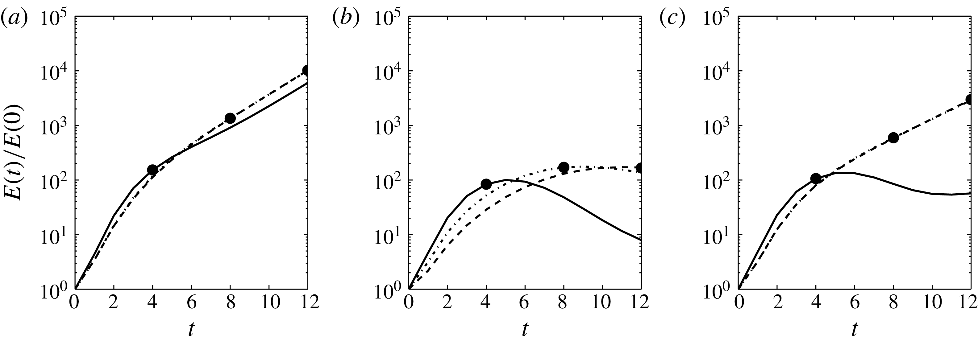
and are seen to decrease for larger time horizons. This suggests that, in this case, the varicose mode is not driven by an exponential instability. The latter remark is consistent with local stability results discussed in the previous section. For
 $t_{opt}=4$
, 8 and 12, we report time evolutions of
 $E(t)/E_{0}$
for optimal sinuous disturbances and
 $A_{0}=0.015$
in figure 9(a–c) for the varicose type, where the amplitude is fixed to
 $A_{0}=0.015$
and 0.025, respectively. For the sinuous type, kinetic energy curves exhibit an algebraic growth for short times and an almost exponential behaviour for
 $t\geqslant 8$
for all initial conditions that are considered. In particular, kinetic energy curves are superimposed for
 $t_{opt}=8$
and 12.
Kinetic energy amplification of disturbances as a function of time in the case of (a) sinuous symmetry for
 $A_{0}=0.015$
, and (b,c) varicose symmetry for
 $A_{0}=0.015$
and
 $A_{0}=0.025$
, respectively, for target times
 $t_{opt}=4$
(solid),
 $t_{opt}=8$
(dashed) and
 $t_{opt}=12$
(dot-dashed). The optimal gains associated with
 $t_{opt}=4$
, 8 and 12 are also indicated by filled circles.

In order to visualize the streamwise position of the optimal perturbations, we introduce a measure of the kinetic energy in the transverse sections:
 $$\begin{eqnarray}E_{x}(x_{i},t)=\int _{L_{y}}\int _{L_{z}}(\boldsymbol{u}^{\prime }\boldsymbol{\cdot }\boldsymbol{u}^{\prime })(x_{i},y,z,t)\,\text{d}y\,\text{d}z.\end{eqnarray}$$
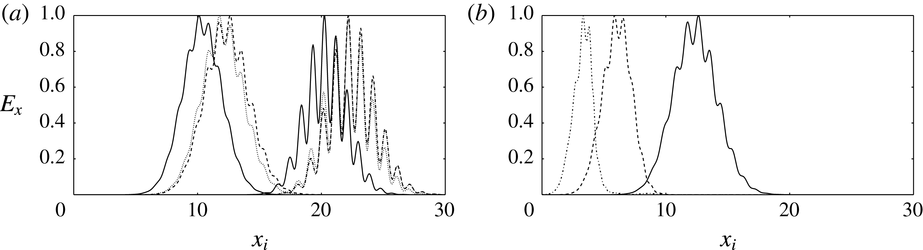
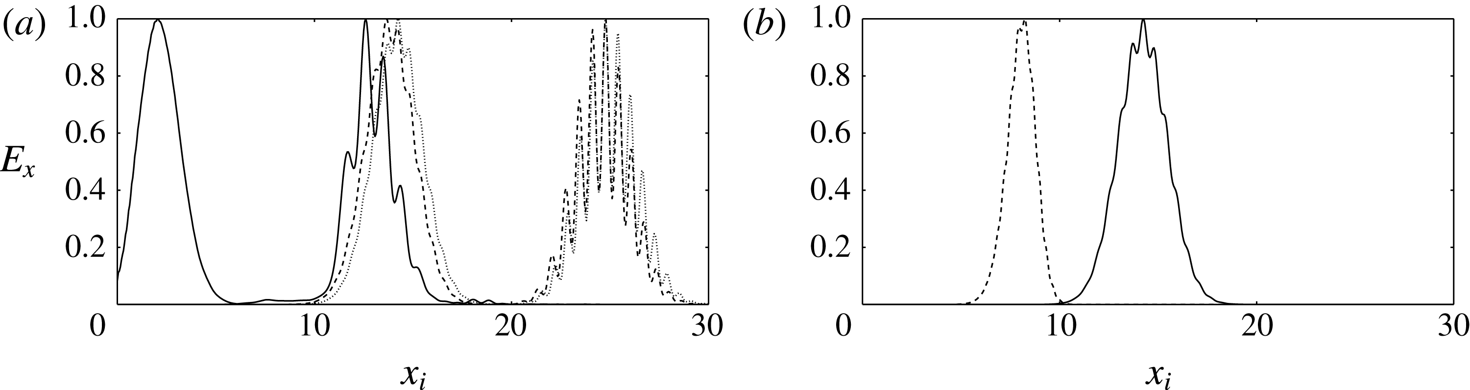
As shown in figures 10 and 11, optimal disturbances for both the varicose and sinuous cases are seen to be localized in the streamwise direction, whereas optimal modes for wall-bounded flows without streaks are dominated by infinitely elongated structures (Schmid & Henningson Reference Schmid and Henningson2001). In the case of the primary base flow for the entrance channel flow, optimal disturbances computed with a similar method yield strongly elongated streaks similar to the ones obtained by Monokrousos et al. (Reference Monokrousos, Akervik, Brandt and Henningson2010) for a flat-plate boundary layer.
Optimal sinuous and varicose modes are seen to propagate downstream as they gain kinetic energy. The latter behaviour is expected due to the convective nature of streaks as reported for the flat-plate boundary layer by Brandt et al. (Reference Brandt, Cossu, Chomaz, Huerre and Henningson2003). For the sinuous symmetry, distributions of
 $E_{x}(x_{i},t)$
for
 $t_{opt}=4$
, 8 and 12 are shown in figure 10 as a function of the distance from the inlet. For all amplitudes, figure 10 shows that for
 $t_{opt}=4$
, 8 and 12 optimal modes start to be amplified close to the streamwise position where local stability theory predicts the onset of an exponentially sinuous growing mode. Consistent with results shown in figure 9(a), the spatial support of optimal mode for
 $t_{opt}=8$
remains coincident with the one for
 $t_{opt}=12$
between
 $t=0$
and
 $t=12$
. The envelope of the optimal perturbation is seen to be unchanged for larger
 $t_{opt}$
(not shown here for the sake of conciseness). When considering the effect of
 $A_{0}$
, figure 10(b) shows that, as the streak amplitude increases, the optimal mode tends to be shifted upstream and exhibits a narrow envelope in the streamwise direction.
Sinuous case. (a) Distribution of
 $E_{x}$
as a function of the streamwise position for
 $A_{0}=0.015$
and
 $t_{opt}=4$
(solid),
 $t_{opt}=8$
(dashed) and
 $t_{opt}=12$
(dotted) at
 $t=0$
and
 $t=12$
. (b) Distribution of
 $E_{x}$
for the optimal perturbation as a function of the streamwise position for
 $t_{opt}=12$
and
 $A_{0}=0.015$
(solid),
 $A_{0}=0.025$
(dashed) and
 $A_{0}=0.04$
(dotted) at
 $t=0$
. Kinetic energy
 $E_{x}$
is normalized by its maximum for all cases.

For the varicose symmetry, when
 $A_{0}=0.015$
an algebraic growth dominates for all times. In particular, the distribution of optimal energy gain as a function of the target time exhibits a non-monotonic character (see figure 8
b). For a large optimization time (
 $t_{opt}>10$
) the optimal kinetic energy gain tends to decrease. This behaviour is also displayed by the kinetic energy curves in figure 9(b). It is consistent with the results of the local stability analysis indicating that the flow is linearly stable at all streamwise positions.
Varicose case. (a) Distribution of
 $E_{x}$
as a function of the streamwise position for
 $A_{0}=0.025$
and
 $t_{opt}=4$
(solid),
 $t_{opt}=8$
(dashed) and
 $t_{opt}=12$
(dotted) at
 $t=0$
and
 $t=12$
. (b) Distribution of
 $E_{x}$
for the optimal mode as a function of the streamwise position for
 $t_{opt}=12$
and
 $A_{0}=0.025$
(solid) and
 $A_{0}=0.04$
(dashed) at
 $t=0$
. Kinetic energy
 $E_{x}$
is normalized by its maximum for all cases.

When the amplitude is increased up to
 $A_{0}=0.025$
, we observe that the growth is due to a transient mechanism for short optimization times. In particular, the kinetic energy curve for
 $t_{opt}=4$
(and also below) exhibits a bump, whereas for
 $t_{opt}=8$
and 12 (and also above), the increase in kinetic energy is due to the combined effect of an algebraic short time mechanism and a quasi-exponential growth (see figure 9
c). This can be explained by the fact that the spatial distributions of the latter optimal modes are located in different regions. As shown in figure 11, while the optimal mode that maximizes kinetic energy for
 $t_{opt}=4$
is located in the upper part of the streaky base flow at the initial time, the one associated with
 $t_{opt}=12$
is located far downstream. In particular, at the initial time, the optimal mode for
 $t_{opt}\geqslant 6$
exhibits a spatial distribution mainly concentrated upon the streamwise position where local stability theory predicts the onset of an unstable exponential varicose mode, whereas the optimal mode for
 $t_{opt}\leqslant 4$
gets amplified in a convectively stable region.
For sinuous cases,
 $E_{x}(x_{i},t)$
is not too affected by time optimization as shown in figure 10. A similar behaviour is also observed for
 $A_{0}=0.04$
(not shown here).
Hereafter, we will consider representative varicose and sinuous perturbations that are defined such as:
(i)
 $V_{11}$
– varicose optimal mode,
$t_{opt}=2$
and
$A_{0}=0.015$
;
(ii)
$V_{12}$
– varicose optimal mode,
$t_{opt}=2$
and
$A_{0}=0.025$
;(iii)
$V_{22}$
– varicose optimal mode,
$t_{opt}=12$
and
$A_{0}=0.025$
;(iv)
$S$
– sinuous optimal mode,
$t_{opt}=12$
and
$A_{0}=0.025$
.


 $V_{11}$
,
 $V_{12}$
and
 $V_{22}$
are associated with mostly amplified varicose perturbations for short and large optimization times, respectively. Considering the weaker effect of
 $t_{opt}$
on the sinuous case, only a single mode is considered for
 $A_{0}=0.025$
, denoted
 $S$
.
3.3.2 Linear space–time dynamics and amplification mechanisms
In this section, we analyse the linear space–time dynamics for optimal wavepackets associated with varicose and sinuous symmetries. To this end, we consider two varicose modes, obtained for
 $A_{0}=0.025$
,
 $t_{opt}=2$
and
 $t_{opt}=12$
(i.e.
 $V_{12}$
and
 $V_{22}$
, respectively), and the sinuous optimal mode for the same amplitude and the target time
 $t_{opt}=12$
(denoted as
 $S$
). Let us first investigate the
 $V_{12}$
case. In figure 12, we show the streamwise and the spanwise components of vorticity and the streamwise component of velocity of the perturbation for times
 $t=0$
,
 $t=1$
and
 $t=3$
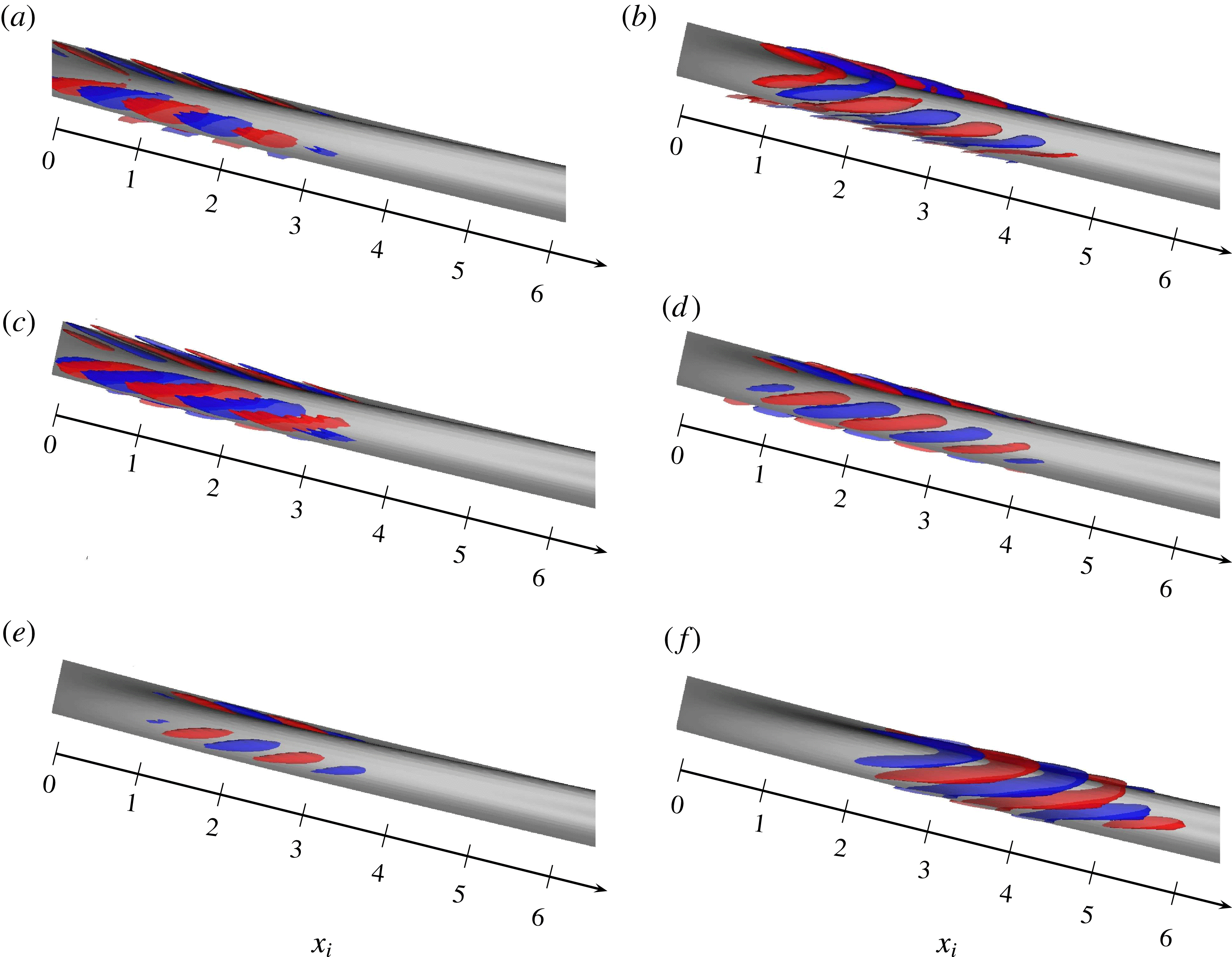
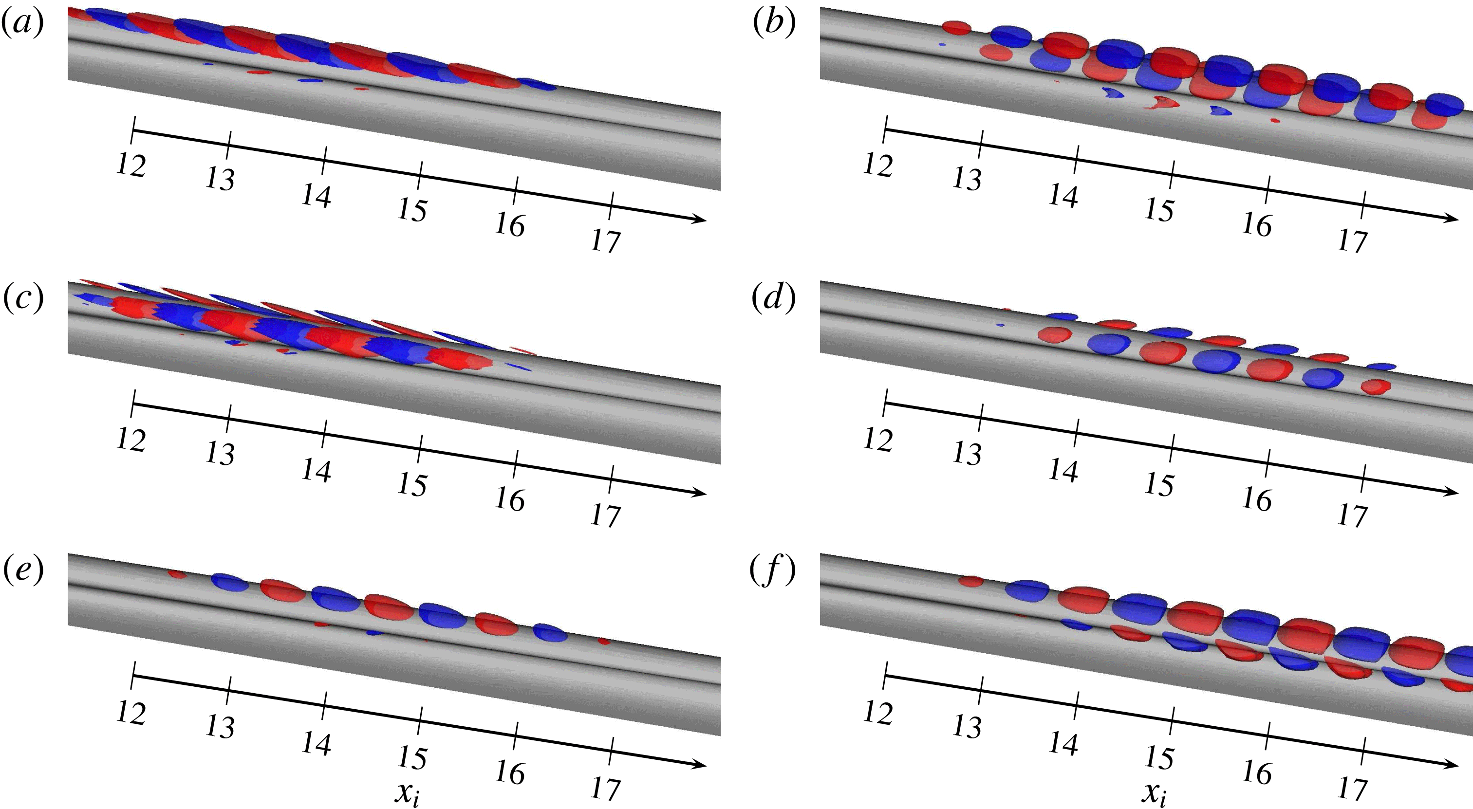
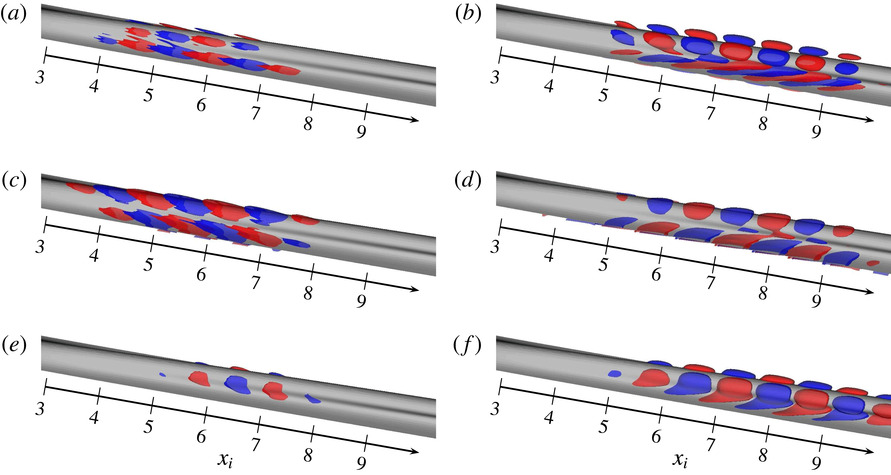
. The optimal mode takes the form of a wavepacket localized upstream at the initial time. For such a time, the perturbation is inclined in the upstream direction and is composed of both wall-normal and spanwise vorticity components, mainly localized in the flanks of the low-speed streak. Then, as time evolves, the mode is reoriented along the wall-normal shear direction where the streamwise component gets amplified and is elongated in the streamwise direction. For the times shown in figure 12, the wavepacket is localized in a region where local stability theory predicts that exponential modes are stable. From the above discussion, figure 12 suggests a combined effect due to Orr and lift-up mechanisms for the growth of initial disturbances.
Varicose case
 $V_{12}$
. The
 $L_{2}$
norm of the perturbation is fixed equal to unity at
 $t=0$
. Isosurfaces of spanwise and streamwise perturbation vorticity components are shown in (a,b) and (c,d), respectively, for times
 $t=0$
(a,c) and
 $t=1$
(b,d). Surface levels correspond to
 $\pm 500$
. Isosurfaces of the streamwise perturbation velocity component are shown in (e,f) for
 $t=1$
and
 $t=3$
. Surface levels correspond to
 $\pm 100$
. The surface level 0.7 for the streamwise component of the base flow is represented in grey for all panels.

To gain further insight into these amplification mechanisms, we analyse hereafter the different terms involved in the time evolution of the integrated kinetic energy of disturbances. For that purpose, we introduce the so-called Reynolds–Orr equation,
 $$\begin{eqnarray}\frac{\text{d}E}{\text{d}t}=-\!\int _{D}(\boldsymbol{u}^{\prime }\boldsymbol{\cdot }\unicode[STIX]{x1D735}\boldsymbol{U})\boldsymbol{\cdot }\boldsymbol{u}^{\prime }\,\text{d}D-\frac{1}{Re}\int _{D}\unicode[STIX]{x1D735}\boldsymbol{u}^{\prime }\boldsymbol{ : }\unicode[STIX]{x1D735}\boldsymbol{u}^{\prime }\,\text{d}D,\end{eqnarray}$$
where
 $\boldsymbol{ : }$
represents the double dot product operator and
 $D$
the computational box. The first term on the right-hand side is a production term associated with interactions with the mean shear and the second term is the dissipation due to viscous effects (denoted
 ${\mathcal{D}}$
, hereafter), respectively. In particular, we denote by
 $T_{y}=-\!\int _{D}u^{\prime }v^{\prime }\,\unicode[STIX]{x2202}U/\unicode[STIX]{x2202}y\,\text{d}D$
and
 $T_{z}=-\!\int _{D}u^{\prime }w^{\prime }\,\unicode[STIX]{x2202}U/\unicode[STIX]{x2202}z\,\text{d}D$
the production terms associated with the work of the Reynolds stresses against the wall-normal shear
 $\displaystyle \unicode[STIX]{x2202}U/\unicode[STIX]{x2202}y$
and the spanwise shear
 $\displaystyle \unicode[STIX]{x2202}U/\unicode[STIX]{x2202}z$
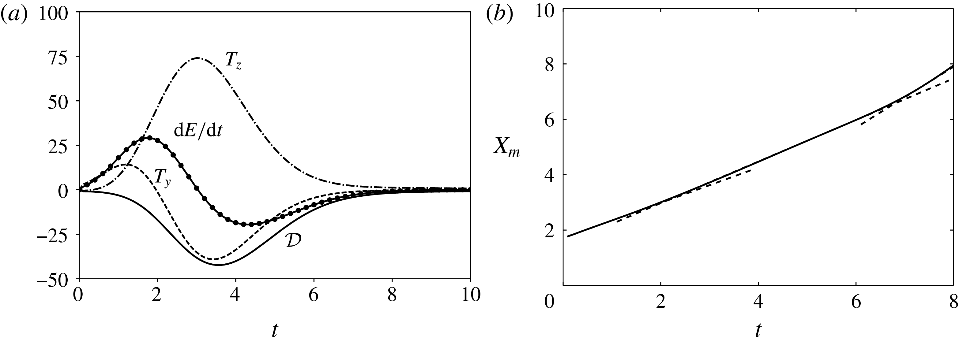
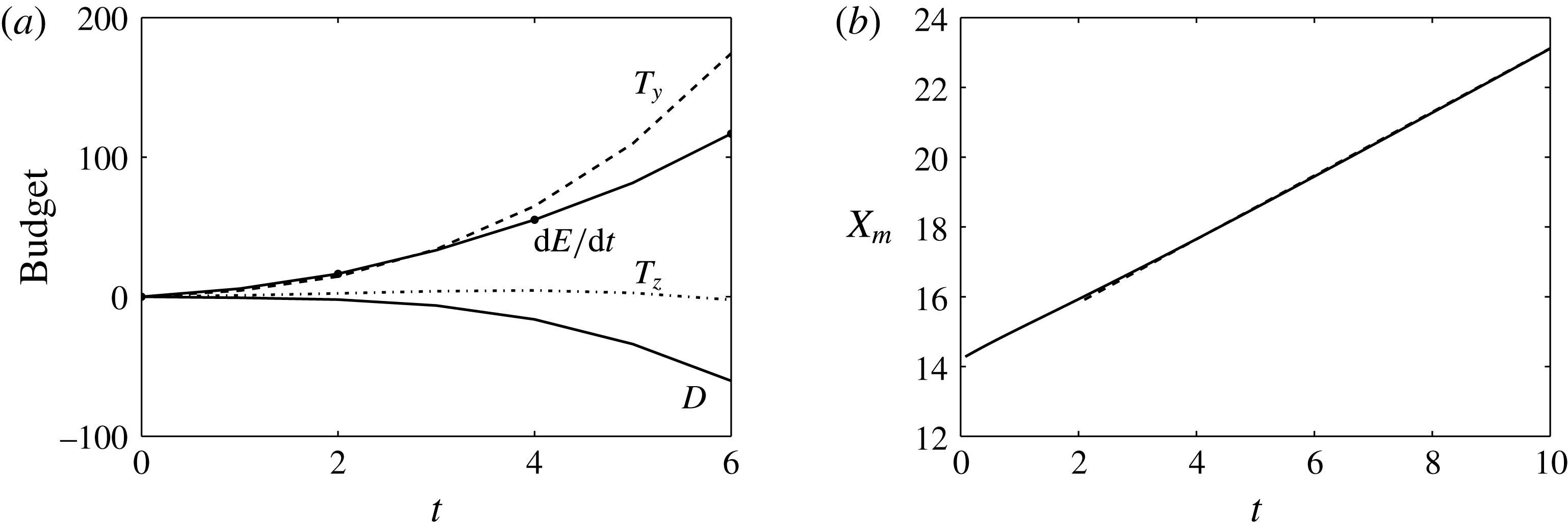
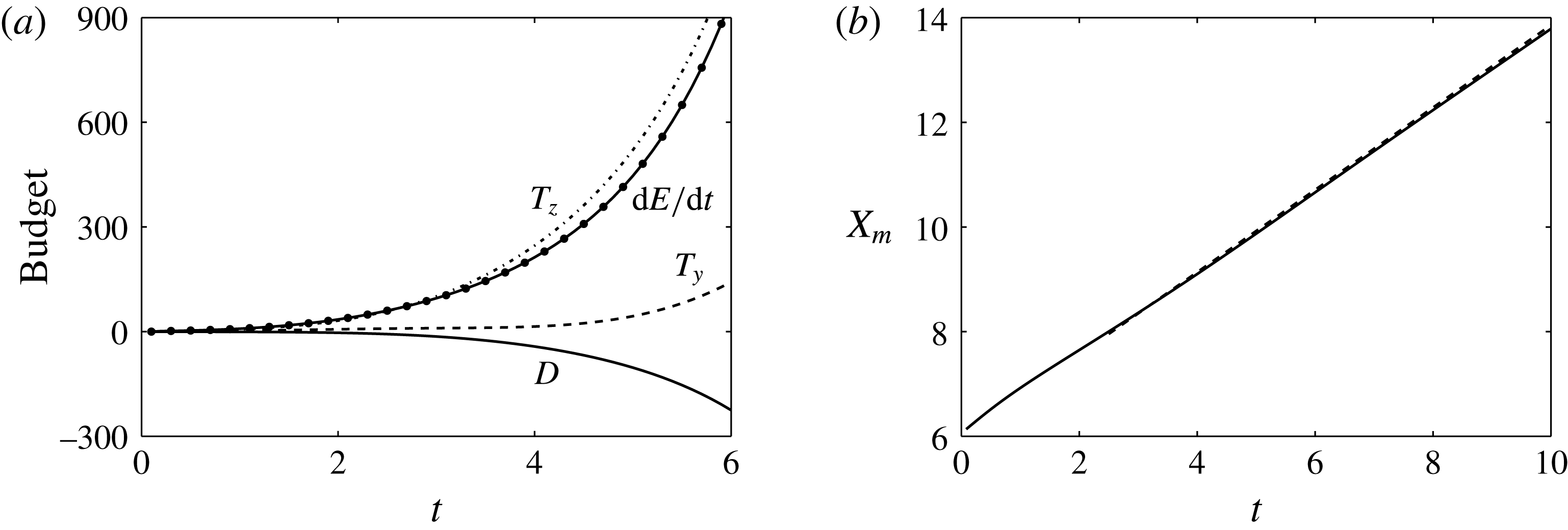
, respectively. The time evolution of the contributions to the kinetic energy budget is reported in figure 13(a). We also report in figure 13(b) the time evolution of the wavepacket barycentre defined as
 $$\begin{eqnarray}X_{m}(t)=\int _{L_{x}}xE_{x}(x,t)\,\text{d}x\left[\int _{L_{x}}E_{x}(x,t)\,\text{d}x\right]^{-1}.\end{eqnarray}$$
Figure 13(a) shows that production terms
 $T_{y}$
and
 $T_{z}$
contribute mainly to the growth; the other ones can thus be considered as negligible. As reported in figure 13(b), the wavepacket is concentrated near the inlet, above the onset of a varicose exponentially growing mode, and propagates with a low velocity
 ${\approx}0.6U_{c}$
for
 $t<4$
. This velocity is substantially lower than the speed of modal secondary varicose instability given by local stability analysis carried out in § 3.2. We may also remark that the wavepacket is localized in a region where the base flow varies significantly along the streamwise direction (see figure 5). The production term associated with the wall-normal shear of the basic flow is positive until
 $t=2$
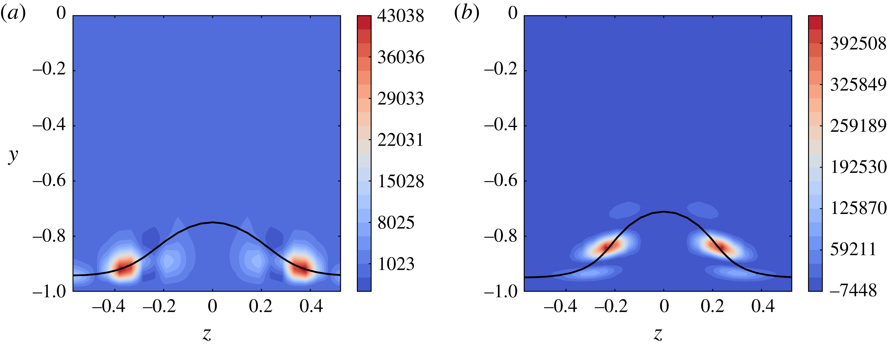
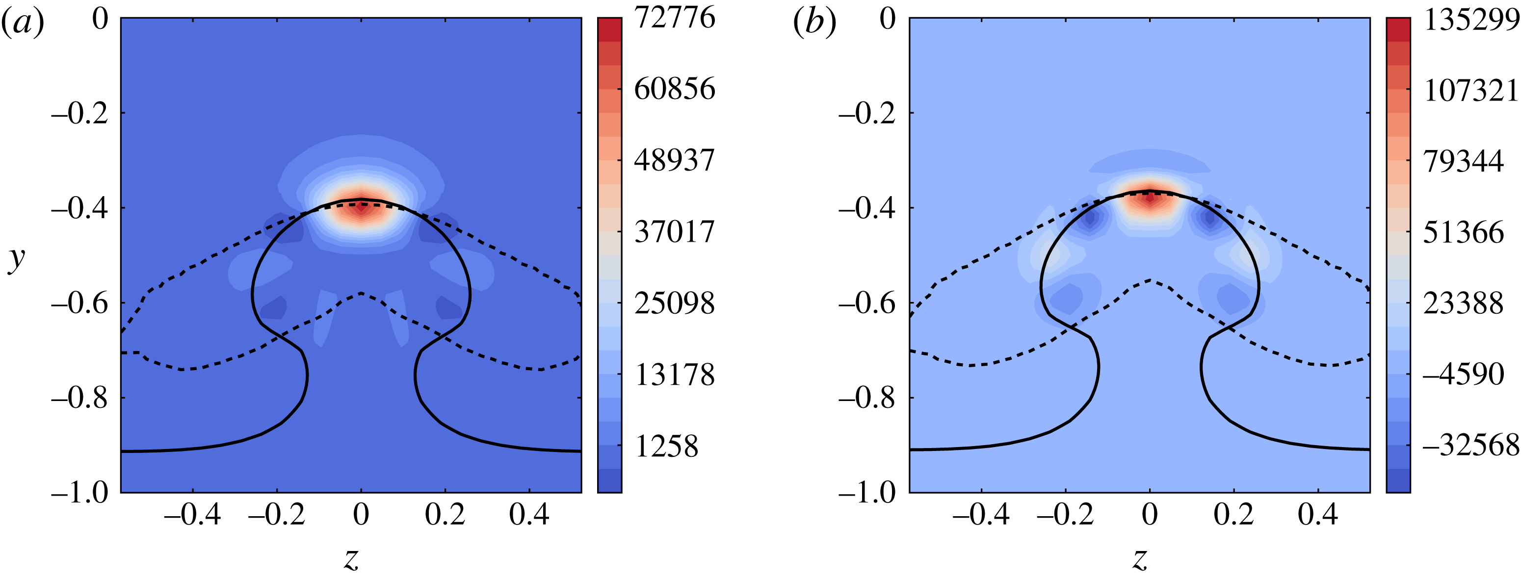
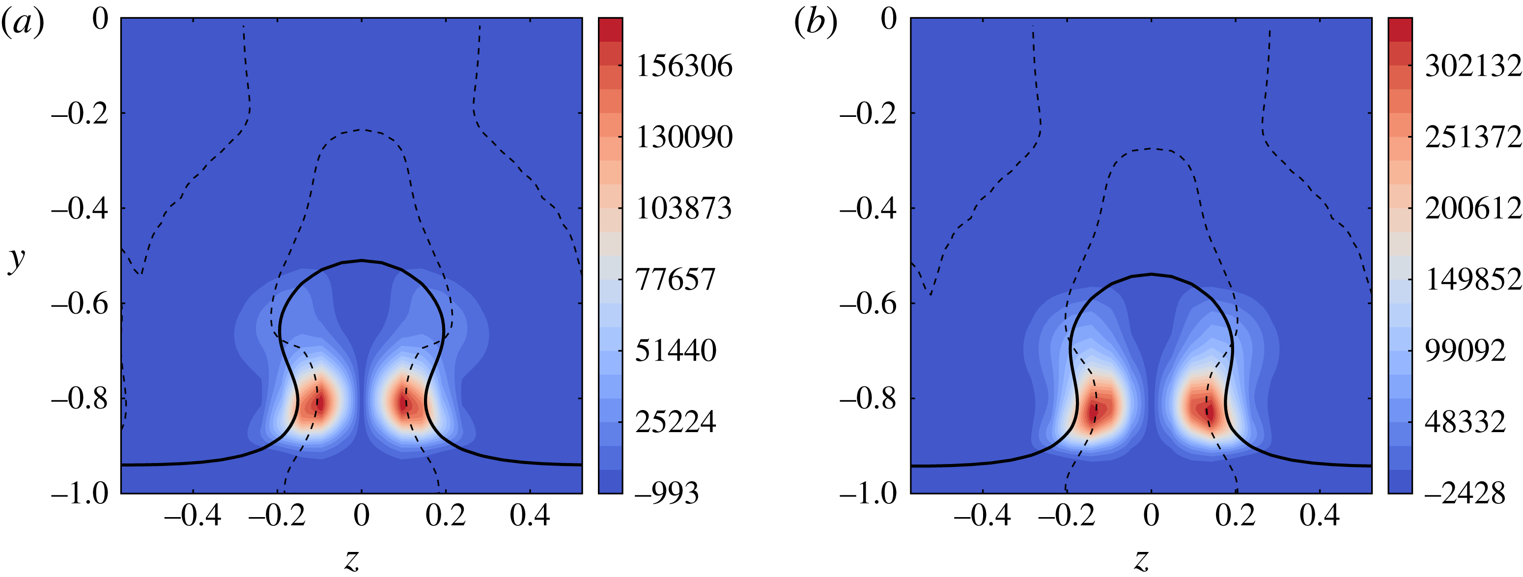
and then becomes negative. We also note that the production term that corresponds to the work of the Reynolds stress against the spanwise shear is dominant for times greater than 1. This is somewhat unexpected, since it is well accepted that varicose perturbations are driven by the action of the wall-normal basic shear (see Cossu & Brandt (Reference Cossu and Brandt2004) for instance). Such a behaviour was also observed by Hoepffner et al. (Reference Hoepffner, Brandt and Henningson2005) using a local optimal mode analysis for a streaky boundary layer flow and by Cherubini et al. (Reference Cherubini, De Tullio, De Palma and Pascazio2013) for a flow behind a roughness element using a global optimal mode theory. In figure 14, we show cross-sections of
 $T_{y}$
and
 $T_{z}$
at
 $t=1.2$
and
 $t=3$
, respectively, where production terms peak. The streamwise positions of extracted planes are fixed to the barycentre position for these times. From figure 14, we may observe that production terms (both
 $T_{y}$
and
 $T_{z}$
) are mainly localized on the flanks of the low-speed streak, which is consistent with the spatial distribution of the optimal mode shown in figure 12.
Varicose case
 $V_{12}$
. (a) Time evolution of the kinetic energy budget. (b) Time evolution of the barycentre position. The dashed lines show a linear regression used to fit the curve for three space intervals. The three slope values are 0.63, 0.75 and 1.1.

Varicose case
 $V_{12}$
. Cross-sections of production terms (a)
 $T_{y}$
at
 $t=1.2$
for
 $x_{i}=X_{m}(t=1.2)\approx 2.7$
and (b)
 $T_{z}$
at
 $t=3$
for
 $x_{i}=X_{m}(t=3)\approx 3.7$
. The full line represents the position where
 $U=0.7$
.

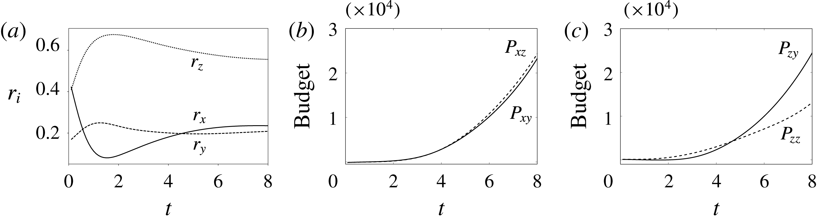
Varicose case
 $V_{12}$
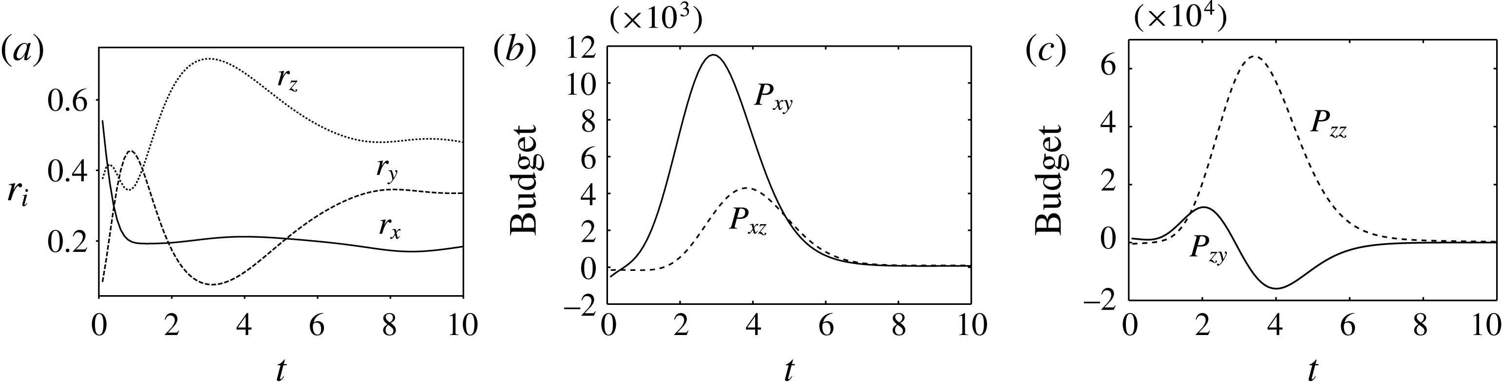
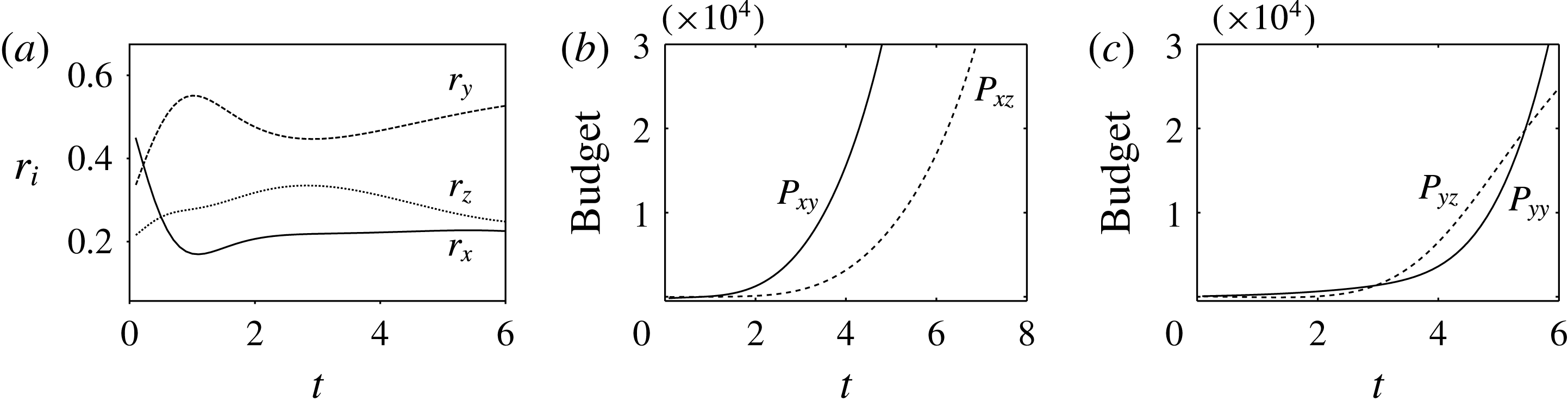
. (a) Time evolution of
 $r_{x}$
,
 $r_{y}$
and
 $r_{z}$
. Vorticity budget for
 $\unicode[STIX]{x1D6FA}_{x}^{\prime }$
(b) and
 $\unicode[STIX]{x1D6FA}_{z}^{\prime }$
(c).

To get a better understanding of the underlying mechanisms, we investigate the time evolution of the enstrophy ratios, defined as
 $$\begin{eqnarray}\displaystyle r_{i}={\displaystyle \frac{\unicode[STIX]{x1D6FA}_{i}^{\prime }}{\displaystyle \mathop{\sum }_{j}\unicode[STIX]{x1D6FA}_{j}^{\prime }}}\quad \text{with }\displaystyle \unicode[STIX]{x1D6FA}_{i}^{\prime }=\int _{D}{\unicode[STIX]{x1D74E}_{i}^{\prime }}^{2}\,\text{d}D\text{ and for }i=x,y,z,\end{eqnarray}$$
where
 $\unicode[STIX]{x1D74E}^{\prime }=\unicode[STIX]{x1D735}\times \boldsymbol{u}^{\prime }$
is the perturbation vorticity vector. A similar analysis was conducted by Schmidt et al. (Reference Schmidt, Hosseini, Rist, Hanifi and Henningson2015) to understand the physical mechanisms associated with optimal wavepackets growing in a corner flow. At the initial time, the perturbation is mainly composed of spanwise and streamwise vorticity components as shown in figure 15(a). For early times, we observe an increase in the contribution of the wall-normal vorticity component. In addition, the spanwise vorticity contribution remains almost constant during this stage, which is associated with the Orr mechanism observed in figure 14. For
 $t>1$
, a strong increase of the spanwise vorticity contribution is observed. While the increase of
 $r_{y}$
may be attributed to a lift-up mechanism whereby vorticity is transferred from the streamwise to the wall-normal direction, the understanding of
 $r_{z}$
increasing requires further analysis. To this end, we introduce the transport equations of the three components of the vorticity perturbation:
 $$\begin{eqnarray}\displaystyle & \displaystyle \frac{\text{d}\unicode[STIX]{x1D714}_{x}^{\prime }}{\text{d}t}\approx \frac{\unicode[STIX]{x2202}U}{\unicode[STIX]{x2202}z}\frac{\unicode[STIX]{x2202}v^{\prime }}{\unicode[STIX]{x2202}x}-\frac{\unicode[STIX]{x2202}U}{\unicode[STIX]{x2202}y}\frac{\unicode[STIX]{x2202}w^{\prime }}{\unicode[STIX]{x2202}x}+\frac{1}{Re}\unicode[STIX]{x0394}\unicode[STIX]{x1D714}_{x}^{\prime }, & \displaystyle\end{eqnarray}$$
 $$\begin{eqnarray}\displaystyle & \displaystyle \frac{\text{d}\unicode[STIX]{x1D714}_{y}^{\prime }}{\text{d}t}\approx \frac{\unicode[STIX]{x2202}U}{\unicode[STIX]{x2202}z}\frac{\unicode[STIX]{x2202}v^{\prime }}{\unicode[STIX]{x2202}y}-\frac{\unicode[STIX]{x2202}U}{\unicode[STIX]{x2202}y}\frac{\unicode[STIX]{x2202}v^{\prime }}{\unicode[STIX]{x2202}z}+\frac{1}{Re}\unicode[STIX]{x0394}\unicode[STIX]{x1D714}_{y}^{\prime }, & \displaystyle\end{eqnarray}$$
 $$\begin{eqnarray}\displaystyle & \displaystyle \frac{\text{d}\unicode[STIX]{x1D714}_{z}^{\prime }}{\text{d}t}\approx \frac{\unicode[STIX]{x2202}U}{\unicode[STIX]{x2202}z}\frac{\unicode[STIX]{x2202}w^{\prime }}{\unicode[STIX]{x2202}y}-\frac{\unicode[STIX]{x2202}U}{\unicode[STIX]{x2202}y}\frac{\unicode[STIX]{x2202}w^{\prime }}{\unicode[STIX]{x2202}z}+\frac{1}{Re}\unicode[STIX]{x0394}\unicode[STIX]{x1D714}_{z}^{\prime }, & \displaystyle\end{eqnarray}$$
in which we have neglected the streamwise derivative of the streamwise component of the secondary base flow velocity and the derivatives of its
 $y$
and
 $z$
components. Multiplying both sides of (3.10) by
 $\unicode[STIX]{x1D714}_{x}^{\prime }$
and integrating over the whole domain yields
 $$\begin{eqnarray}\frac{1}{2}\frac{\text{d}\unicode[STIX]{x1D6FA}_{x}^{\prime }}{\text{d}t}\approx \underbrace{\int _{D}\frac{\unicode[STIX]{x2202}U}{\unicode[STIX]{x2202}z}\frac{\unicode[STIX]{x2202}v^{\prime }}{\unicode[STIX]{x2202}x}\unicode[STIX]{x1D714}_{x}^{\prime }\,\text{d}D}_{P_{xz}}\underbrace{-\int _{D}\frac{\unicode[STIX]{x2202}U}{\unicode[STIX]{x2202}y}\frac{\unicode[STIX]{x2202}w^{\prime }}{\unicode[STIX]{x2202}x}\unicode[STIX]{x1D714}_{x}^{\prime }\,\text{d}D}_{P_{xy}}+\underbrace{\frac{1}{Re}\int _{D}\unicode[STIX]{x1D714}_{x}^{\prime }\unicode[STIX]{x0394}\unicode[STIX]{x1D714}_{x}^{\prime }\,\text{d}D}_{D_{x}},\end{eqnarray}$$
where
 $P_{xz}$
is associated with the tilting of
 $\unicode[STIX]{x2202}v^{\prime }/\unicode[STIX]{x2202}x$
by the spanwise shear and
 $P_{xy}$
is a production term due to the tilting of
 $\unicode[STIX]{x2202}w^{\prime }/\unicode[STIX]{x2202}x$
by the wall-normal shear;
 $D_{x}$
is a viscous dissipation term. For the transport of
 $\unicode[STIX]{x1D6FA}_{y}^{\prime }$
, we have
 $$\begin{eqnarray}\frac{1}{2}\frac{\text{d}\unicode[STIX]{x1D6FA}_{y}^{\prime }}{\text{d}t}\approx \underbrace{\int _{D}\frac{\unicode[STIX]{x2202}U}{\unicode[STIX]{x2202}z}\frac{\unicode[STIX]{x2202}v^{\prime }}{\unicode[STIX]{x2202}y}\unicode[STIX]{x1D714}_{y}^{\prime }\,\text{d}D}_{P_{yz}}\underbrace{-\int _{D}\frac{\unicode[STIX]{x2202}U}{\unicode[STIX]{x2202}y}\frac{\unicode[STIX]{x2202}v^{\prime }}{\unicode[STIX]{x2202}z}\unicode[STIX]{x1D714}_{y}^{\prime }\,\text{d}D}_{P_{yy}}+\underbrace{\frac{1}{Re}\int _{D}\unicode[STIX]{x1D714}_{y}^{\prime }\unicode[STIX]{x0394}\unicode[STIX]{x1D714}_{y}^{\prime }\,\text{d}D}_{D_{y}},\end{eqnarray}$$
where
 $P_{yz}$
is a vortex-stretching term due to the spanwise shear and
 $P_{yy}$
is a production term due to the tilting of
 $\unicode[STIX]{x2202}v^{\prime }/\unicode[STIX]{x2202}z$
by the wall-normal shear;
 $D_{y}$
is a viscous dissipation term. Similarly, we obtain for
 $\unicode[STIX]{x1D6FA}_{z}^{\prime }$
 $$\begin{eqnarray}\frac{1}{2}\frac{\text{d}\unicode[STIX]{x1D6FA}_{z}^{\prime }}{\text{d}t}\approx \underbrace{\int _{D}\frac{\unicode[STIX]{x2202}U}{\unicode[STIX]{x2202}z}\frac{\unicode[STIX]{x2202}w^{\prime }}{\unicode[STIX]{x2202}y}\unicode[STIX]{x1D714}_{z}^{\prime }\,\text{d}D}_{P_{zz}}\underbrace{-\int _{D}\frac{\unicode[STIX]{x2202}U}{\unicode[STIX]{x2202}y}\frac{\unicode[STIX]{x2202}w^{\prime }}{\unicode[STIX]{x2202}z}\unicode[STIX]{x1D714}_{z}^{\prime }\,\text{d}D}_{P_{zy}}+\underbrace{\frac{1}{Re}\int _{D}\unicode[STIX]{x1D714}_{z}^{\prime }\unicode[STIX]{x0394}\unicode[STIX]{x1D714}_{z}^{\prime }\,\text{d}D}_{D_{z}},\end{eqnarray}$$
where
 $P_{zz}$
is a vortex-tilting term due to the spanwise shear and
 $P_{zy}$
is a vortex-stretching production term associated with the wall-normal shear;
 $D_{z}$
is a viscous dissipation term.
Figure 15(b) shows that the transient mechanism gives rise to a positive production term for the streamwise vorticity for
 $t>1$
. The latter is mainly due to the wall-normal shear, as also found by Brandt & de Lange (Reference Brandt and de Lange2008) for the symmetric breakdown of the streak by DNS for a flat-plate boundary layer. In figure 15(c), we show
 $P_{zy}$
and
 $P_{zz}$
as a function of time. As can be seen, production terms reach a higher level than their streamwise vorticity counterparts. One may also note that for
 $t<2$
the production term is slightly dominated by
 $P_{zy}$
before being temporally damped. For larger times, figure 15(c) shows that production terms are mainly driven by
 $P_{zz}$
. While the behaviour of
 $P_{zy}$
is due to a stretching of the perturbation that rotates around the
 $z$
-axis under the action of the Orr mechanism,
 $P_{zz}$
can be associated with the lift-up mechanism due to the spanwise shear. The mean wall-normal vorticity is tilted into the
 $z$
-direction by the perturbation strain rate
 $\unicode[STIX]{x2202}w^{\prime }/\unicode[STIX]{x2202}y$
, giving rise to the increase of spanwise vorticity. It is classically admitted that for three-dimensional perturbations transient mechanisms are associated with the combined effect of an Orr and lift-up mechanism as well detailed in Butler & Farrell (Reference Butler and Farrell1992). However, the latter authors consider only a base flow with a wall-normal shear. In this case, the combined effect of Orr and lift-up mechanisms is due to both the wall-normal and spanwise shear of the base flow. Furthermore, the similarities between figures 13(a) and 15(c) give strong indications that the kinetic energy is mainly driven by the spanwise vorticity production term identified above. Finally, for times larger than 6, the flow relaxes to an equilibrium state, suggesting that the flow is driven by a modal mechanism for these times (see figure 15
a).
For
 $V_{22}$
, we report in figure 16(a–d) the spanwise and streamwise vorticity components for this mode at
 $t=0$
and
 $t=2$
. It can be seen that the optimal mode takes the form of a wavepacket that is localized downstream where local stability theory predicts the onset of a varicose exponentially growing mode (see figure 7
c). Figure 16 shows that, while
 $V_{12}$
is mostly concentrated in the flanks of the low-speed streak,
 $V_{22}$
is strongly localized on its head, as also identified through its streamwise component in figure 16(e,f). In addition,
 $V_{22}$
extends in the streamwise direction over a larger distance than
 $V_{12}$
. As for
 $V_{12}$
,
 $V_{22}$
is initially inclined against the mean shear and is reoriented along the streamwise direction while being convected downstream. Finally, one may also observe from figure 16(e,f) that the streamwise component increases significantly less with time in comparison with
 $V_{12}$
. To give further insight about the mechanisms that are responsible for the growth, we report in figure 17(a) the kinetic energy budget for
 $V_{22}$
. Figure 17(a) shows that, while both spanwise and wall-normal shear contribute to an increase in kinetic energy for
 $V_{12}$
, the production is only driven by
 $T_{y}$
for
 $V_{22}$
. In figure 17(b), we also report the time evolution of its barycentre. It shows that
 $V_{22}$
travels with a group velocity
 ${\approx}0.9U_{c}$
, which confirms that the mode is convected downstream by the outer region of the boundary layer associated with the lower wall.
Varicose case
 $V_{22}$
. The
 $L_{2}$
norm of the perturbation is fixed equal to unity at
 $t=0$
. Isosurfaces of spanwise and streamwise perturbation vorticity components are shown in (a,b) and (c,d), respectively, for times
 $t=0$
(a,c) and
 $t=1$
(b,d). Surface levels correspond to
 $\pm 500$
. Isosurfaces of the streamwise perturbation velocity component is shown in (e,f) for
 $t=1$
and
 $t=3$
. Surface levels correspond to
 $\pm 100$
. The surface level 0.8 for the streamwise component of the base flow is represented in grey for all panels.

Optimal mode
 $V_{22}$
. (a) Time evolution of kinetic energy budget. (b) Time evolution of barycentre position. The dashed line shows
 $\text{d}X_{m}/\text{d}t\approx 0.9$
.

Figure 18 displays cross-sections of the dominant production term
 $T_{y}$
for
 $t=3$
and
 $t=5$
at
 $x_{i}=X_{m}(t=3)$
and
 $x_{i}=X_{m}(t=5)$
, respectively. We also report the position of the inflection point associated with the low-speed streak and the velocity contour where
 $U=\text{d}X_{m}/\text{d}t$
. Figure 18 shows that the production term
 $T_{y}$
is mainly localized around the inflection point. This characteristic is observed for times
 $t>3$
.
Varicose case
 $V_{22}$
. Production terms
 $T_{y}$
at
 $t=3$
(a) and
 $t=5$
(b) for
 $x_{i}=X_{m}(t=3)=16.8$
and
 $x_{i}=X_{m}(t=5)=18.5$
, respectively. The full line represents the position where
 $U=\text{d}X_{m}/\text{d}t$
. Dashed lines represent positions of wall-normal inflection points.

In figure 19(a), we report the temporal evolutions of the normalized perturbation enstrophy ratios for
 $V_{22}$
. In figure 19(b,c), production terms associated with streamwise and spanwise vorticity components are displayed. Figure 19(a) shows that the initial solution predominantly consists of streamwise and spanwise vorticity. During the initial stage of transient amplification, a part of the vorticity is transferred from the streamwise to the wall-normal component. The underlying evolution is characteristic of the lift-up mechanism associated with the wall-normal shear. We also observe in figure 19(c) that a part of the streamwise vorticity is transferred to the spanwise component. During this preliminary stage, the tilting term (i.e due to the spanwise shear) is dominant. However, the contribution to the kinetic energy budget of the production associated with the spanwise shear is negligible, in contrast to its important role in the increase of kinetic energy for
 $V_{12}$
. Hence, the mechanism responsible for the growth is seen to be associated with a combination of Orr/lift-up mechanism due to the wall-normal shear for early times; the mechanism is rapidly overtaken by an exponential mode due to a point of inflection along the wall-normal direction in the outer part of the boundary layer. In particular,
 $V_{22}$
for times greater than 3 exhibits close similarities with the outer mode described by Vaughan & Zaki (Reference Vaughan and Zaki2011) for the flat-plate boundary layer case. It confirms that
 $V_{22}$
is governed by an exponential mode for large times, having close correspondence with results provided by local stability theory. Finally, one may also observe that for
 $t>5$
an equilibrium state is reached for enstrophy ratios (see figure 19
a) and the production of its streamwise components is governed by both the wall-normal and spanwise shear.
Varicose case
 $V_{22}$
. (a) Time evolution of
 $r_{x}$
,
 $r_{y}$
and
 $r_{z}$
. Vorticity budget for
 $\unicode[STIX]{x1D6FA}_{x}^{\prime }$
(b) and
 $\unicode[STIX]{x1D6FA}_{z}^{\prime }$
(c).

The secondary instability of streaks with respect to
 $S$
is illustrated in figure 20, where streamwise and spanwise vorticity and streamwise velocity components are shown at various times. The optimal mode takes the form of a wavepacket where its distribution at the initial time exhibits both spanwise and streamwise vorticity. Mode
 $S$
is localized on both the flanks of the low-speed streak and outside in the boundary layer. It is inclined in the upstream direction at
 $t=0$
and is reoriented downstream for larger time while its streamwise component is increasing. Hence, for short times, it also suggests a combined effect of Orr/lift-up mechanism.
Sinuous case
 $S$
. The
 $L_{2}$
norm of the perturbation is fixed equal to unity at
 $t=0$
. Isosurfaces of spanwise and streamwise perturbation vorticity components are shown in (a,b) and (c,d), respectively, for times
 $t=0$
(a,c) and
 $t=2$
(b,d). Surface levels correspond to
 $\pm 300$
. Isosurfaces of the streamwise perturbation velocity component are shown in (e,f) for
 $t=1$
and
 $t=4$
. Surface levels correspond to
 $\pm 100$
. The surface level 0.8 for the streamwise component of the base flow is represented in grey for all panels.

The kinetic energy budget is displayed in figure 21(a), which shows that, as expected for sinuous configuration, the main contributor to the energy amplification is the spanwise production term
 $T_{z}$
, even for early times. In figure 21(b), the space–time evolution of the barycentre shows that the optimal mode travels with a group velocity
 ${\approx}0.8U_{c}$
, which is consistent with findings of Andersson et al. (Reference Andersson, Brandt, Bottaro and Henningson2001) found in a local framework.
Optimal mode
 $S$
. (a) Time evolution of the kinetic energy budget. (b) Time evolution of the barycentre position. The dashed line shows
 $\text{d}X_{m}/\text{d}t\approx 0.79$
.

Optimal mode
 $S$
. Production term
 $T_{z}$
at
 $t=3$
(a) and
 $t=5$
(b) for
 $x_{i}=X_{m}(t=3)=8.3$
and
 $x_{i}=X_{m}(t=5)=9.8$
, respectively. The full line represents the position where
 $U=\text{d}X_{m}/\text{d}t$
. Dashed lines represent positions of spanwise inflection points.

The production term
 $T_{z}$
is shown in figure 22 the cross-stream plane at
 $t=3$
and
 $t=5$
for
 $x_{i}=X_{m}(t=3)$
and
 $x_{i}=X_{m}(t=5)$
, respectively. Figure 22 shows that, for
 $t$
greater than 3, the optimal mode is dominated by an inviscid mechanism associated with points of inflection along the spanwise direction as classically found for the exponentially growing sinuous mode (Andersson et al.
Reference Andersson, Brandt, Bottaro and Henningson2001). It also supports that for large times
 $S$
is governed by an exponential growth similar to the one predicted by a local stability theory.
Figure 23(a) displays the ratio of enstrophy components as a function of time. It is interesting to note that vorticity transfers exhibit the same behaviour as
 $V_{22}$
when we replace
 $r_{y}$
by
 $r_{z}$
. In particular, at
 $t=0$
, the vorticity is mainly composed of
 $\unicode[STIX]{x1D6FA}_{x}^{\prime }$
and
 $\unicode[STIX]{x1D6FA}_{y}^{\prime }$
. For
 $t<3$
, we observe a transfer from the streamwise vorticity to the wall-normal vorticity characteristic of a lift-up mechanism associated with the wall-normal shear. This mechanism is associated with the tilting term due to the wall-normal basic shear as shown in figure 23(c). In addition, figure 23(a) also shows an almost constant value of the spanwise vorticity contribution for short times. The latter mechanism can be attributed to an Orr mechanism associated with the wall-normal shear. Finally, for
 $t\geqslant 3$
, where the mode is dominated by a mechanism associated with a point of inflection, the time evolution of enstrophy ratio reaches an equilibrium stage that is accompanied by a production of streamwise vorticity mainly governed by the wall-normal shear as
 $t$
is increased.
Optimal mode
 $S$
. (a) Time evolution of
 $r_{x}$
,
 $r_{y}$
and
 $r_{z}$
. Vorticity budget for
 $\unicode[STIX]{x1D6FA}_{x}^{\prime }$
(b) and
 $\unicode[STIX]{x1D6FA}_{y}^{\prime }$
(c).

4 Optimal modes: nonlinear evolution
We now analyse the nonlinear effects induced by the mechanisms described above. For that purpose, the optimal modes are superimposed onto the streaky base flow with a given initial amplitude and the full Navier–Stokes equations are integrated forward in time (see table 1 for flow cases). Being interested in describing the different stages leading to a turbulent flow, we consider hereafter four spanwise wavelengths (
 ${\approx}4.6h$
). When considering a fully developed turbulent channel flow, large-scale motions have a characteristic spanwise size of the order of
 $2h$
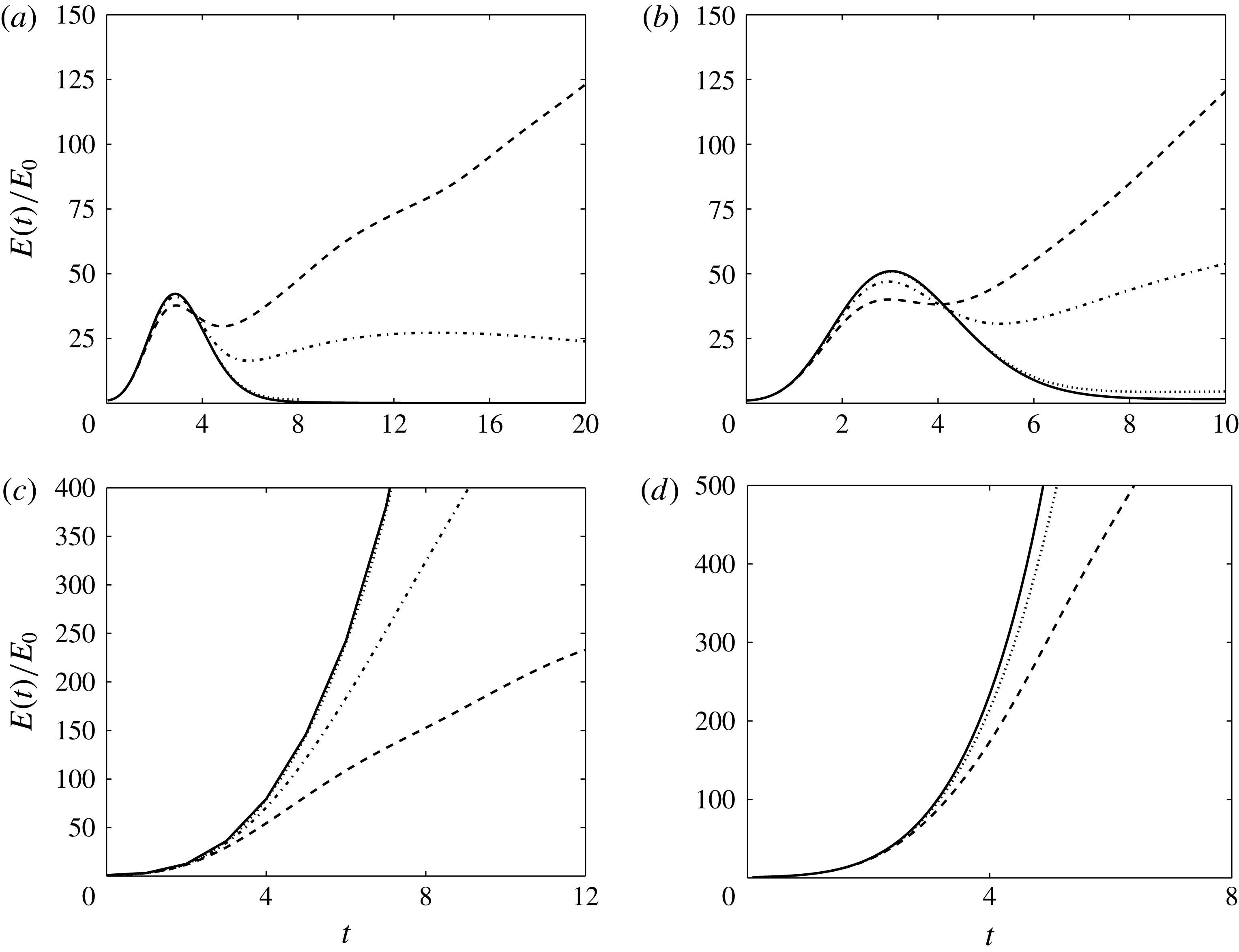
(see Alamo & Jimenez (Reference Alamo and Jimenez2003) for instance). The latter remark may give us some confidence that the spanwise extension considered in our case is sufficient. The time evolution of the kinetic energy associated with flow disturbances are extracted from DNS by subtracting the instantaneous state of the velocity field from the secondary base flow. In figure 24(a,b), we report time evolutions of kinetic energy disturbances associated with
 $V_{11}$
and
 $V_{12}$
(i.e.
 $t_{opt}=2$
) for
 $A_{0}=0.015$
and
 $A_{0}=0.025$
, respectively. One may recall that for
 $A_{0}=0.015$
the secondary base flow is asymptotically stable with respect to varicose perturbations in a local framework, and for
 $A_{0}=0.025$
two types of optimal wavepackets (i.e.
 $V_{12}$
and
 $V_{22}$
) coexist. We first focus on the flow case
 $A_{0}=0.015$
depicted in figure 24(a). For
 $E_{0}$
below
 $2.5\times 10^{-7}$
, the kinetic energy for disturbances is damped for long times. When the initial amplitude of the mode is increased above the former value, we observe a strong increase in kinetic energy around
 $t=5$
where the curve departs from the linear regime. Figure 24(b) shows results for the flow case
 $A_{0}=0.025$
. For the smallest amplitude
 $E_{0}=10^{-8}$
, the kinetic energy evolution exhibits a similar behaviour to the one obtained in a linear framework. When the initial amplitude of the optimal mode is fixed to
 $E_{0}=2.5\times 10^{-7}$
, the kinetic energy undergoes a different path. For
 $t>5$
, while disturbances are temporally damped in the linear regime, a growth of the kinetic energy is observed due to nonlinearities. As can be expected, the critical initial energy for disturbances to trigger a subcritical secondary instability is increased when the streak amplitude decreases. Furthermore, for
 $V_{11}$
and
 $V_{12}$
, nonlinear trajectories are seen to be separated by an edge state for given values of
 $A_{0}$
and
 $E_{0}$
(see Duguet et al. (Reference Duguet, Schlatter, Henningson and Eckhardt2012) for instance).
Nonlinear simulations. Integrated kinetic energy for the perturbation versus time: (a)
 $V_{11}$
; (b)
 $V_{12}$
; (c)
 $V_{22}$
and (d)
 $S$
. Curves are for
 $E_{0}=10^{-8}$
(dotted),
 $E_{0}=2.5\times 10^{-7}$
(dot-dashed) and
 $E_{0}=10^{-6}$
(dashed). The full line represents the linear evolution.

Varicose case
 $V_{12}$
. Nonlinear simulation for
 $E_{0}=10^{-6}$
. Visualization is restricted to one low-speed streak. The coherent structures are identified with isosurfaces of
 $\unicode[STIX]{x1D706}_{2}$
criterion in (a) and (b) for
 $t=3.5$
and
 $t=5.75$
, respectively, coloured by the distance from the lower wall. The vector field
 $(w,v)$
in the cross-section
 $(z,y)$
is shown for
 $t=3.5$
and
 $t=5.75$
at
 $x_{i}=4$
and
 $x_{i}=5.8$
in (c) and (d), respectively, where
 $w=\overline{W}-W$
and
 $v=\overline{V}-V$
.

Hereafter, we restrict our analysis to
 $A_{0}=0.025$
. We plot in figure 24(c,d), the time evolution of kinetic energy associated with disturbances for modes
 $V_{22}$
and
 $S$
. For both modes, nonlinearities have a stabilizing effect characteristic of a supercritical behaviour.
Figure 25(a,b) shows vortical structures at
 $t=3.5$
and
 $t=5.75$
associated with the nonlinear development of
 $V_{12}$
for
 $E_{0}=10^{-6}$
. For short times, the effect of Orr/lift-up mechanisms on the low-speed streak produces a slightly inclined streamwise vortex pair (see figure 25
a). As time evolves, between the two legs of the vortex pair, fluid is pumped up and backwards. It induces the formation of a hairpin head that is lifted up from the wall and shaped into a ring vortex as shown in figures 25 and 26. This event (
 $u<0$
,
 $v>0$
;
 $Q_{2}$
event in the quadrant analysis) is accompanied by an abrupt increase in the kinetic energy associated with disturbances as reported in figure 24(b). Further downstream (see figure 27), we observe that the vortex legs collide due to self-induction and generate a secondary hairpin vortex. This mechanism has already been observed in a fully turbulent regime by Zhou et al. (Reference Zhou, Adrian, Balachandar and Kendall1999). This whole process takes place in a region where linear analysis of secondary base flow concludes that there is asymptotic stability in a local framework. This hairpin regeneration is still accompanied with an increase in kinetic energy for disturbances.
Varicose case
 $V_{12}$
. Nonlinear simulation for
 $E_{0}=10^{-6}$
. Vector plots of perturbation velocity (
 $u=\overline{U}-U$
and
 $v=\overline{V}-V$
) on an
 $(x,y)$
plane extracted at the centre of a low-speed streak.

Varicose case
 $V_{12}$
. Nonlinear simulation for
 $E_{0}=10^{-6}$
. Visualization is restricted to one low-speed streak. The coherent structures are identified with isosurfaces of
 $\unicode[STIX]{x1D706}_{2}$
criterion in (a), (b), (c) and (d) for
 $t=7.5$
, 8, 8.5 and 9, respectively, coloured by the distance from the lower wall.

Regarding
 $V_{22}$
, a different behaviour is observed. For short times, the varicose wavepacket
 $V_{22}$
grows rapidly under the action of a quasi-exponential instability. When nonlinearities play a significant role, the mode exhibits a train of arch-like structures as shown in figure 28(a). By contrast with
 $V_{12}$
, vortical structures for
 $V_{22}$
are not attached to the wall and arches are not self-generated from one flow pattern but rather result from nonlinear saturation effects of the instability mode. Figure 28 also shows that characteristic structures of
 $V_{22}$
are quasi-streamwise vortices joining in the middle of the low-speed streak and also vortices pointing downstream taking a V shape. These vortices are very similar to those observed in the simulations of varicose streak breakdown for a flat-plate boundary layer by Brandt (Reference Brandt2007). Owing to nonlinearities, both
 $V_{22}$
and
 $V_{12}$
exhibit a bridge-like structure connecting quasi-streamwise vortices identified on both sides of the low-speed streak in the linear regime.
Nonlinear simulation for
 $E_{0}=10^{-6}$
: (a) varicose mode
 $V_{22}$
; (b) sinuous mode
 $S$
. Visualization is restricted to one low-speed streak. The coherent structures are identified with isosurfaces of
 $\unicode[STIX]{x1D706}_{2}$
criterion for
 $t=5$
coloured by the distance from the lower wall.

The initial stage of the nonlinear evolution of
 $S$
is shown in figure 28(b). The underlying vortical structures take the form of quasi-streamwise vortices located on both sides of the low-speed streak. In particular, vortices alternating in the streamwise direction are localized the centre of the low-speed streak. The latter nonlinear sinuous scenario exhibits close similarities with the sinuous streak breakdown described by Brandt & Schlatter (Reference Brandt and Schlatter2004) for the case of a flat-plate boundary layer.
5 Paths to turbulence
In the previous section, the different optimal wavepackets have been described during the first stages of the nonlinear regime. We now have to follow them further in time so as to know whether they evolve to turbulence. Hereafter, only the case
 $A_{0}=0.025$
is considered. Let us first examine the evolution of instantaneous flow structures as the wavepacket evolves along the streamwise direction. We show in figures 29–31 instantaneous snapshots of vortical structures developing inside the boundary layers for
 $V_{12}$
,
 $V_{22}$
and
 $S$
at times
 $t=20$
, 40 and 60. In figures 29–31, the flow structures are visualized by the
 $\unicode[STIX]{x1D706}_{2}$
criterion coloured by the distance from the lower wall. Figure 29 shows that, for
 $t=20$
and
 $V_{12}$
, the subcritical mechanism described in the previous section has led to the formation of a hairpin train similar as the mechanism described by Zhou et al. (Reference Zhou, Adrian, Balachandar and Kendall1999).
For
 $E_{0}=10^{-6}$
, isosurfaces of the
 $\unicode[STIX]{x1D706}_{2}$
criterion are shown coloured by the distance from the lower wall at
 $t=20$
for
 $V_{12}$
,
 $V_{22}$
and
 $S$
(a–c).

For
 $E_{0}=10^{-6}$
, isosurfaces of the
 $\unicode[STIX]{x1D706}_{2}$
criterion are shown coloured by the distance from the lower wall at
 $t=40$
for
 $V_{12}$
,
 $V_{22}$
and
 $S$
(a–c).

For time
 $t=40$
(figure 30), the wavepacket spreads streamwise, and we observe a turbulent puff in the centre of the latter surrounded by more quiet phases upstream and downstream. Furthermore, while the leading edge of the wavepacket is dominated by ring-like structure (or
 $\unicode[STIX]{x1D6FA}$
vortices) extending near the wall, the downstream part is characterized by arch-like structures (i.e. not attached to the wall) developing in the outer part of the boundary layer. For time
 $t=60$
(figure 31), we observe that the puff has spread in the streamwise direction and that arch-like structures predominate. This laminar–turbulent transition process is similar to the one described by Eitel-Amor, Flores & Schlatter (Reference Eitel-Amor, Flores and Schlatter2014), where the authors investigate the flat-plate boundary layer case. When considering transition induced by
 $V_{22}$
, figures 29–31 show that for
 $t=20$
the flow is populated by trains of arch-like structures. Their tips are deformed into vortex-ring types and tilted upward from the wall in the outer part of the boundary layer. In the centre of the wavepacket, ring-like structures split generating harmonics, a fact that is not observed for
 $V_{12}$
at the same time. At
 $t=40$
, arch-like structures predominate in the flow and we observe the breakdown of the spanwise symmetry. For
 $t=60$
, the wavepacket extends over a larger distance than the one associated with
 $V_{12}$
.
For
 $E_{0}=10^{-6}$
, isosurfaces of the
 $\unicode[STIX]{x1D706}_{2}$
criterion are shown coloured by the distance from the lower wall at
 $t=60$
for
 $V_{12}$
,
 $V_{22}$
and
 $S$
(a–c).

For the nonlinear evolution of the sinuous mode
 $S$
, figures 29–31 show that for
 $t=20$
higher harmonics are generated than for the case
 $V_{22}$
at the same time. In addition, flow already breaks symmetry in the spanwise direction at this time. We also observe that, while the leading edge of the wavepacket is characterized by a sinuous motion, the centre of the latter is dominated by similar coherent motions as the one observed for
 $V_{12}$
and
 $V_{22}$
, such as arch-like structures. This gives some arguments that, for both scenarios,
 $V_{12}$
,
 $V_{22}$
and
 $S$
evolve into a unique turbulent state as also observed by Eitel-Amor et al. (Reference Eitel-Amor, Flores and Schlatter2014) and Sayadi, Hamman & Moin (Reference Sayadi, Hamman and Moin2013) in the case of a turbulent flat-plate boundary layer.
In figure 32, we show the skin friction
 $C_{f}$
as a function of
 $x_{i}$
for the different modes. For comparison purposes, we also report
 $C_{f}$
values found in the literature for the laminar case and for a turbulent boundary layer without pressure gradient (see Schlatter & Orlu (Reference Schlatter and Orlu2010) for instance). The spanwise average instantaneous streamwise velocity is considered to evaluate the skin friction coefficient. Considering that
 $C_{f}$
provides an indication of the transition location, figure 32 shows that, for
 $t=48$
, transition occurs for both
 $S$
and
 $V_{22}$
. For
 $V_{12}$
, transition is established for
 $t>50$
. The latter remark is consistent with the discussion above related to the observation of coherent structures. It is also interesting to note that the subcritical transition provided by
 $V_{12}$
yields similar
 $C_{f}$
as for
 $S$
and
 $V_{22}$
cases. For both cases, while, for the lower wall, transition is observed for
 $t=64$
and later, the transition is not yet triggered for the boundary layer developing along the upper wall.
For
 $E_{0}=10^{-6}$
, the skin friction coefficient versus the streamwise position for
 $t=48$
, 64 and 72 (dotted, full and dashed lines, respectively). Distributions of
 $C_{f}$
for the laminar and turbulent cases are also reported. (a)
 $V_{12}$
, (b)
 $V_{22}$
and (c)
 $S$
.

For each turbulent wavepacket, statistics are accumulated for the same given streamwise position
 $x_{i}=66$
by averaging along the spanwise direction and on a specific time interval. The time window is set on a criterion based on the value of
 $C_{f}$
that corresponds to the turbulent case. Samples are based on 100 time values and 96 sections in the spanwise direction. The friction Reynolds number (i.e. based on the friction velocity, the half-channel height and the kinematic viscosity) at the lower wall is found for all flow cases equal to
 $Re_{\unicode[STIX]{x1D70F}}=166$
. Hereafter, the superscript
 $+$
will denote quantities scaled in inner units. Figure 33 shows the mean streamwise velocity profile in the wall-normal direction. For the lower wall, it exhibits a flatter profile in comparison with its upper wall counterpart. It gives some evidence that the flow evolves to a turbulent regime on the lower wall. To further investigate the latter remark, we report in figure 34, the streamwise average velocity together with the root-mean-square (r.m.s.) velocities as a function of the distance from the lower wall in inner units. For comparison purposes, results provided by Moser, Kim & Mansour (Reference Moser, Kim and Mansour1998) and Schlatter & Orlu (Reference Schlatter and Orlu2010) for a turbulent channel flow at
 $Re_{\unicode[STIX]{x1D70F}}=180$
and a turbulent flat-plate boundary layer at
 $Re_{\unicode[STIX]{x1D70F}}=252$
are also shown. Despite the lack of convergence of statistics due to the small data samples that are collected, a good agreement for the mean velocity profile is observed in figure 34(a,c,e). Regarding the variance of the mean velocity components, figure 34(b,d,f) shows that profiles are also in good agreement with the literature. In particular, the streamwise velocity dominates in the r.m.s. values and it peaks at a distance from the lower wall in inner units
 $y^{+}\approx 13$
. It indicates that streaks associated with a self-sustained process in the buffer region are present, which is a universal characteristic of wall turbulence (Hamilton, Kim & Waleffe Reference Hamilton, Kim and Waleffe1995). Hence, it shows that statistics converge to the same turbulent values in each case considered. Finally, for all flow cases, we note that turbulent coherent structures populating the outer part of the boundary layer have not yet triggered turbulent transition of the boundary layer developing on the upper wall. It gives some insight into the fact that the turbulent transition of boundary layers developing along the upper and lower walls in the entrance channel flow can remain uncoupled over a long distance.
For
 $E_{0}=10^{-6}$
and
 $x_{i}=66$
, the mean streamwise velocity made dimensionless by
 $u_{\unicode[STIX]{x1D70F}}$
estimated at
 $y=-1$
. The full line shows the distributions of
 $U^{+}$
for a fully developed turbulent channel flow at
 $Re_{\unicode[STIX]{x1D70F}}=180$
and for the laminar entrance channel flow. (a)
 $V_{12}$
, (b)
 $V_{22}$
and (c)
 $S$
.

Results for
 $E_{0}=10^{-6}$
and
 $x_{i}=66$
. Dashed lines: (a,c,e) mean streamwise velocity profiles versus distance from the wall in inner units; (b,d,f) r.m.s. profiles versus distance from the wall in inner units. Profiles for a fully developed turbulent channel flow at
 $Re_{\unicode[STIX]{x1D70F}}=180$
and a turbulent flat-plate boundary layer at
 $Re_{\unicode[STIX]{x1D70F}}=252$
are also reported in full and dotted lines, respectively. (a,b)
 $V_{12}$
, (c,d)
 $V_{22}$
and (e,f)
 $S$
.

6 Conclusions
This work aims at describing different paths leading to turbulence for the entrance channel flow case associated with uniform upstream flow conditions. Bypass transition is investigated in the light of secondary perturbation analysis for low-speed streaks. They are spatially amplified downstream with a close resemblance to developing streaks behind a roughness element. The resulting turbulent transition occurs in the developing boundary layers, before the formation of the Poiseuille regime. In this context, specific attention has been paid to understand both linear and nonlinear mechanisms bringing the system to transition.
Linear global optimizations on the streaky base flow are performed, consisting in searching for initial perturbations having the largest energy growth for given times. Specifically, we consider varicose and sinuous symmetry separately and only the fundamental case (i.e. streaks and perturbations have the same spanwise periodicity). Optimal perturbations at the initial time take the form of localized wavepackets for all cases. Sinuous wavepackets are dominant for the lowest streak amplitude whereas the varicose secondary perturbation is the most amplified for the largest streak amplitude. However, for short optimization times, varicose and sinuous optimal wavepackets attain comparable gain in energy. Interestingly, while the sinuous optimal wavepacket is not too affected by time optimization, varicose ones exhibit two different behaviours. For short optimization times, the varicose perturbation at initial time is localized in the flanks of the low-speed streak near the inlet, and for larger target times, the initial wavepacket is concentrated downstream, where streaks are subject to exponential instability. For the sinuous wavepacket, the linear mechanism responsible for energy growth is mainly associated with spanwise shear and especially the presence of inflection points along the spanwise direction, as usually found for streak instability. For the varicose symmetry, in the linear regime, the optimal perturbation corresponding to short target times extracts energy from the base flow by combining Orr and lift-up mechanisms. By inspecting the vorticity budget, it is shown that the lift-up mechanism is governed by a vortex-tilting term associated with the spanwise shear. For larger optimization times, the energy growth is associated with the presence of an inflection point in the wall-normal direction as revealed by the kinetic energy production terms distribution in the cross-sections.
By means of DNS, the nonlinear space–time dynamics of optimal wavepackets is investigated. We observe the existence of a path to turbulence that is subcritical with respect to secondary modal instability for the varicose wavepacket associated with short optimization time. This path includes nonlinear interactions of pairs of oblique waves located on the flanks of the low-speed streak. Similarly as the oblique wave transition case (see Schmid & Henningson Reference Schmid and Henningson1992), a strong increase of the perturbation kinetic energy that escapes from the laminar attractor is observed. This nonlinear path leads to hairpin trains that break down to turbulence downstream. For larger optimization times, perturbations are dominated by modal instability and nonlinearities first have a damping effect on the energy growth of perturbation, typical of supercritical behaviour. As the perturbation moves downstream, the varicose optimal wavepacket leads to arch-like structures in the outer part of the boundary layer, and spanwise oscillating streaks are observed for the sinuous one. Further downstream, we observe the convergence to typical wall-bounded turbulent flow profiles (mean flow and r.m.s.) for all cases. In this stage, the outer part of the boundary layer is dominated by arch-like patterns independently of the symmetry of the initial wavepacket.
These results lead us to some conclusions: (i) The entrance channel flow may exhibit laminar–turbulent transition well before the merging of the developing boundary layers. (ii) The fully developed turbulent region exhibits similar statistics as those associated with more classic wall-bounded turbulent flows. As a consequence it seems difficult to distinguish whether or not the turbulent transition observed in channel flow experiments is due to entrance effects. (iii) Varicose wavepackets associated with short optimization times are localized near the inlet and have comparable gains with their sinuous counterparts. It further indicates that under certain conditions of external perturbations, the varicose scenario leading to streak breakdown and turbulence can be viable even if streaks are stable with respect to modal instability under the parallel flow assumption. (iv) For the values of
 $Re$
and
 $x_{0}$
(i.e. streamwise abscissa of the initial vortex pair generating streaks) that are considered, the upper and lower boundary layers are weakly mutually dependent. The present study brings some light on the transient varicose instability observed by Buffat et al. (Reference Buffat, Le Penven, Cadiou and Montagnier2014) using DNS. In this respect, the use of global optimization gives an accurate description of the transient/convective instability mechanism in a region where non-parallelism effects cannot be neglected. Nevertheless, questions remain unanswered. Among them, one may ask if there is an optimal set of amplitudes for primary and secondary disturbances to trigger laminar–turbulent transition. It could thus be an interesting prospect to investigate what is the initial finite-amplitude perturbation including both streamwise vortices and secondary perturbations that is the most dangerous (i.e. with the smallest initial energy level to lead to turbulence). In particular, how affected is the subcritical varicose scenario leading to hairpin vortices for such an optimal range of parameters? Can we provide some criteria for choosing amplitude parameters that trigger transition the most rapidly? Since boundary-layer-like flows are receptive to low- and high-frequency modes, their natural excitation may contain a subset of primary and secondary perturbations. Identifying an optimal set of streak and secondary perturbation amplitudes could thus be a promising route to better characterize whether or not transition is expected to occur before the fully developed region when the flow is exposed to free-stream turbulence.
It is worth noting that the transient growth varicose path cannot trigger transition in the absence of nonlinearities. In this context, Cherubini et al. (Reference Cherubini, Palma, Robinet and Bottaro2010) show that, in a flat boundary layer, finite-amplitude perturbation obtained from nonlinear global optimization is capable of inducing laminar–turbulent transition for initial energy much lower than its linear counterpart (see also Pringle & Kerswell (Reference Pringle and Kerswell2010) for the pipe flow case). The authors found that the optimal perturbation is strongly localized in both streamwise and spanwise directions and it takes the form of a low-momentum region flanked by two series of inclined streamwise-alternated elongated patches. In addition, Cherubini et al. (Reference Cherubini, Palma, Robinet and Bottaro2010) show that the different components of the perturbation have comparable amplitudes at the initial time. Far downstream, hairpin vortices that break down to turbulence are found. While the nonlinear optimal trajectory strongly differs from the scenario based on streak bifurcation due to a secondary exponential growth, it shares some similarities with the subcritical varicose path shown in the present analysis. In particular, they exhibit both localized inclined patches of streamwise-alternated perturbations flanked on both sides of a low-momentum region, and breakdown to turbulence induced by hairpin vortices. One may thus ask whether or not nonlinear optimizations in the entrance channel flow will lead to a similar initial perturbation to the one provided by an optimal set of initial amplitudes for primary and secondary perturbations of streaks.
The present work focuses only on a specific choice of inflow condition and aspect ratio (
 $\unicode[STIX]{x1D6FF}^{\star }/h$
). Parametric investigation remains to be done, in particular to explore how the mutual interaction between the upper and lower boundary layers and the induced favourable pressure gradient affect the instabilities for different choices of aspect ratio. In the turbulent regime, Dixit & Ramesh (Reference Dixit and Ramesh2010) have recently shown, from experimental data, that accelerating turbulent boundary layers exhibit changes in coherent motions populating the outer region while the inner region is not modified. In agreement with these observations, the near-wall region in the present study exhibits the same statistics as the ones of a flat-plate boundary layer without pressure gradient, but it gives no further indication about the outer layer dynamics due to the low Reynolds number considered here. Hence, different behaviour could be expected for higher Reynolds number flows.
Finally, Sadri & Floryan (Reference Sadri and Floryan2002) show that, for upstream conditions associated with a sharp-edge channel, the flow exhibits separation zones on both walls that extend far downstream when increasing the Reynolds number. Hence, a different scenario leading to turbulence for such entrance channel flow solution may be suggested, strongly connected to separated flow unsteadiness similar as those reported by Passaggia, Leweke & Ehrenstein (Reference Passaggia, Leweke and Ehrenstein2012).
Acknowledgements
This work was performed using HPC resources from the FLMSN.