



1. Introduction
Flows in natural and engineered channels are often partially obstructed by arrays of elements, such as vegetation patches, roughness clusters or porous obstacles. The drag contrast between the obstructed and unobstructed regions generates a lateral shear layer that regulates momentum exchange, turbulence production and scalar transport (Nepf Reference Nepf2012). The interaction between flows and obstacles spans a wide range of configurations and is relevant to different flow regimes, including jet-like flows (Mossa et al. Reference Mossa, Goldshmid, Liberzon, Eletta Negretti, Sommeria, Termini and De Serio2021) and wave-driven dynamics (Mossa et al. Reference Mossa, De Padova and Onorato2025). As sketched in figure 1, a canonical two-layer organisation emerges: an inner region within the obstacle array dominated by form drag and wake interactions, and an outer region in the free stream governed by depth-induced shear. The mean lateral velocity transition is typically inflectional and exhibits coherent vortices, enhanced mixing and intensified interfacial shear stresses relative to smooth-wall flows (Ghisalberti & Nepf Reference Ghisalberti and Nepf2002; White & Nepf Reference White and Nepf2007). These Kelvin–Helmholtz (KH)-like features highlight the need for a consistent theoretical and numerical framework to interpret interfacial dynamics.
Previous studies have established a consistent phenomenology of canopy and vegetated shear layers, including the classical mixing-layer analogy, the emergence of coherent interfacial structures and scaling relations for the growth of the shear-layer thickness (e.g. Ghisalberti & Nepf Reference Ghisalberti and Nepf2002; White & Nepf Reference White and Nepf2007; Nepf Reference Nepf2012). Several interpretations have been proposed to explain the origin of these structures, often drawing on analogies with free shear layers. Despite this substantial body of work, a key question remains unresolved: whether the observed KH-like vortices in shallow, partially obstructed flows arise from a classical inviscid KH instability or from a drag-modified instability mechanism specific to shallow-water environments.
At the continuum scale, homogenised closures such as Brinkman-type extensions of Darcy’s law describe the resistance of dense arrays and clarify how porous layers transmit and dissipate shear (Brinkman Reference Brinkman1949). In shallow configurations with sharp lateral drag contrast, the resulting two-layer shear mixing structure closely resembles that of canopy flows. The present framework therefore applies not only to vegetated channels, but also to generic arrays of emergent rigid obstacles.
An example involving vegetation is shown in figure 2, where a free stream interacts with a densely obstructed patch. Although the present work focuses on rigid cylinders, the same interfacial geometry arises across a broad family of systems, including aquatic or terrestrial vegetation, high-porosity engineered media and certain biological interfaces. The endothelial glycocalyx, for example, behaves as a porous resistive lining adjacent to a viscous free stream (Weinbaum et al. Reference Weinbaum, Tarbell and Damiano2007). Although the microvascular regime is laminar whereas the present shallow flows are turbulent, the geometric organisation of a free stream coupled to a resistive sublayer is analogous, and similar momentum-exchange mechanisms arise across the interface.
Schematic of two side-by-side streams. The
 $x$
-axis lies along the interface (
 $y=0$
); the shear layer develops only in the unobstructed region with a thickness
 $\delta (x)$
increasing downstream. Interface arrows depict lateral transfer from the obstructed to the unobstructed side, with decreasing slope along
 $x$
.

Figure 1. Long description
Schematic of two side-by-side streams. The $x$-axis lies along the interface ($y=0$); the shear layer develops only in the unobstructed region with a thickness δ$(x)$ increasing downstream. Interface arrows depict lateral transfer from the obstructed to the unobstructed side, with decreasing slope along $x$.
Vegetated vs. non-vegetated patch; interface at
 $y=0$
.

Figure 2. Long description
Vegetated vs. non-vegetated patch; interface at $y=0$.
This study addresses this issue by combining a two-layer theoretical framework, laboratory experiments and graphics processing unit (GPU)-accelerated smoothed particle hydrodynamics (SPH) simulations to provide a unified interpretation of the interfacial shear-layer dynamics. In particular, the work aims to: (i) characterise the mean velocity structure and associated momentum balance at the interface, (ii) quantify the role of the coherent sweep–ejection dynamics in momentum transfer and mixing and (iii) assess the instability mechanism governing the observed KH-like structures through both classical Rayleigh analysis and a drag-modified shallow-water formulation. This approach allows a clear distinction between established phenomenology and the specific contributions of the present study, including the analysis of measured profiles, the finite control-volume formulation of interfacial energetics and the interpretation of Lagrangian transport in relation to coherent structures.
Building on this perspective, the present work examines the interfacial shear layer in a shallow channel partially obstructed by a uniform array of emergent rigid cylinders. High-resolution GPU-accelerated SPH simulations are combined with a two-layer analytical framework and laboratory measurements in an unusually wide (4 m) flume. We address the following questions: (i) How accurately a hyperbolic–tangent profile represents the lateral velocity across the interface over a wide streamwise range; (ii) how the inferred shear-layer thickness and outer-edge velocity evolve downstream and govern interfacial shear stress and momentum exchange; (iii) how the sweep–ejection dynamics organises interfacial Reynolds stresses and whether a finite-amplitude equilibrium persists; and (iv) how lateral detrainment and pressure gradients enter a momentum integral balance tailored to shallow obstructed flows.
In this broader context, the study aims to generalise canopy-flow concepts to a wider class of obstacle-induced shallow flows and to clarify the dynamical organisation of the interfacial vortices that dominate momentum exchange. Although previous experimental and numerical studies have documented the emergence of coherent KH-like structures at obstructed free-stream interfaces (e.g. White & Nepf Reference White and Nepf2007), the physical origin of these motions has remained ambiguous. In particular, it has been unclear whether the observed interfacial rollers arise from a classical inviscid KH instability or from a distinct mechanism associated with obstacle-induced drag.
In this context, we examine whether the observed KH-like structures can be explained within a classical inviscid framework or require a drag-modified interpretation. Classical Rayleigh analysis is therefore applied to the measured profiles, and the results are interpreted within the framework of the shallow-water modified Rayleigh equation.
The paper is organised as follows. Section 2 introduces the theoretical framework; § 3 summarises the methodology; § 4 couples simulations, theory and measurements; § 5 investigates the sweep–ejection dynamics; § 6 examines coherent structures; and § 7 presents the Lagrangian dispersion analysis. Section 8 discusses the drag-modified stability mechanisms, and conclusions are given in § 9. For completeness, Appendix A provides a detailed derivation of the interfacial momentum balance, and Appendix B summarises the derivation of the classical Rayleigh equation and its shallow-water drag-modified counterpart.
2. Theoretical model
2.1. Formulation of the shear-layer model
Figure 3 shows a shallow flow partially obstructed by emergent rigid obstacles. The streamwise and transverse coordinates are denoted by
 $x$
and
 $y$
, with the origin located at the interface between the obstructed region (width
 $B_o$
) and the unobstructed one (width
 $B_u$
). As in previous studies, the mean velocity is lower inside the obstacle array and higher in the free-stream region, generating an interfacial shear layer of finite thickness.
Sketch of the flow with obstructed and unobstructed areas.

Figure 3. Long description
Sketch of the flow with obstructed and unobstructed areas.
To analyse momentum exchange across this interface, we consider an infinitesimal control volume of streamwise length
 $\text{d}x$
and unit depth located within the shear layer separating the obstructed and unobstructed parts of the channel (figure 4). Within this region, obstacle-induced drag produces a velocity deficit and a strong interfacial momentum transfer between the two zones.
Infinitesimal control volume of the shear layer for the analysis of acting forces.

Figure 4. Long description
Infinitesimal control volume of the shear layer for the analysis of acting forces.
Reference should be made to figures 4 and 5 for the coordinate system and symbols used. The velocities
 $u$
and
 $v$
denote the instantaneous velocity components in the streamwise (
 $x$
) and transverse (
 $y$
) directions, respectively, while
 $u'$
and
 $v'$
represent their turbulent fluctuations. In the following, the overbar symbol or the capital letters will be used to indicate time-averaged quantities. Under the assumptions of steady, two-dimensional, depth-averaged flow, the integral momentum balance applied to the control volume shown in figure 5 may be written as
 \begin{align} \text{d}\boldsymbol{F} + \text{d}\boldsymbol{F}_\tau + \text{d}\boldsymbol{F}_\varepsilon + \text{d}\boldsymbol{M}_{\textit{in}} + \text{d}\boldsymbol{M}_{\textit{out}} = \boldsymbol{0}, \end{align}
where
 $\text{d}\boldsymbol{F}$
and
 $\text{d}\boldsymbol{F}_\tau$
denote the pressure and shear forces acting on the control surfaces,
 $\text{d}\boldsymbol{F}_\varepsilon$
is a force-equivalent term accounting for the mechanical losses induced by the stems and their wakes and
 $\text{d}\boldsymbol{M}_{\textit{in}}$
and
 $\text{d}\boldsymbol{M}_{\textit{out}}$
are the momentum fluxes entering and leaving the control volume.
Forces acting on the infinitesimal control volume of the boundary layer.

Figure 5. Long description
Forces acting on the infinitesimal control volume of the boundary layer.
The detailed geometric evaluation of the pressure and mass-flux contributions across the inclined control surface is reported in Appendix A. Retaining only first-order terms in
 $\text{d}x$
, the streamwise momentum balance becomes
 \begin{align} \frac {\textrm{d}{F}_\varepsilon }{\text{d}x} -\frac {\text{d}\overline {p}}{\text{d}x} \delta - \overline {\tau }_0 = \frac{\text{d}}{\text{d}x} \left ( \int _{0}^{\delta (x)} \rho \overline {u}^2 \, \text{d}y \right ) - \overline {u}_{\kern-1pt f} \frac{\text{d}}{\text{d}x} \left ( \int _{0}^{\delta (x)} \rho \overline {u} \, \text{d}y \right ) + \rho \overline {u}_{y0} \overline {v}_{y0}, \end{align}
where
 $\delta (x)$
is the local shear-layer thickness,
 $\rho$
is the water density,
 $\overline {u}_{\kern-1pt f}$
is the velocity at the outer edge of the control volume and
 $\overline {u}_{y0}$
,
 $\overline {v}_{y0}$
denote the velocity components at the interface
 $y=0$
.
Rearranging terms gives the interfacial shear stress
 \begin{align} -\overline {\tau }_0(x) = -\frac {\textrm{d}{F}_\varepsilon }{\text{d}x} + \frac {\text{d}\overline {p}}{\text{d}x}\,\delta (x) + \frac{\text{d}}{\text{d}x} \left [ \int _{0}^{\delta } \rho \big ( \overline {u}^2 - \overline {u}_{\kern-1pt f} \overline {u} \big ) \, \text{d}y \right ] + \rho \overline {v}_{y0}^2. \end{align}
For a discrete interfacial cell whose streamwise size coincides with the spacing between two consecutive stems, denoted by
 $s$
(figure 6), the balance may be written as
 \begin{align} \frac {\Delta {F}_\varepsilon }{\Delta x} = \overline {\tau }_0(x) + \frac {\Delta \overline {p}}{\Delta x} \delta (x) + \frac {\varDelta }{\Delta x} \left [ \int _{0}^{\delta } \rho \big ( \overline {u}^2 - \overline {u}_{\kern-1pt f} \overline {u} \big ) \, \text{d}y \right ] + \rho \overline {v}_{y0}^2. \end{align}
Cell element at the boundary that includes a stem with its wake.

Figure 6. Long description
Cell element at the boundary that includes a stem with its wake.
To estimate the dissipation
 $\varepsilon _{\textit{FCV}}$
associated with the finite control volume, we consider that the dissipated power per unit depth over an area
 $W=\Delta x\,\delta (x)$
is of order
 \begin{align} P = \mathcal{O}\left (\rho \,\varepsilon _{\textit{FCV}}\, W\right ), \end{align}
while the same power may also be expressed as the product of the dissipative force and a characteristic interfacial velocity scale
 $\mathcal{U}$
, namely
 \begin{align} P=\mathcal{O}\left (\Delta {F}_\varepsilon \, \mathcal{U}\right ). \end{align}
Hence,
 \begin{align} \varepsilon _{\textit{FCV}}= \mathcal{O}\left (\frac {\Delta {F}_\varepsilon \, \mathcal{U}}{\rho \,W}\right )\!. \end{align}
The quantity
 $\varepsilon _{\textit{FCV}}$
should therefore be interpreted as a control-volume estimate of the mechanical energy removed from the mean flow by stem–wake interaction, pressure-gradient work and lateral detrainment. It is not a pointwise viscous dissipation, but rather a mechanically based energetic diagnostic at the scale of the interfacial cell.
2.2. Hyperbolic–tangent velocity profile
Following White & Nepf (Reference White and Nepf2007), the mean velocity across the obstructed/unobstructed interface is expressed as a laterally averaged profile, i.e. averaged in the transverse direction across the obstacle array. This representation does not resolve the local oscillatory structure of the velocity field within the obstructed region, where the presence of discrete stems induces a sub-stem-scale modulation with near-zero velocities at the stem locations and local maxima in the gaps between consecutive stems. Nevertheless, this averaged description provides physically meaningful information for the present analysis, where the primary interest lies in the overall flow behaviour rather than in the detailed flow field at the scale of individual stems. Accordingly, following White & Nepf (Reference White and Nepf2007), the mean velocity across the obstructed/unobstructed interface is expressed as
 \begin{align} U(y) = U_m + A\,\tanh \!\left (\frac {y}{b}\right ), \qquad U_m = \frac {U_o + U_{\textit{obs}}}{2}, \qquad A = \frac {U_o - U_{\textit{obs}}}{2}, \end{align}
where
 $U_o$
and
 $U_{\textit{obs}}$
are the characteristic velocities of the unobstructed and obstructed regions, respectively, and
 $b$
is the half-thickness of the shear layer. The local shear is
 \begin{align} \frac {\text{d}U}{\text{d}y} = \frac {A}{b}\,\mathrm{sech}^2\!\left (\frac {y}{b}\right )\!, \end{align}
with its maximum at
 $y=0$
, so that the corresponding vorticity thickness is
 \begin{align} \delta _\omega = \frac {U_o - U_{\textit{obs}}}{\max (\text{d}U/\text{d}y)} = 2b. \end{align}
In the integral formulation,
 $\delta (x)$
denotes an apparent mixing-layer thickness, here defined as the distance from the interface where the mean velocity reaches a prescribed fraction of
 $U_o$
. For the hyperbolic–tangent profile
 \begin{align} \frac {U(\delta _r) - U_m}{A} = \tanh \!\left (\frac {\delta _r}{b}\right ) = r \quad \Rightarrow \quad \delta _r = b\,\mathrm{atanh}(r). \end{align}
Using
 $r=0.99$
, one obtains
 \begin{align} \delta (x) = \delta _{0.99}(x) = 2.65\,b(x), \end{align}
and the outer-edge velocity is
 \begin{align} \overline {u}_{\kern-1pt f}(x) = U (\delta (x)) = U_m + A\,\tanh \!\left (\frac {\delta (x)}{b}\right )\!. \end{align}
2.3. Closed–form integrals and interfacial stress
Using the hyperbolic–tangent profile
 \begin{align} U(y,x)=U_m(x)+A(x)\tanh \!\left (\frac {y}{b(x)}\right )\!, \end{align}
the integrals in (2.2) and (2.3) can be written as
 \begin{align} \mathcal{I}_1(\delta )=\int _0^{\delta } U\,\text{d}y = U_m\,\delta + A\,b\,\ln \cosh \!\left (\frac {\delta }{b}\right )\!, \\[-28pt] \nonumber \end{align}
 \begin{align} \mathcal{I}_2(\delta )= \int _0^{\delta } U^2\,\text{d}y = U_m^2\,\delta + 2A\,U_m\,b\,\ln \cosh \!\left (\frac {\delta }{b}\right ) + A^2\!\left [\delta - b\,\tanh \!\left (\frac {\delta }{b}\right )\right ]\!. \\[0pt] \nonumber \end{align}
Defining
 $\mathcal{J}(\delta ;\overline {u}_{\kern-1pt f}) = \rho \,[\mathcal{I}_2(\delta ) - \overline {u}_{\kern-1pt f}\,\mathcal{I}_1(\delta )]$
, differentiation with respect to
 $x$
yields
 \begin{align} \frac {\text{d}\mathcal{J}}{\text{d}x} = -\,\rho \,\mathcal{I}_1(\delta )\,\frac {\text{d}\overline {u}_{\kern-1pt f}}{\text{d}x}, \end{align}
where the direct streamwise variations of
 $A(x)$
and
 $b(x)$
are assumed to be of higher-order terms in the local balance. The derivative of the outer-edge velocity is given by
 \begin{align} \frac {\text{d}\overline {u}_{\kern-1pt f}}{\text{d}x} = \left (\frac {\partial U}{\partial y}\right )_{y=\delta }\frac {\text{d}\delta }{\text{d}x} + \left (\frac {\partial U}{\partial x}\right )_{y=\delta }. \end{align}
Since the interfacial shear stress acts at
 $y=0$
, (2.9) gives
 \begin{align} \left (\frac {\text{d}U}{\text{d}y}\right )_{y=0} = \frac {A(x)}{b(x)}. \end{align}
Accordingly, (2.2) becomes
 \begin{align} \tau _0(x) = \frac {\text{d}F_\varepsilon }{\text{d}x} - \frac {\text{d}\overline {p}}{\text{d}x}\,\delta (x) + \rho \,\mathcal{I}_1 (\delta (x))\, \left (\frac {\text{d}U}{\text{d}y}\right )_{y=0} - \rho \,\overline {u}_{y0}(x)\,\overline {v}_{y0}(x), \end{align}
or equivalently
 \begin{align} \tau _0(x) = \frac {\text{d}F_\varepsilon }{\text{d}x} - \frac {\text{d}\overline {p}}{\text{d}x}\,\delta (x) + \rho \,\mathcal{I}_1 (\delta (x))\,\frac {A(x)}{b(x)} - \rho \,\overline {u}_{y0}(x)\,\overline {v}_{y0}(x). \end{align}
Combining (2.2), (2.15) and (2.21), the discrete cell balance leads to the estimate
 \begin{align} \varepsilon _{\textit{FCV}}\left (x\right ) \simeq \frac {U(x)}{\rho \,\delta (x)} \left [ \tau _0(x) + \frac {\Delta \overline {p}}{\Delta x}\,\delta (x) + \rho \,\overline {v}_{y0}^2(x) - \rho \,\mathcal{I}_1\!\big (\delta (x)\big )\,\frac {A(x)}{b(x)} \right ]\!. \end{align}
Equation (2.22) preserves the classical energetic structure of production, transport and loss terms, but it does so from the viewpoint of a finite interfacial control volume. This is the basis for the subsequent comparison with the dissipation reconstructed from the turbulent kinetic-energy budget.
2.4. Turbulent kinetic-energy balance
For reference, the turbulent kinetic-energy (TKE) balance is briefly recalled. For an incompressible flow, the TKE per unit mass is defined as
 \begin{align} k = \frac {1}{2}\,\overline {u_i' u_i'}. \end{align}
Its transport equation reads
 \begin{align} \frac {\partial k}{\partial t} + U_j\frac {\partial k}{\partial x_j} = -\,\overline {u_i' u_j'}\,\frac {\partial U_i}{\partial x_j} - \frac {\partial }{\partial x_j} \left ( \frac {\overline {u_j' p'}}{\rho } + \frac {1}{2}\overline {u_i' u_i' u_j'} \right ) - \varepsilon _{\textit{TKE}}, \end{align}
where the terms on the right-hand side represent, respectively, shear production, turbulent and pressure transport and viscous destruction of TKE.
Under the assumptions of a steady, two-dimensional flow in the
 $(x,y)$
plane, (2.24) reduces to the balance
 \begin{align} 0 = T_{\textit{ad}v} + T_{\textit{prod}} + T_{\textit{transp}} - \varepsilon _{\textit{TKE}}, \end{align}
where the individual contributions are
 \begin{align} T_{\textit{ad}v} = -U\,\frac {\partial k}{\partial x}, \qquad T_{\textit{prod}} = -\,\overline {u'v'}\,\frac {\partial U}{\partial y}, \qquad T_{\textit{transp}} = -\,\frac {\partial }{\partial y} \overline {v'\!\left (k+\frac {p'}{\rho }\right )}. \end{align}
Accordingly,
 \begin{align} \varepsilon _{\textit{TKE}} = T_{\textit{ad}v} + T_{\textit{prod}} + T_{\textit{transp}} . \end{align}
The two dissipation estimates introduced above quantify different physical mechanisms. The quantity
 $\varepsilon _{\textit{TKE}}$
is a local budget residual associated with the irreversible destruction of TKE, whereas
 $\varepsilon _{\textit{FCV}}$
is a control-volume estimate of the mechanical energy removed from the mean flow over an interfacial cell. Pointwise agreement between the two is therefore neither expected nor required. Since
 $\varepsilon _{\textit{FCV}}$
and
 $\varepsilon _{\textit{TKE}}$
originate from different governing equations and quantify different stages of the energy-transfer process, the purpose of their comparison is not to establish equality between the two quantities. Rather, it is to examine the physical consistency between the regions where the mean flow loses mechanical energy and those where TKE is subsequently produced and dissipated. In this sense, the finite control-volume (FCV) formulation is not intended to reproduce the fine-scale structure of
 $\varepsilon _{\textit{TKE}}$
, but rather to provide a mechanically grounded energetic diagnostic that can be evaluated from resolved mean-flow quantities, interfacial stresses and obstacle-scale parameters.
This comparison is central to the present study because it links the classical turbulent kinetic-energy framework to a FCV description of obstacle-induced losses at the interface. The agreement in trend and scaling, discussed below, supports the interpretation of
 $\varepsilon _{\textit{FCV}}$
as a useful complementary measure of interfacial energy loss in partially obstructed shallow flows.
3. Methods
3.1. Experimental set-up
The laboratory experiments were conducted in the recirculating flume of the Coastal Engineering Laboratory (LIC) at the Polytechnic University of Bari (Italy). The facility consists of a glass-sided, 15 m long and 0.40 m deep channel with a width of 4.0 m. While large-width laboratory facilities have been reported in the literature (e.g. Bousmar et al. (Reference Bousmar, Riviere, Proust, Paquier, Morel and Zech2005)), such configurations remain relatively uncommon, and the present set-up enables laterally extended shallow flows that are difficult to reproduce under controlled experimental conditions.
The water was recirculated from a downstream reservoir to an upstream head tank using a centrifugal pump. A stilling grid and an adjustable spillway ensured a uniform, steady inflow. The discharge was monitored using two electromagnetic flow metres. A schematic of the flume is shown in figure 7, and photographs are provided in figure 8.
Sketch of the very large channel. (a) Side view and (b) Top view.

Figure 7. Long description
Sketch of the very large channel.
A rectangular obstructed patch was installed along the right-hand side of the flume, 5.59 m downstream of the inlet. It consisted of an array of emergent rigid cylinders with geometry reported in table 1 and illustrated in figure 9. Two configurations were tested: (i) EXP1: staggered array; (ii) EXP2: aligned array. Test EXP2 uses a widely spaced aligned array to examine the limiting configuration beyond which the obstacle-induced shear layer becomes indistinguishable. The corresponding solid fractions, stem spacings and densities are given in table 1.
Experimental flow parameters for the reference test.

Table 1. Long description
Experimental flow parameters for the reference test.
Pictures of the very wide channel. (a) View from downstream and (b) View from upstream.

Figure 8. Long description
Pictures of the very wide channel.
Velocity measurements were acquired at
 $y=0$
using a Nortek Vectrino acoustic Doppler velocimeter sampling at 100 Hz for 300 s (30 000 samples). Data were quality controlled by imposing a correlation threshold of 70 % and a signal-to-noise ratio greater than 15, resulting in an uncertainty of
 $\pm 1\,\%$
.
The experimental configurations EXP1 and EXP2 were mainly used to calibrate the numerical model. Once validated, the model was applied to the additional simulated configurations listed in table 2, providing a broader parametric dataset for the analyses presented in the following sections. The obstacle array was preceded by an unobstructed reach approximately 5.6 m long, allowing the incoming flow to develop before interacting with the leading edge of the patch. According to the flow-establishment criterion proposed by Ranga Raju et al. (Reference Ranga Raju, Asawa and Mishra2000) (see also Bousmar et al. (Reference Bousmar, Riviere, Proust, Paquier, Morel and Zech2005) and Zampiron et al. (Reference Zampiron, Cameron, Stewart, Marusic and Nikora2023)), this upstream reach should be regarded as a turbulent approach flow rather than as a canonical fully developed turbulent open-channel flow. This distinction does not affect the objectives of the present study, which focuses on the formation and downstream evolution of the interfacial shear layer generated when the approaching flow encounters the obstacle array. Furthermore, the numerical simulations reproduce exactly the same upstream hydraulic configuration as the laboratory experiments, thereby ensuring a dynamically consistent comparison between measurements and numerical predictions.
Numerical shallow-flow parameters for the simulated array configurations (two-dimensional, unit depth).

Table 2. Long description
Numerical shallow-flow parameters for the simulated array configurations (2D, unit depth).
Arrangement of the stems (black circles indicate the presence of a stem in the array): (a) aligned arrangement with a stem spacing of 15 cm; (b) staggered arrangement with a stem spacing of 7.5 cm.

Figure 9. Long description
Arrangement of the stems (black circles indicate the presence of a stem in the array).
Under these conditions, the flow develops the classical three-layer structure (White & Nepf Reference White and Nepf2007; Ben Meftah & Mossa Reference Ben Meftah and Mossa2016): (i) a low-velocity obstructed zone dominated by form drag, (ii) an interfacial shear layer with strong velocity gradients and elevated turbulence and (iii) a quasi-uniform outer free stream. This configuration provides a controlled analogue of natural and engineered flows adjacent to porous or obstructed regions and forms the basis for the theoretical and numerical analyses presented below.
3.2. Numerical formulation
The numerical simulations were performed using a weakly compressible SPH (WCSPH) method, a fully Lagrangian meshless approach in which the fluid is discretised into particles carrying mass, momentum and thermodynamic variables (Lin & Liu Reference Lin and Liu1998; Violeau Reference Violeau2012). Smoothed particle hydrodynamics naturally handles large free-surface deformations, obstacle-induced flow separation and mixed Eulerian–Lagrangian behaviour, making it well suited for the present obstructed shallow-flow configuration.
The formulation follows the implementation of Barile et al. (Reference Barile, De Padova, Mossa and Sibilla2020) and employs a sub-particle-scale (SPS) turbulence model (Gotoh et al. Reference Gotoh, Shibahara and Sakai2001) based on the large-eddy simulation (LES) framework. In the two-dimensional formulation adopted in DualSPHysics, the SPS filter width is defined as
 $\Delta _{\textit{SPS}}=\Delta x/\sqrt 2$
, where
 $\Delta x$
denotes the particle spacing. A major advantage of LES is its substantially lower computational cost compared with direct numerical simulation (Davidson Reference Davidson2015). By directly resolving the large, energy-containing eddies and modelling only the smaller scales, LES retains the dominant turbulent dynamics while avoiding the need to resolve the entire turbulence spectrum down to the Kolmogorov scale,
 $\eta_{K}$
(Pope Reference Pope2000). This balance between accuracy and computational efficiency has made LES a widely adopted approach for the simulation of complex turbulent wakes and free-surface flows (Matheou & Chung Reference Matheou and Chung2014; Das et al. Reference Das, Abishek, Balachandar and Barron2023; Venkateshwaran et al. Reference Venkateshwaran, Li and Karimpour2023).
The motion is represented by the Navier–Stokes equations for a weakly compressible fluid. In a Lagrangian frame, the equations of continuity and momentum take the following form:
 \begin{align} \left \{\begin{matrix} \frac {\text{d}\rho _a}{\text{d}t}=\rho _a\sum _{b} \frac {m_b}{\rho _b} \left ( \boldsymbol{v}_a - \boldsymbol{v}_b \right ) \boldsymbol{\cdot }\mathrm{\boldsymbol{\nabla} }_a W_{ab} + D_a,\\[12pt]\frac {\text{d}\boldsymbol{v}_a}{\text{d}t}= -\sum _{b} m_b \left ( \frac {P_a+P_b}{\rho _a\rho _b} \right ) \boldsymbol{\nabla }W_{ab} +\mathrm{\varGamma _a} +\boldsymbol{g} ,\\ \end{matrix} \right . \end{align}
where
 $\rho$
is the density,
 $\boldsymbol{v}$
is the velocity vector,
 $P$
is the pressure,
 $D_a$
represents a numerical diffusive term,
 $\varGamma _a$
denotes the dissipation terms and
 $\boldsymbol{g}$
is the gravity acceleration vector. The summations in (3.1) are extended to all the particles
 $b$
located inside the circular domain, centred on particle
 $a$
and of radius
 $2h$
(with
 $h$
the smoothing length), where the kernel function
 $W_{ab}$
is defined. Here, the adopted kernel function
 $W_{ab}$
is the cubic-spline kernel function (Monaghan & Lattanzio Reference Monaghan and Lattanzio1985).
In order to reduce the density fluctuation, the following numerical diffusive term
 $D_a$
(Antuono et al. Reference Antuono, Colagrossi and Marrone2012) is introduced:
 \begin{align} D_a= \delta h c_a \sum _{b} \psi _{ab}\boldsymbol{\cdot }\boldsymbol{\nabla }W_{ab} V_b, \end{align}
where
 $\delta$
is the delta-SPH coefficient, which controls the magnitude of the diffusion term,
 $c_a$
is the numerical speed of sound,
 $V_b$
is the associated volume of the
 $b$
th particle and
 $\psi _{ab}$
is the artificial dissipation term. Here, the artificial dissipation term proposed by Molteni & Colagrossi (Reference Molteni and Colagrossi2009) was chosen.
The momentum dissipation term
 $\varGamma$
is obtained by coupling the viscous dissipation in the laminar regime, as approximated by Shao & Lo (Reference Shao and Lo2003), with a sub-particle-scale model (SPS) (Gotoh et al. Reference Gotoh, Shibahara and Sakai2001). A more detailed description of the LES–SPS model using Favre averaging (Favre Reference Favre1969) in a weakly compressible approach can be found in Dalrymple & Rogers (Reference Dalrymple and Rogers2006). In particular, the dissipation of momentum of the particle
 $a$
, i.e.
 $\varGamma _a$
, includes both the laminar viscosity
 \begin{align} \nu _0 \boldsymbol{\nabla} ^2 \boldsymbol{v}_a = \sum _b m_b \frac {4\nu _0\,\boldsymbol{r}_{ab}\boldsymbol{\cdot }\boldsymbol{\nabla }W_{ab}} {(\rho _a+\rho _b)\,\big(r_{ab}^2+\eta ^2 \big)}\,\boldsymbol{v}_{ab}, \end{align}
and the SPS turbulence stresses (Gotoh et al. Reference Gotoh, Shibahara and Sakai2001; Dalrymple & Rogers Reference Dalrymple and Rogers2006)
 \begin{align} \frac {\tau ^{\textit{ij}}}{\rho } = 2\nu _{\textit{SPS}}\left (\mathcal{S}^{\textit{ij}} - \frac {1}{3}\mathcal{S}^{ii}\,\delta ^{\textit{ij}}\right ) - \frac {2}{3}C_l \Delta x^2\,\delta ^{\textit{ij}}|\mathcal{S}{\textit{ij}}|^2, \end{align}
where
 $\nu _o$
is the kinematic viscosity of the fluid (Fourtakas et al. Reference Fourtakas, Dominguez, Vacondio and Rogers2019) and
 $\eta ^2=0.001h^2$
a term added to avoid singularities and SPS turbulence stresses (Gotoh et al. Reference Gotoh, Shibahara and Sakai2001; Dalrymple & Rogers Reference Dalrymple and Rogers2006) with the eddy viscosity
 $\nu _{\textit{SPS}}=(C_s \Delta x)^2 |\mathcal{S}^{\textit{ij}}|$
, where
 $C_s = 0.12$
is the Smagorinsky constant,
 $C_l = 0.00066$
,
 $\Delta x$
is the initial particle spacing and
 $\mathcal{S}^{\textit{ij}}$
is an element of the SPS strain tensor. The corresponding momentum term is
 \begin{align} \frac {1}{\rho }\boldsymbol{\nabla }\tau ^{\textit{ij}}_a = \sum _b m_b \left (\frac {\tau _a^{\textit{ij}}+\tau _b^{\textit{ij}}}{\rho _a\rho _b}\right )\boldsymbol{\nabla} ^i W_{ab}. \end{align}
Therefore, the total dissipation operator becomes
 \begin{align} \boldsymbol{\varGamma }_a = \sum _b m_b \frac {4\nu _0\,\boldsymbol{r}_{ab}\boldsymbol{\cdot }\boldsymbol{\nabla }W_{ab}} {(\rho _a+\rho _b)\,\big(r_{ab}^2+\eta ^2 \big)}\,\boldsymbol{v}_{ab} + \sum _b m_b \left (\frac {\tau _a^{\textit{ij}}+\tau _b^{\textit{ij}}}{\rho _a\rho _b}\right ) \boldsymbol{\nabla} ^i W_{ab}. \end{align}
All simulations were conducted using the GPU-accelerated code DualSPHysics, which provides a validated WCSPH framework for free-surface and multiphase flows (Domínguez et al. Reference Domínguez, Crespo and Gómez-Gesteira2013; Crespo et al. Reference Crespo, Domínguez, Rogers, Gómez-Gesteira, Longshaw, Canelas, Vacondio, Barreiro and García-Feal2015). The formulation efficiently resolves large-scale shear, interfacial mixing and coherent vortex motions that drive the dynamics of partially obstructed shallow flows. The computational domain consists of a rectangular fluid region that surrounds the cylinder array. The particle spacing is set to
 $\Delta x = 0.16\,d$
, where
 $d$
is the diameter of the stem. A uniform inflow with velocity
 $U_0$
is prescribed at the inlet boundary, whereas at the outlet the velocity field is extrapolated from the interior of the domain into a downstream buffer region. A no-slip boundary condition is imposed on the cylinder surfaces, while free-slip conditions are applied to the bottom and upper walls.
3.3. Calibration and validation of the numerical model
The accuracy of particle-based numerical methods depends on both the particle spacing
 $\Delta x$
and the smoothing length
 $h$
. Previous studies have shown that the numerical error is influenced not only by the absolute value of the smoothing length, but also by the ratio
 $\Delta x/h$
(Quinlan et al. Reference Quinlan, Basa and Lastiwka2006). Accordingly, the first step of the calibration procedure consisted in investigating the influence of this ratio. For configuration NX2, a relatively coarse spatial resolution was initially adopted, and the ratio
 $\Delta x/h$
was varied in the range
 $0.7$
–
 $0.4$
. The calibration was performed by comparing depth-averaged velocities extracted from the simulations with laboratory measurements (EXP2) acquired along the interfacial plane (
 $y=0$
), where the obstructed and unobstructed regions meet. The results showed a progressive improvement in the agreement between numerical predictions and experimental measurements, indicating that a value close to
 $\Delta x/h \approx 0.4$
provides the best compromise between accuracy and computational efficiency.
Subsequently, the optimal ratio
 $\Delta x/h$
was kept constant and a convergence analysis was carried out by varying the particle resolution. The computational domain was discretised using particle spacings ranging from
 $\Delta x = 0.50d$
to
 $\Delta x = 0.16d$
, corresponding to a total number of particles ranging from approximately
 $2.3 \times 10^6$
to
 $2.0 \times 10^7$
.
To quantitatively assess the agreement between numerical and experimental results, the Willmott index (Willmott Reference Willmott1981) was employed
 \begin{align} I_w = 1 - \frac {\sum (X_c - X_m)^2}{\sum \left (|X_c - \overline {X}_m| + |X_m - \overline {X}_m|\right )^2}, \end{align}
where
 $X_c$
and
 $X_m$
are the computed and measured values, respectively, and the overbar denotes time-averaged quantities. Values of
 $I_w$
close to unity indicate a very good agreement between numerical and experimental results. The quantitative comparison for the different resolutions is reported in table 3, where the Wilmott index is shown for the mean velocity components and the Reynolds shear stress. These results demonstrate that resolutions finer than
 $\Delta x \leq 0.20d$
already provide accurate and reliable predictions along the interface.
Sensitivity of the numerical results to spatial resolution
 $\Delta x$
in terms of the Wilmott index
 $I_w$
.

Table 3. Long description
Sensitivity of the numerical results to spatial resolution Δ$x$ in terms of the Wilmott index $I$_$w$.
Sensitivity of the numerical solution to spatial resolution
 $\Delta x$
for configuration NX2. Comparison of the Reynolds shear stress
 $\overline {u'v'}(x)$
between experimental data (EXP2) and numerical results obtained with different particle spacings.

Figure 10. Long description
Sensitivity of the numerical solution to spatial resolution Δ$x$ for configuration NX2. Comparison of the Reynolds shear stress $u’v’(x)$ between experimental data (EXP2) and numerical results obtained with different particle spacings.
The effect of spatial resolution on the numerical predictions is illustrated in figure 10. For the sake of brevity, only the calibration results for the Reynolds shear stress
 $\overline {u'v'}$
in configuration EXP2 are shown. However, the same analysis was carried out for the mean velocity components (
 $U$
,
 $V$
) and for configuration EXP1, yielding consistent results. A clear convergence behaviour is observed, with improved agreement between numerical and experimental data as the particle spacing decreases, confirming the robustness of the selected numerical resolution.
From a turbulence-resolution perspective, the adopted spatial discretisation is also consistent with a well-resolved SPS–LES regime. Here,
 $l_0$
denotes the integral (energy-containing) length scale of the dominant coherent eddies, while
 $l_{\textit{EI}}$
denotes the characteristic transition scale between the anisotropic energy-containing motions and the approximately locally isotropic turbulence. Following the discussion of turbulence scales in Pope (Reference Pope2000), this transition scale may be estimated as
 $l_{\textit{EI}}\approx l_0/6$
. Assuming the integral length scale to be of the order of the cylinder diameter (
 $l_0\approx d$
), the corresponding estimate is
 $l_{\textit{EI}}\approx 1\,\mathrm{mm}$
. The estimated SPS filter width (
 $\Delta _{\textit{SPS}}\approx {0.7}\textrm {mm}$
) is therefore of the same order as, but slightly smaller than,
 $l_{\textit{EI}}$
. This suggests that the dominant energetic and coherent turbulent structures are directly resolved by the simulation, while the SPS closure primarily accounts for the smaller unresolved motions. Consistently, post-processing analysis showed that the modelled TKE represents less than 20 % of the total TKE, confirming that most of the turbulent energy is explicitly resolved.
To further verify convergence and the capability of the model to reproduce the relevant flow physics, a benchmark simulation of steady flow past an isolated circular cylinder was performed using the two highest spatial resolutions. The resulting velocity and fluctuation fields are consistent with previous studies (Parnaudeau et al. Reference Parnaudeau, Carlier, Heitz and Lamballais2008; Jiang & Cheng Reference Jiang and Cheng2021). For Reynolds numbers of the order of
 $10^3$
, vortex shedding is characterised by a Strouhal number
 $St$
close to 0.2 (Williamson Reference Williamson1988), which is correctly reproduced by the simulations. Based on these results, all simulations were conducted using the highest spatial resolution (
 $\Delta x = 0.16d$
), corresponding to approximately six particles across each stem diameter.
After calibration, configuration NX1 was simulated using the same resolution in order to validate the model against an independent experimental dataset. A direct comparison between numerical and experimental results for both calibration (EXP2–NX2) and validation (EXP1–NX1) configurations is shown in figures 11 and 12. The comparisons demonstrate that the model reproduces the sign, order of magnitude and overall streamwise trends of both the mean velocity components and the Reynolds shear stress. The agreement is satisfactory over most of the streamwise domain, with minor discrepancies near the leading edge of the obstacle patch, likely associated with local unsteadiness not fully captured by the imposed steady inflow conditions. Overall, these results confirm that the numerical model reliably reproduces the key mechanisms governing interfacial momentum exchange in partially obstructed shallow flows.
Comparison between the experimental and numerical velocities along the interface between the obstructed and unobstructed zones. (a) Test EXP1 and NX1 and (b) Test EXP2 and NX2.

Figure 11. Long description
Comparison between the experimental and numerical velocities along the interface between the obstructed and unobstructed zones.
Comparison between the experimental and numerical distribution of the Reynolds stress
 $\overline {u'v'}$
along the interface between the obstructed and unobstructed zones. (a) Test EXP1 and NX1 and (b) Test EXP2 and NX2.

Figure 12. Long description
Comparison between the experimental and numerical distribution of the Reynolds stress $u’v’$ along the interface between the obstructed and unobstructed zones.
4. Coupling theoretical modelling, numerical simulations and experimental data
4.1. Interfacial flow structure and shear-layer dynamics
We first summarise representative features of the numerical flow fields. Figure 13 shows the velocity-magnitude field, streamlines and shear-layer thickness for configuration N2, chosen as an illustrative example. All configurations exhibit qualitatively similar behaviour: a narrow, high-shear region at the interface and progressive thickening downstream.
Velocity vector field with enlarged vectors along
 $y=0$
, streamlines and the shear-layer thickness profile
 $\delta (x)$
. Test N2.

Figure 13. Long description
Velocity vector field with enlarged vectors along $y=0$, streamlines, and the shear layer thickness profile δ$(x)$. Test N2.
The instantaneous flow field reveals that momentum exchange across the interface is not spatially uniform but is instead concentrated within localised vortical structures. Figure 14 shows a representative snapshot of the spanwise vorticity field in the interfacial region. Coherent vortices are organised in elongated packets aligned with the mean flow and confined within a narrow band around
 $y=0$
, coincident with the high-shear layer identified in figure 13. These structures are responsible for intermittent but intense momentum transfer events, providing a physical basis for the turbulent stresses discussed below.
Instantaneous spanwise vorticity field
 $\omega _z$
in the interfacial region for test N2. Coherent vortical structures form elongated packets aligned with the streamwise direction, highlighting the intermittent nature of momentum exchange across the interface.

Figure 14. Long description
Instantaneous spanwise vorticity field ω_$z$ in the interfacial region for test N2. Coherent vortical structures form elongated packets aligned with the streamwise direction, highlighting the intermittent nature of momentum exchange across the interface.
The lateral velocity profiles collapse into the hyperbolic tangent form introduced in (2.8), yielding the half-thickness
 $b(x)$
and the vorticity thickness
 $\delta _\omega =2b$
(2.9). The corresponding mixing-layer thickness
 $\delta (x)=2.65b(x)$
follows from (2.12). These fits remain accurate throughout the obstacle patch, as shown in figure 15, confirming the applicability of the tanh representation to the interfacial region of all configurations.
Velocity profiles of the numerical simulation (scatter/line markers) compared with the hyperbolic–tangent law (solid line). Test N2.

Figure 15. Long description
Velocity profiles of the numerical simulation (scatter/line markers) compared with the hyperbolic-tangent law (solid line). Test N2.
The mean flow within the obstructed region is deflected toward the unobstructed side, because of the lower resistance there. Figure 16 shows the resulting discharge flux transferred across the interface, together with the cumulative flux as a function of
 $x$
. The cross-interface transport grows downstream, reaches a maximum and eventually declines as the momentum balance is restored and lateral exchange diminishes.
Discharge flux transferred from the obstructed region into the unobstructed region, together with the cumulative discharge trend as a function of
 $x$
. Test N2.

Figure 16. Long description
Discharge flux transferred from the obstructed region into the unobstructed region, together with the cumulative discharge trend as a function of $x$. Test N2.
The progressive thickening of the mixing layer is highlighted in figure 17, with the growth rate decreasing downstream. Consistent with the theoretical framework based on tanh,
 $\delta (x)$
follows a smooth sigmoidal evolution that reflects the balance of viscous diffusion, turbulent transport and obstacle-induced dissipation.
Evolution of the shear-layer thickness
 $\delta (x)$
. Test N2.

Figure 17. Long description
Evolution of the shear-layer thickness δ$(x)$. Test N2.
The turbulent shear stress
 $\overline {u'v'}(x)$
along the interface (figure 18) exhibits strong spatial oscillations driven by the periodic obstacle spacing. To reveal the underlying trend, a smoothed profile is also shown, which captures the sustained negative stress associated with sweep-dominated momentum transfer from the free stream into the obstructed region.
Turbulent shear stresses at
 $y=0$
and their smoothed trend (red line) along the streamwise direction. Test N2.

Figure 18. Long description
Turbulent shear stresses at $y=0$ and their smoothed trend (red line) along the streamwise direction. Test N2.
The obstacle-induced periodicity is further evident in the spatial spectrum of
 $\overline {u'v'}$
(figure 19), which shows a dominant peak at
 $1/x = 25\,$
m
 $^{-1}$
, corresponding to the characteristic stem spacing of
 $4\,$
cm. This modulation is inherent to the obstacle geometry; therefore, smoothed profiles will be used when comparing with the theoretical predictions developed in § 2.
Amplitude spectrum of
 $\overline {u'v'}$
along the streamwise direction
 $x$
. Test N2.

Figure 19. Long description
Amplitude spectrum of $u’v’$ along the streamwise direction $x$. Test N2.
4.2. Interpretation of dissipation from TKE and control-volume balances
The dissipation obtained from (2.24)–(2.27), denoted as
 $\varepsilon _{\textit{TKE}}$
, represents the local destruction of the TKE, associated with the irreversible cascade of turbulent fluctuations to the smallest dynamically active scales. By construction, it is (i) local, (ii) highly sensitive to sharp velocity gradients and (iii) capable of showing pronounced peaks near shear interfaces or obstacle wakes.
In contrast, the dissipation estimate derived from the FCV momentum balance, (2.7),
 $\varepsilon _{\textit{FCV}}$
, measures the order of magnitude of the mechanical power removed from the mean flow within each interfacial cell by stem–wake interaction, pressure-gradient work and lateral detrainment. It is therefore a control-volume energetic diagnostic rather than a pointwise measure of viscous dissipation.
Because
 $\varepsilon _{\textit{FCV}}$
and
 $\varepsilon _{\textit{TKE}}$
quantify different physical mechanisms, they are not expected to coincide pointwise. In this sense,
 $\varepsilon _{\textit{FCV}}$
should be interpreted as a mechanically based energy-loss proxy rather than as a pointwise viscous dissipation rate. It is entirely consistent that
 $\varepsilon _{\textit{TKE}}$
exceeds
 $\varepsilon _{\textit{FCV}}$
in regions where small-scale turbulent activity is intense and velocity gradients are large. In contrast,
 $\varepsilon _{\textit{FCV}}$
represents an integrated loss over the control volume
 $W$
and may smooth out, or underestimate, localised peaks of dissipation.
Therefore, a meaningful comparison between
 $\varepsilon _{\textit{FCV}}$
and
 $\varepsilon _{\textit{TKE}}$
is based on (i) order of magnitude, (ii) streamwise trends, (iii) the location of maxima and (iv) consistency with the observed shear-layer dynamics. The agreement at this level indicates that the FCV estimate correctly captures the scaling behaviour of interfacial energy losses, even though it does not reproduce the fine-scale structure of the viscous dissipation field.
From a modelling point of view, the advantage of the FCV formulation is that
 $\varepsilon _{\textit{FCV}}$
can be evaluated directly from resolved mean-flow quantities, interfacial stresses and pressure gradients, together with obstacle-scale parameters – without requiring the full set of turbulent fluctuations needed to close the TKE budget. This makes (2.7) particularly useful in situations where only depth-averaged or phase-averaged velocities are available (e.g. laboratory measurements or field data in vegetated channels), or where the small-scale turbulence is only partially resolved. In such cases,
 $\varepsilon _{\textit{FCV}}$
provides a physically based diagnostic of interfacial energy loss associated with stem–flow interaction and lateral momentum exchange, complementing
 $\varepsilon _{\textit{TKE}}$
and extending the applicability of dissipation estimates beyond fully resolved turbulent datasets.
Figure 20(a–d) shows the streamwise evolution of the advective, production, transport and dissipation terms of the TKE budget at the interface. Stem-induced oscillations have been filtered to highlight the underlying behaviour. In all cases, the TKE balance is dominated by transport and dissipation, while local production is comparatively weak. This reflects the interfacial dynamics of obstacle-induced shear layers, where the turbulence generated in the outer region is redistributed across the interface rather than produced locally.
Turbulent kinetic-energy budget. (a) Test NX1 (b) Test NX2 (c) Test N1 (d) Test N2.

Figure 20. Long description
Turbulent kinetic energy budget.
The downstream tails of the curves are shown with dashed lines to indicate reduced reliability due to the end of the obstacle patch, where the flow becomes fully unobstructed and lateral deflection towards the channel wall alters the interfacial balance.
The comparison between the dissipation obtained from the discrete momentum balance (2.7) and that reconstructed from the TKE budget (2.27) confirms a consistent picture when interpreted in terms of order of magnitude and global trends. Because the two definitions rely on different assumptions, the former being an integral, cell-averaged measure of mechanical energy loss and the latter a local estimate based on turbulent correlations, pointwise agreement is neither expected nor physically required. Instead, agreement on trend, peak location and relative amplitude validates the use of the proposed model as a physically grounded diagnostic of interfacial dissipation rather than as an exact reconstruction of
 $\varepsilon _{\textit{TKE}}$
.
Overall, the numerical results provide a detailed and internally consistent picture of interfacial momentum exchange, turbulent transport and dissipation in partially obstructed shallow flows. These fields form the basis for the analyses presented in the following sections and support the application of the theoretical framework developed in § 2.
5. Sweep and ejection analysis
Coherent vortices that develop at the interface between the obstructed and unobstructed regions induce alternating sweep and ejection motions that govern the transfer of momentum across the shear layer. As shown by White & Nepf (Reference White and Nepf2008), such motions exhibit a characteristic spatial scale comparable to the thickness of the outer shear layer and organise much of the interfacial turbulence. Surface-tracer visualisations highlight the dominance of intermittent downward sweep events that inject high-momentum fluid into the obstructed zone, whereas upward ejection events intermittently expel low-momentum fluid into the free stream; some of these events exhibit burst-like characteristics, as illustrated in figure 21. These structures are central to the sweep–ejection cycle that characterises mixing in obstacle-induced shear layers.
Flow ejection at the interface between the obstructed and unobstructed regions of the channel, showing the turbulent sweep–burst cycle associated with coherent interfacial vortices and lateral momentum transfer.

Figure 21. Long description
Flow ejection at the interface between the obstructed and unobstructed regions of the channel, showing the turbulent sweep--burst cycle associated with coherent interfacial vortices and lateral momentum transfer.
Sweep–ejection dynamics has long been recognised as key contributors to momentum transfer and shear production in layer-bounded turbulence. The classical work of Kline et al. (Reference Kline, Reynolds, Schraub and Runstadler1967) and the quadrant framework introduced by Wallace et al. (Reference Wallace, Eckelmann and Brodkey1972) and Willmarth & Lu (Reference Willmarth and Lu1972) showed that ejections (Q2,
 $u'\lt 0$
,
 $v'\gt 0$
) and sweeps (Q4,
 $u'\gt 0$
,
 $v'\lt 0$
) dominate Reynolds shear stress and form the backbone of the near-wall turbulence cycle. Here, we apply this approach to the interfacial shear layer, where the drag contrast between regions produces KH-like coherent motions that sustain strong lateral momentum exchange.
To quantify the instantaneous contributions of the sweep and ejection events, a quadrant analysis was applied to the velocity fluctuations at
 $y=0$
. A standard hole-size criterion
 \begin{align} |u'v'| \gt \mathcal{H}\,u'_{\textit{rms}}\,v'_{\textit{rms}}, \end{align}
with
 $\mathcal{H}=1$
, was used to isolate energetic events;
 $\mathcal{H}=2$
was also tested and produced similar spatial trends with reduced counts.
Figure 22 summarises the global quadrant distributions for NX1 and N2. In both cases, sweeps dominate: 58.6 % sweeps vs. 29.1 % ejections in NX1 %, and 56.4 % sweeps vs. 19.0 % ejections in N2. This asymmetry is consistent with a turbulent flow structure in which energetic downward motions intermittently draw high-momentum fluid toward the obstructed region, while comparatively weaker upward ejections return low-momentum fluid toward the free-flowing zone. Although the mean flow is directed outward from the obstructed area, these asymmetric turbulent exchanges remain the dominant mechanism that governs the transport of momentum across the interface.
Global quadrant distributions of tests (a) NX1 and (b) N2 at the obstructed free-stream interface.

Figure 22. Long description
Global quadrant distributions of tests NX1 and N2 at the obstructed--free-stream interface.
The streamwise evolution of strong sweep (Q4) and ejection (Q2) events is shown in figure 23. For both NX1 and N2, sweeps dominate most of the interface and approach parity with ejections only near the downstream end of the obstacle patch. This behaviour reflects the interplay between coherent vortices and obstacle-induced dissipation: sweeps intensify the interfacial shear, whereas ejections redistribute vorticity into the free stream.
Streamwise trends of strong ejection (Q2) and sweep (Q4) events in (a) NX1 and (b) N2.

Figure 23. Long description
Streamwise trends of strong ejection (Q2) and sweep (Q4) events in NX1 and N2.
The spatial organisation of the sweep- and ejection-dominated regions is shown in figure 24 for configuration N2. Sweeps are concentrated near the interface, where they extract high-momentum fluid from the unobstructed region. Ejections, by contrast, remain more dispersed and occupy the outer flow. This spatial pattern is fully consistent with the KH-like morphology of the interfacial vortices and with the sustained negative values of
 $\overline {u'v'}$
reported earlier, while remaining incompatible with a classical inviscid KH instability.
Dominance map of ejection and sweep events across the shear layer (
 $\mathcal{H}=1$
). Test N2.

Figure 24. Long description
Dominance map of ejection and sweep events across the shear layer (${H}=1$). Test N2.
Overall, the quadrant analysis confirms that the interfacial turbulent momentum transfer is governed primarily by sweep-dominated coherent motions. This behaviour is robust in experimental and numerical configurations and provides a dynamical explanation for the strong lateral momentum exchange and the improved interfacial shear reported in § 4. These results also provide the physical foundation for the conditionally averaged vortex dynamics examined in § 6.
6. Conditional averaging of coherent structures
The quadrant analysis presented in § 5 demonstrates that interfacial momentum transfer is strongly dominated by sweep events, while ejections are comparatively less frequent. To elucidate the coherent flow organisation underlying these intermittent motions, we now perform a conditional averaging analysis aimed at extracting the phase-locked structure associated with the passage of interfacial vortices.
Conditional averaging consists of evaluating flow quantities only over instances that satisfy a prescribed event criterion, thereby filtering out uncorrelated turbulent fluctuations and extracting the mean structure associated with a given class of coherent motions. This approach has been widely used to study coherent structures in turbulent shear flows and mixing layers (e.g. Hussain Reference Hussain1986; White & Nepf Reference White and Nepf2007).
Following White & Nepf (Reference White and Nepf2007), vortex passages are identified from the time series of transverse velocity fluctuation
 $v'(t)$
sampled at the interface (
 $y=0$
), which provides a robust phase marker for the passage of coherent structures. Each upward zero crossing of
 $v'(t)$
marks the onset of a new instability cycle, consistent with the alternating sign of
 $v'$
as coherent rollers convect downstream. Two consecutive crossings define a cycle of duration
 $T_i$
, within which the associated streamwise and transverse velocity fluctuations
 $u'(t)$
and
 $v'(t)$
describe a complete sweep–ejection sequence.
To enable phase averaging, each cycle is mapped onto a normalised phase coordinate
 \begin{align} \phi = \frac {t-t_i}{T_i}, \qquad \phi \in [0,1], \end{align}
where
 $t_i$
and
 $t_{i+1}=t_i+T_i$
are consecutive upward crossings. The velocity fluctuations are interpolated onto a uniform phase grid, yielding
 \begin{align} u'_i(\phi ), \qquad v'_i(\phi ), \qquad u'_i(\phi )\,v'_i(\phi ), \end{align}
and subsequently ensemble averaged over all detected cycles to obtain
 \begin{align} \big\langle u'|\phi \big\rangle , \qquad \big\langle v'|\phi \big\rangle , \qquad \big\langle u'v'|\phi \big\rangle . \end{align}
To emphasise energetic events, the same hole-size criterion adopted in § 5 was applied, retaining samples that meet
 $|u'v'|\gt \mathcal{H}u'_{\textit{rms}}v'_{\textit{rms}}$
where rms stands for root mean square and with
 $\mathcal{H}=1$
(and verified for
 $\mathcal{H}=2$
).
Figure 25 shows the resulting phase-averaged evolution of
 $\langle u'|\phi \rangle$
,
 $\langle v'|\phi \rangle$
, and
 $\langle u'v'|\phi \rangle$
for configurations NX1, NX2, N1 and N2.
Phase-averaged evolution of
 $\langle u'|\phi \rangle$
,
 $\langle v'|\phi \rangle$
and
 $\langle u'v'|\phi \rangle$
at the interface for NX1–NX2 (a,b) and N1–N2 (c,d).

Figure 25. Long description
Phase-averaged evolution of $ u’|$#x03C6;, $ v’|$#x03C6;, and $ u’v’|$#x03C6; at the interface for NX1--NX2 (top) and N1--N2 (bottom).
All cases exhibit a robust and repeatable pattern: the velocity fluctuations oscillate nearly in quadrature, producing alternating ejection (
 $u'\lt 0$
,
 $v'\gt 0$
) and sweep (
 $u'\gt 0$
,
 $v'\lt 0$
) phases. Sweeps consistently generate the most intense negative values of
 $\langle u'v'|\phi \rangle$
, confirming their dominant role in interfacial Reynolds-stress production.
The corresponding trajectories in the
 $(u',v')$
plane (figure 26) form well-defined closed loops representing the mean vortex cycle. All configurations exhibit the same sequence, ejection followed by sweep, with sweeps occupying a larger fraction of the phase interval and producing the strongest fluctuations. Runs NX1 and NX2 display nearly circular trajectories, indicative of highly coherent structures, whereas N1 and N2 exhibit mildly elongated loops reflecting the influence of increased obstacle density on the vortex geometry.
Phase-averaged vortex trajectories in the
 $(u',v')$
plane at the interface for NX1–NX2 (a) and N1–N2 (b).

Figure 26. Long description
Phase-averaged vortex trajectories in the $(u’,v’)$ plane at the interface for NX1--NX2 (top) and N1--N2 (bottom).
To visualise the vortical structures associated with individual sweep and ejection events, we employ the swirling strength
 $\lambda _{ci}$
, a vortex-identification criterion defined as the magnitude of the imaginary part of the complex eigenvalues of the local velocity-gradient tensor
 $\boldsymbol{\nabla }\boldsymbol{u}$
, i.e.
 $\lambda =\lambda _r\pm i\lambda _{ci}$
(Zhou et al. Reference Zhou, Adrian, Balachandar and Kendall1999; Chakraborty et al. Reference Chakraborty, Balachandar and Adrian2005). Unlike the magnitude of vorticity,
 $\lambda _{ci}$
isolates regions of local swirling motion and effectively filters out regions dominated by pure shear, making it particularly suitable for identifying coherent vortical structures in turbulent shear flows and mixing layers (Jeong & Hussain Reference Jeong and Hussain1995).
Figure 27 shows a representative instantaneous snapshot of a strong sweep-in event at the obstructed free-stream interface, visualised by the normalised intensity
 $-v'/v_{\textit{rms}}$
. The sweep is highly localised in the streamwise direction and remains confined to the immediate vicinity of
 $y=0$
, penetrating only a limited distance into the obstructed region.
Representative instantaneous snapshot of a strong sweep-in event at the obstructed free-stream interface, visualised by the normalised transverse velocity fluctuation
 $-v'/v_{\textit{rms}}$
. The dashed line denotes the interface location (
 $y=0$
).

Figure 27. Long description
Representative instantaneous snapshot of a strong sweep-in event at the obstructed--free-stream interface, visualised by the normalised transverse velocity fluctuation $-v’/v$_${{rms}}$. The dashed line denotes the interface location ($y=0$).
The corresponding conditional average of the Reynolds shear stress associated with sweep events is shown in figure 28. A pronounced maximum of
 $-\,\langle u'v'\rangle$
is observed at the interface, followed by a monotonic decay away from
 $y=0$
, demonstrating that sweep events constitute the primary contributors to interfacial momentum transfer.
Conditional average of the Reynolds shear stress
 $-\langle u'v'\rangle$
during sweep (Q4) events, aligned at the interface location
 $(x_0,y_0)$
. The maximum stress is concentrated at the interface.

Figure 28. Long description
Conditional average of the Reynolds shear stress $-$$ u’v’$ during sweep (Q4) events, aligned at the interface location $(x$_$0,y$_$0)$. The maximum stress is concentrated at the interface.
In contrast, upward ejection events are less frequent and exhibit a more spatially confined structure. Figure 29 shows a representative instantaneous burst-out event at the interface, visualised using the swirling strength
 $\lambda _{ci}$
. Although locally intense, the burst does not develop into a persistent vertically rising plume, indicating that ejection events primarily act to redistribute vorticity into the outer region rather than to sustain interfacial momentum exchange.
Instantaneous field of swirling strength
 $\lambda _{ci}$
in the interfacial region for test N2. The swirling strength isolates regions of local rotational motion, revealing coherent vortical structures concentrated near the interface (
 $y=0$
, dashed line).

Figure 29. Long description
Instantaneous field of swirling strength λ_${ci}$ in the interfacial region for test N2. The swirling strength isolates regions of local rotational motion, revealing coherent vortical structures concentrated near the interface ($y=0$, dashed line).
Taken together, the conditional averaging reveals a coherent, phase-locked vortex cycle that organises the sweep–ejection dynamics and sustains the interfacial Reynolds stresses. Combined with the quadrant analysis of § 5, these results provide a mechanistic explanation for persistent sweep dominance and support the interpretation of interfacial vortices as the nonlinear carriers of the drag-modified instability discussed in § 8.
7. Lagrangian absolute dispersion and diffusivities
Conditional averaging in § 6 revealed that interfacial turbulence is organised by a quasi-periodic vortex cycle characterised by alternating sweep and ejection phases. We now assess the cumulative impact of these coherent motions on interfacial transport through a Lagrangian framework, with the objective of linking the instantaneous sweep–ejection dynamics to particle dispersion and turbulent diffusivities. The particle trajectories were computed directly from the time-resolved velocity fields provided by the numerical simulations. The WCSPH model supplies the instantaneous velocity field as a function of space and time, and trajectories are obtained by integrating the kinematic equation
 $ ({\text{d}\boldsymbol{x}}/{\text{d}t}) = \boldsymbol{u}(\boldsymbol{x},t)$
without introducing any additional stochastic forcing or modelling assumptions, so that the Lagrangian statistics directly reflect the resolved flow dynamics (LaCasce Reference LaCasce2008; Stocchino et al. Reference Stocchino, Besio, Angiolani and Brocchini2011; Shnapp et al. Reference Shnapp, Brizzolara, Neamtu-Halic, Gambino and Holzner2023).
7.1. Methodology and spatial reference
Lagrangian dispersion statistics were computed by releasing passive tracers within a narrow region centred on the interfacial line (
 $y\approx 0$
), corresponding to the centre of the interfacial shear layer. For each streamwise location, the trajectory of a representative particle was first determined by integrating the instantaneous SPH velocity field. The same procedure was then repeated for an ensemble of neighbouring particles initially released around the same location. The quantities
 $A^2(t)$
,
 $K_x(t)$
and
 $K_y(t)$
were finally obtained by ensemble averaging over all tracked trajectories. In particular, the Lagrangian absolute dispersion is defined as
 \begin{align} A^2(t) = \big\langle [x(t)-x_0]^2 + [y(t)-y_0]^2 \big \rangle , \end{align}
where
 $(x_0,y_0)$
denotes the tracer release position at
 $t=0$
.
Directional components and their associated diffusivities follow
 \begin{align} A_i^2(t) = 2\!\int _0^t K_i(t')\,\text{d}t', \qquad K_i(t) = \tfrac 12\,\frac {\text{d}A_i^2}{\text{d}t}, \qquad i\in \{x,y\}, \end{align}
so that
 $A^2(t)$
measures integrated spreading, while
 $K_x(t)$
and
 $K_y(t)$
quantify the instantaneous rate of streamwise and transverse dispersion. Figures 30, 31 and 32 show the evolution of
 $A^2(t)$
,
 $K_x(t)$
and
 $K_y(t)$
for configurations NX1 and N2.
Figure 30(a–d) shows the Lagrangian absolute dispersion
 $A^2(t)$
for configurations NX1 and N2, selected as representative cases. The same qualitative behaviour is observed for all configurations analysed. Zoomed views are also provided to highlight the scaling regimes over different time intervals.
Lagrangian absolute dispersion
 $A^2(t)$
obtained from particle ensembles initially released in the interfacial region centred around
 $y\approx 0$
. (a) Test NX1 (b) Zoom of A2 of test NX1 (c) Test N2 (d) Zoom of A2 of test N2.

Figure 30. Long description
Lagrangian absolute dispersion $A^2(t)$ obtained from particle ensembles initially released in the interfacial region centred around $y$≈$0$.
The results reveal a well-defined early-time ballistic regime followed by an intermediate inertial regime. At the longest resolved times, the dispersion exhibits a progressive loss of Lagrangian correlation; however, a fully developed Brownian regime with sustained linear scaling
 $A^2 \sim t$
is not clearly established over an extended interval.
-
(i) Ballistic regime. At early times,
 $A^2(t)$
grows approximately as
$t^2$
, indicating that particles remain strongly correlated with their initial velocities. This behaviour is consistent with advection by coherent vortical structures, as discussed in § 6.
-
(ii) Inertial regime. At intermediate and late–intermediate times, the local slope decreases and approaches values consistent with
$A^2 \sim t^{5/3}$
, indicative of vorticity-dominated dispersion driven by vortex deformation and rotation. In this regime, Lagrangian correlations progressively weaken but remain significant. -
(iii) Long-time behaviour. At the longest resolved times,
$A^2(t)$
departs from the inertial scaling and reflects the progressive decorrelation of particle motion. However, within the available time window, a robust Brownian regime with sustained linear growth
$A^2 \sim t$
cannot be unambiguously identified. This suggests that the asymptotic diffusive limit is either not fully reached or is affected by finite-domain and large-scale flow constraints.


To provide a quantitative identification of the scaling regimes, a local log–log analysis of
 $A^2(t)$
has been performed. The identification is based on the local slope together with regression metrics, including the coefficient of determination (
 $\overline {R^2}$
) and the logarithmic root-mean-square error. The resulting time intervals are reported in table 4. The high values of
 $\overline {R^2}$
and the low logarithmic error confirm the robustness of the identified scaling regimes.
Scaling regimes identified for configurations NX1 and N2.

Table 4. Long description
Scaling regimes identified for configurations NX1 and N2.
Figures 31 and 32 illustrate the evolution of the Lagrangian diffusivities
 $K_x(t)$
and
 $K_y(t)$
in the interfacial region for configurations NX1 and N2. A strong and persistent anisotropy is observed throughout the entire time range. Streamwise diffusivities
 $K_x(t)$
exceed their transverse counterparts
 $K_y(t)$
by two to three orders of magnitude, reflecting the dominance of streamwise advection and the comparatively weak and intermittent nature of cross-shear motions.
Lagrangian diffusivities
 $K_x$
in the interfacial region (
 $y\approx 0$
). (a) Test NX1 and (b) Test N2.

Figure 31. Long description
Lagrangian diffusivities $K$_$x$ in the interfacial region ($y$≈$0$).
Lagrangian diffusivities
 $K_y$
in the interfacial region (
 $y\approx 0$
). (a) Test NX1 and (b) Test N2.

Figure 32. Long description
Lagrangian diffusivities $K$_$y$ in the interfacial region ($y$≈$0$).
The smoother growth of
 $K_x(t)$
and the more irregular behaviour of
 $K_y(t)$
are consistent with the underlying dynamics: streamwise dispersion is governed by coherent rollers, whereas transverse dispersion relies on sporadic ejections and cross-shear drift.
7.2. Physical interpretation
The Lagrangian statistics provide an integrated perspective on the sweep–ejection cycle identified in § 6. The ballistic regime corresponds to nearly deterministic advection by phase-locked coherent vortices. The inertial regime reflects vortex deformation and rotation, during which Lagrangian correlations decay but remain significant. The long-time regime reflects a progressive loss of Lagrangian coherence and the onset of statistically homogeneous transport.
A key result is persistent anisotropy
 $K_x \gg K_y$
, which is much stronger than in classical mixing layers and reflects the drag-modified nature of the instability. Although the rollers retain a KH-like structure, their dynamics and momentum exchange are controlled by obstacle-induced shear rather than by an inviscid Rayleigh mechanism. This leads to sustained streamwise dispersion and comparatively weak transverse mixing.
Overall, the Lagrangian analysis confirms that coherent, drag-induced vortices are the primary carriers of interfacial transport. Their cumulative effect produces predictable dispersion regimes and strongly anisotropic diffusivities that directly connect the nonlinear vortex cycle to the mixing properties of partially obstructed shallow flows. These results provide measurable length and time scales for parameterising interfacial transport in reduced-order or depth-averaged models.
In absolute terms, the streamwise diffusivities reach values of
 $K_x \sim 10^{-2}$
–
 $10^{-1}\,$
m
 $^2$
s
 $^{-1}$
at long times, whereas transverse diffusivities remain confined to
 $K_y \sim 10^{-4}$
–
 $10^{-3}\,$
m
 $^2$
s
 $^{-1}$
. Hence, the ratio
 $K_x/K_y$
ranges between
 $10^2$
and
 $10^3$
, indicating an extremely anisotropic mixing field. Such anisotropy greatly exceeds that of classical shear layers or jet/wake flows, and reflects the dominance of sweep-driven streamwise transport and the intermittent nature of lateral cross-shear motions in the drag-modified interfacial region. The experimental and numerical diffusivities collapse on similar magnitudes in both directions, confirming that the interfacial vortex cycle governs transport in a robust and repeatable manner despite differences in measurement technique and flow realisation.
8. Linear stability considerations
All partially obstructed configurations examined in this study develop a well-defined interfacial shear layer. For completeness, the derivations of the classical Rayleigh equation and of the shallow-water modified Rayleigh equation used in the following analysis are summarised in Appendix B. As shown earlier (see (2.8)), the depth-averaged lateral velocity profile is accurately represented by a hyperbolic–tangent form
 \begin{align} U(y)=U_m + A\,\tanh \!\left ( \frac {y}{b} \right )\! , \end{align}
where
 $(U_m,A,b)$
are obtained from the temporal and streamwise averaging of the numerical velocity fields (computed from the depth-averaged velocity fields obtained from the SPH simulations; see § 3.2) in regions where the shear layer has reached a quasi-equilibrium state.
The parameters of the hyperbolic–tangent profile were obtained by fitting the depth-averaged numerical velocity profiles used in the stability analysis. For each configuration the instantaneous velocity fields were first averaged in time to obtain the mean lateral velocity profile
 $U(y)$
, and the parameters
 $U_m$
,
 $A$
and
 $b$
were then determined by a least-squares fit of (2.8) to this mean profile. The resulting values are reported in table 5. For configurations NX1, N1 and N2 the fit yields consistent values of the interfacial shear-layer half–thickness
 $b$
, of order
 $0.2$
–
 $0.3\,\mathrm{m}$
, together with velocity contrasts
 $A$
of order
 $10^{-2}\,\mathrm{m\,s^{-1}}$
, confirming the existence of a well-defined interfacial shear layer. By contrast, configuration NX2 does not exhibit a clearly identifiable interfacial shear layer because of the large spacing between obstacles. In this case the hyperbolic–tangent fit becomes ill conditioned and produces unrealistically large values of the parameters. For this reason NX2 is excluded from the stability analysis presented below.
Parameters of the hyperbolic–tangent velocity fit obtained from the time-averaged numerical velocity profiles.

Table 5. Long description
Parameters of the hyperbolic--tangent velocity fit obtained from the time--averaged numerical velocity profiles.
As discussed in § 4, the three numerical configurations (NX1, N1 and N2) exhibit similar inflectional organisation, with sharper velocity contrasts and smaller
 $b$
as obstacle density increases. The parameter
 $b$
is therefore used below as the interfacial shear-layer half-thickness.
Following White & Nepf (Reference White and Nepf2007), we distinguish between the ‘inner’ and ‘outer’ shear-layer thicknesses,
 $\delta _I$
and
 $\delta _O$
. The parameter
 $\delta _I$
(denoted
 $\delta _l$
in White & Nepf (Reference White and Nepf2007)) measures the characteristic width of the interfacial shear on the obstructed side and provides the relevant length scale for normalisation in the stability diagrams. In the present numerical configurations, the fitted parameter
 $b$
from the hyperbolic–tangent profile scales with
 $\delta _I$
and therefore serves as the effective interfacial half-thickness throughout the analysis.
8.1. Classical Rayleigh analysis of the reconstructed velocity profiles
To assess whether the observed interfacial rollers could arise from a classical inviscid KH mechanism, the instantaneous numerical fields are decomposed into mean and fluctuating components
 \begin{align} \begin{aligned} u(x,y,t) &= U(x,y) + u'(x,y,t),\\ v(x,y,t) &= V(x,y) + v'(x,y,t),\\ p(x,y,t) &= P(x,y) + p'(x,y,t), \end{aligned} \end{align}
and a locally parallel approximation is applied
 \begin{align} U(x,y)\approx U(y),\qquad V(x,y)\approx 0,\qquad P(x,y)\approx P(y). \end{align}
Normal-mode disturbances
 \begin{align} (u',v',p')=\textrm{Re} \big\{\tilde u(y),\tilde v(y),\tilde p(y)\,\mathrm{e}^{i(kx-\omega t)} \big\} \end{align}
lead to the inviscid Rayleigh equation
 \begin{align} (U-c) \big(\phi ''-k^2\phi \big)-U''\phi =0, \end{align}
where
 $\phi$
is the streamfunction eigenfunction and
 $c=\omega /k$
.
Instability requires a sufficiently sharp inflection point. However, vertical averaging substantially smooths the numerical velocity profiles, yielding an apparent shear-layer thickness of
 $\delta _{0.99}=0.60$
–
 $0.86$
m and a correspondingly weak lateral velocity gradient across the interface. As a result, the depth-averaged profiles do not satisfy the conditions required for a classical inviscid KH instability. Accordingly, for all configurations (NX1, N1 and N2) and for all
 $0.1\le k\le 5\,\mathrm{m}^{-1}$
, the Rayleigh eigenvalues remain neutrally stable (
 $c_i=0$
). Therefore, although the observed coherent vortices display a KH-like organisation, they cannot originate from the classical inviscid instability of the depth-averaged velocity profiles. While canopy-flow studies have traditionally interpreted interfacial vortices through mixing-layer analogies (White & Nepf Reference White and Nepf2007; Nepf Reference Nepf2012), the present analysis demonstrates that their origin lies in a drag-modified lateral instability captured by the shallow-water modified Rayleigh equation, rather than in a classical inviscid KH mechanism.
8.2. A reduced temporal stability model
Despite the neutral Rayleigh predictions, the numerical simulations exhibit a robust interfacial mode with a dominant frequency, a phase-locked sweep–ejection cycle and enhanced interfacial Reynolds stresses. These dynamical signatures resemble the drag-modified shallow-water instability proposed by Chu et al. (Reference Chu, Wu and Khayat1991), Chen & Jirka (Reference Chen and Jirka1997) and Socolofsky & Jirka (Reference Socolofsky and Jirka2004) and observed experimentally by White & Nepf (Reference White and Nepf2007). To gain physical insight without solving the full spatial modified Rayleigh equation (MRE), we construct a reduced temporal model incorporating the two essential mechanisms of the drag-modified instability: (i) interfacial shear enhancement due to drag contrast; (ii) damping induced by total lateral resistance.
As discussed above, we adopt a hyperbolic–tangent base velocity profile of the form
 \begin{align} U(y)=U_0\!\left [1+R\,\tanh \Bigl (\frac {y}{b_{\textit{eff}}}\Bigr )\right ] \!, \end{align}
where
 $U_0$
is a characteristic interfacial velocity scale extracted from configuration N2,
 $R$
controls the velocity contrast across the interface and
 $b_{\textit{eff}}$
denotes the effective interfacial shear-layer half-thickness. Whereas
 $b$
denotes the shear-layer half-thickness extracted from the depth-averaged velocity profiles,
 $b_{\textit{eff}}$
represents an effective thickness entering the reduced stability model. The two quantities are of the same order but may differ, as
 $b$
characterises the mean-flow structure, while
 $b_{\textit{eff}}$
reflects the dynamically relevant length scale controlling the drag-modified instability.
For the base profile (8.6), the classical inviscid Rayleigh (8.5) yields a wavenumber-dependent temporal growth rate
 $\sigma _0(k)=\Im [c(k)]$
, where
 $c=\omega /k$
is the complex phase speed of the normal-mode disturbance (Lin Reference Lin1955; Drazin & Reid Reference Drazin and Reid2004).
The effect of obstacle-induced drag is introduced through the shallow-water friction number
 $S$
(Chu et al. Reference Chu, Wu and Khayat1991)
 \begin{align} S=\Bigl (\frac {C_D a}{2}+\frac {c_{\kern-1pt f}}{H}\Bigr )b_0, \end{align}
where
 $C_D a$
denotes the drag-weighted frontal-area density of the obstacle array, with
 $a= \textit{Nd}$
for emergent cylindrical stems,
 $c_{\kern-1pt f}$
is the bed-friction coefficient,
 $H$
is the flow depth and
 $b_0$
is a reference interfacial half-thickness. In this reduced temporal model, drag acts as a uniform damping, so that the drag-modified growth rate becomes
 \begin{align} \sigma (k)=\sigma _0(k)-S. \end{align}
This formulation suppresses growth uniformly across all wavenumbers.
Obstacle density further affects the instability through its influence on the shear-layer thickness. Following the experimental scaling
 $\delta _I\propto (C_D a)^{-1}$
reported by White & Nepf (Reference White and Nepf2007), we model shear-layer thinning as
 \begin{align} b_{\textit{eff}}(C_D a)=\frac {b_0}{1+\beta _b\,C_D a}, \end{align}
where
 $\beta _b$
is an empirical sensitivity coefficient (here
 $\beta _b\simeq 0.3$
).
Growth rates are reported in non-dimensional form as
 \begin{align} \sigma ^{*}(k)=\sigma (k)\,\frac {b_0}{U_0}, \qquad \sigma _{\textit{max}}^{*}=\max _k \sigma ^{*}(k), \end{align}
where
 $U_0$
and
 $b_0$
provide the characteristic velocity and length scales, respectively. In White & Nepf (Reference White and Nepf2007), the corresponding non-dimensional wavenumber is
 $k\theta$
, where
 $\theta$
is the momentum thickness. Since
 $\theta$
is not computed here, the abscissa in the analogous plots is taken as
 $k b_0$
.
Figure 33 shows that increasing the friction number
 $S$
uniformly suppresses instability, while figure 34 shows that the maximum non-dimensional growth rate
 $\sigma _{\textit{max}}^{*}$
exhibits a characteristic instability window, with unstable modes occurring only at intermediate obstacle densities. These trends qualitatively mirror those predicted by the shallow-water MRE.
Temporal growth-rate curves
 $\sigma ^{*}(k)$
obtained from the reduced model using representative velocity scales from configuration N2. Increasing friction number
 $S$
uniformly suppresses instability.

Figure 33. Long description
Temporal growth-rate curves σ$^{*}(k)$ obtained from the reduced model using representative velocity scales from configuration N2. Increasing friction number $S$ uniformly suppresses instability.
Maximum non-dimensional temporal growth rate
 $\sigma _{\textit{max}}^{*}$
as a function of
 $C_D a\,b_0$
for several bottom-friction levels
 $c_{\kern-1pt f} b_0/h$
. Instability occurs only at intermediate densities, consistent with predictions of the shallow-water MRE.

Figure 34. Long description
Maximum non-dimensional temporal growth rate σ_${{max}}^{*}$ as a function of $C$_$D a b$_$0$ for several bottom-friction levels $c$_$f b$_$0/h$. Instability occurs only at intermediate densities, consistent with predictions of the shallow-water Modified Rayleigh Equation.
8.3. The shallow-water stability model and the modified Rayleigh equation
The shallow-water MRE furnishes the full linear stability criterion for drag-modified shear layers. Applying the decomposition (8.2) and introducing normal-mode perturbations into the linearised shallow-water momentum equations yields the MRE, which generalises the classical Rayleigh equation by incorporating depth-integrated pressure effects and a distributed drag term. The key stability parameters are
 $S$
and
 \begin{align} \gamma = \frac {C_D a}{C_D a + 2c_{\kern-1pt f}/H} . \end{align}
Here,
 $\gamma$
measures the relative importance of obstacle drag to channel drag, while
 $S$
represents the total friction number governing the MRE growth. Using the values extracted from the numerical fields
 $(C_D a, c_{\kern-1pt f}, b, H)$
and the corrected frontal-area definition
 $a = N d$
, we obtain
 \begin{align} (\gamma ,S)_{\textit{NX1}} = (0.982,\;0.311),\quad (\gamma ,S)_{\textit{N1}} = (0.990,\;0.423),\quad (\gamma ,S)_{\textit{N2}} = (0.993,\;0.665). \end{align}
Neutral stability diagram in the
 $(S,\gamma )$
parameter plane after Socolofsky & Jirka (Reference Socolofsky and Jirka2004). Circles, squares and diamonds denote the values of
 $(S,\gamma )$
for NX1, N1 and N2. All three configurations lie well within the unstable region predicted by the drag-modified shallow-water theory.

Figure 35. Long description
Neutral stability diagram in the (S, γ) parameter plane after Socolofsky & Jirka (2004). Circles, squares and diamonds denote the values of (S,γ) for NX1, N1 and N2. All three configurations lie well within the unstable region predicted by the drag-modified shallow-water theory.
The NX2 configuration is not included in this analysis. Due to the wide spacing between obstacles, the depth-averaged velocity profile remains nearly uniform and does not exhibit a dynamically meaningful interfacial shear layer. In this limit, the hyperbolic–tangent reconstruction of the shear-layer half-thickness
 $b$
becomes non-identifiable, leading to non-physical values of
 $b$
and, consequently, of the friction parameter
 $S$
. The pair
 $(S,\gamma )$
for NX2 is therefore omitted, as the shallow-water MRE does not apply in the absence of a resolvable lateral shear.
All three configurations NX1, N1 and N2 lie well within the unstable region of the MRE neutral curve, consistent with the tendency observed in figure 35. Increasing obstacle density moves the system deeper into the unstable domain, consistent with the sharpening of the interfacial shear from NX1 to N2. The parameter
 $\gamma$
approaches unity as obstacle-induced drag increasingly dominates bed friction, while the monotonic increase of
 $S$
reflects stronger total lateral resistance and enhanced interfacial momentum exchange.
Taken together, these results show that the interfacial coherent structures observed in the numerical simulations cannot be explained by a classical inviscid KH mechanism. Both the reduced temporal model and the full shallow-water MRE place the parameter combinations
 $(S,\gamma )$
for NX1, N1 and N2 firmly within the unstable region of the drag-modified stability diagram. This interpretation aligns with the dynamical signatures documented earlier: a dominant interfacial frequency, a phase-locked sweep–ejection cycle, elevated interfacial
 $\overline {u'v'}$
and the Lagrangian transition from ballistic to inertial and diffusive dispersion. The linear stability analysis therefore supports the view that the coherent vortices in partially obstructed shallow flows are the nonlinear manifestation of a drag-induced lateral instability intrinsic to shallow-water environments.
9. Conclusions
Partially obstructed shallow flows develop a lateral shear layer whose organisation controls momentum exchange, turbulence redistribution and mixing. By combining a tractable two-layer theory, laboratory measurements in an unusually wide flume and GPU-accelerated SPH simulations, this study provides a unified framework for interpreting the structure, dynamics and stability of this interfacial region. The main findings are summarised below.
-
(i) Unified description of the interfacial shear layer. Depth-averaged velocity profiles across the obstructed free-stream interface collapse onto a hyperbolic–tangent form, which yields closed expressions for the mixing-layer thickness, outer-edge velocity and interfacial shear. This parameterisation holds across the configurations exhibiting a well-defined interfacial shear layer.
-
(ii) A FCV formulation for interfacial dissipation. A physically based control-volume model was derived to quantify the mechanical energy lost through stem–wake interaction, lateral detrainment and pressure-gradient work. Although distinct from the viscous/SPS dissipation obtained from the TKE budget, the control-volume estimate captures the correct scaling, streamwise trends and peak locations. The two approaches are therefore complementary: the TKE balance diagnoses local destruction of TKE, whereas the control-volume formulation quantifies obstacle-induced mechanical losses.
-
(iii) Coherent-structure dynamics organising interfacial transport. Quadrant analysis and conditional averaging reveal a robust, phase-locked sweep–ejection cycle that dominates Reynolds-stress production. Sweeps consistently produce the most intense negative
$\overline {u'v'}$
, while ejections redistribute vorticity into the outer region. This coherent sequence persists across obstacle densities and provides a mechanistic explanation for the sustained interfacial momentum exchange. -
(iv) Lagrangian dispersion linked to coherent motions. Tracer trajectories display ballistic, inertial and diffusive regimes whose time scales and anisotropies reflect the dynamics of the interfacial vortices. Streamwise diffusivities exceed transverse values by two to three orders of magnitude, demonstrating a highly anisotropic mixing field. The close agreement between experimental and numerical diffusivities confirms the robustness of this drag-modified transport mechanism.
-
(v) Resolution of the KH versus drag-instability ambiguity. Despite their KH-like appearance, the depth-averaged velocity profiles are too smooth to support classical inviscid KH growth. A systematic Rayleigh analysis confirms neutral stability for all measured configurations. By contrast, both the reduced temporal model and the shallow-water MRE place the same flows well within the unstable regime of a drag-modified lateral instability. This result closes a long-standing ambiguity in the interpretation of interfacial vortices in partially obstructed shallow flows and identifies these structures as the nonlinear manifestation of drag-induced instability rather than of classical KH dynamics. By identifying the instability mechanism underlying KH-like interfacial structures, the present work complements and extends phenomenological descriptions of canopy and vegetated flows, providing a mechanistic basis for interpreting mixing, momentum exchange and transport in shallow obstructed environments (Nepf Reference Nepf2012).

Taken together, these results establish a consistent physical picture of interfacial momentum balance, coherent-structure organisation, Lagrangian mixing and linear stability in obstacle-induced shallow flows. The framework developed here provides measurable diagnostics and scaling relations that can be applied to a broad class of environmental and engineered systems, and it offers a foundation for future investigations of flexible canopies, submerged configurations, heterogeneous obstacle arrays and reactive transport in complex shallow environments. By resolving the instability mechanism underlying KH-like interfacial structures and linking it quantitatively to momentum exchange, dissipation and Lagrangian transport, the present study provides a unified physical interpretation of mixing processes at obstructed free-stream interfaces in shallow flows.
Acknowledgements
The authors gratefully acknowledge the technicians and research fellows of the LIC (Coastal Engineering Laboratory) at the Polytechnic University of Bari, Italy, for the support provided during the experimental activities.
Funding
This research received no specific grant from any funding agency, commercial or not-for-profit sectors.
Declaration of interests
The authors report no conflict of interest.
Data availability statement
The data that support the findings of this study are available from the corresponding author upon reasonable request.
Appendix A. Detailed derivation of the interfacial momentum balance
For completeness, this appendix reports the intermediate geometric and algebraic steps leading to the first-order momentum balance used in § 2. Only terms up to first order in
 $\text{d}x$
are retained.
Projecting the surface force contribution in (2.1) along the
 $x$
-direction gives
 \begin{align} \text{d}\boldsymbol{F}_x = \text{d}\boldsymbol{F}_{1} + \text{d}\boldsymbol{F}_{2x} + \text{d}\boldsymbol{F}_{3}. \end{align}
Under the shallow-flow assumption, the control volume has unit depth, so that
 \begin{align} \left |\text{d}\boldsymbol{F}_{1}\right |=\overline {p}\,\delta , \end{align}
and
 \begin{align} \left |\text{d}\boldsymbol{F}_{3}\right |=\left (\overline {p}+\frac {\text{d}\overline {p}}{\text{d}x}\text{d}x\right )\left (\delta +\text{d}\delta \right ). \end{align}
For the inclined face
 $\textit{AB}$
, shown in figure 36, the segment length is approximated as
 \begin{align} \overline {\textit{AB}}=\sqrt {{\text{d}x}^2+{\text{d}\delta }^2}, \end{align}
while the pressure at its centroid is
 \begin{align} \overline {p}_0=\overline {p}+\frac {1}{2}\frac {\text{d}\overline {p}}{\text{d}x}\text{d}x. \end{align}
Geometric construction for the inclined control surface
 $AB$
.

Figure 36. Long description
Geometric construction for the inclined control surface $AB$.
Since the slope is small
 \begin{align} \tan {\left ( d \alpha \right )}=\frac {\text{d}\delta }{\text{d}x} \approx \sin {\left ( d \alpha \right )} \approx d \alpha , \end{align}
and therefore
 \begin{align} \begin{split} \text{d}\boldsymbol{F}_{2x} &= \overline {p}_0 \boldsymbol{\cdot }\overline {AB} \boldsymbol{\cdot }\sin \left (\text{d}\alpha \right ) \\[7pt]&= \left (\overline {p} + \frac {1}{2} \frac {\text{d}\overline {p}}{\text{d}x} \text{d}x \right ) \sqrt {\text{d}x^2 + \text{d}\delta ^2}\,\frac {\text{d}\delta }{\text{d}x} \\[7pt]&= \left (\overline {p} + \frac {1}{2} \frac {\text{d}\overline {p}}{\text{d}x} \text{d}x \right ) \sqrt {1 + \frac {\text{d}\delta ^2}{\text{d}x^2}}\,\text{d}\delta \\[7pt]&\approx \left (\overline {p} + \frac {1}{2} \frac {\text{d}\overline {p}}{\text{d}x} \text{d}x \right )\text{d}\delta . \end{split} \end{align}
A.1 Mass conservation
The mass flux entering through surface 1 is
 \begin{align} \int _{0}^{\delta (x)} \rho \overline {u}(x) \, \text{d}y, \end{align}
while the corresponding outflow through surface 3 is
 \begin{align} \int _{0}^{\delta (x+\text{d}x)} \rho \overline {u}(x+\text{d}x) \, \text{d}y = \int _{0}^{\delta (x)} \rho \overline {u}(x) \, \text{d}y + \frac{\text{d}}{\text{d}x} \left ( \int _{0}^{\delta (x)} \rho \overline {u}(x) \, \text{d}y \right ) \text{d}x. \end{align}
Along the inclined face, the velocity is approximated by the outer-flow value
 \begin{align} \boldsymbol{V}_f = \overline {u}_{\kern-1pt f} \, \boldsymbol{i} + \overline {v}_f \, \boldsymbol{j}. \end{align}
The outward area vector is
 \begin{align} \boldsymbol{\text{d}A} = \text{d}A \, \boldsymbol{n} = -\text{d}\delta \, \boldsymbol{i} + \text{d}x \, \boldsymbol{j}, \end{align}
so that the mass flux through the inclined surface is
 \begin{align} \rho \left ( \overline {u}_{\kern-1pt f} \boldsymbol{i} + \overline {v}_f \boldsymbol{j} \right ) \boldsymbol{\cdot }\left ( -\text{d}\delta \boldsymbol{i} + \text{d}x \boldsymbol{j} \right ) = \rho \overline {v}_f \text{d}x - \rho \overline {u}_{\kern-1pt f} \text{d}\delta . \end{align}
Applying continuity gives
 \begin{align} \begin{split} &-\int _{0}^{\delta (x)} \rho \overline {u}(x) \, \text{d}y + \rho \left ( \overline {u}_{\kern-1pt f} \boldsymbol{i} + \overline {v}_f \boldsymbol{j} \right ) \boldsymbol{\cdot }\left ( -\text{d}\delta \boldsymbol{i} + \text{d}x \boldsymbol{j} \right ) -\rho \overline {v}_{y0}\text{d}x \\[7pt]&\qquad + \left [ \int _{0}^{\delta (x)} \rho \overline {u}(x) \, \text{d}y + \frac{\text{d}}{\text{d}x} \left ( \int _{0}^{\delta (x)} \rho \overline {u}(x) \, \text{d}y \right ) \text{d}x \right ] = 0. \end{split} \end{align}
Rearranging
 \begin{align} - \rho \left ( \overline {u}_{\kern-1pt f} \boldsymbol{i} + \overline {v}_f \boldsymbol{j} \right ) \boldsymbol{\cdot }\left ( -\text{d}\delta \boldsymbol{i} + \text{d}x \boldsymbol{j} \right ) +\rho \overline {v}_{y0}\text{d}x = \frac{\text{d}}{\text{d}x} \left ( \int _{0}^{\delta (x)} \rho \overline {u}(x) \, \text{d}y \right ) \text{d}x. \end{align}
A.2 Momentum fluxes
The momentum fluxes in the
 $x$
-direction are
 \begin{align} \text{d}\boldsymbol{M}_{in1} = \int _{0}^{\delta (x)} \rho \overline {u}^2(x) \, \text{d}y \,\boldsymbol{i}, \\[-28pt] \nonumber \end{align}
 \begin{align} \text{d}\boldsymbol{M}_{out3} = \left [ \int _{0}^{\delta (x)} \rho \overline {u}^2(x) \, \text{d}y + \frac{\text{d}}{\text{d}x} \left ( \int _{0}^{\delta (x)} \rho \overline {u}^2(x) \, \text{d}y \right ) \text{d}x \right ] \boldsymbol{i}, \\[-28pt] \nonumber \end{align}
 \begin{align} \text{d}\boldsymbol{M}_{in2} = \overline {u}_{\kern-1pt f} \frac{\text{d}}{\text{d}x} \left ( \int _{0}^{\delta (x)} \rho \overline {u}(x) \, \text{d}y \right ) \text{d}x \,\boldsymbol{i}, \\[-28pt] \nonumber \end{align}
 \begin{align} \text{d}\boldsymbol{M}_{in4} = \rho \overline {u}_{y0} \overline {v}_{y0} \text{d}x \,\boldsymbol{i}. \\[0pt] \nonumber \end{align}
The interfacial shear force is
 \begin{align} \text{d}\boldsymbol{F}_{\tau } = -\overline {\tau }_0 \, \text{d}x \, \boldsymbol{i}. \end{align}
Collecting all contributions yields
 \begin{align} \begin{split} & \text{d}{F}_\varepsilon + \overline {p}\,\delta + \left ( \overline {p} + \frac {1}{2} \frac {\text{d}\overline {p}}{\text{d}x} \text{d}x \right ) \text{d}\delta - \left ( \overline {p} + \frac {\text{d}\overline {p}}{\text{d}x} \text{d}x \right ) \left ( \delta + \text{d}\delta \right ) \\ &\quad - \overline {\tau }_0 \text{d}x + \int _{0}^{\delta (x)} \rho \overline {u}^2(x) \, \text{d}y \\ &\quad - \left [ \int _{0}^{\delta (x)} \rho \overline {u}^2(x) \, \text{d}y + \frac{\text{d}}{\text{d}x} \left ( \int _{0}^{\delta (x)} \rho \overline {u}^2(x) \, \text{d}y \right ) \text{d}x \right ] \\ &\quad + \overline {u}_{\kern-1pt f} \frac{\text{d}}{\text{d}x} \left ( \int _{0}^{\delta (x)} \rho \overline {u}(x) \, \text{d}y \right ) \text{d}x + \rho \overline {u}_{y0} \overline {v}_{y0} \text{d}x = 0, \end{split} \end{align}
which, upon division by
 $\text{d}x$
and taking the limit
 $\text{d}x\to 0$
, reduces to (2.2) of the main text.
Appendix B. Derivation of the Rayleigh and modified Rayleigh equations
For completeness, we briefly summarise the derivation of the classical Rayleigh equation and its shallow-water counterpart, the MRE, used in the stability analysis presented in § 8. Only the main steps are reported here.
B.1 Classical Rayleigh equation
Consider an incompressible flow governed by the Navier–Stokes equations. The velocity and pressure fields are written as
 \begin{align} \boldsymbol{u}(x,y,t)=(u,v), \qquad p(x,y,t). \end{align}
A parallel base flow is assumed
 \begin{align} \boldsymbol{U}(y)=(U(y),0), \end{align}
and small perturbations are introduced as
 \begin{align} u = U + u', \qquad v = v', \qquad p = P + p'. \end{align}
Linearising the governing equations and neglecting viscous terms yields the classical inviscid stability problem. Introducing a perturbation streamfunction
 $\psi '(x,y,t)$
such that
 \begin{align} u' = \frac {\partial \psi '}{\partial y}, \qquad v' = -\frac {\partial \psi '}{\partial x}, \end{align}
the linearised vorticity equation becomes
 \begin{align} \frac {\partial }{\partial t} \big(\boldsymbol{\nabla} ^2\psi ' \big) + U\frac {\partial }{\partial x} \big(\boldsymbol{\nabla} ^2\psi ' \big) + U''\frac {\partial \psi '}{\partial x} =0 . \end{align}
Assuming normal-mode disturbances of the form
 \begin{align} \psi '(x,y,t)=\phi (y)e^{i(kx-\omega t)}, \end{align}
one obtains the classical Rayleigh equation
 \begin{align} (U-c) \big(\phi ''-k^2\phi \big)-U''\phi =0, \end{align}
where
 $c=\omega /k$
is the complex phase velocity and
 $k$
is the streamwise wavenumber. Instability requires the presence of an inflection point in
 $U(y)$
.
B.2 Modified Rayleigh equation for shallow obstructed flows
In shallow obstructed flows, momentum exchange is influenced by distributed drag and depth-integrated pressure effects. Following Chu et al. (Reference Chu, Wu and Khayat1991), Chen & Jirka (Reference Chen and Jirka1997) and Socolofsky & Jirka (Reference Socolofsky and Jirka2004), the depth-averaged shallow-water momentum equation reads
 \begin{align} \frac {\partial U}{\partial t} + U\frac {\partial U}{\partial x} = -g\frac {\partial \eta }{\partial x} - \frac {c_{\kern-1pt f}}{H}U|U| - \frac {C_D a}{2}U|U|, \end{align}
where
 $U(x,y,t)$
is the depth-averaged velocity,
 $H$
is the flow depth,
 $c_{\kern-1pt f}$
is the bed-friction coefficient and
 $C_D a$
represents the drag contribution of the obstacle array. For emergent cylindrical stems the frontal-area density is
 \begin{align} a = N d , \end{align}
where
 $N$
is the stem number density and
 $d$
the cylinder diameter.
Introducing perturbations
 \begin{align} U = U(y) + u', \qquad V = v', \qquad \eta = \eta _0 + \eta ', \end{align}
and applying a normal-mode decomposition as above leads, after elimination of the free-surface perturbation, to the MRE
 \begin{align} (U-c) \big(\phi ''-k^2\phi \big)-U''\phi +\varLambda \,\phi =0, \end{align}
where
 \begin{align} \varLambda = -i\left (\frac {c_{\kern-1pt f}}{H}+\frac {C_D a}{2}\right )\frac {U}{k}. \end{align}
The term
 $\varLambda$
represents the complex forcing associated with distributed drag and bottom friction.
Unlike the classical Rayleigh equation, the MRE admits instability even in the absence of an inflection point, because the drag term alters the phase relationship between the velocity perturbation and the forcing. The resulting stability boundary in the
 $(S,\gamma )$
parameter space is discussed in § 8.

 x
 y=0
 δ(x)
 x

 y=0
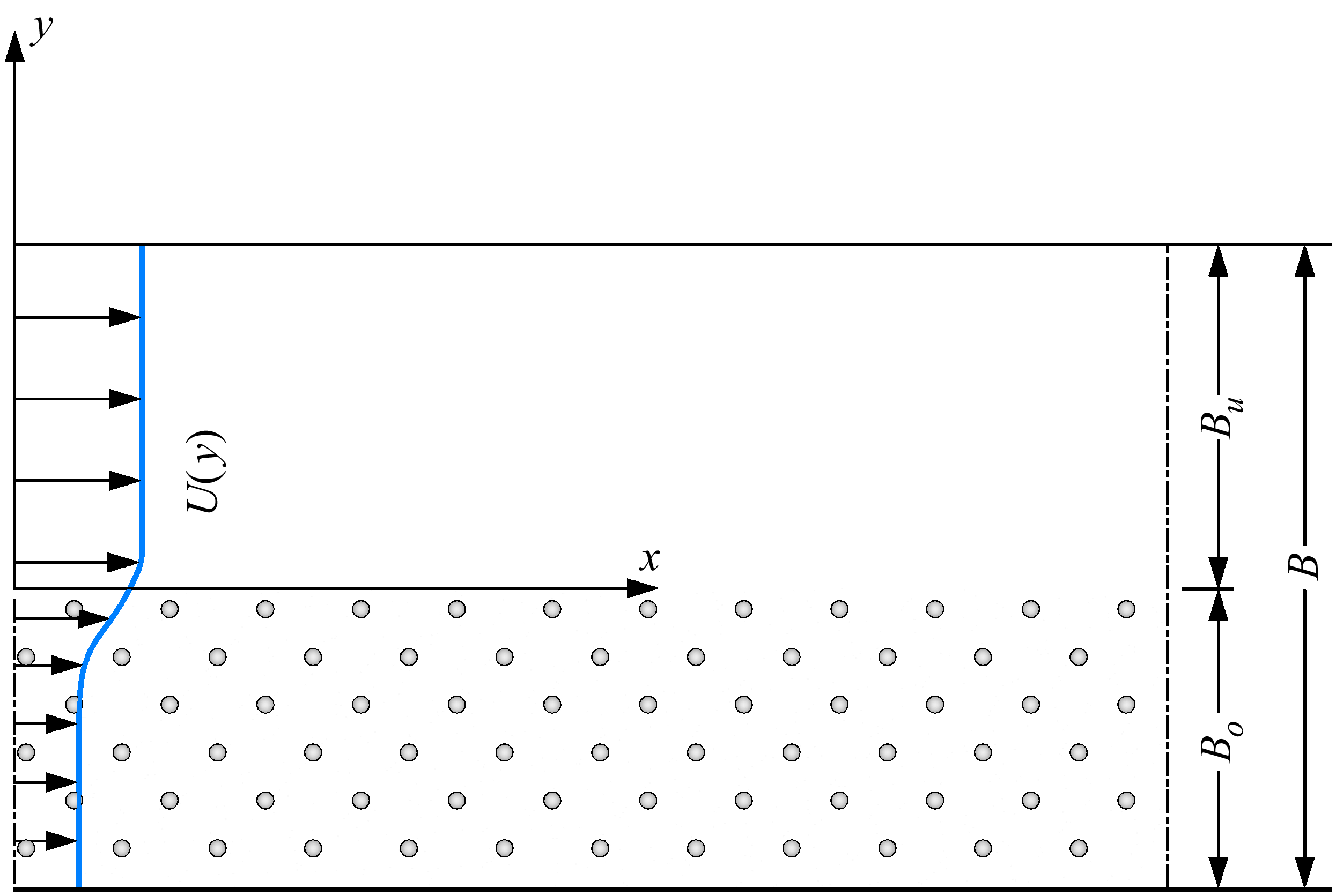
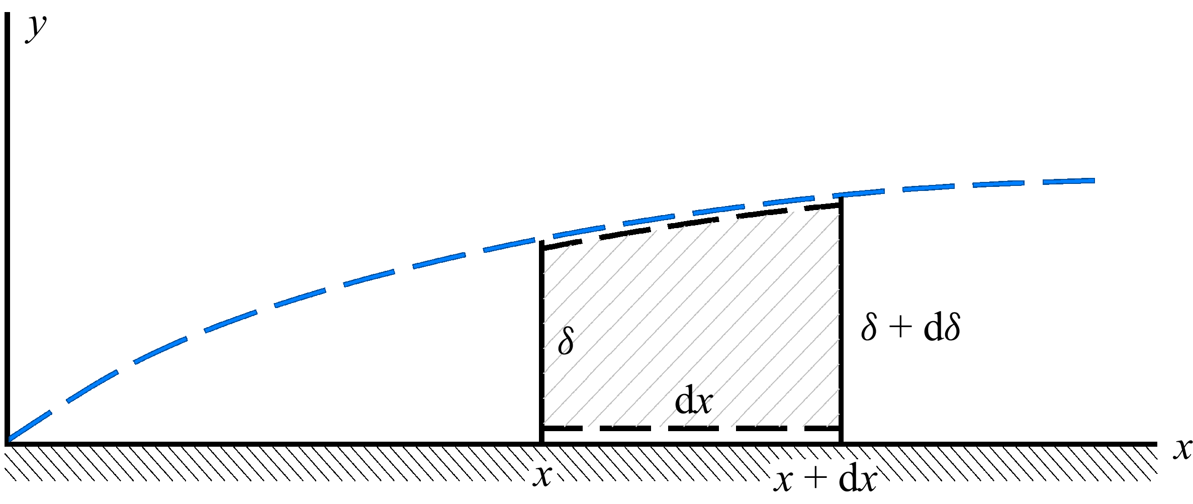
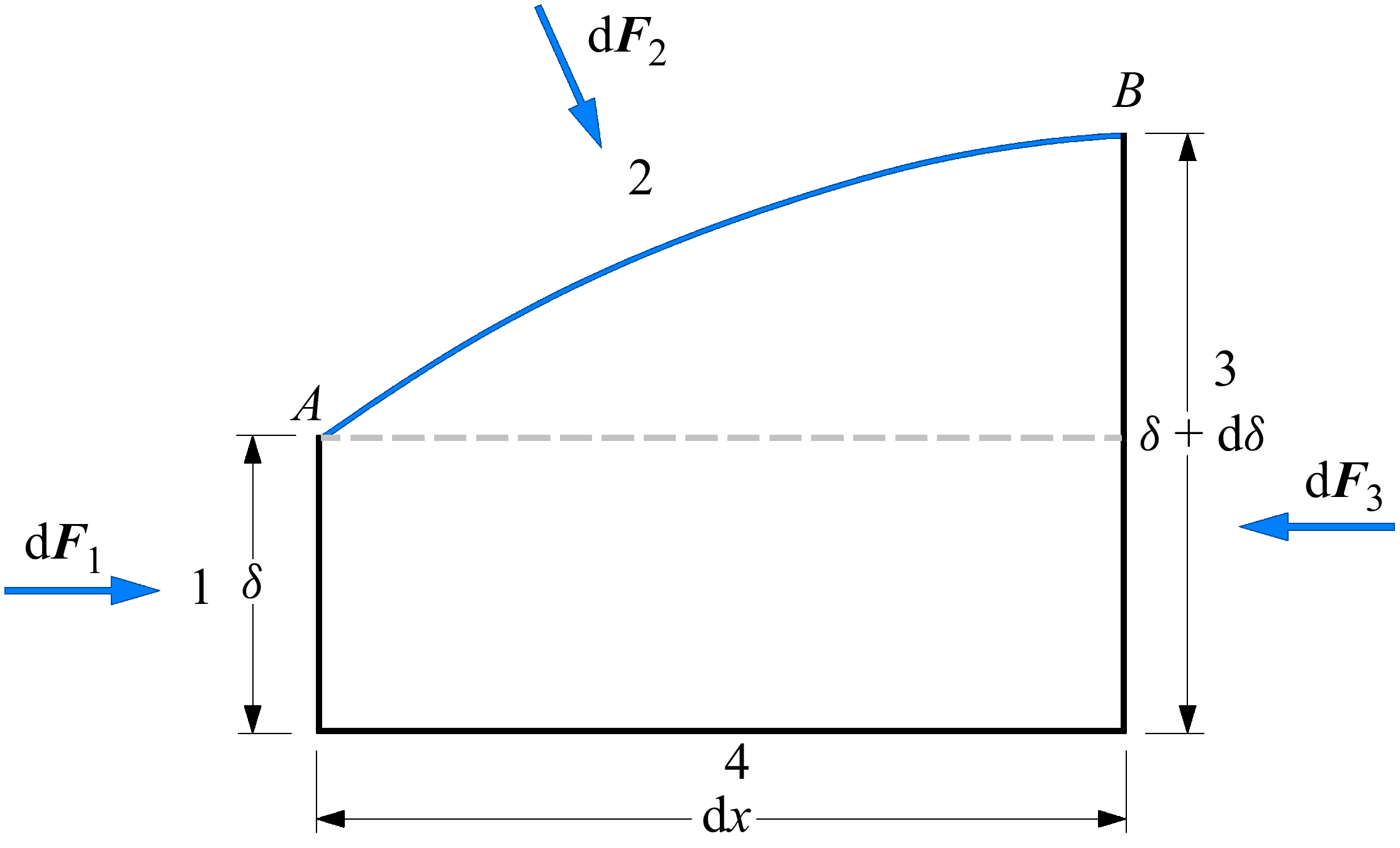
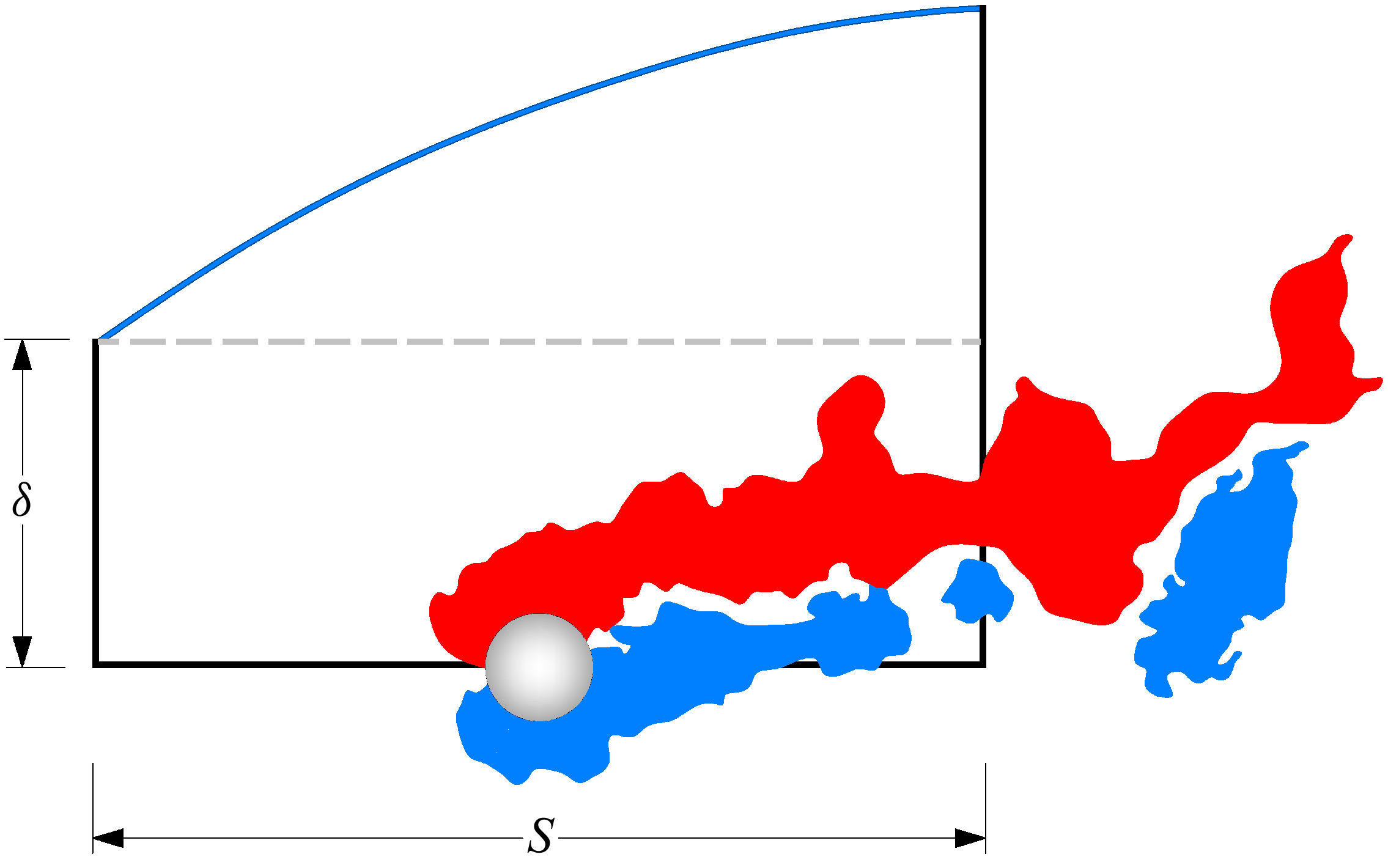

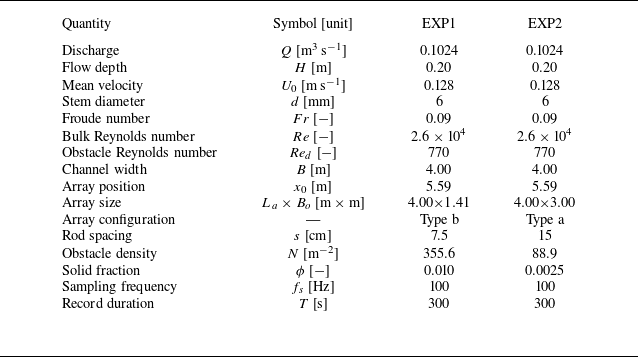

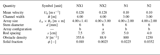
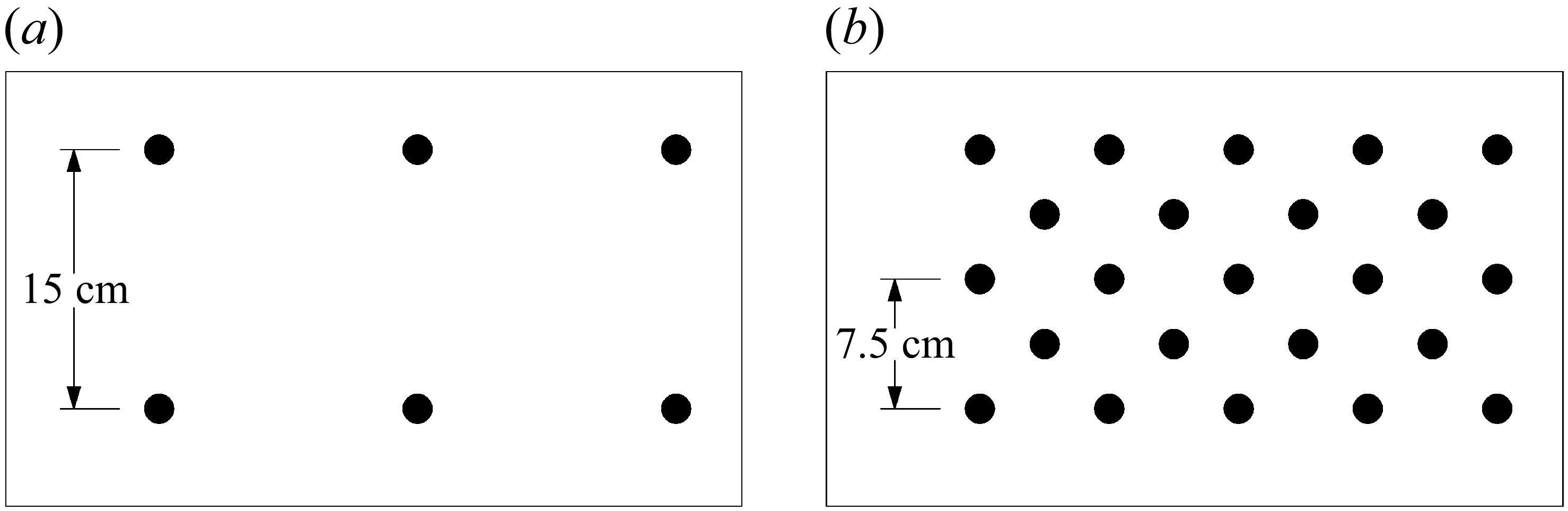
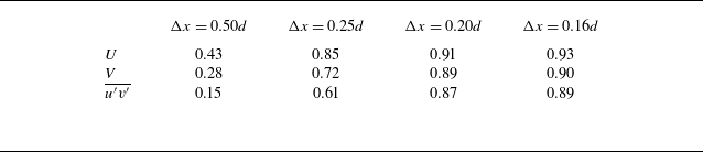
 Δx
 Iw

 Δx
 u′v′¯(x)

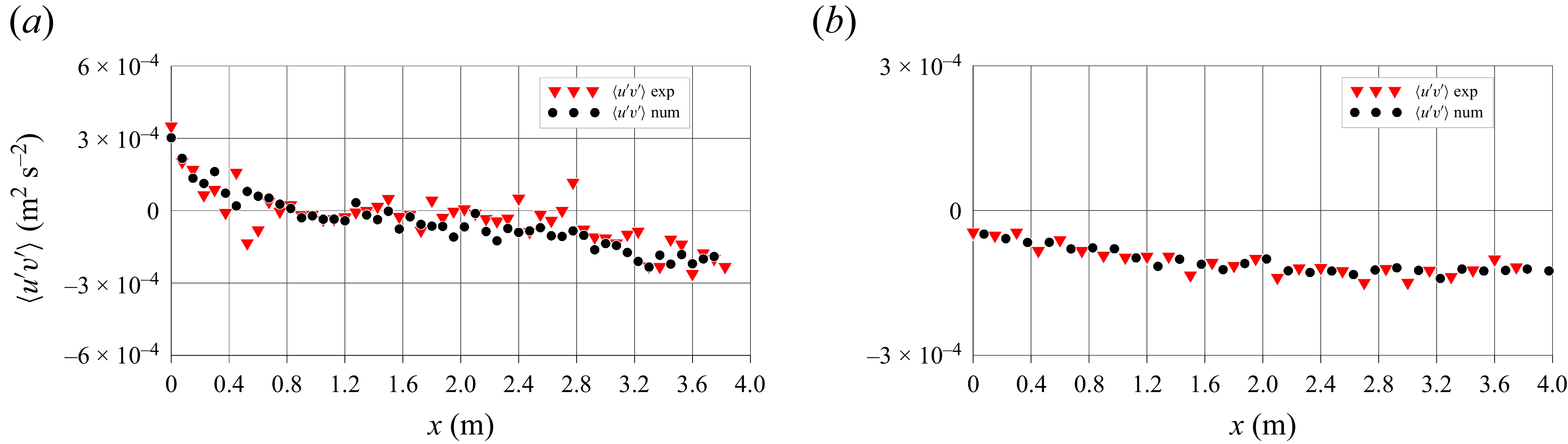
 u′v′¯

 y=0
 δ(x)

 ωz


 x
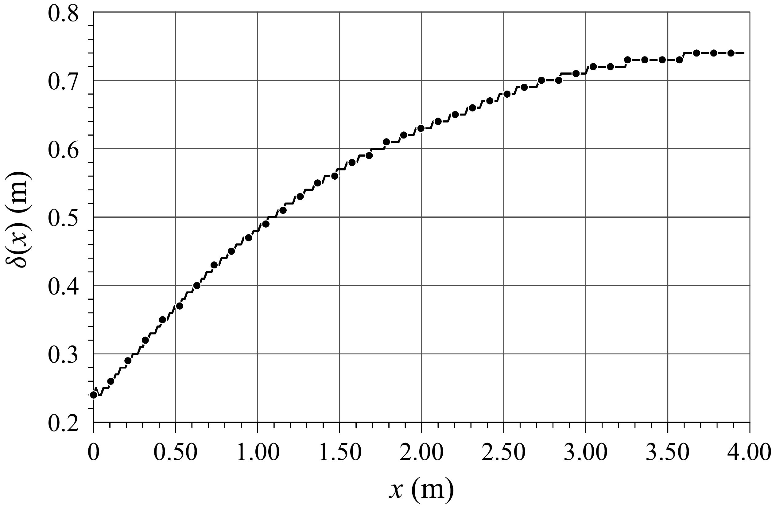
 δ(x)

 y=0
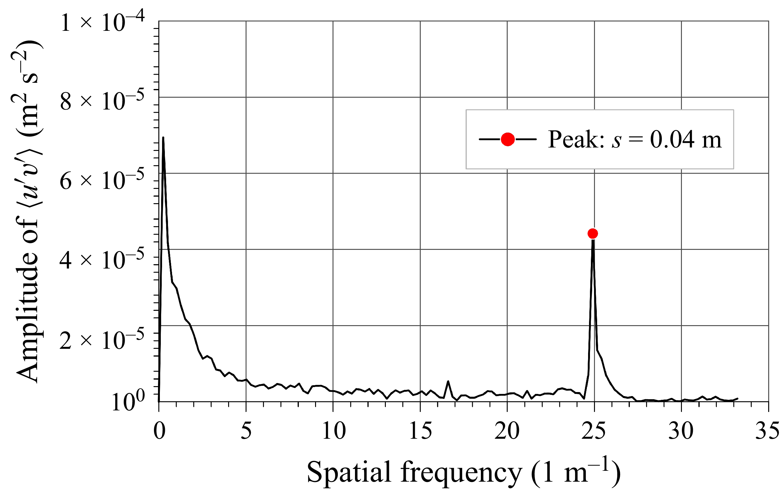
 u′v′¯
 x


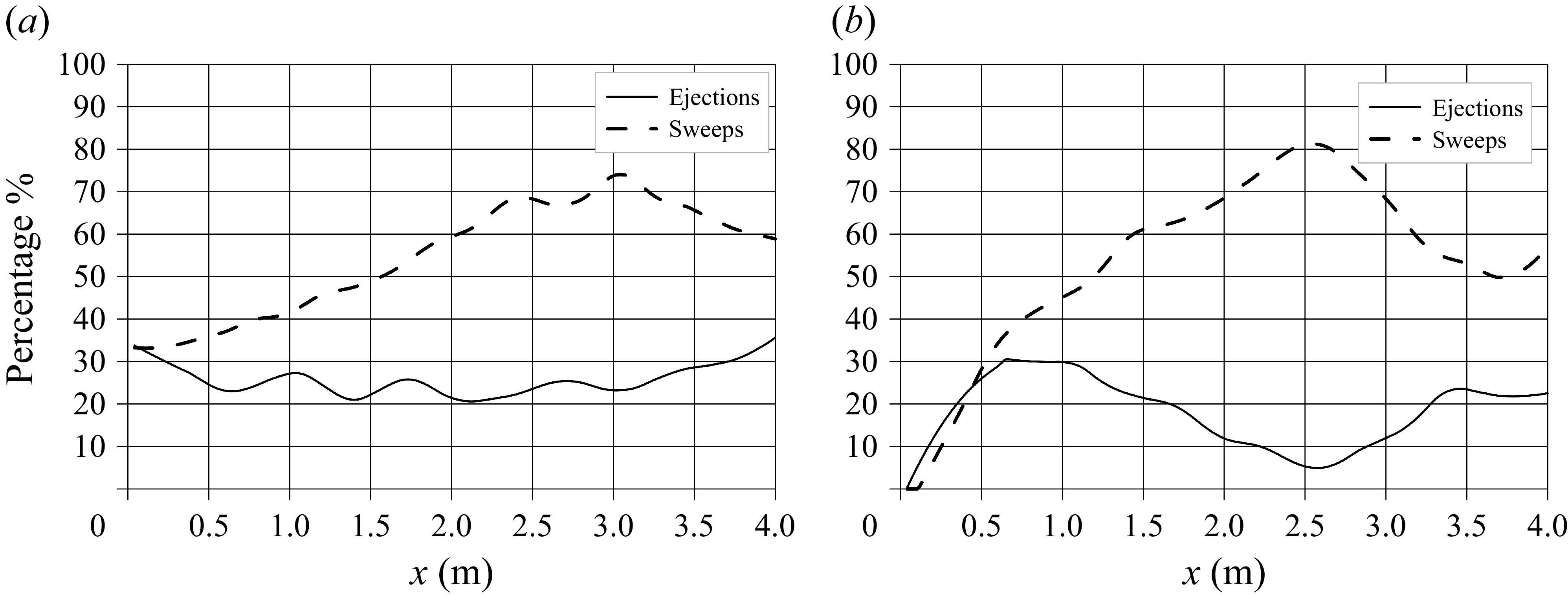

 H=1

 ⟨u′|ϕ⟩
 ⟨v′|ϕ⟩
 ⟨u′v′|ϕ⟩

 (u′,v′)
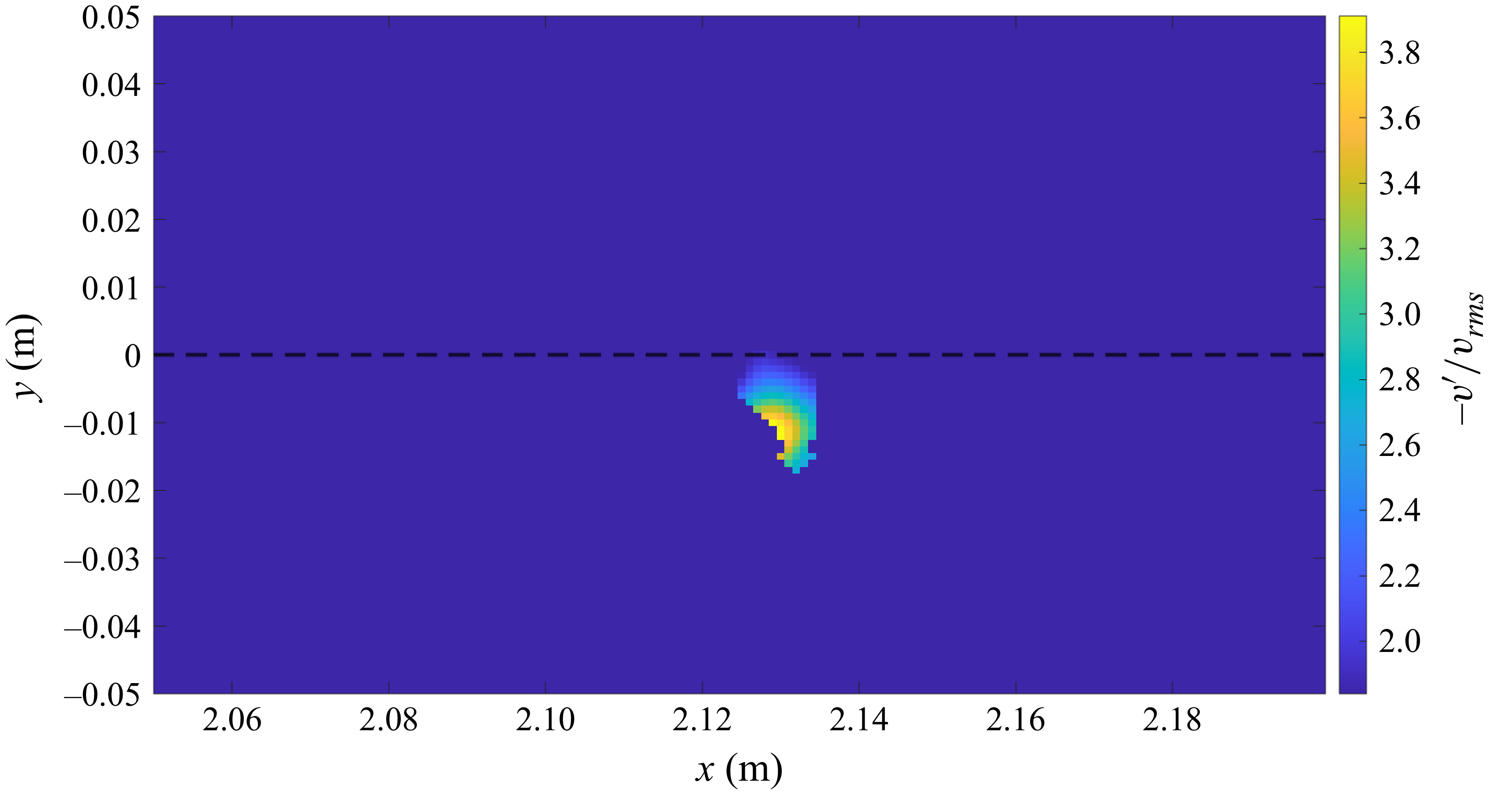
 −v′/vrms
 y=0
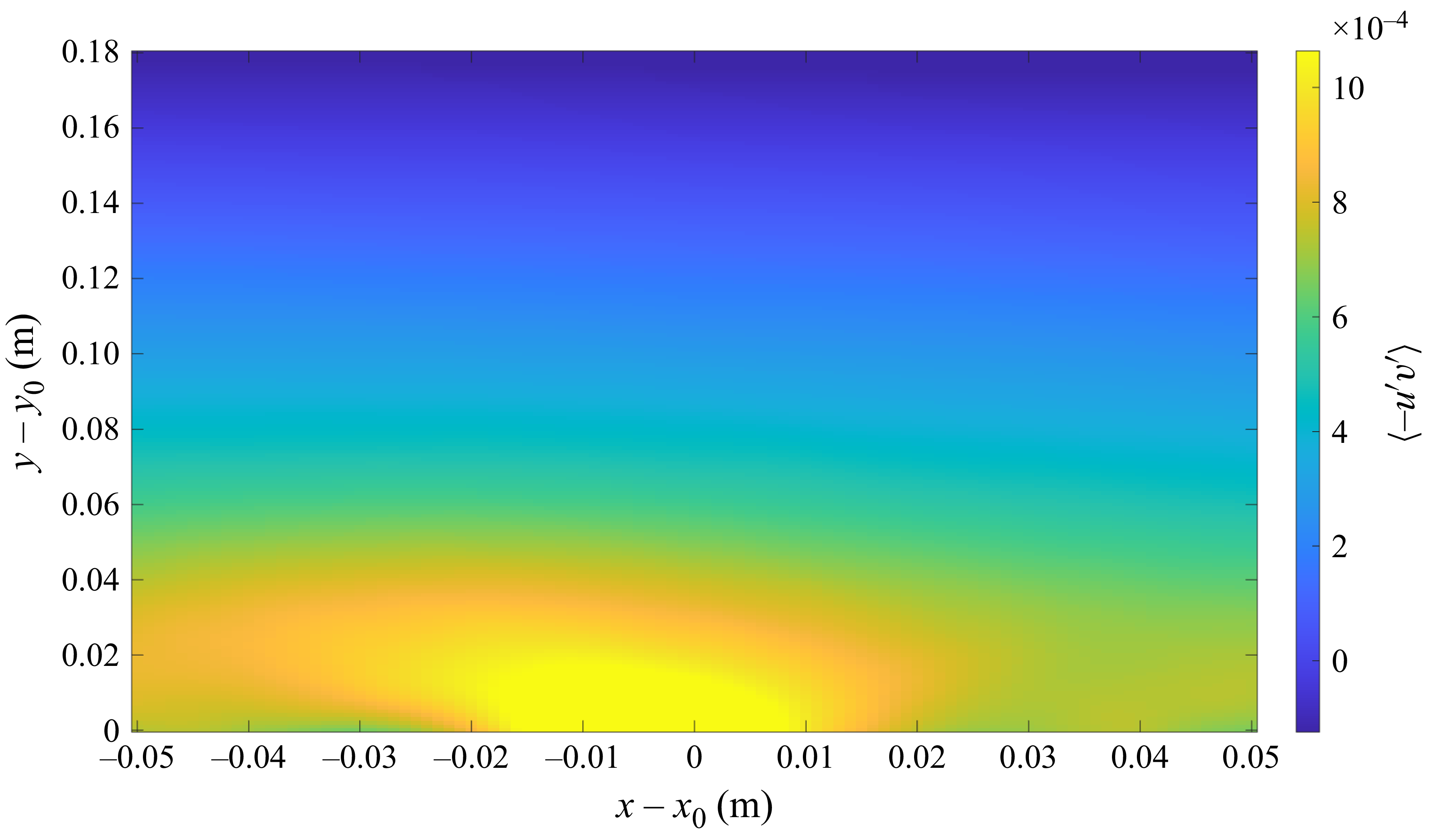
 −⟨u′v′⟩
 (x0,y0)

 λci
 y=0

 A2(t)
 y≈0
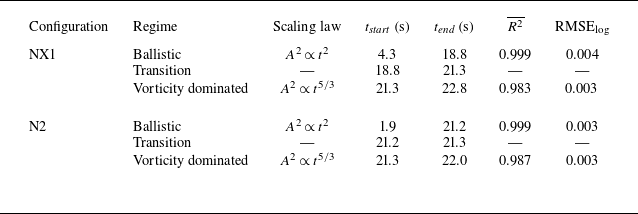
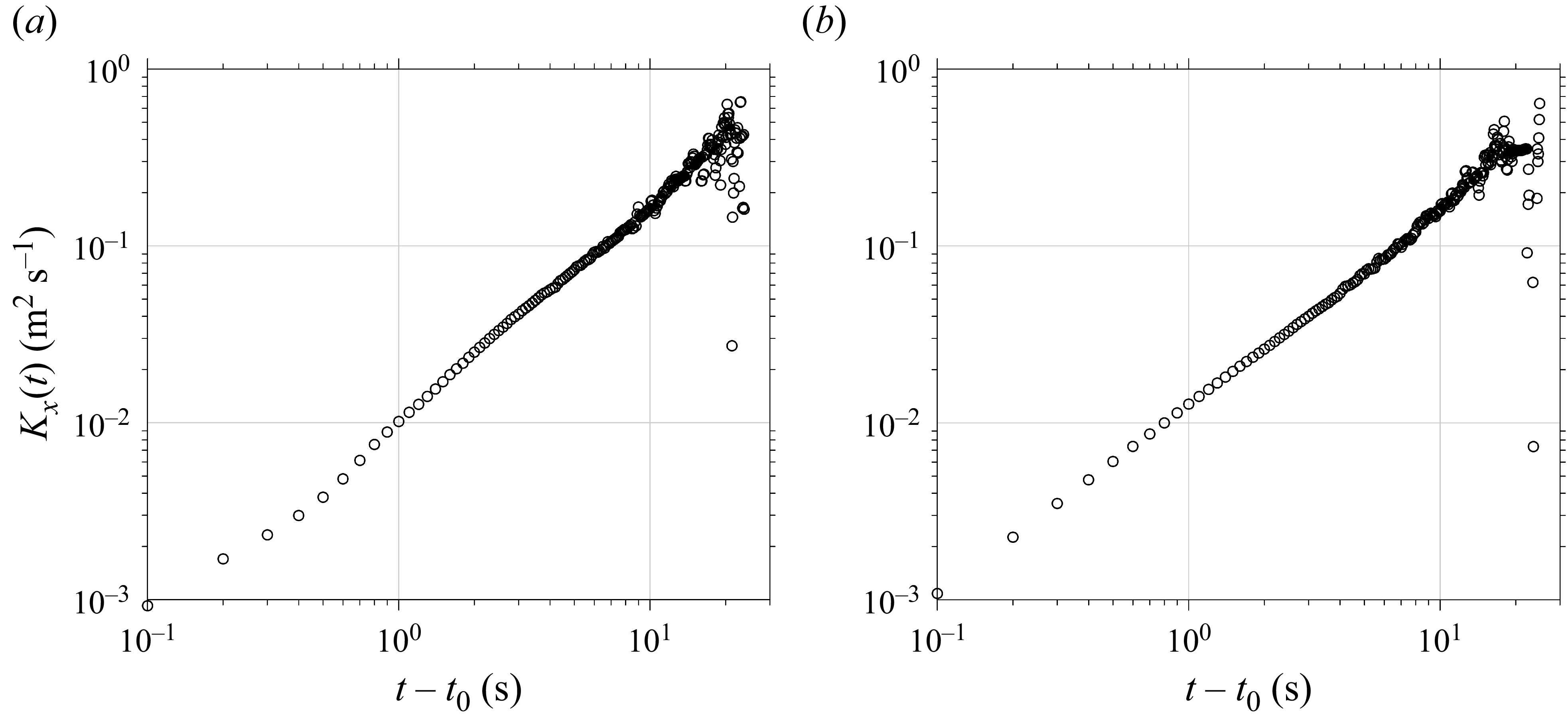
 Kx
 y≈0
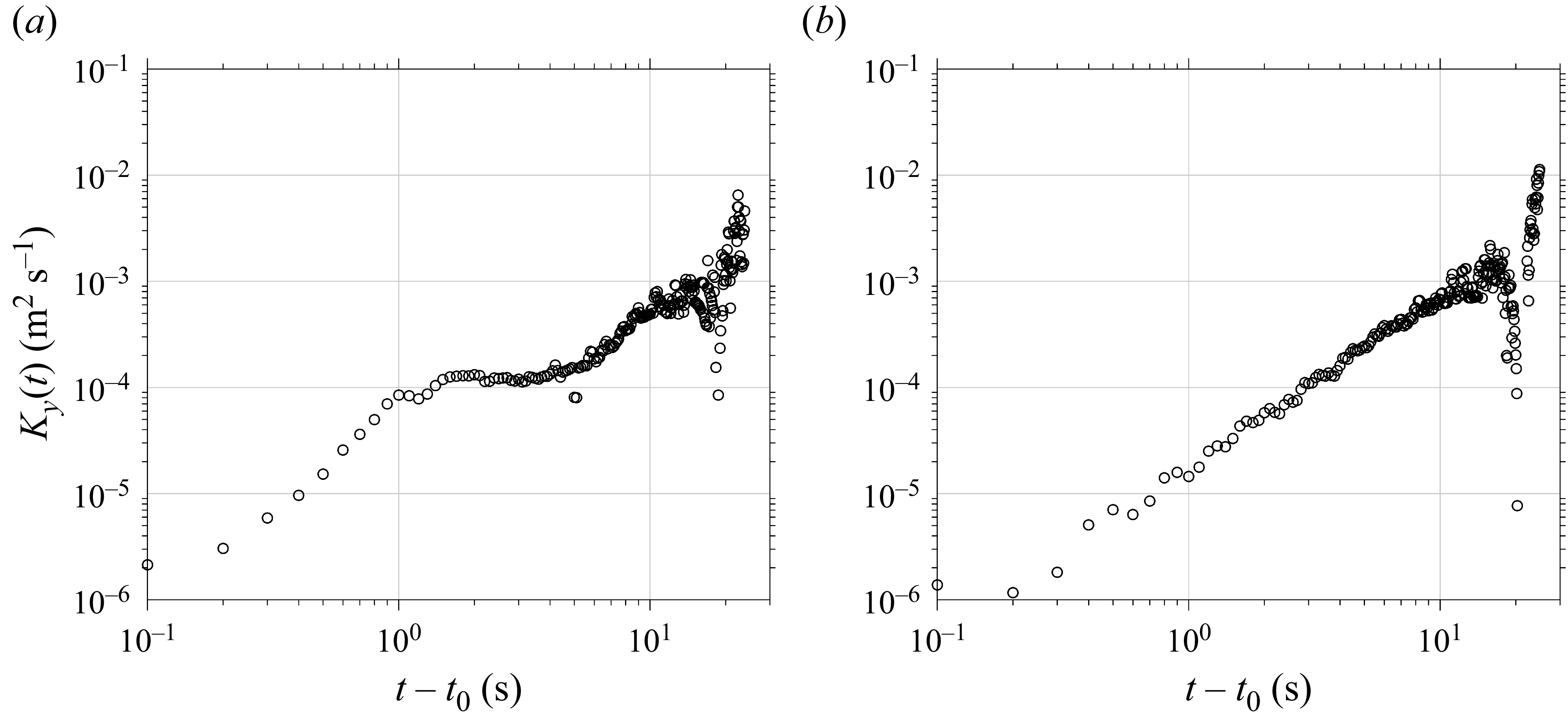
 Ky
 y≈0
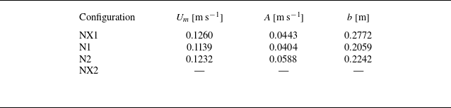
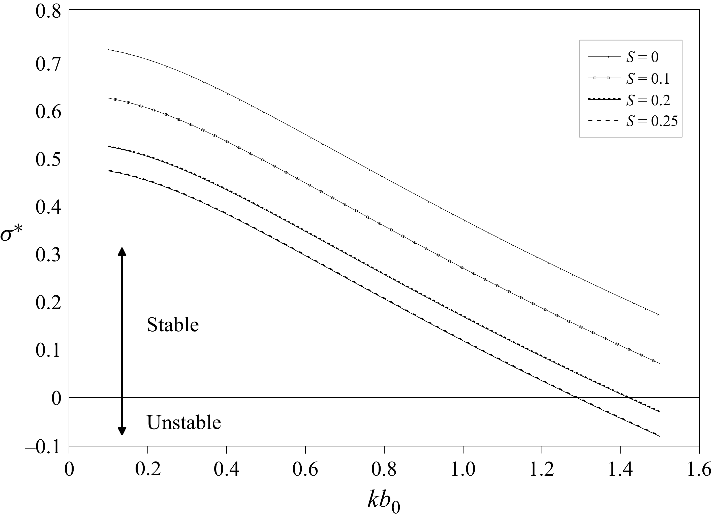
 σ∗(k)
 S
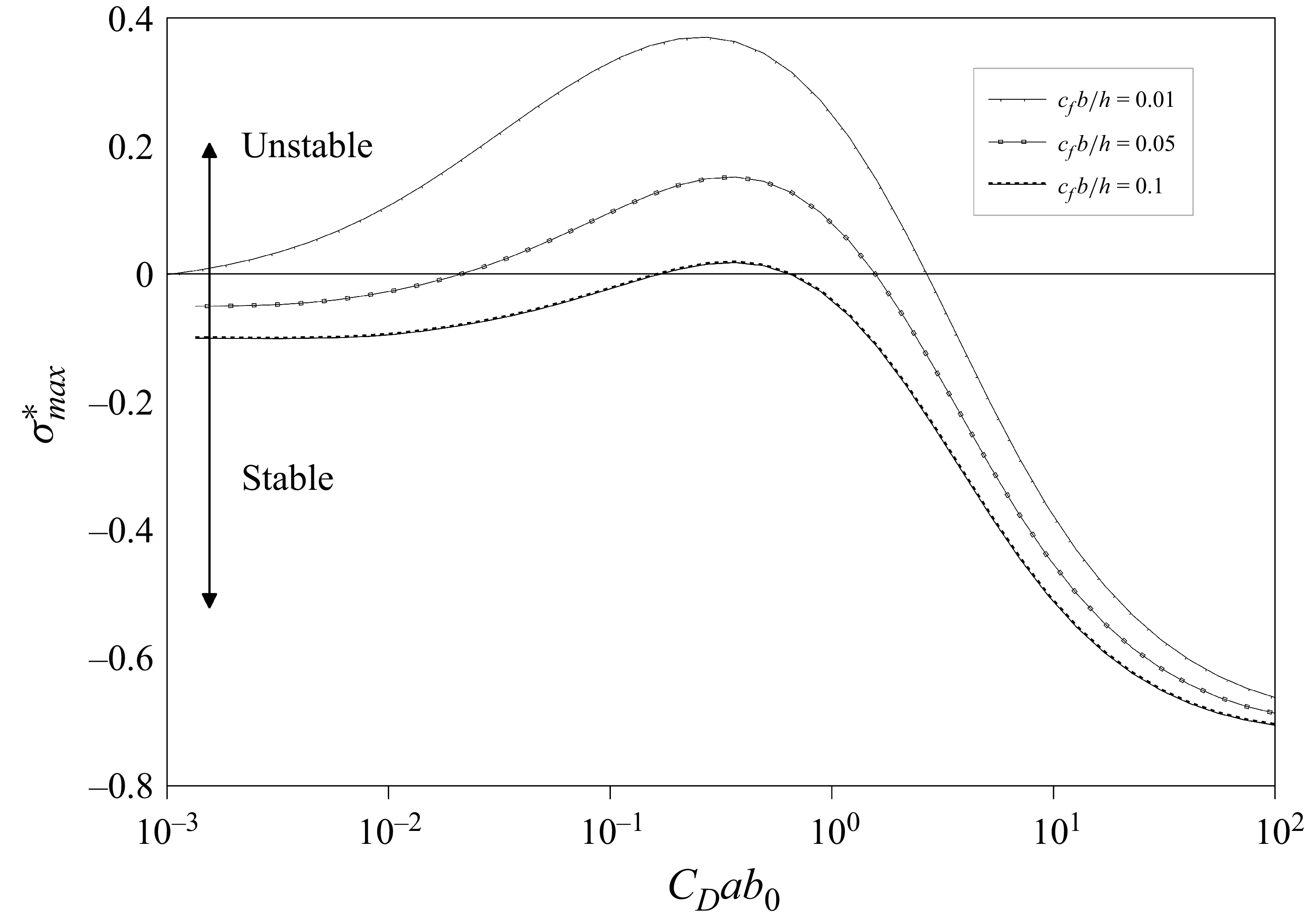
 σmax∗
 CDab0
 cfb0/h
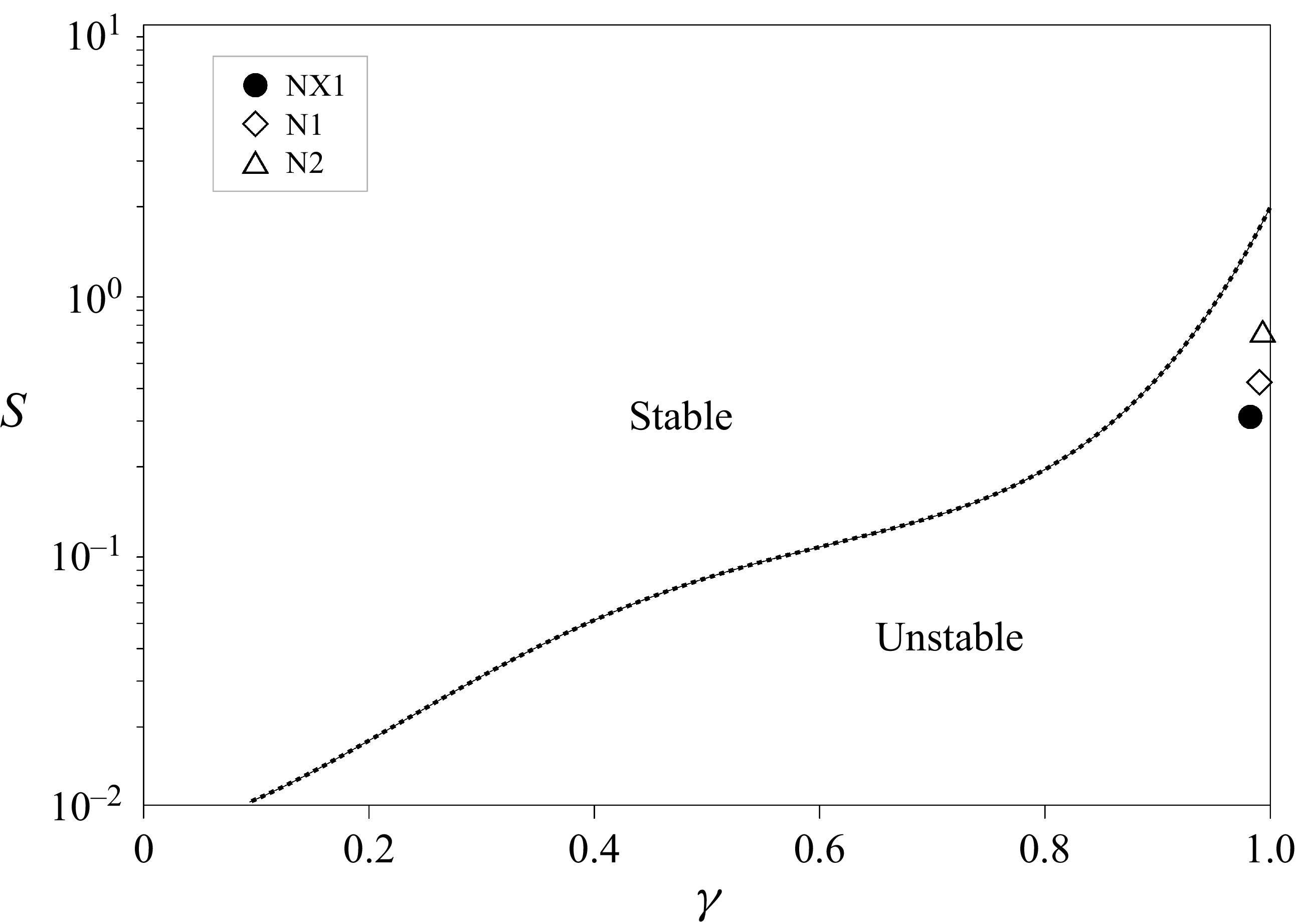
 (S,γ)
 (S,γ)
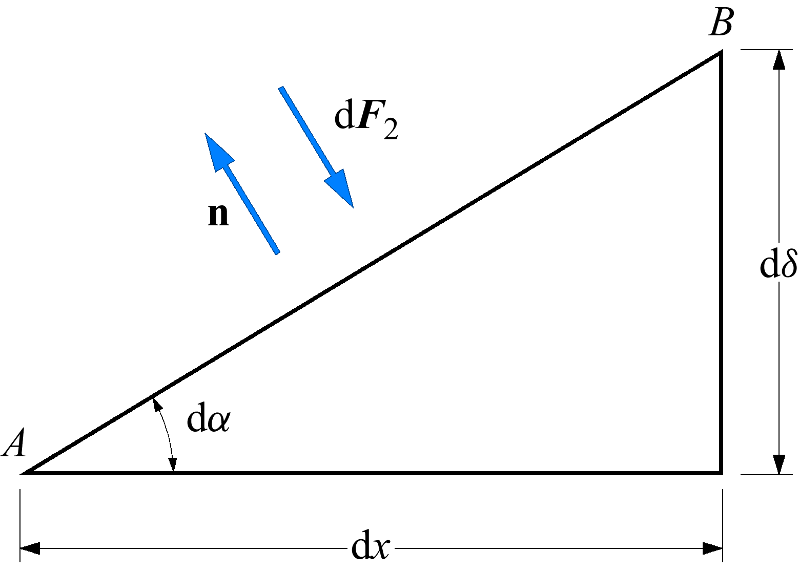
 AB


