The Indian economy experienced low productivity growth for much of the late nineteenth and twentieth century up to independence in 1947. Between 1890 and 1910 total factor productivity grew by only 0.4 percent per year as estimated by Stephen Broadberry and Bishnupriya Gupta (2010). Agriculture was the main culprit because it accounted for more than 70 percent of the economy. But, even modern sectors such as cotton textiles had low productivity compared to industrial countries such as the United States and Britain (Clark 1988; Clark and Wolcott 1999; Gupta 2011). Such poor productivity estimates match the disappointing income performance of the Indian economy in the colonial period (Madisson 2003; Roy 2010). Even in the decades before World War I when the economy performed better than in periods before or after, income per capita increased by only 0.6 percent per year from 1870 to 1913. Was poor productivity a hallmark of the colonial Indian economy?
Our article revisits this question of Indian productivity by focusing on railways, the key infrastructure investment made by the British Raj. An important modern sector of the colonial economy, railways employed 0.32 percent of total workers, 1.1 percent of nonagricultural workers, and accounted for 3 percent of GDP by 1911.Footnote 1 While economists find large social savings from railways, historians remain skeptical arguing that railways were developed to benefit colonial interests and did not lead to rapid economic growth.Footnote 2 Both sides of the literature are largely silent on the issue of productivity. The omission is important because if railways somehow failed the Indian economy, then low productivity could be a key reason. Indeed from the 1970s until the 2000s, low productivity has been identified as one of the problems for Indian railways (Alivelu 2010).
We shed new light on this debate by estimating total factor productivity (TFP) for Indian railways and by assessing its contribution to national income growth from 1874 to 1912. We use detailed railway system-level data drawn from official reports. Our sample includes the principal standard and meter gauge railway systems, and accounts for 95 percent of total output. Traditional approaches to estimating TFP often suffer from endogeneity problems because unobserved productivity shocks may be correlated with input choices. To circumvent this problem, we rely on the James Levinsohn and Amil Petrin (2003) production function estimator, which uses intermediate inputs such as fuel to address endogeneity concerns. We aggregate our railway TFP estimates into an industry TFP estimate using individual railway output shares as weights.
Unlike the overall Indian economy, we find evidence of significant productivity growth in railways. TFP increased at an average annual growth rate of 2.3 percent per year from 1874 to 1912. TFP growth was especially high in the period from 1900 to 1912 growing at an average rate of more than 3 percent per year. Railway TFP growth outpaced most Indian sectors. Moreover, Indian railway TFP growth was similar to or higher than railways in developed economies like the United States, Britain, and Spain. The international comparison is especially striking because labor productivity in Indian textiles, another key industrial sector, was amongst the lowest in the world circa 1900. If there was any development failure caused by Indian railways, it was not due to low productivity.
Our calculations also show that productivity growth in railways was a key driver of Indian economic growth. Higher TFP contributed 0.7 percent per year to Indian income per capita, which compounded over a 38 year period from 1874 to 1912 suggests social savings of 2.7 percent. Our sample period does not include the 1850s and 1860s, the first two decades of railway development, and hence our estimates capture the gains from productivity advances after railways largely displaced other modes of transportation. Nevertheless we find a nontrivial proportion of the gains from railways came from productivity growth after their introduction in India.
What explains the strong productivity performance of colonial railways? We examine three potential explanations. First, we study reallocation effects, including entry, exit, and changes in market share, and find that they explain only a limited portion of industry TFP growth. Second, we find that greater capacity utilization accounts for a small share of total TFP growth. To assess the quantitative significance of capacity utilization, we modify the production function estimation to include utilization variables, such as train miles run per track mile. The adjusted TFP estimates are 76 percent of the original estimates. Third, we investigate the role of technology adoption. Drawing on data from the 1900s, we find that many major technologies emphasized by contemporaries, such as interlocking signal stations, were adopted in increasing numbers by 1912. We also find that technology adoption variables can explain some of the variation in TFP across and within railways over time. The remaining TFP growth appears to be related to undocumented technological changes and improved governance and regulation led by the Government of India.
We begin by describing India's railway development and then lay out our data sources. Section 4 discusses how we estimate TFP and section 5 presents the results. We estimate the impact of TFP growth on income per capita in section 6 and explore potential explanations to account for the surprisingly high rate of TFP growth in section 7.
BACKGROUND ON INDIAN RAILWAYS
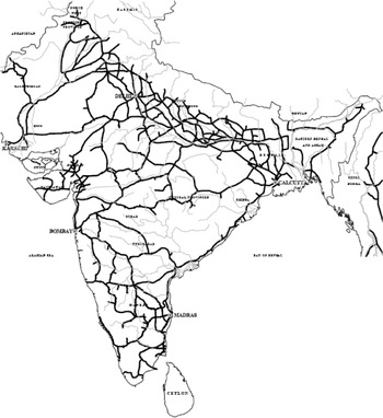
After the first passenger line opened in 1853, the subsequent development of the rail network was rapid especially in the 1880s and 1890s. By the early twentieth century, India had the fourth largest rail network in the world. It was of similar or greater size than Brazil, China, and Japan, but smaller than the Unites States. The initial network was constructed on a broad gauge (5 feet 6 inches) and consisted of trunk lines connecting the major ports of Bombay, Calcutta, Karachi, and Madras to the interior. Subsequent lines broke from the standard gauge and were constructed on a cheaper meter gauge (3 feet 3 ¾ inches). These lines often served as feeder lines connecting to the main trunk route. A few narrow gauge lines of less than 3 feet were also constructed connecting to different hill stations, but they carried less than 1 percent of the overall traffic. While economic and military concerns dictated route placement in the earlier decades (Thorner 1955), social concerns following the devastating famines of the 1870s led to the construction of some protective famine lines in the 1880s. Figure 1 displays the rail and river network as of 1909.
Private British companies managed the initial construction and operation of the lines. These companies received a 5 percent dividend guarantee on invested capital. Railways operated under concession contracts with the Secretary of State, a cabinet member of the British government. The Government of India (GOI) enforced the contracts and regulated railway companies. The largest and most important of the early railway companies were the East Indian Railway and the Great Indian Peninsula Railway. The East Indian served Calcutta and was constructed in the 1850s. The Great Indian Peninsula Railway served Bombay beginning in the 1850s. Jointly these two railway companies accounted for over 50 percent of all traffic in the 1870s.
There was a shift in ownership and operation beginning in the 1870s when the GOI began to construct and manage new railway lines. A few Princely States also entered the field during this time directly managing lines or outsourcing the operations to private companies. The period was short-lived and in the 1880s a hybrid GOI owned but privately operated structure emerged. The GOI owned a majority of the capital and private companies operated the railway under a concession contract for 25 years. The profits were split between the GOI and the company in proportion to their capital. The dividend guarantee was retained, but lowered significantly from 5 percent to 3 or 4 percent. The public-private partnership model was the dominant organization form in Indian railways until the 1920s when complete nationalization was gradually introduced.Footnote 3
MAP OF INDIAN RAILWAYS IN 1909

Although capital expenditures per mile were high in the first wave of construction, they declined in our period of study as the GOI became a majority owner of the lines and the cheaper meter-wide gauge lines were constructed (Bogart and Chaudhary 2012b). Passenger and freight traffic also increased significantly in this period, growing at comparable rates with freight accounting for almost 65 percent of total revenues. While net returns on railways were below 5 percent in the 1860s and 1870s, they increased to over 5 percent in the 1880s and averaged over 6 percent by 1913. Thus, our period of study is an important one encompassing the construction of the second generation of railway lines, the partial nationalization of the network, and an increase in returns over the guarantees.
The literature has generally viewed British railway companies operating in India with a high degree of skepticism. John Hurd (2007) argues that railways missed opportunities for development and that management was often complacent. Stuart Sweeney (2011) highlights the revolving door between the public and private sector in this period when many public regulators joined the boards of private railway companies after retiring from service. This critique of railways fits into a larger picture of an unproductive Indian economy constrained by colonial polices and unable to achieve economic growth. But, in our view railway performance has not been assessed by any clear metric. Much of the evidence relies on qualitative arguments on the negative effects of public guarantees. Rarely is the productivity of Indian railways even considered. Our article provides a fresh quantitative perspective by estimating TFP growth using consistent series on capital, labor and fuel for a large sample of railways.Footnote 4
DATA
We construct a new data set of Indian railways from 1874 to 1912 using the Administration Reports on the Railways in India, published annually from 1884, and the Report to the Secretary of State for India in Council on Railways in India, published annually from 1860 to 1883. Many key variables necessary to estimate productivity are not reported in the earlier publications. Hence, we begin our analysis in 1874 when the reports begin publishing consistent series on capital, output, labor, and fuel, and we end our analysis just before World War I. Although the reports are detailed, the data series often present numerous challenges that we describe below beginning with the unit of observation.
Our sample follows all the major standard and meter gauge railways operating between 1874 and 1912 including those that go on to merge with another railway.Footnote 5 The unit of observation is a railway or a railway system, which includes the primary railway line and any secondary lines operated by the system that are owned by either the Princely States, the GOI, or private companies.Footnote 6 A majority of the mileage within a system belongs to the primary line and all the lines within a system are generally of the same gauge though a few systems begin to operate a small mileage of narrow gauge lines (2 feet) in the 1900s. The published input and output series are not always consistent in how they report railway systems so we adjusted the capital, labor, and fuel series to match precisely the railway-system unit of the output series.Footnote 7 In a few cases, we could not precisely match the series because labor was reported for the entire railway system including the narrow gauge lines and output was reported only for the standard or meter gauge portion of the system and not the narrow gauge.Footnote 8
We measure output using a weighted average of ton-miles and passenger-miles.Footnote 9 Following Douglas W. Caves, Laurits R. Christensen, and Joseph A. Swanson (1980), the weights are defined using the cost elasticity of ton-miles and passenger-miles. Based on cost elasticity estimates from an earlier study (Bogart and Chaudhary 2012a), we assign a weight of 0.56 to ton-miles and a weight of 0.44 to passenger-miles. On the input side, we use total employees as our measure of labor. The labor series are also disaggregated by race into Europeans, Anglo-Indians, and native Indians. Although Indians represented over 95 percent of total workers on average, the small number of Europeans dominated the high-skilled jobs of managers and engine drivers, while Indians dominated the lower-skilled jobs. Disaggregation by race does not affect the results.
The fuel series is our most challenging one because it needs to account for changes in quality. Most railways shifted from British coal and wood to Indian coal between 1874 and 1912. Wood yielded less British thermal units (BTU) per ton than British coal, but Indian coal was also less efficient than British coal. One ton yielded 80 to 90 percent as much BTU as one ton of British coal. Unfortunately, the reports do not consistently list fuel consumption by type. We use this information in the years it is available to construct a quality-adjusted measure of fuel, which is reported in terms of Indian Kurharbaree coal (the main fuel source of the East Indian Railway).
From 1890 to 1901 we have information on total fuel consumption in tons of Kurharbaree coal for each railway. Between 1897 and 1901 the reports are very detailed and give the conversion rate from Indian coal, foreign coal, and wood to Kurharbaree coal for each railway. Beginning in 1902 the reports only list the tons of Indian coal, foreign coal, and wood consumed by each railway. To convert the 1902 to 1912 series into tons of Kurharbaree coal, we apply the 1901 conversion rates (or 1900 if unavailable). We use a similar approach for 1874 to 1881.Footnote 10
The years from 1882 to 1889 are the most challenging because we only have information on total tons of fuel consumed. We use a three-step procedure in this period. First, we calculate a fuel quality adjustment factor for 1881 and 1890, the nearest years for which we have detailed information on fuel type.Footnote 11 Second, we linearly interpolate the quality adjustment factor between 1881 and 1890. Third, we multiply the quality adjustment factor with the total tons of fuel consumed to get an estimate of the tons of Kurharbaree coal consumed by each railway.Footnote 12
Our final input series is capital which includes track miles, locomotive engines, vehicles, stations, warehouses, bridges, and stores of other equipment. Using the published capital series, we first compile nominal capital outlay on each railway system in each year, which includes the cumulative value of all past investments (i.e., new track, vehicles, etc.) minus retirements.Footnote 13 Our main concern with the nominal series is the implicit assumption of a constant price deflator for investment. To address this problem, we begin by taking the yearly difference in the capital outlay series to get an estimate of nominal investment less depreciation.Footnote 14 We then construct a real investment series by multiplying nominal investment with a capital price deflator based on wages for unskilled labor and prices of British capital imports.Footnote 15 Finally, we construct a capital stock measure for each railway using the perpetual inventory method, which adds yearly real investment to the previous years’ capital stock. Based on our newly constructed series, we believe the capital outlay series reported in the official publications probably under states the capital stock. Aggregating across all railways in 1874 our newly constructed capital series is 17 percent higher than the reported capital outlay. Our estimates differ from the reported capital outlay because wages and the price of railway capital imports were lower in nominal terms in the 1850s and 1860s when the first trunk lines were built.
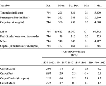
Table 1 summarizes the variables used in the productivity analysis. The average railway transported 291 million ton-miles and 325 million passenger-miles. In terms of inputs, the average Indian railway employed fewer than 16,000 employees, consumed 79,000 tons of fuel in terms of Kurharbaree coal, and had 948 miles of track. The average capital stock was 137 million rupees. It is also worth noting the tremendous variation across railways and over time as captured by the standard deviation. The largest of all railways, the East Indian, averaged 857 million ton-miles and 679 million passenger-miles.
SUMMARY STATISTICS

Sources:
Administration Reports on Railways in India, 1874 to 1912.
The raw data also provide immediate clues on the rate of productivity growth for Indian railways. The bottom of Table 1 shows the output weighted average of labor, fuel, and capital productivity growth disaggregated by time period. There was a large increase in both output per worker and output per capital in the railway sector with annual growth rates of 2 percent and 3 percent respectively. The other measures of capital namely miles also show evidence of productivity growth. Fuel productivity growth is relatively slow and even turns negative in the 1890s. Overall, the partial productivity measures suggest we should find TFP growth in Indian railways.
METHODOLOGY
The productivity literature proposes several methods to estimate TFP and TFP growth (Van Biesebroeck 2008). The Index Number (IN) method is the standard approach. It calculates the difference between output growth and a weighted average of the growth of inputs. The weights are the share of total costs paid to each input including labor, capital, and fuel. The IN method is problematic in our setting because cost shares are not directly observable. The reports indicate that working expenses equaled 45 percent of total revenues on average from 1882 to 1912, implying that 55 percent of revenues were paid to capital. Unfortunately, there is no information indicating what proportion of the remaining 45 percent of revenues went to labor versus fuel. Evidence from the East Indian Railway suggests that labor costs were around two-thirds of all working expenses (Derbyshire 1987). Extrapolating from this example implies that capital's cost share was 0.55, labor 0.3, and fuel 0.15. The previous costs shares are not unreasonable as they are in line with other historical studies on railway productivity.Footnote 16 Nevertheless, we do not want to rely solely on data from the East Indian Railway.
Parametric estimation of TFP is another method and one that is well suited to our data. The goal in this approach is to estimate the elasticity of labor, capital, and fuel assuming a form for the production function. In the Cobb-Douglas case, the estimating equation is

where yit is the natural log of output for railway i in year t, lit, kit, and mit are the log of labor, capital, and fuel respectively, and εit is the error term. The main challenge in this approach is to obtain unbiased estimates of the elasticities on labor, capital, and fuel. The standard Ordinary Least Squares (OLS) estimates are likely to be biased because input choices may depend on unobserved productivity shocks. To illustrate the problem, we can rewrite the error term as εit =ωit + ∊it where ωit is a state variable for productivity known to the railway manager and ∊it is a shock to productivity but is unobserved by the manager. Because productivity is a complement to inputs like labor, the railway manager will adjust its input choices depending on ωit (see Griliches and Mareisse 1998).
There are several alternatives addressing this endogeneity problem. The most straightforward is to introduce fixed effects (FE) when panel data are available. However, the FE approach only exploits within-firm variation, so researchers have also proposed alternative estimators. The Levinsohn and Petrin (LP 2003) estimator uses reasonable assumptions about the evolution of capital and use of intermediate inputs. LP assumes that the capital stock is determined by the previous period's investment decision and hence is uncorrelated with unobserved productivity shocks in the current period. LP also assumes that intermediate inputs chosen in the previous period are uncorrelated with unobserved productivity shocks in the current period. The LP method is appropriate for our setting because railway capital clearly evolved from investment decisions made in prior years. We also have a consistent series on fuel, the intermediate input, and the amount of fuel in year t is plausibly independent of shocks in previous years.Footnote 17
After estimating the parameters in equation 1 using OLS, FE, or LP, we estimate the log of individual railway TFP using the following equation

where â′s are the estimated parameters. As a final step, the log of industry TFP is calculated as the output weighted average of individual railway TFP measures. Let θit be the share in total output for railway i in year t and let n be the number of railways. The natural log of industry TFP in year t is given by the formula

RESULTS: TFP ESTIMATES
Industry TFP
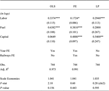
We first review the production function coefficients on capital, labor, and fuel across the three estimation techniques in Table 2. Specification 1 is the standard OLS model, a Cobb-Douglas production function augmented by year FE, specification 2 includes railway FE, and specification 3 reports the Levinsohn-Petrin (LP) estimates. While the coefficients on labor are somewhat similar across the different methods, the coefficients on capital and fuel are very different. Similar to the original Levinsohn and Petrin (2003) study, we find the LP estimates on capital are higher than OLS suggesting the latter generates a downward bias on capital elasticity. The OLS estimates on fuel and labor appear to be biased upwards because they are significantly larger than the LP estimates. In the rest of the discussion, we focus on the well-identified LP estimates.
COEFFICIENT ESTIMATES

* = Significant at the 10 percent level
** = Significant at the 5 percent level
*** = Significant at the 1 percent level
Notes:
Robust standard errors clustered at the railway level in parentheses in specifications 1 and 2. Bootstrapped standard errors in specification 3.
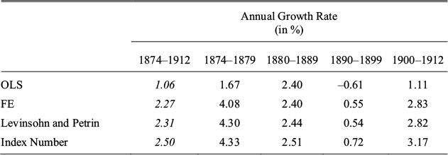
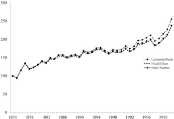
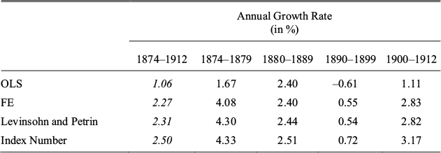
Table 3 reports the average annual growth rate of industry-level TFP by subperiod and method. The LP estimates suggest TFP increased at an annualized rate of 2.3 percent per year with most decades enjoying high productivity growth other than the 1890s. The other estimates also support the view that TFP growth was positive and rapid in the Indian railways sector between 1874 and 1912.
Figure 2 plots the industry-level TFP indices standardized to 100 in 1874 for IN, FE, and LP. The trends in TFP are remarkably similar despite differences in levels.Footnote 18 TFP was volatile in the late 1870s, increasing in 1877 and then decreasing by roughly the same amount in 1878. These fluctuations are linked to famines, which estimates suggest affected 58 million people spread over an area of 250,000 square miles between 1876 and 1878 (Government of India 1880). In general, railways were influenced by the macroeconomic climate of the country. Agricultural shocks probably account for the TFP dip in 1908, which was a bad harvest and trade year. There is a marked change in average TFP growth around 1900. It was stagnant in the 1890s averaging less than 0.5 percent per year, but in the 1900s TFP growth accelerated and was particularly high from 1903 to 1907 and from 1909 to 1912. In general, the early 1900s was a “golden age” for the productivity of Indian railways.
ESTIMATES OF TFP GROWTH RATES
Notes:
See the text.
Finally, we find no evidence of economies of scale. The F-statistic reported at the bottom of Table 2 shows that the sum of the input coefficients is never statistically different from one in any of the specifications. The absence of scale economies is noteworthy because many Indian railway systems more than doubled in size from the 1870s to the 1910s. However, consolidation and internal growth by themselves did not increase productive efficiency since economies of scale were limited.
Railways in Comparative Perspective
The existing literature is generally pessimistic about India's economic progress in the colonial period. For example, capital and labor productivity in cotton textiles remained unchanged between 1890–1894 and 1910–1914 (Clark and Wolcott 1999). Labor productivity in agriculture was unimpressive, growing at an average rate of 0.6 percent between 1870 and 1910 versus 1.6 percent in manufacturing and 0.5 percent in services (Broadberry and Gupta 2010). As noted in Table 1, labor productivity in railways increased by 2 percent per year on average over the same period and by 3.2 percent in the 1900s. Thus, railways were one of the most successful industries in India at this time.
TFP INDEX (1874 = 100)

Indian TFP growth is also impressive by international standards. Surprisingly, Indian railways had higher TFP growth than U.S. railways (2.1 percent), British railways (0.8 percent), and Spanish railways (1.5 percent) in the same period.Footnote 19 Moreover, these patterns are not an artifact of the choice of estimation strategy because even within the set of IN calculations, Indian TFP growth at 2.5 percent is above the United States and Britain. Thus the critical view of Indian railways in the literature is inconsistent with its productivity growth.
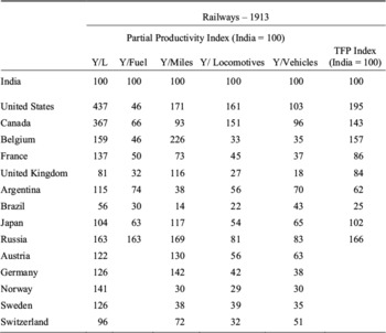
In terms of productivity levels, Indian railways were also comparable to many countries circa 1913. Table 4A shows railway output per employee, per ton of coal, per track mile, per locomotive, and per vehicle for a large set of countries around the world.Footnote 20 We convert ton-miles and passenger-miles into a single output measure using revenues weights for passenger and freight traffic in each country. Perhaps unsurprisingly labor productivity on Indian railways was below richer countries such as the United States and Canada. The United States, for example, had more than four times higher output per railway worker than India.
INDIAN PRODUCTIVITY LEVELS IN INTERNATIONAL PERSPECTIVE CIRCA 1913

Notes:
Output is measured using the revenue weighted average of ton-miles and passenger-miles c.1913, labor is measured in number of employees, fuel in tons of coal or equivalent, miles are the number of track miles, locomotives and vehicles are the numbers of each. The log of TFP is calculated is .35*(Y/L) + .15*(Y/Fuel) + .5*(Y/Miles), where the partial productivity measures are drawn from the previous columns.
Sources:
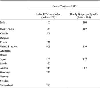
India, data apply to 1913/14. Fuel is from Indian Admin Report (1913/14), pp. 470–71; all other Railroad Statistics of the United States or RUS (1916) p. 143. US: data are applied to 1910. Fuel and employees, Fishlow (1966) p. 613, 620; ton miles, pass miles, revs, miles RUS (1913), pp. 81, 87; RUS (1916), pp. 40, 43. Canada: data apply to 1913. Fuel Green (1986), p. 807; locomotives RUS (1916), p. 48; all other RUS (1913), p. 122. Argentina: data apply to 1913 and are from estadistica ferrocarriles en explotacion (1913). Russia: data apply to 1909. Fuel Coal Tables (BPP 1913 vol. 285), p. 48; all other RUS (1916) p. 140. Brazil: data apply to 1912 and are from RUS (1916), p. 141. Coal is provided by Summerhill and is based on his (2003) book. France: data apply to 1911. Fuel Coal Tables (BPP 1913 vol. 285), p. 48; all other RUS (1916) p. 135. United Kingdom: data apply to 1912. Fuel Coal Tables (BPP 1913 vol. 285), p. 48; employees RUS (1913), p. 123; all other RUS (1916) p. 133. Belgium: data apply to 1911 and for state railways only. Fuel Coal Tables (BPP 1913 vol. 285), p. 48; all other RUS (1916) p. 136. Japan: data apply to 1911/12. Fuel Coal Tables (BPP 1913 vol. 285), p. 48; locomotives and vehicles RUS (1916) p. 142; all other RUS (1913) p. 131. Germany: data apply to 1913 and are from RUS (1916), p. 134. Switzerland: data apply to 1914 and are from RUS (1916), p. 137. Austria: data apply to 1913 and are from RUS (1916), p. 138. Norway: data apply to 1914 and are from RUS (1916), p. 139. Sweden: data apply to 1914 and are from RUS (1916), p. 139. Labor efficiency index is calculated from Clark (1988), table 3, machinery per worker (in loom equivalents). The U.S. figure is for United States (South) only. Output per spindle is also from Clark (1988), table 5.
While labor was not as productive, Indian railways performed better in other dimensions. India had one of the highest output per ton of fuel, even higher than the United States. India's output per track mile was also higher than most countries, ahead of Canada, France, Norway, and Sweden. We can approximate the relative TFP levels of railway systems by calculating a weighted average of the log of the indices for output per worker, output per unit of fuel, and output per track mile.Footnote 21 India's TFP was behind the United States, Canada, Russia, and Belgium, similar to Japan, France, and the United Kingdom, and ahead of Brazil and Argentina.Footnote 22 The relative TFP measures are preliminary because they do not adjust for quality differences in output, capital, labor, and fuel across countries. That said, they provide strong suggestive evidence that Indian railways compared favorably to railways in many countries especially in terms of fuel and track productivity.
Table 4B presents a series on labor efficiency and capital productivity for cotton textiles from Greg Clark (1988). Labor efficiency is measured as machinery per worker (in loom equivalents). In other words, it captures one aspect of capital per worker in the textile sector. India clearly has low labor efficiency by world standards. For example, English workers manned four times more looms than Indian workers, while Austrian and German workers manned 2.5 times more looms than Indian workers.Footnote 23 Unfortunately, we cannot construct the number of employees manning locomotives or engines in railways because the labor data are not disaggregated by task, which would allow for a more precise comparison. But, the aggregate figures on locomotives per worker suggest that capital per worker was relatively low in Indian railways much like it was in cotton textiles. The big difference comes from capital productivity. When output per locomotive or output per vehicle is compared with hourly output per spindle in cotton textiles, Indian railways fare much better. The UK-India comparison is especially striking in this regard. Output per locomotive in the United Kingdom was just a quarter of that in India compared to output per spindle, which was 16 percent higher in the United Kingdom. Thus, Indian railway performance compared favorably to higher income countries and to Indian performance in the cotton textile industry.

RAILWAYS AND THE GROWTH OF THE INDIAN ECONOMY
The growth of railway TFP had implications for the colonial Indian economy. In this section, we quantify the contribution to Indian national income and relate it to social savings estimates. As in the pioneering works of Robert Fogel (1966) and Albert Fishlow (1965), economic historians often measure the developmental impact of railways using the social savings methodology. The social savings are calculated as the freight rate difference between the preexisting technology and railways multiplied by railway output in some benchmark year. As Nicholas Crafts (2004) highlights, a decrease in freight rates is equivalent to an increase in TFP and therefore the social savings can also be calculated using the change in TFP. Crafts’ approach modifies a standard growth accounting equation and decomposes the growth in income per person into terms for the TFP growth and capital per worker growth of different sectors in the economy. If one focuses on the role of TFP growth only, the calculation is straightforward.Footnote 24 The growth contribution of railways is equal to the average annual rate of TFP growth multiplied by the share of railway revenues in national income. We apply this formula using our new estimates of TFP growth.
Before proceeding, it is important to note that our estimates do not capture the full social savings from Indian railways. Railways increased transport productivity in large part by displacing wagons and coaches, or in the case of India, bullock carts. We estimate TFP growth starting in 1874 when most of the trunk lines had been built and so earlier productivity advances associated with displacement of carts are not measured. The same applies to new railways entering our sample. To summarize, our growth contribution attributed to railways only captures the increase in TFP from 1874 to 1912 and the increase in TFP post-railway construction.
Our calculations show that increases in railway TFP were an important engine of growth for the Indian economy. Railway revenues accounted for around 3 percent of Indian national income in 1912.Footnote 25 Following Crafts method, multiplying 0.03 by the average annual TFP growth rate, 2.31, implies that railway TFP growth contributed 0.07 percent per year to Indian GDP per capita. By comparison, Angus Maddison (2003) estimates that Indian GDP per capita grew at 0.6 percent per year from 1870 to 1913. Thus the gains from railway TFP growth are equal to 12 percent of the total GDP per capita growth in the decades leading up to World War I. Compounding the gains in TFP over a 38-year period implies a social savings of 2.7 percent of GDP in 1912.
How do the social savings associated with TFP growth compare with other estimates of social savings? Hurd (1983) estimates that Indian GDP would have been 9 percent lower in 1900 without railways. Dave Donaldson (2012) finds a similar estimate (9.7 percent social savings in 1930) by studying the relationship between Indian railways and agricultural income. The estimated TFP contribution reported here (2.7 percent in 1912) is close to one-third of their estimates for social savings. We regard one-third as a relatively large share given we focus on a more narrow time period from 1874 to 1912. More importantly, the one-third share highlights the importance of TFP growth in explaining the aggregate effect of Indian railways. Had railway productivity remained at its 1874 level, the Indian economy would have been 3 percent smaller in 1912. In short, it mattered a lot how railways were operated in India.
SOURCES OF TFP GROWTH
Railway TFP growth was clearly a major factor in Indian income growth from 1874 to 1912. In this final section, we explore the sources of TFP growth. There have been major advances in the study of productivity over the last 20 years, including TFP growth decomposition and attention to the identification of TFP determinants (see Syverson 2011 for an overview). We draw on this literature to estimate the importance of reallocation effects, capacity utilization, and technological adoption.
Reallocation Effects
It is obvious that industries will become more productive if their firms increase in productivity. Probing deeper though reveals several components. Industries can become more productive simply because the market share of more productive firms increases. Industry-level productivity can also rise if firms entering the market are more productive than the average firm or if exiting firms are less productive than the average. The combination of the last three factors is known in the productivity literature as “reallocation.” The Lucia Foster, John Haltiwanger, and C. J. Krizan (2001) decomposition, or FHK for short, quantifies the contribution of reallocation. It decomposes annual industry-level TFP growth into the following five terms

where θit is the market share for firm i in year t, tfpit is the natural log of TFP for firm i in year t, TFPt is the weighted average productivity across all firms in year t defined by equation 3, e is the set of entering firms in year t, x is the set of exiting firms in year t, and n is the set of incumbent firms in year t. The reallocation effect is defined as the sum of the second and fourth terms minus the fifth term. The second term  captures the effect of increasing or decreasing the market share of more productive firms as measured by Δθit. The fourth term
 captures the effect of entry. Notice that industry productivity rises if entering firms are more productive than the industry average in the previous year. The fifth term
 captures the effect of exit and is subtracted to capture the gains from eliminating unproductive firms. The remaining sources of industry TFP growth are called the “within effect.” The first term
 is often the most important and measures within railway TFP growth holding market share constant.
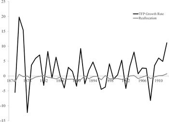
We find that reallocation did not play a key role in Indian railways. Figure 3 plots industry TFP growth (the black line) and the contribution of reallocation (the grey line). TFP growth was volatile from year to year, but little of the variation was due to reallocation. Most industry TFP growth was due to within railway TFP growth holding market share constant. Moreover, the reallocation effect is generally negative lowering TFP growth by an average of 0.5 percent per year.
Reallocation reduced TFP growth in part because entering railways tended to be less productive than incumbents. There were entrants in 15 years of our sample and all were before 1901. In 10 of the 15 years, the TFP of entrants was below the average for incumbent railways. The aggregate effect of entry was not large in the end and reduced industry productivity growth by an average of only 0.08 percent per year. Exiting railways also tended to be less productive than the average railway. Normally the exit of less productive firms raises industry TFP, but in Indian railways the exit effect was muted because exits did not mean the end of services on a line, but simply a merger to a larger system.
ROLE OF REALLOCATION IN TFP GROWTH

The greatest retarding factor in reallocation was the shift in market share away from the most productive lines. The East Indian, for example, was among the most productive railways in every year, but its market share declined from 47 percent in 1874 to 25 percent by 1912. The FHK decomposition shows that the average effect of changes in market share among incumbents was to lower industry TFP growth by an average of 0.5 percent per year. Such patterns are a sign that competition was limited in Indian railways. In competitive markets more productive firms usually gain market share by offering lower prices. For some reason, competition did not work in this manner for Indian railways. Overall the FHK decomposition points to the importance of within-railway TFP growth that we explore below.
Capacity Utilization
In studying the sources of TFP growth for U.S. railroads during the nineteenth century, Fishlow (1966) argued for the importance of capacity utilization. Fishlow explained how utilization is related to building ahead of demand and how it influences the measurement of productivity:
“For capital intensive and capital durable sectors faced with indivisibilities, the size of the capital stock is not a good proxy for the annual flow of services it delivers. At their inception, firms will typically be burdened with higher capital-output ratios than current demand seems to dictate, due both to technical considerations and to positive expectations. Only over time will capital services attain a stable relationship with the magnitude of the stock…. Because the capital stock has been used as an input, part of the measured productivity gains of railroads…derives from this phenomenon of increasing utilization” (p. 630).
Fishlow goes on to argue that capital utilization can explain between one-sixth and one-third of productivity growth in U.S. Railroads between 1840 and 1910. Did capacity utilization play a similar role in India? A good indicator of utilization is the number of train miles run per track mile because it measures usage of the fixed network. Train miles run per track mile is also revealing because railway track is generally constant in quality. Other measures of utilization, like vehicle loads per train, are more conflated with technological change.
In the Indian context, 1876 is the first year where train miles are reported in the official publications. The data show no upward trend until the mid-1890s, but there is a clear increase in track utilization after 1895. From 1895 to 1912 train miles run per track mile increased by more than 40 percent across all the railways in our sample. To quantify the contribution of track utilization to TFP, we modify our Cobb-Douglas production function to include a railway-level measure of track utilization in each year. Our approach is similar to other works that measure economies of density by including utilization terms directly in the cost or production function (Oum, Waters, and Yu 1999).Footnote 26
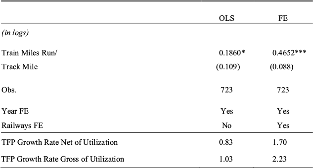
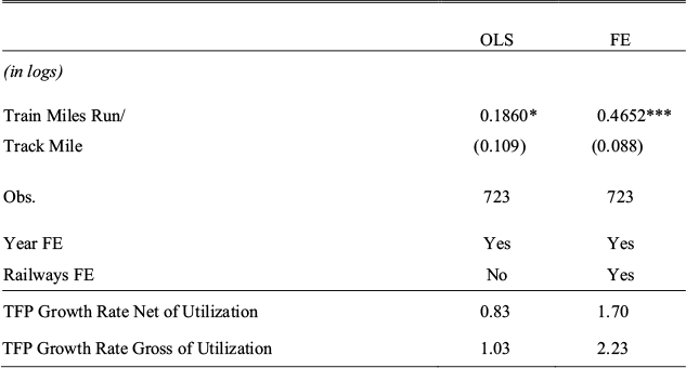
Table 5 reports the coefficients on track utilization. Unsurprisingly, greater track utilization increases output. In the FE model, for example, the elasticity of track utilization is 0.46. Although significant, the coefficient is not large enough to explain all the TFP growth. Track utilization increased by more than 40 percent, but industry-level TFP almost doubled in this period. Calculations of TFP growth net of utilization confirm that capacity utilization is not the major driver of TFP growth. At the bottom of Table 5, we report the rate of net TFP growth from 1876 to 1912.Footnote 27 We also report the average TFP growth rate without accounting for utilization for comparison. Average annual TFP growth rates are lower, but not substantially. Track utilization accounts for 20 to 25 percent of TFP growth in most specifications.
THE CONTRIBUTION OF CAPACITY UTILIZATION TO TFP
* = Significant at the 10 percent level
** = Significant at the 5 percent level
*** = Significant at the 1 percent level
Notes:
Robust standard errors clustered at the railway level in parentheses. Regressions include capital (in rupees), labor and fuel as in Table 2. Data covers years 1876–1912 because information on train miles is unavailable for 1874/75.
Thus, our estimates show that while capacity utilization was important in the Indian context, most of the TFP growth within railway systems was driven by other factors.
Technological and Organizational Change
In most industries, technological and organizational changes are the most important drivers of TFP growth. In the late nineteenth and twentieth century, railway technology improved significantly throughout the world. But, it is unclear whether India participated in this technological advance. The state of technology on Indian railways circa 1900 is summarized in the Robertson Report (1903). The author, Thomas Robertson, argued that Indian railways lagged behind railways in advanced countries like the United States, Canada, and Britain. According to Robertson, Indian railways were using few of the best practice technologies such as automatic vacuum brakes, gas and electrical lighting, high capacity bogie vehicles, and interlocking signal systems for railway stations. But over the 1900s Indian railways increased their adoption of new technologies and their relative backwardness changed by 1912.
In 1890 only 11 percent of engines and 1 percent of vehicles were fitted with vacuum brakes.Footnote 28 By 1912, 81 percent of engines and 47 percent of vehicles were fitted with brakes. Previously one worker had to be present on each engine and vehicle and concurrently pull the brake in order for the train to stop. With such automatic brakes the entire train could be brought to a halt quickly thereby increasing safety. Interlocking signal systems at stations also improved safety. With this technology signals on the track were locked when a train entered the route and were unlocked only after the train had passed. The average number of stations with interlocking systems increased from 17 to 55 percent between 1902 and 1912. A similar change occurred in electrical and gas lighting. In 1900, 40 percent of the rolling stock was lighted by gas. It increased to over 70 percent by 1912. Electrical lighting, superior to gas lighting because it gave off less heat, was largely absent in the early 1900s, but by 1912, 17 percent of the rolling stock was lighted by electricity. Thus, Indian railways were moving closer to the technology frontier by 1912 in adopting what experts considered best-practice technologies.
Similar to other studies of TFP (for example, Rosegrant and Evenson 1992), we assess the correlation between these notable technological changes and our estimates of railway-level TFP.Footnote 29 The technology variables are measured in terms of adoption rates. For example, bogie coaches refer to the proportion of all coaches with the bogie technology. Our main goal is to evaluate the joint significance of the technology variables in explaining the variation in TFP across and within railways over time. We use the F-statistic to test whether all the coefficients on the technology variables are jointly equal to zero. The list of technologies is limited to what was quantified in the official reports and emphasized by Robertson (1903).
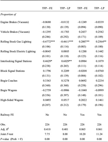
The F-statistics, p-values, and technology coefficients are reported in Table 6 using different railway-level TFP estimates in specifications with and without railway fixed effects. Across the four specifications, we can strongly reject the null that the technology coefficients are jointly equal to zero. Comparing the R-squared in a specification with railway fixed effects to one with railway fixed effects and the technology variables suggests that the technology variables can explain 7.3 percent of the variation in TFP within railways over the 1900s. In terms of individual technologies, we find positive effects for gas lighting of the rolling stock. Most other variables have a positive sign but are not statistically significant. The imprecision may be related to correlations in the adoption of different technologies.
More broadly the results in Table 6 suggest that technological change explains some of the TFP growth in Indian railways. Several other examples, like innovations in locomotive power, support this view.Footnote 30 However, not all technologies worked to improve productivity. Railways gauges are the most controversial technological choice in Indian railways. Similar to other countries, the Indian network was not built on a uniform gauge. Lines were constructed on the standard, meter, and narrow gauge. Gauge diversity can be a source of inefficiency because traffic has to be unloaded and reloaded at breaks of gauge. Unfortunately, we cannot estimate the direct impact of breaks of gauge because we do not have detailed information on traffic flows between railway systems. That said, we find evidence of TFP growth in all systems regardless of gauge. The meter gauge system appears to have lower levels of TFP compared to the standard gauge but the trend in TFP between 1874 and 1912 is similar to the standard gauge.
Finally, Indian railways experienced a shift to colonial government ownership over our period of analysis. As described in section 2, the initial network was constructed by privately owned British companies backed by a government guarantee. Beginning in 1879 the government began to take over the private companies although many of them were allowed to retain operations. Based on the historical experiences of other countries, one might expect government takeovers to reduce productivity (Shleifer 1998; Bogart 2010). However, in other work, we find this transition to government ownership decreased operating costs, particularly labor costs (Bogart and Chaudhary 2012a). Qualitative evidence also suggests the colonial government may have raised labor productivity. It introduced a profit sharing agreement with state railway employees in 1880. The Railway Provident Fund contributed a portion of state railway earnings, disbursing them to employees in proportion to their salary and position. In the 1900s many government railways also began providing schools for the children of railway employees or reimbursing fees at neighboring public schools. Such measures suggest railway authorities may have been paying efficiency wages to their employees although the subsidy appears to be small.Footnote 31
THE RELATIONSHIP BETWEEN TECHNOLOGY ADOPTION AND TFP

* = Significant at the 10 percent level.
** = Significant at the 5 percent level.
*** = Significant at the 1 percent level.
Notes:
Data only covers years 1900 to 1912. Robust standard errors clustered at the railway level in parentheses. *** p < 0.01, ** p < 0.05, * p < 0.1. The technology variables are measured in terms of adoption rates. For example, bogie coaches capture the proportion of coaches with the bogie technology.
Finally, the Government of India also organized “railway conferences,” to create exchanges between state railway officials and companies. The first railway conference in 1880 introduced a code of general rules for the working of all lines, including agreements for the interchange of rolling stock, a uniform classification of goods, and accounting standards. Subsequent conferences in the 1880s and 1890s tried to assimilate the construction of rolling stock. A special committee met regularly to adopt standards, arrange experiments, and publish research (Bell 1894, p. 114).
The actions of the colonial government towards the railway sector may be surprising in light of a broader critique that it failed to contribute to development. We think the explanation is based in fiscal incentives. Gross railway revenues as a proportion of total government revenues increased from less than 5 percent in the 1870s to just over 30 percent by 1912 (Bogart and Chaudhary 2012b). The government stood to gain substantial revenues by improving or at least maintaining railway TFP.
CONCLUSION
Using new data on individual railways, we find strong evidence of TFP growth in Indian railways from 1874 to 1912. Our estimates suggest that TFP growth averaged 2.3 percent per year. TFP growth had a large aggregate impact on the Indian economy adding 0.07 percent per year to Indian income per capita, and generating a social savings of 2.7 percent between 1874 and 1912.
The performance of Indian railways stands in sharp contrast to the limited productivity growth in agriculture and cotton textiles, another key modern industrial sector of this period. Indian railways also compared favorably to railways in advanced economies such as Britain and the United States, especially in terms of fuel and capital productivity. Although scholars may be right that railways could have done more to generate economic growth in India before World War I, it is hard to criticize the sector based on its productivity performance.
We find there is not any single factor, which was the main driver of TFP growth. Technological changes made important contributions, as did greater capacity utilization and organization changes. However, reallocation within the industry played no role and in fact negatively influenced productivity. In concluding, we note that the success of Indian railways did not last. A number of performance indicators, like ton-miles per worker and real freight charges, stagnate or reverse from 1920 to Indian Independence in 1947 (Hurd 2007, Bogart and Chaudhary 2012b). Thus Indian railways acted as “engines of growth” only during the first era of globalization. Explaining why the productivity growth of Indian railways stopped around 1920 is a key issue for future research.