





Introduction
Current swine production systems emphasize maximal growth performance through nutrient oversupply. This practice results in significant nutrient excretion via feces and urine, contributing to environmental pollution – an issue that has gained increasing global concern (McKee and Bradley et al. Reference McKee, Bradley and Shelley2021). Feed expenditures comprise approximately 60–70% of total production expenses in swine operations (Patience and Rossoni-serão et al. Reference Patience, Rossoni-Serão and and Gutiérrez2015), where energy and protein ingredients emerge as the major formulation cost factors (Noblet and Wu et al. Reference Noblet, Wu and and Choct2022). To optimize livestock production sustainability, producers should employ mathematical modeling to quantify the relationship between nutrient provision and swine growth performance. This enables data-driven feed formulation adjustments that minimize nutrient excretion while maintaining productivity, thereby enhancing both economic efficiency and environmental stewardship in the production systems (Wang et al. Reference Wang, Hu and Wang2022a). Two widely recognized reference standards exist for energy requirements in growing-finishing pigs: the National Research Council (NRC, 2012) guidelines and the Chinese Feeding Standard of Swine (GB/T 29235-2020). Both standards derive from comprehensive syntheses of empirical research findings. Given advancements in breeding technologies and husbandry practices over the past few decades, it is unclear whether these standards accurately reflect current porcine energy requirements.
Meta-analysis represents a statistical approach for research synthesis that quantitatively aggregates results from numerous independent studies examining related hypotheses, thereby increasing statistical power and enabling robust conclusions (Catalá-lópez et al. Reference Catalá-lópez, Alonso-arroyo and Hutton2014). Its characteristics include increasing the sample size to enhance the credibility of conclusions, minimizing subjective influence and maximizing the scientific and authenticity of the findings (Hernandez et al. Reference Hernandez, Marti and Roman2020). While initial meta-analytic efforts in animal science were largely confined to genetic investigations (Li et al. Reference Li, Wan and Lin2023), contemporary approaches have increasingly employed this methodology to examine nutritional interventions, production parameters and feeding strategies (Zheng et al. Reference Zheng, An and Du2024). For example, meta-analysis was used to determine the ratio of tryptophan to lysine in piglets (Simongiovanni et al. Reference Simongiovanni, Corrent and Le Floc’h2012), and to identify the individual and interactive effects of different factors on the performance and feed efficiency of finishing pigs (Douglas et al. Reference Douglas, Szyszka and Stoddart2015). The meta-analysis was also used to evaluate the impact of polyunsaturated fatty acids on pork quality and growth performance (Wang et al. Reference Wang, Huang and Wang2021). However, current literature reveals a paucity of meta-analytic investigations specifically addressing energy-dependent feed intake regulation in finishing swine. Therefore, essential opportunities exist to employ meta-analysis for comprehensive evaluation of nutrient-growth performance interactions in modern pig production systems.
To our knowledge, limited studies have used meta-analysis to predict energy intake in finishing pigs and then verified the impact of this prediction on their growth performance with a specific pig feeding trial (Hou et al. Reference Hou, Wang and Wen2022). Therefore, based on existing research, this study employs the statistical method of meta-analysis to construct mathematical models of the relationship between body weight (BW) and daily intake of digestible energy (DE) in growing-finishing pigs. The optimal model was selected to predict the nutritional requirements of growing-finishing pigs. Precision feeding regimens based on this model were evaluated to assess the effects of feeding strategies that regulate energy intake on the growth performance, serum biochemistry, antioxidant indicators and gut microbiota structure of finishing pigs.
Materials and methods
Data sources for meta-analysis
The data were sourced from journal articles published between 2002 and 2024 (Supplementary Table 1). Considering the advancements in pig breeding that have led to changes in genetic backgrounds, data from earlier literature were not included. In English databases such as Web of Science, PubMed and Google Scholar, the search terms used were “(pig OR swine) AND growth performance.” In Chinese databases, including China National Knowledge Infrastructure, Wanfang Data and VIP Database, the search terms were “pig” and “growth performance.” Based on the titles and abstracts, a preliminary screening was conducted of the literature that met the inclusion criteria, resulting in 1075 articles. For the obtained literature, the following criteria were applied for selection: 1) The study was conducted in China, involving pig breeds such as Duroc, Landrace, Large White or their crossbreeds, with research content related to the growth performance and dietary energy and protein intake of growing-finishing pigs; 2) each study had ≥3 treatment levels with ≥3 repetitions per treatment, excluding studies where individual pigs were the experimental units, as this design lacks true independent replicates for statistical analysis of treatment effects at the experimental unit level; 3) the study provided complete dietary formulations and growth performance data; 4) the study employed a completely randomized block design, with an equal number of male and female pigs in each treatment, allowing animals to feed freely, with a minimum experimental period of 14 days.
Datasets preparation
The first author, number of treatments, initial and final weights and growth performance data extracted from the selected papers were recorded in a template. The parameters included the average daily gain (ADG), average daily feed intake (ADFI), feed-to-gain ratio (F/G), dietary DE, dietary crude protein (CP) percentage, average daily intake of DE and average daily intake of CP for pigs under each treatment diet. If any of the above parameters were missing, they were calculated based on other reported parameters in the paper (if available); otherwise, the entire record was discarded (Wang et al. Reference Wang, Hu and Wang2022a). The average BW of pigs fed each feed treatment was calculated by averaging the initial and final weights of all pigs in the same treatment group. The first authors were sorted, and different treatment groups by the same author were assigned the same number, ranging from 1 to 112, designated as “No.”
Model selection and fitting
Theoretically, even when using the same database, the predicted results from different functional models can vary significantly (Cai et al. Reference Cai, Cai and Tang2024). Therefore, it is necessary to establish multiple functional models to achieve a more appropriate fit. This study evaluates three alternative models to describe and predict the relationship between daily energy intake and average BW: The linear mixed-effects (LME), Bayesian ridge regression (BRR) and random forest regression (RFR) models.
The primary distinction between fixed and random effects in an LME model is that fixed effects are considered unknown parameters, whereas random effects are regarded as random variables drawn from a distribution, such as a normal distribution (Yu et al. Reference Yu, Guindani and Grieco2022). Import the compiled meta-analysis dataset into RStudio software. The model formula, taking the quadratic polynomial random slope model as an example, is as follows:
 \begin{equation*}\text{DE} = {{\beta}_{\text{0}}}\text{+}{{\beta}_{\text{1}}}\cdot poly{{(BW,2)}_1}+{{\beta}_{\text{2}}}\cdot poly{{(BW,2)}_2}+uNo.+\epsilon\end{equation*}
where DE is digestible energy, poly (BW, 2)1 and poly(BW, 2)2 are quadratic polynomial terms for BW, representing linear and quadratic effects of BW, respectively. β 0 is the intercept, and β 1 and β 2 are fixed-effects coefficients for linear and quadratic effects, respectively. uNo. is inter-study heterogeneity (that is, a random effect) and represents the random contribution of different study groups (No.) to the model. ϵ is the residual (error term).
In mixed-effects models, the core role of random effects is to capture the differences between groups (experiments) and the calculation of random effects is based on the group number (No.), which does not affect the outcome of the model regardless of the order of the group numbers (Moyer et al. Reference Moyer, Heagerty and Murray2022).
BRR is a machine learning algorithm used to solve regression problems, particularly suitable for datasets with high-dimensional features (Fisher and Mehta Reference Fisher and Mehta2015). In this study, the Bayesian ridge linear model is employed to investigate the relationship between the dependent variable DE and the independent variable BW, accounting for the non-independence of observations across groups identified by No. The model is implemented using the stan_glmer function from the rstanarm package in R (version 4.4.1). The model formula is as follows:
 \begin{equation*}{\text{DE}_{ij}} = {{\beta}_{\text{0}}}\text{+}{{\beta}_{\text{1}}}\cdot B{W_{ij}}+{b_{No.i}}+{\epsilon_{ij}}\end{equation*}
where DEij represents the digestible energy of the j individual in the i experimental group, BWij represents the corresponding BW, β 0 and β 1 are the intercept and slope of the fixed effect, bNo.i is the random intercept for the i is the experimental group and ϵij is the error term. In the Bayesian framework, the model parameters are given a semi-student t distribution as a prior. Markov chain Monte Carlo method was used to fit the model. Four chains were set; each chain had 2000 iterations; the random seed was 123; and the adaptive sampling parameter adapt_delta = 0.95. The median was used as the predicted value in this study.
The Random Forest algorithm, developed by Breiman, has its greatest advantage in its ability to uncover meaningful interactions and nonlinear effects among predictor variables (Rigatti Reference Rigatti2017). The dataset was partitioned into a training set and a test set, with 70% of the data allocated to the training set and 30% to the test set. In this study, a random forest model was employed to predict the dependent variable DE, utilizing all available predictor variables in the dataset. The model was implemented using the ranger function from the ranger package in R (4.4.1). The model was configured to construct 500 decision trees. During each split in the decision trees, the algorithm considers a random subset of two predictor variables.
Fattening pig and diet
This research was specifically approved by the Animal Care and Use Committee of Zhejiang University (Ethics Code Permit ZJU20250392). This experiment was conducted in the year 2025, and 16 healthy “Duroc × Landrace × Large White” crossbred castrated male pigs were used as the experimental subjects, with an average initial BW about 85 kg. During the experimental period, each pig was housed individually and all experimental pigs had free access to water daily. The experimental feed consisted of granulated feed for the finishing period, with the composition and nutritional levels of the basal diet presented in Table 1. The basal diet was formulated to meet or exceed the nutrient requirements of finishing pigs as recommended by the Chinese national standard GB/T 39235-2020 (Nutrient Requirements of Pigs).
Basic diet composition and nutritional level

Table 1 Long description
Ingredients are listed with content in percent, alongside nutrient levels with their content values. Ingredient contents are maize grain 31 percent, barley 36 percent, soybean meal 9 percent, wheat bran 10 percent, wheat flour 10 percent, and premix marked with b 4 percent, with total 100 percent. Nutrient levels marked with a list DE 13.67 MJ per kg and ME 13.25 MJ per kg. Additional nutrient contents are CP 13.0 percent, CF 4.5 percent, Ca 0.65 percent, and TP 0.50 percent. Total amino acids listed are Lys 0.90 percent and Met 0.25 percent.
a Crude protein was calculated values, while the other nutrient levels were measured values based on the “Chinese Feed Composition and Nutritional Value Table (33rd edition, 2022).” Lys and Met are presented as total amino acids.
b Premix provided the following per kg of diets: VA 7500 IU; VD3 1350 IU; VE 25 IU; VK3 1.8 mg; VB1 1.2 mg; VB2 3.6 mg; VB6 3.0 mg; VB12.20 μg; Nicotinic acid 25 mg; Pantothenic acid 15 mg; Folic acid 1.1 mg; Biotin 0.425 mg; Choline chloride 100 mg; NaCl 2.4 g; Fe 130 mg; Mn 42 mg; Zn 100 mg; Cu 24.8 mg; I 0.4 mg; Se 0.3 mg.
Grouping and feeding of pigs
Sixteen pigs were randomly assigned to two groups: The control (Con) group and the meta-analysis (Meta) group, with eight pigs in each group. Each pig was individually housed and served as a statistical unit (n = 8). The Con group was allowed ad libitum feeding, with daily feed intake measured. The Meta group received the restricted feed calculated based on calculations from a meta-analysis function. The pigs in the Meta group were weighed every three days to obtain BW data for analyzing weight changes during the experimental period. The feed intake for the Meta group was adjusted based on a fitted BW–energy intake model derived from the meta-analysis training. The model was used to calculate daily energy intake, which was then used to determine the daily feed allowance based on the DE level of the diet provided in Table 1. The daily feed allowance was calculated as follows:
Daily feed allowance = Daily energy intake/Digestible energy level of the diet.
Feeding was conducted twice daily at 09:00 and 15:00, with each feeding session providing half of the day’s feed allowance. The experimental period lasted for 42 days, during which feed intake, BW and backfat changes were recorded for both groups.
Sample collection
Backfat thickness was measured using a B-mode ultrasound scanner (Xinyu Muke Technology Co., Ltd.) at the P2 position, defined as 6.5 cm lateral to the dorsal midline at the level of the last (13th) rib. This measurement was used to analyze changes in backfat thickness. On the day before the end of the experiment, blood was collected from each pig via the anterior jugular vein. The blood samples were centrifuged at 3000 g at 4℃ for 10 minutes to separate the serum, which was then stored at −20℃ for subsequent serum biochemical analysis. Fresh fecal samples were also collected for the determination of apparent digestibility of total organic carbon (TOC). Following the experiment, pigs from both groups were subjected to slaughter. Contents of the colon were retrieved for the analysis of gut microbiota structure using 16S rRNA gene amplicon sequencing.
Analysis of serum biochemical, antioxidant indexes and apparent digestibility of TOC
Serum glucose (GLU), triglyceride (TG), total cholesterol, total protein, low-density lipoprotein cholesterol (LDL-C), high-density lipoprotein cholesterol, alkaline phosphatase, alanine aminotransferase (ALT), aspartate aminotransferase (AST), creatine kinase, urea, lactate dehydrogenase (LDH), total antioxidant capacity and malondialdehyde were detected by kits (Nanjing Jiancheng Bioengineering Institute).
Determination of the Hydrochloric acid-insoluble ash concentration in feed and feces followed the method described by the regulations and requirements of Determination of Hydrochloric acid-insoluble ash in feed (China, GB/T 23742-2009, General Administration for Quality Supervision, Inspection and Quarantine of China, 2009).
TOC was measured following the method of Walkley and Black (Walkley and Black Reference Walkley and Black1934). The apparent metabolic rates were determined by the endogenous indicator method (Wang et al. Reference Wang, Liu and Zhao2022b). The determination of CP content was carried out in accordance with the method recorded in GB/T 6432-2018.
16S rRNA library construction and sequencing of content sample
DNA was extracted from fecal samples using a DNA extraction kit (QIAGEN, Germany). The quality of the total DNA was assessed using a Thermo NanoDrop 2000 spectrophotometer (ThermoFisher, USA) and 1% agarose gel electrophoresis. The V3-V4 region of the bacterial 16S rRNA gene was amplified using universal primers 341F (5′-CCTAYGGGRBGCASCAG-3′) and 806R (5′-GGACTACNNGGGTATCTAAT-3′). PCR products were analyzed using 2% agarose gel electrophoresis and subsequently purified using the AxyPrep DNA Gel Extraction Kit (AxyGEN Company). The amplicons were converted to sequencing libraries using the Illumina TruSeq DNA PCR-Free Library Preparation Kit (Illumina, USA). The libraries were sequenced on the MiSeq/HiSeq platform (Illumina, Inc., San Diego, CA, USA) to generate paired-end 500/250 bp reads. Demultiplexed FASTQ files were generated from the raw data using bcl2fast (v2.20.0.422). ASV sequences and tables were obtained using the previous method (Tang et al. Reference Tang, Liu and Ma2021). The α and β diversities were assessed using R software (version 4.4.1) based on the ASV table, and the microbial community structure was analyzed at the genus level.
Data analysis
All experimental data were analyzed using independent samples t-tests with GraphPad Prism (9.1). Data are presented as mean ± standard error of the mean. The statistical tests included unpaired two-tailed Student's t-test. A P-value of less than 0.05 was considered to indicate a significant difference, while a P-value between 0.05 and 0.1 was considered to indicate a significant trend.
Results
Database in the meta-analysis
Based on the literature screening criteria, a total of 523 treatments from 112 articles were included in this study (Fig. 1). The collected data encompassed the genetic background of each group of pigs during the study trials, average intake of DE and CP, initial and final BWs along with their averages and growth performance indicators (ADG, ADFI, F/G and body length [BL]). A comprehensive database for meta-analysis was established (Aymerich et al. Reference Aymerich, Tokach and Dritz2021) (Supplementary Table 1). The descriptive statistics of the overall meta-analysis database in Table 2.
Literature retrieval and screening process of the meta-analysis.

Figure 1 Long description
The flowchart outlines the process of identifying studies through databases and registers. It begins with the identification phase, where related articles are identified through database searching, totaling 1075 articles. The screening phase follows, with 601 articles screened. During this phase, experiments are removed if growth performance and dietary energy and protein intake data are not from China, accounting for 474 removals. Articles sought for retrieval number 435, with 166 removed due to having three or fewer treatment gradients and replicates. Articles assessed for eligibility total 307, with 128 removed for lacking complete dietary formulation with data on growth performance. The final inclusion phase results in 112 articles with 523 selections processed and used for the meta-analysis. Any point not conforming is excluded, including those not following a completely randomized design, having half male and half female pigs, eating freely and lasting at least 14 days, resulting in 195 exclusions.
Descriptive statistics of the database of the meta-analysis
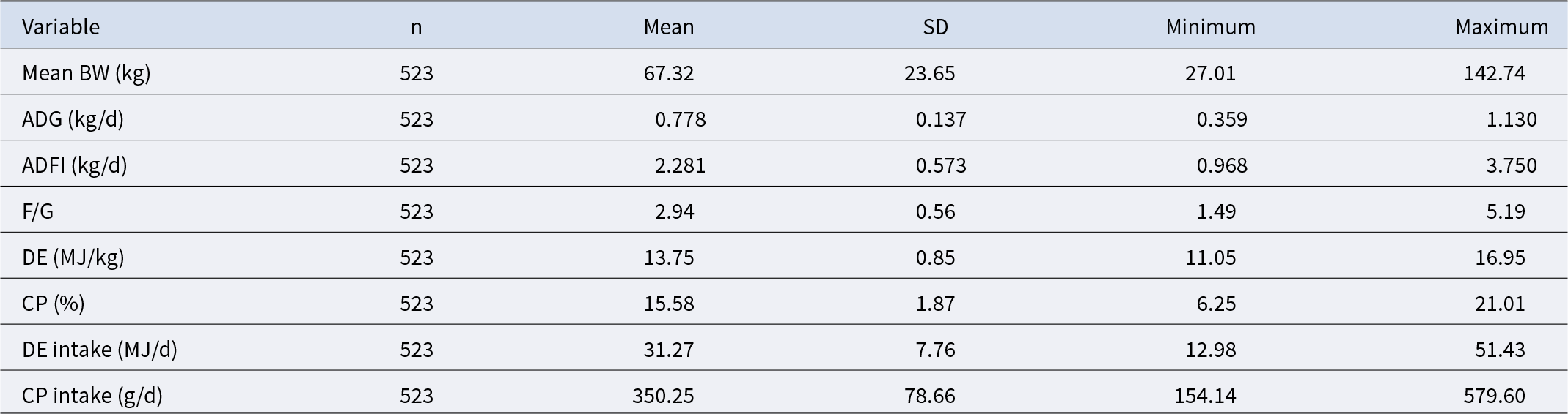
Table 2 Long description
Descriptive statistics are reported for eight variables, each with n 523, including Mean BW, ADG, ADFI, F/G, DE, CP, DE intake, and CP intake. ADG has a mean of 0.778 kg per day with SD 0.137, minimum 0.359 and maximum 1.130. ADFI has a mean of 2.281 kg per day with SD 0.573, minimum 0.968 and maximum 3.750. F/G has a mean of 2.94 with SD 0.56, minimum 1.49 and maximum 5.19. DE is 13.75 MJ per kg on average with SD 0.85, minimum 11.05 and maximum 16.95, and CP averages 15.58 percent with SD 1.87, minimum 6.25 and maximum 21.01. DE intake averages 31.27 MJ per day with SD 7.76, minimum 12.98 and maximum 51.43, and CP intake averages 350.25 g per day with SD 78.66, minimum 154.14 and maximum 579.60.
Establishment of models
Through the preliminary fitting curve, we discovered that the relationship between DE and BW is nonlinear, and changes in BW significantly affect DE intake, which implies some laws (Fig. 2A). We then used LME, BRR and RFR models to establish the relationship between BW and DE of growing-finishing pigs. In the LME model, the red line in the fitting graph indicates that the model simulates the relationship between DE and BW well. In this model, the quadratic polynomial random slope model had a relatively larger R 2 (coefficient of determination), while the Akaike information criterion and Bayesian information criterion were smaller (Fig. 2B). The parameters of the model are shown in Table 3. Then, the residual and Q-Q plots well evaluate the performance of the LME model (Fig. 3A). Within the BRR framework, the parameters are shown in Table 4. The analysis of the residual and Q–Q plots indicates that the model demonstrates a satisfactory level of reliability (Fig. 3B). The RFR model yielded a mean squared error of 7.95 for the relationship between DE and BW with a coefficient of determination (R 2) of 0.86, surpassing the benchmark of 0.80 and the residual and Q–Q plots of the RFR model signifying a robust model fit (Fig. 3C). Ideally, all data points in the scatter plot should be on the red line, with the predicted values of the RFR model also clustered around the red line (Fig. 3D). This observation shows that the prediction of the model is relatively close to the actual value, indicating that the prediction accuracy is high.
Preliminary observation of DE and BW relationships and visualization of LME fitting models. (A) Scatter plots and fitted curves for DE and BW. (B) Visualization of DE and BW relationships in LME models. The fixed-effects fit curves are shown in blue; the complete fit curve is shown in red.
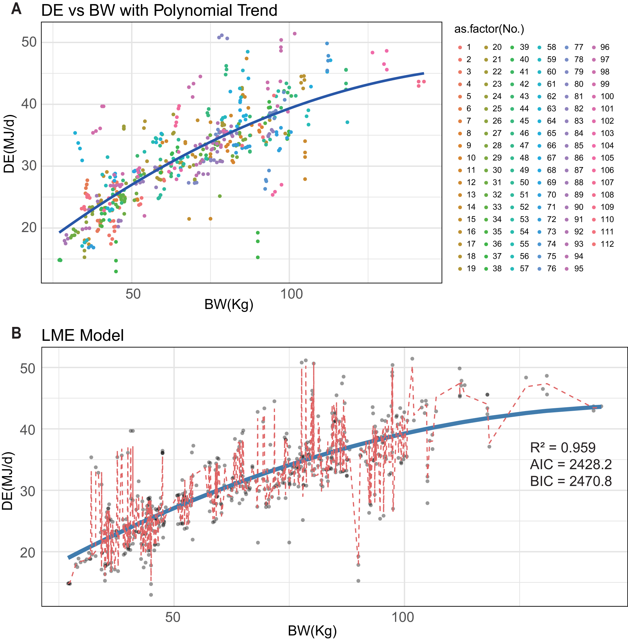
Figure 2 Long description
A scatter plot titled ′DE vs BW with Polynomial Trend.′ The horizontal axis is labeled BW in kilograms, ranging from 0 to 150. The vertical axis is labeled DE in megajoules per day, ranging from 10 to 50. Various colored data points are scattered across the plot, with a blue polynomial trend line running through them, indicating a nonlinear relationship between DE and BW. A legend on the right lists numbers associated with different colors, ranging from 1 to 112. The image B shows a scatter plot titled ′LME Model.′ The horizontal axis is labeled BW in kilograms, ranging from 0 to 150. The vertical axis is labeled DE in megajoules per day, ranging from 10 to 50. Grey data points are scattered across the plot, with a blue line representing the LME model fit. Red dashed lines connect some of the data points, indicating variability. The plot includes statistical values: R squared equals 0.959, Akaike Information Criterion equals 2428.2 and Bayesian Information Criterion equals 2470.8.
The fitting effect of each model. (A) Residuals and Q–Q plots for DE and BW of LME model. (B) Residuals and Q-Q plots for DE and BW of BRR model. (C) Residuals and Q–Q plots for DE and BW of RFR model. (D) A comparison between the actual DE and the values predicted by the RFR model.

Figure 3 Long description
Two plots titled, Residuals for LME Model and, Normal Q minus Q Plot. The Residuals for LME Model plot has the horizontal axis labeled, Fitted values, with tick labels 0, 200, 400 and the vertical axis labeled, Residuals, with tick labels negative 5, 0, 5. A scatter of points spans fitted values from 0 to about 500 and residuals from about negative 7 to about 7. A horizontal reference line is drawn at residual equals 0. The point cloud is densest around residual 0, with several points above 5 and below negative 5. The Normal Q minus Q Plot has the horizontal axis labeled, Theoretical Quantiles, with tick labels negative 3, negative 1, 1, 3 and the vertical axis labeled, Sample Quantiles, with tick labels negative 5, 0, 5. Points follow the reference line near the middle and curve away at the ends, with the lowest points below negative 5 and the highest points above 5. The image B showing two plots titled, Residuals for BRR Model and, Normal Q minus Q Plot. The Residuals for BRR Model plot has the horizontal axis labeled, Fitted values, with tick labels 200, 300, 400, 500 and the vertical axis labeled, Residuals, with tick labels negative 200, negative 100, 0, 100. A scatter of points spans fitted values from about 180 to about 520 and residuals from about negative 220 to about 140. A horizontal reference line is drawn at residual equals 0. Most points cluster around residual 0, with a low outlier near residual about negative 200. The Normal Q minus Q Plot has the horizontal axis labeled, Theoretical Quantiles, with tick labels negative 3, negative 1, 1, 2, 3 and the vertical axis labeled, Sample Quantiles, with tick labels negative 200, negative 100, 0, 100. Points follow the reference line near the middle and diverge at the ends, including a low point near sample quantiles about negative 200 and high points above 100. The image C showing two plots titled, Residuals for RFR Model and, Normal Q minus Q Plot. The Residuals for RFR Model plot has the horizontal axis labeled, Fitted values, with tick labels 0, 100, 200, 300 and the vertical axis labeled, Residuals, with tick labels negative 15, negative 5, 5, 15. A scatter of points spans fitted values from 0 to about 350 and residuals from about negative 17 to about 18. A horizontal reference line is drawn at residual equals 0. The densest band of points is around residual 0, with several points near negative 15 and near 15. The Normal Q minus Q Plot has the horizontal axis labeled, Theoretical Quantiles, with tick labels negative 3, negative 1, 1, 2, 3 and the vertical axis labeled, Sample Quantiles, with tick labels negative 15, negative 5, 5, 15. Points track the reference line near the center and curve away at both ends, reaching below negative 15 and above 15. The image D showing one scatter plot titled, Actual vs Predicted. The horizontal axis is labeled, Actual DE, with tick labels 20, 30, 40, 50. The vertical axis is labeled, Predicted DE, with tick labels 20, 30, 40, 50. Points form an upward slanting cluster from about actual 18 and predicted 18 to about actual 50 and predicted 50. A straight diagonal reference line is drawn from the lower left toward the upper right. Many points lie close to the diagonal line, with some points above and below it across the range. Across A, B and C, the residual plots show point clouds centered around the residual equals 0 reference line, with different vertical spreads: about negative 7 to 7 in A, about negative 220 to 140 in B and about negative 17 to 18 in C. The normal Q minus Q plots in A, B and C show points close to the reference line in the middle and larger departures at the lowest and highest quantiles, with the largest labeled sample quantile range shown in B from about negative 200 to above 100.
Parameters of LME models
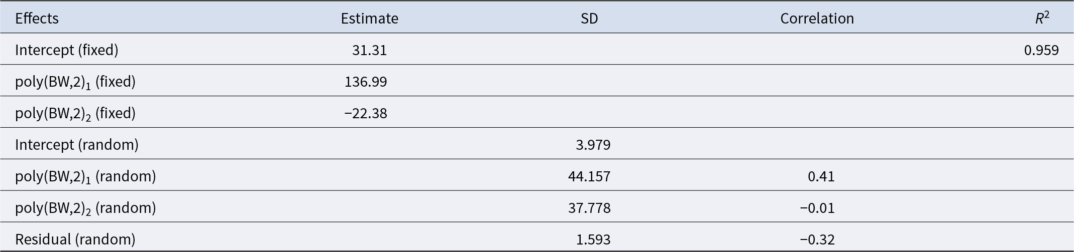
Table 3 Long description
Columns are Fixed Effects, Estimate, SD, Correlation, and R2. Fixed effects list an intercept with estimate 31.31 and R2 0.959, plus poly BW degree 2 term 1 with estimate 136.99 and poly BW degree 2 term 2 with estimate minus 22.38. Random effects list an intercept with SD 3.979. Random poly BW degree 2 term 1 has SD 44.157 with correlation 0.41. Random poly BW degree 2 term 2 has SD 37.778 with correlation minus 0.01. Residual random effect has SD 1.593 with correlation minus 0.32.
Parameters of the BRR models
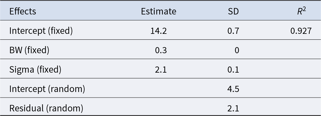
Table 4 Long description
Effects are listed with columns for Estimate, SD, and R2. For fixed effects, Intercept has an estimate of 14.2, SD 0.7, and R2 0.927. BW has an estimate of 0.3 and SD 0, with no R2 shown. Sigma has an estimate of 2.1 and SD 0.1, with no R2 shown. For random effects, Intercept has no estimate shown and SD 4.5, with no R2 shown. Residual has no estimate shown and SD 2.1, with no R2 shown.
The nutrient intake generated by the model was compared with the data provided by the NRC (2012) and the GB/T 29235-2020, as shown in Table 5. It can be observed that for DE intake, the LME model’s estimate for energy intake was closer to the values from the NRC (2012) and the GB/T 29235-2020. At the same time, the R2 value of the LME model is 0.959, which is higher than that of the BRR model (0.927) and the RFR model (0.86). Thus, we determined that the LME model was the most suitable model, and then conducted subsequent analysis.
Comparison of models-generated DE intake to those presented in NRC (2012) and GB/T 29235-2020
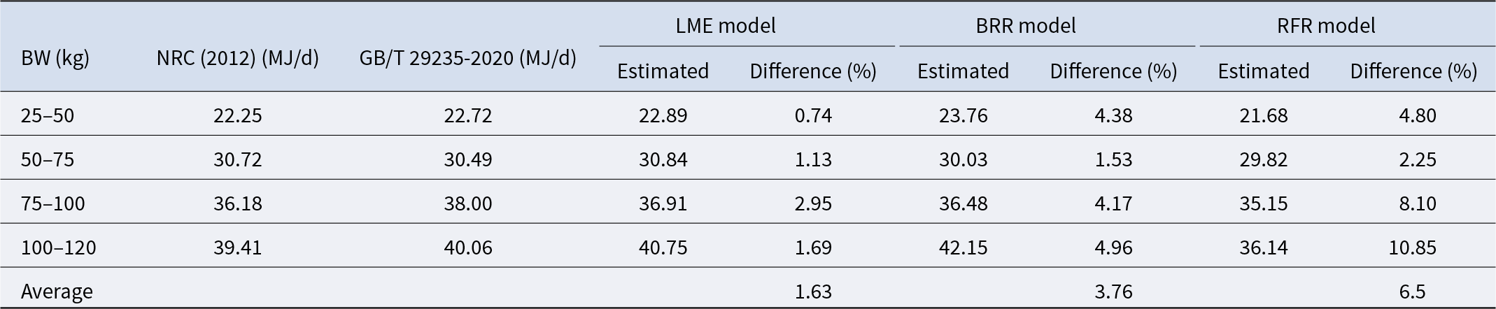
Table 5 Long description
Digestible energy intake is listed in megajoules per day for four body weight ranges, with reference values from NRC 2012 and GB/T 29235 to 2020, plus estimated values and percent differences for LME, BRR, and RFR models. For 25 to 50 kilograms, NRC is 22.25 and GB/T is 22.72; LME estimates 22.89 with 0.74 percent difference, BRR estimates 23.76 with 4.38 percent difference, and RFR estimates 21.68 with 4.80 percent difference. For 50 to 75 kilograms, NRC is 30.72 and GB/T is 30.49; LME is 30.84 with 1.13 percent difference, BRR is 30.03 with 1.53 percent difference, and RFR is 29.82 with 2.25 percent difference. For 75 to 100 kilograms, NRC is 36.18 and GB/T is 38.00; LME is 36.91 with 2.95 percent difference, BRR is 36.48 with 4.17 percent difference, and RFR is 35.15 with 8.10 percent difference. For 100 to 120 kilograms, NRC is 39.41 and GB/T is 40.06; LME is 40.75 with 1.69 percent difference, BRR is 42.15 with 4.96 percent difference, and RFR is 36.14 with 10.85 percent difference. An Average row lists percent differences only: 1.63 for LME, 3.76 for BRR, and 6.5 for RFR.
Note: Difference (%) means models predict compared to GB/T 29235-2020.
Effects of precision feeding on finishing pigs
Performance
As shown in Table 6, no significant difference was observed between the initial and final weight of finishing pigs in either group. Following a 42-day feeding trial, a significant reduction in the F/G was observed in the Meta group as compared to the Con group (P < 0.05). Additionally, the ADFI in the Meta group demonstrated a highly significant decrease, with a P-value less than 0.0001. ADG, backfat gain and BL also did not show significant changes.
Effects of feeding methods calculated by meta-analysis on growth performance of finishing pigs
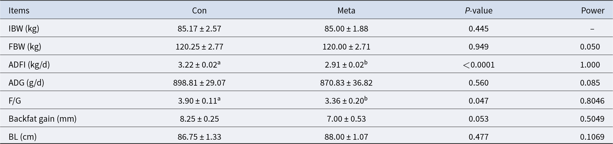
Table 6 Long description
Growth performance items are listed for Con and Meta, with columns for P-value and Power. IBW in kilograms is 85.17 plus or minus 2.57 for Con and 85.00 plus or minus 1.88 for Meta, with P-value 0.445 and Power shown as a dash. FBW in kilograms is 120.25 plus or minus 2.77 for Con and 120.00 plus or minus 2.71 for Meta, with P-value 0.949 and Power 0.050. ADG in grams per day is 898.81 plus or minus 29.07 for Con and 870.83 plus or minus 36.82 for Meta, with P-value 0.560 and Power 0.085. F over G is 3.90 plus or minus 0.11a for Con and 3.36 plus or minus 0.20b for Meta, with P-value 0.047 and Power 0.8046. Back fat gain in millimeters is 8.25 plus or minus 0.25 for Con and 7.00 plus or minus 0.53 for Meta, with P-value 0.053 and Power 0.5049. BL in centimeters is 86.75 plus or minus 1.33 for Con and 88.00 plus or minus 1.07 for Meta, with P-value 0.477 and Power 0.1069.
Note: In the same row, values with no letter or the same letter superscripts mean no significant difference (P > 0.05), while different small-letter superscripts mean a significant difference (P < 0.05).
Antioxidant capacity, serum biochemical parameters, apparent digestibility of TOC and fecal sample CP content
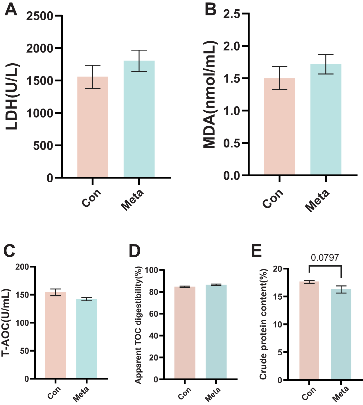
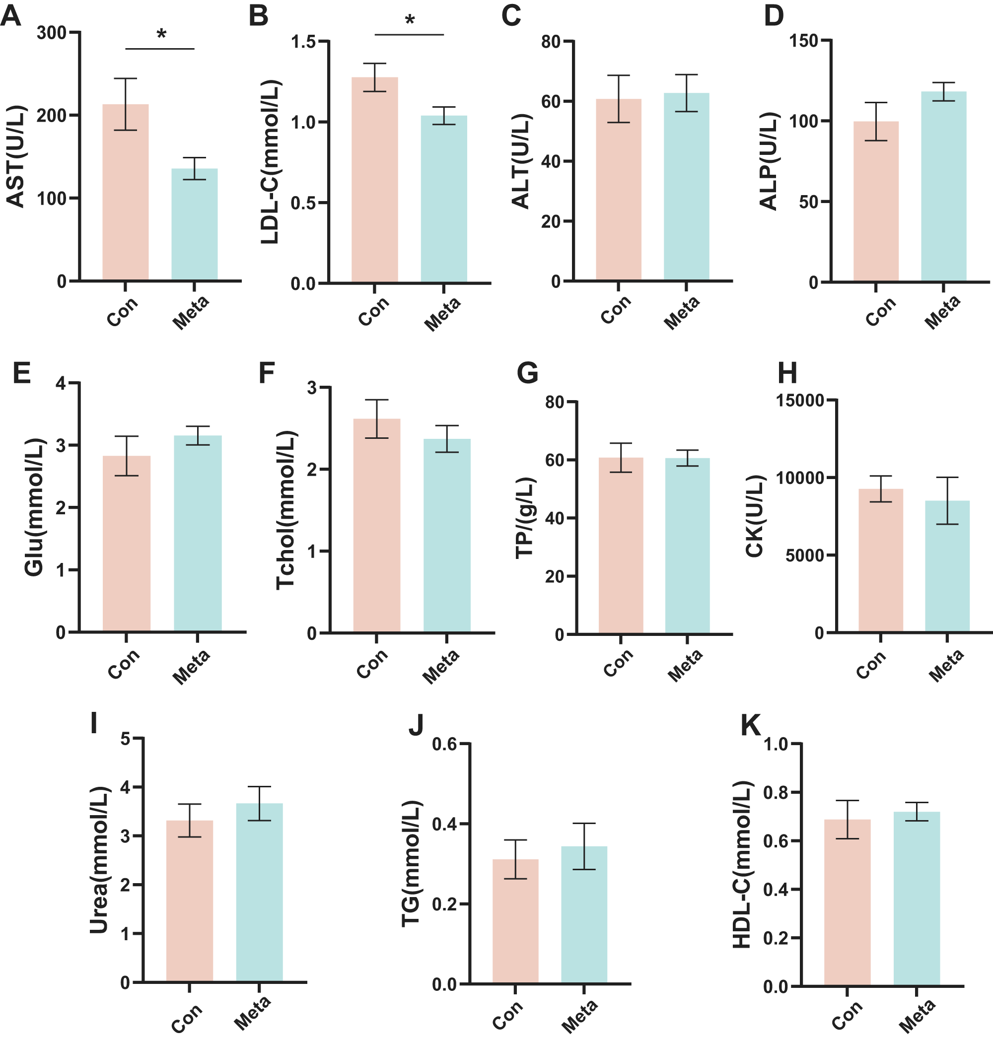
There were no significant differences in serum LDH, malondialdehyde and total antioxidant capacity between the two groups at the end of the experiment (Fig. 4A–C). The meta-analytical evaluation of various feeding regimens revealed an average apparent digestibility rate of TOC of 84.73 ± 0.74% for the Con group and 86.45 ± 0.87% for the Meta group (Fig. 4D). The CP content of the fecal samples in the Meta group showed a downward trend (P = 0.0797, Fig. 4E). The serum levels of AST and LDL-C of fattening pigs in Meta group were significantly lower than those in Con group (P < 0.05, Fig. 5A, B), and there were no significant differences in other indicators (Fig. 5C–K).
Effects on antioxidant capacity, apparent digestibility of total organic carbon and fecal sample crude protein content in finishing pigs. (A) Level of LDH. (B) Level of MDA. (C) Level of T-AOC in two groups of growing-finishing pigs. (D) Level of apparent digestibility of total organic carbon. (E) Level of fecal sample crude protein content. Statistical analysis: unpaired two-tailed Student’s t-test for the comparison of two groups (n = 8, ****P < 0.0001; *P < 0.05).

Figure 4 Long description
A bar graph with the x-axis labeled, Con and Meta and the y-axis labeled, LDH with unit U over L. The y-axis ranges from 0 to 2500. The Con bar is at about 1550. The Meta bar is at about 1800. Both bars have vertical error bars. The image B showing a bar graph with the x-axis labeled, Con and Meta and the y-axis labeled, MDA with unit nanomol over mL. The y-axis ranges from 0.0 to 2.5. The Con bar is at about 1.5. The Meta bar is at about 1.7. Both bars have vertical error bars. The image C showing a bar graph with the x-axis labeled, Con and Meta and the y-axis labeled, T-AOC with unit U over mL. The y-axis ranges from 0 to 200. The Con bar is at about 155. The Meta bar is at about 140. Both bars have vertical error bars. The image D showing a bar graph with the x-axis labeled, Con and Meta and the y-axis labeled, Apparent TOC digestibility with unit percent. The y-axis ranges from 0 to 100. The Con bar is at about 85. The Meta bar is at about 87. Both bars have vertical error bars. The image E showing a bar graph with the x-axis labeled, Con and Meta and the y-axis labeled, Crude protein content with unit percent. The y-axis ranges from 0 to 20. The Con bar is at about 17.5. The Meta bar is at about 16.5. Both bars have vertical error bars. A bracket spans the two bars with the text, 0.0797, above the bracket.
Effects on serum biochemical parameters in finishing pigs. (A) Level of AST. (B) Level of LDL-C. (C) Level of ALT. (D) Level of ALP. (E) Level of Glu. (F) Level of Tcho. (G) Level of TP. (H) Level of CK. (I) Level of Urea. (J) Level of TG. (K) Level of HDL-C in the serum of growing-finishing pigs. Statistical analysis: unpaired two-tailed Student’s t-test for the comparison of two groups (n = 8, ****P < 0.0001; *P < 0.05).

Figure 5 Long description
A bar chart with x axis labels, Con and Meta and y axis label, AST open parenthesis U over L close parenthesis, ranging from 0 to 300. The Con bar is about 210 and the Meta bar is about 135. A horizontal bracket with an asterisk is shown above the two bars. The image B showing a bar chart with x axis labels, Con and Meta and y axis label, LDL dash C open parenthesis millimole over L close parenthesis, ranging from 0.0 to 1.5. The Con bar is about 1.3 and the Meta bar is about 1.05. A horizontal bracket with an asterisk is shown above the two bars. The image C showing a bar chart with x axis labels, Con and Meta and y axis label, ALT open parenthesis U over L close parenthesis, ranging from 0 to 80. The Con bar is about 60 and the Meta bar is about 62. The image D showing a bar chart with x axis labels, Con and Meta and y axis label, ALP open parenthesis U over L close parenthesis, ranging from 0 to 150. The Con bar is about 100 and the Meta bar is about 120. The image E showing a bar chart with x axis labels, Con and Meta and y axis label, Glu open parenthesis millimole over L close parenthesis, ranging from 0 to 4. The Con bar is about 2.8 and the Meta bar is about 3.2. The image F showing a bar chart with x axis labels, Con and Meta and y axis label, Tchol open parenthesis millimole over L close parenthesis, ranging from 0 to 3. The Con bar is about 2.6 and the Meta bar is about 2.4. The image G showing a bar chart with x axis labels, Con and Meta and y axis label, TP open parenthesis gram over L close parenthesis, ranging from 0 to 80. The Con bar is about 61 and the Meta bar is about 60. The image H showing a bar chart with x axis labels, Con and Meta and y axis label, CK open parenthesis U over L close parenthesis, ranging from 0 to 15000. The Con bar is about 9500 and the Meta bar is about 8500. The image I showing a bar chart with x axis labels, Con and Meta and y axis label, Urea open parenthesis millimole over L close parenthesis, ranging from 0 to 5. The Con bar is about 3.3 and the Meta bar is about 3.7. The image J showing a bar chart with x axis labels, Con and Meta and y axis label, TG open parenthesis millimole over L close parenthesis, ranging from 0.0 to 0.6. The Con bar is about 0.32 and the Meta bar is about 0.35. The image K showing a bar chart with x axis labels, Con and Meta and y axis label, HDL dash C open parenthesis millimole over L close parenthesis, ranging from 0.0 to 1.0. The Con bar is about 0.70 and the Meta bar is about 0.72.
Gut microbiota from fecal sample
The Venn diagrams showed that the Con and Meta groups have different amplicon sequence variants (ASVs) with 2686 and 2685 unique ASVs, respectively (Fig. 6A). A total of 1039 shared ASVs were identified, comprising 16.2% of the overall ASV pool. Alpha diversity assessment was subsequently conducted. In comparison with the control group, the Meta group displayed reduced Shannon, Richness, Simpson and Chao1 indexes, although these differences did not reach statistical significance (Fig. 6B–E). The principal coordinate analysis, based on the weighted UniFrac distance of ASVs, indicated significant alterations in the structural composition of the gut microbiome for the Meta group (Fig. 6F). To evaluate meta-analysis-derived feeding method impacts on gut microbiota, the relative abundance analysis and difference analysis of microbes at the genus level were carried out (Fig. 6G). When contrasted with the Con group, the Meta group exhibited a marked decrease in the relative abundance of Clostridium_sensu_stricto_1, Lachnospira and Sarcina (P < 0.05, Fig. 6H), whereas a significant increase was noted in the relative abundance of Bacteroidales_RF16_group, Clostridium_sensu_stricto_6, Colidextribacter, Olsenella and Peptococcus (P < 0.05, Fig. 6I).
The feeding method based on meta-analysis changed the intestinal microbes in finishing pigs. (A) Venn diagram of intestinal ASV number in finishing pigs. (B–F) Difference analysis of α, β diversity index of intestinal microbiota in finishing pigs. (G) Composition of intestinal microbiota of finishing pigs at genus level. (H) Bacteria with a relatively decreased abundance at the genus level. (I) Bacteria with a relatively increased abundance at the genus level. Statistical analysis: unpaired two-tailed Student’s t-test for the comparison of two groups (n = 8; **P < 0.01; *P < 0.05).

Figure 6 Long description
A Venn diagram with two circles labeled, Con and Meta. The Con-only section shows 2686 and 41.9 percent. The overlap shows 1039 and 16.2 percent. The Meta-only section shows 2685 and 41.9 percent. The image B showing a bar chart with the vertical axis labeled, Shannon, ranging from 0 to 6. Two bars are labeled, Con and Meta. A bracket above the bars shows, P equals 0.64. The Con and Meta bars are at similar heights, near 5. The image C showing a plot with the vertical axis labeled, Richness, ranging from 700 to 1000. Two groups are labeled, Con and Meta. A bracket above the groups shows, P equals 0.86. Both groups show a central marker near the mid 800s with vertical spread; the Con group includes a point near 650 and the Meta group includes a point near 700. The image D showing a box plot with the vertical axis labeled, Simpson, ranging from 0.93 to 0.99. Two groups are labeled, Con and Meta. Text shows, P equals 0.29. The Con box is centered higher than the Meta box, with Con values clustered around about 0.97 to 0.98 and Meta values clustered around about 0.95 to 0.97. The image E showing a violin plot with the vertical axis labeled, Chao1, ranging from 400 to 1200. Two groups are labeled, Con and Meta. Text shows, P equals 0.86. The Con distribution spans a wider range and extends higher than the Meta distribution; both groups have central markers around the 800 to 900 range. The image F showing a scatter plot with the horizontal axis labeled, PCo1, 8.872 percent, ranging from negative 0.4 to 0.2 and the vertical axis labeled, PCo2, 8.219 percent, ranging from negative 0.2 to 0.4. A legend labeled, group, lists Con and Meta. Points are labeled C1 through C8 and M1 through M8. Two outlined ellipses surround the Con points and the Meta points. The Con points cluster mainly at positive PCo1 values around 0.0 to 0.2, with one point near PCo2 about 0.35. The Meta points cluster mainly at negative PCo1 values around negative 0.35 to negative 0.1, with PCo2 values around 0.0. The image G showing a stacked bar chart titled, Comparison of Genus Abundance. The vertical axis is labeled, Average Abundance, ranging from 0.00 to 1.00. Two stacked bars are labeled, Con and Meta. A legend titled, Genus, lists ChristensenellaceaeR-7group, Clostridiumsensustricto1, Clostridiumsensustricto1, Escherichia-Shigella, LachnospiraceaeNK4A136group, Lactobacillus, Muribaculaceae, others, Prevotella, RF39, Romboutsia, Streptococcus, Treponema, UCG-002 and UCG-005. The Con and Meta stacked bars show similar overall composition, with multiple segments of varying heights. The image H showing three bar charts with overlaid points and the vertical axis labeled, log2 Relative Abundance plus 1, ranging from 0.000 to 0.125. The three titles are Clostridiumsensustricto1, Lachnospira and Sarcina. Each chart compares Con and Meta. A legend labeled, groupID, lists Con and Meta. In Clostridiumsensustricto1, the Con bar is higher than the Meta bar, with a bracket marked asterisk. In Lachnospira, the Con bar is higher than the Meta bar, with a bracket marked asterisk. In Sarcina, the Con bar is higher than the Meta bar, with a bracket marked two asterisks. The image I showing five bar charts with overlaid points and the vertical axis labeled, log2 Relative Abundance plus 1, ranging from 0.000 to 0.006. The five titles are BacteroidalesRF16group, Clostridiumsensustricto6, Colidextribacter, Olsenella and Peptococcus. Each chart compares Con and Meta. A legend labeled, groupID, lists Con and Meta. In BacteroidalesRF16group, the Meta bar is higher than the Con bar, with a bracket marked asterisk. In Clostridiumsensustricto6, the Meta bar is higher than the Con bar, with a bracket marked asterisk. In Colidextribacter, the Meta bar is higher than the Con bar, with a bracket marked asterisk. In Olsenella, the Meta bar is higher than the Con bar, with a bracket marked asterisk. In Peptococcus, the Meta bar is higher than the Con bar, with a bracket marked two asterisks. Across the set of graphs, Con and Meta are compared for overlap counts in the Venn diagram, multiple diversity metrics with P values shown, separation of labeled points in the PCo plot, overall genus composition in stacked bars and genus-specific differences in the small multiple bar charts.
Discussion
Providing precise dietary energy and nutrients formulations is crucial for maximizing growth performance and minimizing the environmental impact of swine production (Zhang and Adeola Reference Zhang and Adeola2017). BW of pigs reflects their current physiological condition and is a key factor affecting their energy requirements and the efficiency of nutrient digestion and absorption (Nyachoti and Zijlstra et al. Reference Nyachoti, Zijlstra and de Lange2004). Although studies have shown that net energy can better predict pig growth performance (Noblet and Van Milgen Reference Noblet and Van Milgen2004), DE is more readily available in practice and has widespread adaptability in global applications (Morgan et al. Reference Morgan, Cole and Lewis1975). Therefore, this study, based on meta-analysis, used pig BW as the independent variable and energy intake as the dependent variable to establish LME, BRR and RFR models. The results show that the LME model is the best in terms of visualization; in comparison with GB/T 29235-2020, the difference (%) in each stage is the smallest of the three models. At the same time, it also has the highest R 2 value among the three models. Therefore, we finally chose the LME model for the experiment.
In this study, the precision feeding of growing-finishing pigs based on the LME model effectively resulted in a form of restricted feeding. The restricted feeding involves providing animals with fewer nutrients than they would consume ad libitum, with the aim of reducing excessive fat deposition and enhancing feed efficiency (Chen et al. Reference Chen, Chen and Lin2020). A previous study found that restricted feeding has a greater impact on growth performance and subsequent compensatory growth than protein restriction (Weremko et al. Reference Weremko, Skiba and Raj2013). Calorie restriction may affect metabolism, reduce obesity and improve intestinal microbiota (Liu et al. Reference Liu, Wei and Di2024). Our study showed that the ADFI of finishing pigs was lower than that of the ad libitum group, while growth performance and backfat thickness were similar between the two groups, and the F/G ratio significantly decreased. This result indicates that the feeding method based on energy intake calculated from meta-analysis can improve feed efficiency and reduce feeding costs without significantly compromising the growth performance of finishing pigs. At the same time, although our difference index has a validity of over 0.8, more samples will be used in the future to verify this formula at different time points.
AST and ALT, the two most active transaminases in the body, play an important role in amino acid metabolism (Marín-garcía and Llobat et al. Reference Marín-garcía, Llobat and López-Lujan2022). When animals are stressed or experience organ damage, AST leaks out of the cells into the bloodstream, resulting in increased serum AST enzyme activity (Liu et al. Reference Liu, Ji and Zhang2015). A previous study has demonstrated that serum AST levels are closely related to liver fat accumulation caused by obesity and associated metabolic syndromes (Vega et al. Reference Vega, Adams-huet and Peshock2006). LDL-C is a cholesterol-rich lipoprotein that transports cholesterol to peripheral tissue cells, with a relatively high content potentially inducing diseases. In this study, the observed reductions in AST and LDL-C suggest that precision feeding not only supports normal protein and cholesterol metabolism in finishing pigs but also enhances liver health, thereby curbing excessive fat deposition and associated metabolic disorders.
The gut microbiota plays a vital role in host health. Bacteroidales may function by regulating the host’s carbohydrate metabolism and reducing insulin resistance (Niu et al. Reference Niu, Zhao and Xiang2022). Colidextribacter can produce short-chain fatty acids such as butyrate and has been identified as a potential probiotic due to its positive effects in certain diseases, including obesity-related metabolic disorders (Yang et al. Reference Yang, Li and Wen2021). Olsenella is associated with obesity and metabolic dysfunction in mice and humans, as well as gut inflammation and serum TGs (Guadagnini et al. Reference Guadagnini, Rocha and Santos2019). Peptococcus has been shown to be involved in the prevention of viral cancers (Ubachs et al. Reference Ubachs, Ziemons and Soons2021). Interestingly, in our study, the majority of the microbial groups with significantly increased abundance are beneficial to the host’s health, while the decline in the abundance of certain bacterial communities has an adverse effect on the host’s health. For example, Clostridium_sensu_stricto_1 is positively correlated with gut inflammation and the high expression of pro-inflammatory cytokines that disrupt gut barrier integrity, and its reduced abundance can alleviate gut inflammation to some extent (Abdelbary et al. Reference Abdelbary, Hatting and Bott2022). Sarcina, while not pathogenic, is associated with gastric ulcers and delayed gastric emptying, which can lead to perforation (Sopha et al. Reference Sopha, Manejwala and Boutros2015). The microbial abundance variation suggested that the precision feeding used in this study has a positive effect on maintaining normal lipid and fiber metabolism in finishing pigs, protecting gut barrier integrity and alleviating gastrointestinal inflammation. However, the present model was validated using data from finishing pigs with BWs ranging from 85 to 120 kg. Accordingly, its application within this weight range is supported. For pigs weighing <85 kg or >120 kg, predictive accuracy has not been evaluated. Users should exercise caution when extrapolating beyond this range, and future studies should validate the model using independent data from lighter or heavier pigs. This meta-analysis did not explicitly account for genetic background or heterosis effects due to inconsistent reporting in primary studies. Future studies with detailed genetic information are needed to refine the estimation of nutritional requirements for purebred versus crossbred pigs.
Conclusion
This study utilized meta-analysis to fit LME, BRR and RFR models for the energy intake requirements of growing-finishing pigs. The LME model demonstrated a better fit. The precise feeding derived from the LME model, compared to ad libitum feeding, can improve feed efficiency and reduce feeding costs without affecting the growth performance of the pigs. Additionally, it lowers serum LDL-C and AST indicators, improving the structure of gut microbiota to some extent, indicating a positive effect on the gut health of pigs. These findings indicate that the model accurately predicts the nutritional requirements of finishing pigs and has potential efficiency applications in optimizing feed formulations for economic improvements and reducing environmental pollution in the pig industry.
Supplementary Material
The supplementary material for this article can be found at https://doi.org/10.1017/anr.2026.10063.
Data Availability Statement
All sequencing data have been uploaded to the SRA under BioProject PRJNA1290262. Metadata for this study can be viewed on the SRA Run Selector at http://www.ncbi.nlm.nih.gov/bioproject/1290262. The model fitting data and code have been uploaded to GitHub at https://github.com/junhai2001l-oss/fitting-models/tree/master. Any other data you may want can be obtained from the author under reasonable circumstances.
Acknowledgements
We would thank Mr. Jianbing Lai for helping in the animal feeding trial.
Author Contributions
H.W. and W.T. conceived and designed the study and method. J.L. and W.T. performed the trial and drafted the manuscript; H.D., J.M. and J.L. analyzed the data; H.W. and Y.M. revised the manuscript. All authors have read and agreed to the published version of the manuscript.
Financial Support
This study was supported by the Key R&D Projects of Zhejiang Province (2022C02015); the National Natural Science Foundation of China (32502916). Project funded by the China Postdoctoral Science Foundation (2024M762857). We acknowledge the financial support from the Selected Funding for Postdoctoral Research Projects of Zhejiang Province (ZJ2024056).
Conflicts of Interest
The authors report no conflicts of interest.




 Open access

