





1 Introduction
This paper is part of our ongoing study of the birepresentation theory of extended affine type
$A_{n-1}$
 Soergel bimodules in characteristic zero, which we started in [Reference Mackaay, Miemietz and VazMMV]. The monoidal category of these Soergel bimodules, denoted
$\widehat {\mathscr {S}}^{\mathrm {ext}}_n$
 in this paper, was studied both algebraically and diagrammatically in [Reference Mackaay and ThielMaTh] and [Reference EliasEli2], and categorifies the extended affine type A Hecke algebra
$\widehat {H}^{\mathrm {ext}}_{n}$
 . This algebra is infinite-dimensional, which on the categorical level corresponds to the fact that
$\widehat {\mathscr {S}}^{\mathrm {ext}}_n$
 is not finitary but wide finitary, in the terminology of [Reference MacphersonMacph]. Whereas finitary birepresentation theory of finitary monoidal categories/bicategories, such as Soergel bimodules of finite Coxeter type, is fairly well developed, see e.g. [Reference Mackaay, Mazorchuk, Miemietz, Tubbenhauer and ZhangMMMTZ1] and [Reference Mackaay, Mazorchuk, Miemietz, Tubbenhauer and ZhangMMMTZ2] and references therein, birepresentation theory of wide finitary monoidal categories/bicategories is still in its infancy. Some fundamental results in finitary birepresentation theory were generalised to the wide finitary setting by Macpherson in [Reference MacphersonMacph], but his framework does not cover triangulated birepresentations, which play a prominent role in the birepresentation theory of
$\widehat {\mathscr {S}}^{\mathrm {ext}}_n$
 . For example, the evaluation birepresentations of
$\widehat {\mathscr {S}}^{\mathrm {ext}}_n$
 in [Reference Mackaay, Miemietz and VazMMV] are triangulated. In this paper, we continue our study of the birepresentation theory of
$\widehat {\mathscr {S}}^{\mathrm {ext}}_n$
 , taking a first step towards the categorification of parabolic induction. As the reader will see, this also involves triangulated birepresentations.
Parabolic induction and restriction play an important role in the finite-dimensional representation theory of
$\widehat {H}^{\mathrm {ext}}_{n}$
 . In particular, for any integers
$1\leq k< n$
 , there is a well-known embedding of algebras

which is the analog of the embedding of finite symmetric groups
$\mathfrak {S}_k\times \mathfrak {S}_{n-k}\to \mathfrak {S}_{n}$
 . Given two finite-dimensional representations
$M_1$
 and
$M_2$
 of
$\widehat {H}^{\mathrm {ext}}_{k}$
 and
$\widehat {H}^{\mathrm {ext}}_{n-k}$
 , respectively, one can use
$\psi _{k,n-k}$
 to define their Zelevinsky tensor product

which is a finite-dimensional
$\widehat {H}^{\mathrm {ext}}_{n}$
 -representation. Zelevinsky [Reference ZelevinskyZel] classified the finite-dimensional irreducible representations of the extended affine type A Hecke algebra in terms of combinatorial objects called multisegments. Leclerc, Nazarov and Thibon [Reference Leclerc, Nazarov and ThibonLNT] gave a necessary and sufficient condition for irreducibility of
$M_1\odot M_2$
 , based on the multisegments corresponding to two finite-dimensional irreducible representations
$M_1$
 and
$M_2$
 .
Now, let
$k_1,k_2,k_3\in \mathbb {Z}_{\geq 1}$
 such that
$k_1+k_2+k_3=n$
 (assuming that
$n\geq 3$
 , of course). Then one can show that

which implies that there is a canonical isomorphism

with
$M_i$
 being a finite-dimensional representation of
$\widehat {H}^{\mathrm {ext}}_{k_i}$
 for
$i=1,2,3$
 . If we define the embedding of algebras

as either one of the two composite maps in (3), then
$M_1\odot M_2 \odot M_3$
 can also be defined directly as

which by the above is canonically isomorphic to either one of the two isomorphic representations in (4).
More generally, let
$k_1, \ldots , k_m\in \mathbb {Z}_{\geq 1}$
 such that
$1\leq m\leq n$
 and
$k_1+\ldots +k_m=n$
 . Then there is an embedding of algebras

which can be used to define the corresponding Zelevinsky tensor product

with
$M_i$
 being a finite-dimensional representation of
$\widehat {H}^{\mathrm {ext}}_{k_i}$
 for
$i=1,\ldots , m$
 , and this tensor product is associative up to canonical isomorphism. For more information on the Zelevinsky tensor product and its role in representation theory, see [Reference Leclerc, Nazarov and ThibonLNT] and references therein.
In this paper, we initiate the categorification of the Zelevinsky tensor product. Specifically, we define a linear, monoidal functor

which categorifies the embedding
$\psi _{k,n-k}$
 in (1). Here
$K^b(\widehat {\mathscr {S}}^{\mathrm {ext}}_n)$
 denotes the homotopy category of bounded complexes in
$\widehat {\mathscr {S}}^{\mathrm {ext}}_n$
 . Before continuing, we should note that
$\psi _{k,n-k}$
 is usually defined in terms of the Bernstein presentation of the extended affine type A Hecke algebra. Unfortunately, there is currently no categorification of
$\widehat {H}^{\mathrm {ext}}_{n}$
 based on that presentation. The decategorification of
$\widehat {\mathscr {S}}^{\mathrm {ext}}_n$
 is naturally associated to the Kazhdan–Lusztig presentation of
$\widehat {H}^{\mathrm {ext}}_{n}$
 , so we define
$\psi _{k,n-k}$
 in terms of that presentation and use it as the starting point for the definition of
$\Psi _{k,n-k}$
 in this paper. Note that in [Reference Stroppel and WedrichStWe], the authors use the categorification of parabolic induction for finite type A Soergel bimodules, where the analog of
$\Psi _{k,n-k}$
 is much easier to define and does not involve Rouquier complexes.
The way to categorify the Zelevinsky tensor product using
$\Psi _{k,n-k}$
 is a bit roundabout, because we do not know how to make sense of something like

where
$\mathbf {M}_1$
 and
$\mathbf {M}_2$
 are finitary birepresentations of
$\widehat {\mathscr {S}}^{\mathrm {ext}}_k$
 and
$\widehat {\mathscr {S}}^{\mathrm {ext}}_{n-k}$
 , respectively. This would require an analog of the balanced box tensor product for module categories over finite tensor categories, defined in [Reference Davydov and NikshychDaNi, Section 2.7], which does not (yet) exist in our setting. Therefore, we follow a different approach, explained below. We first sketch the general idea and then point out some technical hurdles. Recall that, for a fiat bicategory
$\mathcal {C}$
 (e.g. a linear additive pivotal category satisfying certain finiteness conditions), there is a correspondence between transitive finitary birepresentations of
$\mathcal {C}$
 and algebra
$1$
 -morphisms in (the abelianisation of)
$\mathcal {C}$
 , see [Reference Mackaay, Mazorchuk, Miemietz and TubbenhauerMMMT, Corollary 4.8]. Note that in that same paper, and subsequent ones like [Reference Mackaay, Mazorchuk, Miemietz, Tubbenhauer and ZhangMMMTZ2], the correspondence was first formulated with coalgebra
$1$
 -morphisms, instead of algebra
$1$
 -morphisms. For technical reasons, we prefer algebra
$1$
 -morphisms in this paper, see the comments below. Moreover, the bicategories in this paper have only one object and are hence monoidal categories, thus we speak about algebra objects. Any monoidal functor
$\mathcal {C}\to \mathcal {D}$
 between monoidal categories maps algebra objects to algebra objects and can, therefore, be used to induce birepresentations of
$\mathcal {C}$
 to birepresentations of
$\mathcal {D}$
 , which is how we would like to go about categorifying the Zelevinsky tensor product. Unfortunately,
$\widehat {\mathscr {S}}^{\mathrm {ext}}_n$
 is not finitary but wide finitary, and
$\Psi _{k,n-k}$
 does not take values in
$\widehat {\mathscr {S}}^{\mathrm {ext}}_n$
 but in
$K^b(\widehat {\mathscr {S}}^{\mathrm {ext}}_n)$
 .
In [Reference MacphersonMacph], a correspondence between wide finitary birepresentations and (co)algebra objects in some completion is given, but there is currently no analog for triangulated birepresentations. In the examples of finitary or triangulated birepresentations of
$\widehat {\mathscr {S}}^{\mathrm {ext}}_n$
 that we fully understand, the algebra objects are typically given by countable coproducts of tensor products of Soergel bimodules and Rouquier complexes. Hence we introduce certain cocompletions of additive and triangulated monoidal categories/bicategories containing these kinds of algebra objects/1-morphisms in Section 5.2, which are smaller than the completions considered in [Reference MacphersonMacph]. To explain our preference for algebra objects over coalgebra objects in this paper, note that algebra objects typically belong to cocompletions whereas coalgebra objects typically belong to completions. As can be seen from our calculations in Section 5.3, cocompletions are easier to work with in practice. In Section 5.3 we work out the explicit example of the categorified Zelevinsky tensor product
$\mathbf {W}:=\mathbf {V}\boxdot \mathbf {V}$
 of the trivial finitary birepresentation
$\mathbf {V}$
 of
$\widehat {\mathscr {S}}^{\mathrm {ext}}_1$
 with itself. Its construction is technically quite involved. We first define and analyse a wide finitary
$\widehat {\mathscr {S}}^{\mathrm {ext}}_2$
 -birepresentation
$\mathbf {U}$
 corresponding to the algebra object
$\mathrm {Y}:=\Psi _{1,1}(\mathrm {X}\boxtimes \mathrm {X})$
 in the cocompletion of
$K^b(\widehat {\mathscr {S}}^{\mathrm {ext}}_2)$
 , where
$\mathrm {X}$
 is the algebra object in the cocompletion of
$\widehat {\mathscr {S}}^{\mathrm {ext}}_1$
 corresponding to
$\mathbf {V}$
 . Following the terminology introduced in [Reference Mackaay, Miemietz and VazMMV], we call
$\mathbf {U}$
 a wide finitary cover of
$\mathbf {W}$
 . To obtain a triangulated birepresentation, we then observe that
$\mathrm {Y}$
 induces a right action of
$\mathbb {Z}^2$
 on
$K^b(\widehat {\mathscr {S}}^{\mathrm {ext}}_2)$
 which commutes with the left action of
$\widehat {\mathscr {S}}^{\mathrm {ext}}_2$
 , so the orbit category
$\Omega $
 inherits the structure of a
$\widehat {\mathscr {S}}^{\mathrm {ext}}_2$
 birepresentation. We prove that
$\mathbf {U}$
 is equivalent to the full subcategory of
$\Omega $
 whose objects can be identified with those of
$\widehat {\mathscr {S}}^{\mathrm {ext}}_2$
 under the usual embedding into
$K^b(\widehat {\mathscr {S}}^{\mathrm {ext}}_2)$
 . In general, the orbit category of a triangulated category under a group action does not inherit a natural triangulated structure, but in this case we can relate it (via a technical detour which we will explain in Section 5.3.2) to a triangulated orbit category using a dg-enhancement as in [Reference Fan, Keller and QiuFKQ, Theorem/Definition 1.1]. By construction, this triangulated orbit category is a
$\widehat {\mathscr {S}}^{\mathrm {ext}}_2$
 birepresentation and we conjecture that its triangulated Grothendieck group is isomorphic to W, see Conjecture 5.29. It seems likely that this approach can be generalised, but we do not develop a general theory of these kinds of birepresentations and the corresponding algebra objects/1-morphisms in this paper, leaving that for future work.
Something else beyond the scope of this paper is the generalisation of
$\Psi _{k,n-k}$
 to a linear monoidal functor

for
$k_1, \ldots , k_m\in \mathbb {Z}_{\geq 1}$
 such that
$1\leq m\leq n$
 and
$k_1+\ldots +k_m=n$
 , categorifying (5). Conceptually it is clear how to define such a generalisation, but we postpone the lengthy technical details to a future paper. Finally, to prove the categorical analog of (3), i.e., the existence of a natural isomorphism

for
$1\leq k_1, k_2, k_3\leq n$
 such that
$k_1+k_2+k_3=n$
 , we would first need to extend
$\Psi _{k,n-k}$
 to a monoidal functor (with the same notation)

Proving the existence of such an extension is a non-trivial problem and is related to similar extension problems in other contexts, see [Reference Abram, Lamberto-Egan, Lauda and RoseALELR, Conjecture 1.2], [Reference EliasEli2, Section 1.6], [Reference Elias and HogancampElHo] and [Reference Mackaay, Miemietz and VazMMV, Section 1]. The solution of this problem is also a topic for future research.
2 Parabolic embedding: decategorified story
Throughout the paper, let
$n\in \mathbb {Z}_{\geq 1}$
 . For
$n=1$
 , the affine Weyl group
$\widehat {\mathfrak {S}}_1$
 of type
$\widehat {A}_0$
 is the trivial group. Similarly, the finite Weyl group
$\mathfrak {S}_1$
 of type
$A_0$
 is the trivial group.
For
$n\geq 2$
 , let
$\widehat {I}:=\mathbb {Z}/n\mathbb {Z}$
 and
$I:=\{1,\ldots , n-1\}$
 . By a slight abuse of notation, we will often identify
$\widehat {I}$
 with the set of representatives
$\{0,1,\ldots , n-1\}$
 and consider I as a subset of
$\widehat {I}$
 .
For
$n=2$
 , the affine Weyl group
$\widehat {\mathfrak {S}}_2$
 of type
$\widehat {A}_1$
 is generated by the simple reflections
$s_0, s_1,$
 subject to the relations

for
$i\in \widehat {I}$
 .
For
$n>2$
 , the affine Weyl group
$\widehat {\mathfrak {S}}_n$
 of type
$\widehat {A}_{n-1}$
 is generated by the simple reflections
$s_i, \; i\in \widehat {I},$
 subject to the relations

for
$i\in \widehat {I}$
 .
A reduced expression (rex) for an element
$w\in \widehat {\mathfrak {S}}_n$
 is a finite word
$(s_{i_1}, \ldots , s_{i_m})$
 of simple reflections, for some
$m\in \mathbb {Z}_{\geq 0}$
 , such that
$w=s_{i_1}\cdots s_{i_m}$
 and there is no word consisting of fewer simple reflections with that property. All rexes for w contain the same number of simple reflections, which is called the length of w and denoted by
$\ell (w)$
 . By definition, the rex for the neutral element is the empty word of length zero (i.e.
$m=0$
 ).
The extended affine Weyl group
$\widehat {\mathfrak {S}}_n^{\mathrm {ext}}$
 , using the weight lattice of
$\mathrm {GL}_n$
 , is the semidirect product

where
$\langle \rho \rangle $
 is an infinite cyclic group generated by
$\rho $
 and

for
$i\in \widehat {I}$
 . In particular, when
$n=1$
 , the extended affine Weyl group
$\widehat {\mathfrak {S}}_1^{\mathrm {ext}}$
 is just the infinite cyclic group
$\langle \rho \rangle $
 .
The finite Weyl group of type
$A_{n-1}$
 is the symmetric group on n letters,
$\mathfrak {S}_n$
 , corresponding to the subgroup of
$\widehat {\mathfrak {S}}_n$
 generated by
$s_i,\; i\in I$
 .
2.1 Hecke algebras
Let q be a formal parameter. For
$n=1$
 , the extended affine Hecke algebra
$\widehat {H}^{\mathrm {ext}}_{1}$
 is simply the group algebra of
$\langle \rho \rangle $
 over
$\mathbb {Z}[q,q^{-1}]$
 .
For
$n=2$
 , the extended affine Hecke algebra
$\widehat {H}^{ext}_n$
 is the
$\mathbb {Z}[q,q^{-1}]$
 -algebra generated by
$T_0, T_1$
 , and
$\rho ^{\pm 1}$
 , subject to the relations

for
$i\in \widehat {I}$
 .
For
$n> 2$
 , the extended affine Hecke algebra
$\widehat {H}^{ext}_n$
 is the
$\mathbb {Z}[q,q^{-1}]$
 -algebra generated by
$T_i,\; i\in \widehat {I}$
 , and
$\rho ^{\pm 1}$
 , subject to the relations


for
$i,j\in \widehat {I}$
 . Note that
$T_i$
 is invertible for every
$i\in \widehat {I}$
 :

As is well known,
$\widehat {H}^{ext}_n$
 is a q-deformation of the group algebra
$\mathbb {Z}[\widehat {\mathfrak {S}}_n^{\mathrm {ext}}]$
 with the standard basis given by
$\{\rho ^m T_w\mid m\in \mathbb {Z}, w\in \widehat {\mathfrak {S}}_n\}$
 , where
$T_w:=T_{i_1} \cdots T_{i_{\ell }}$
 for any reduced expression (rex)
$s_{i_1}\cdots s_{i_{\ell }}$
 of w.
Another presentation of
$\widehat {H}^{ext}_n$
 is given in terms of the Kazhdan–Lusztig generators
$b_i:=T_i+q$
 , for
$i\in \widehat {I}$
 , and
$\rho ^{\pm 1}$
 , subject to the relations

for
$n=2$
 , and


for
$n>2$
 , where
$i\in \widehat {I}$
 and
$[2]:=q+q^{-1}$
 . Note that
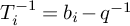
$T_i=b_i-q$
 and
$T_i^{-1}=b_i-q^{-1}$
 , for every
$i\in \widehat {I}$
 . The Kazhdan–Lusztig basis is given by
$\{\rho ^m b_w \mid m\in \mathbb {Z}, w \in \widehat {\mathfrak {S}}_n \}$
 , where the definition of
$b_w$
 requires the choice of a rex for w but is independent of that choice.
For
$n=1$
 , the (non-extended) affine Hecke algebra
$\widehat {H}_1$
 is the trivial one-dimensional algebra isomorphic to
$\mathbb {Z}[q,q^{-1}]$
 . For
$n\geq 2$
 , the (non-extended) affine Hecke algebra
$\widehat {H}_n$
 is the subalgebra of
$\widehat {H}^{ext}_n$
 generated by either
$T_i$
 or
$b_i,$
 for
$ i\in \widehat {I}$
 .
For
$n=1$
 , the finite Hecke algebra
$H_1$
 is also the trivial one-dimensional algebra isomorphic to
$\mathbb {Z}[q,q^{-1}]$
 . For
$n\geq 2$
 , the finite Hecke algebra
$H_n$
 is the
$\mathbb {Z}[q,q^{-1}]$
 -subalgebra of
$\widehat {H}_n$
 generated by either
$T_i$
 or
$b_i$
 , for
$i\in I$
 .
There is a third presentation of
$\widehat {H}^{ext}_n$
 , called the Bernstein presentation. In that presentation,
$\widehat {H}^{ext}_n$
 is defined as a twisted tensor product of
$H_n$
 and the algebra of Laurent polynomials in n indeterminates with coefficients in
$\mathbb {Z}[q,q^{-1}]$
 . There are several possible choices for defining the commutation relations. The one we use here has indeterminates
$y_1,\dotsc , y_n$
 , with relations given by

for
$i\in I$
 .
The relation between this Bernstein presentation and our first presentation of
$\widehat {H}^{ext}_n$
 is given by


Remark 2.1. Some remarks about the various conventions in the literature are in order. We try to follow conventions close to those in [Reference EliasEli2]. Our presentation of the extended affine Hecke algebra in Section 2.1 agrees with [Reference EliasEli2], as does the relation between the standard generators and the Kazhdan–Lusztig generators.
The standard trace
$\epsilon \colon \widehat {H}^{\mathrm {ext}}_{n}\to \mathbb {Z}[q,q^{-1}]$
 , which also plays an important role in this paper, is the
$\mathbb {Z}[q,q^{-1}]$
 -linear map defined by

for
$r\in \mathbb {Z}$
 and
$w\in \widehat {\mathfrak {S}}_n$
 , where
$\delta _{-,-}$
 is the Kronecker delta. The trace induces a q-sesquilinear form
$(-,-)$
 on
$\widehat {H}^{\mathrm {ext}}_{n}$
 defined by

where
$\omega $
 is the q-antilinear antiinvolution on
$\widehat {H}^{\mathrm {ext}}_{n}$
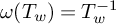
 defined by
$\omega (\rho )=\rho ^{-1}$
 and
$\omega (T_w)=T_{w}^{-1}$
 , for
$w\in \widehat {\mathfrak {S}}_n$
 . By definition, q-sesquilinear means that
$(-,-)$
 is
$\mathbb {Z}$
 -bilinear and satisfies
$(qx,y)=q^{-1}(x,y)=(x,q^{-1}y)$
 , for all
$x,y\in \widehat {H}^{\mathrm {ext}}_{n}$
 . The above definitions imply that
$\omega (b_w)=b_{w^{-1}}$
 and that the Kazhdan–Lusztig basis is asymptotically orthonormal w.r.t.
$(-,-)$
 , see e.g. [Reference Elias, Makisumi, Thiel and WilliamsonEMTW, Theorem 3.21] for non-extended affine type A.
Theorem 2.2. For all
$k,l\in \mathbb {Z}$
 and
$u,v\in \widehat {\mathfrak {S}}_n$
 , we have
$\left (\rho ^k b_u,\rho ^l b_v \right )=\delta _{k,l}\left (b_u,b_v \right )$
 and

2.2 The embedding
Let
$1\leq k\leq n-1$
 . There are two unital embeddings of
$\mathbb {Z}[q,q^{-1}]$
 -algebras
$\psi _L\colon \widehat {H}^{\mathrm {ext}}_{k}\to \widehat {H}^{\mathrm {ext}}_{n}$
 (the left embedding) and
$\psi _R\colon \widehat {H}^{\mathrm {ext}}_{n-k} \to \widehat {H}^{\mathrm {ext}}_{n}$
 (the right embedding), which are easily defined in terms of the Bernstein presentation:

The two embeddings give rise to a
$\mathbb {Z}[q,q^{-1}]$
 -linear map

defined by

By definition,
$\psi _{k,n-k}(a \otimes 1)=\psi _L(a)$
 and
$\psi _{k,n-k}(1 \otimes b)=\psi _R(b)$
 , where we denote the identity element of the various Hecke algebras by the same symbol
$1$
 .
It is easy to see that this map is a homomorphism of algebras. Note that
$\psi _L$
 and
$\psi _R$
 form a commuting pair of algebra homomorphisms, in the sense that

holds for all
$a\in \widehat {H}^{\mathrm {ext}}_{k}, b\in \widehat {H}^{\mathrm {ext}}_{n-k}$
 , because the
$y_m$
 for
$1\leq m\leq n$
 all commute with each other and we have
$T_i T_j=T_j T_i$
 ,
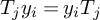
$T_iy_j=y_jT_i$
 and
$T_jy_i=y_iT_j$
 for all
$1\leq i\leq k-1$
 and
$k+1\leq j\leq n-1$
 . Therefore, for all
$a_1,a_2\in \widehat {H}^{\mathrm {ext}}_{k}$
 and
$b_1,b_2\in \widehat {H}^{\mathrm {ext}}_{n-k}$
 , we have

which means that

Using (14) to translate to the presentation in terms of the standard generators and
$\rho $
 given in (8) and (9), yields


and


where we use the notation
${\rho _{\color {blue}L}}$
 and
${\rho _{\color {purple}R}}$
 for the twist generators of
$\widehat {H}^{\mathrm {ext}}_{k}$
 and
$\widehat {H}^{\mathrm {ext}}_{n-k}$
 , with
$\rho $
 being used for the generator of
$\widehat {H}^{\mathrm {ext}}_{n}$
 . The underscript letters
$\color {blue}L$
 and
$\color {purple}R$
 are meant to signify “
${\color {blue}{\text {left}}}$
 ” and “
${\color {purple}{\text {right}}}$
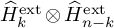
 ” to match their position in the tensor product
$\widehat {H}^{\mathrm {ext}}_{k}\otimes \widehat {H}^{\mathrm {ext}}_{n-k}$
 .
Since
$\psi _L({\rho _{\color {blue}L}})$
 and
$\psi _R({\rho _{\color {purple}R}})$
 commute, we have

The image of the Kazhdan–Lusztig generators under
$\psi _L$
 and
$\psi _R$
 is

Using (19) and (21) it follows at once that

2.3 Diagrammatics
As is well known, the various Hecke algebras described above also have a diagrammatic incarnation, since all of them can be defined as a quotient of the group algebra of the corresponding braid group. In this incarnation, the standard generators correspond to crossings between two neighbouring strands. In the affine case, we have to use braid diagrams on a cylinder, which we depict as a rectangle where the two vertical boundary components are identified. In this diagrammatic presentation for
$\widehat {H}^{\mathrm {ext}}_{n}$
 we have

where
$i=1,\dotsc ,n-1$
 . Note that we do not draw all the vertical lines and that the boundary points at the top, resp. at the bottom, of the braid diagram are cyclically ordered. In our planar presentation we always order them from left to right starting with
$1$
 and ending with n. In our conventions, the product
$XY$
 consists of gluing the diagram of X atop the one of Y.
The embedding
$\psi _{k,n-k}$
 can also be described diagrammatically in a natural way. The diagram for
$\psi _{k,n-k}(X\otimes Y)$
 consists of placing the cylinder with the diagram for
$Y\in \widehat {H}^{\mathrm {ext}}_{n-k}$
 inside the cylinder with the diagram for
$X\in \widehat {H}^{\mathrm {ext}}_{k}$
 and then projecting the outer cylinder over the inner in such a way that the boundary points of the diagram for X are sent to themselves, while the boundary points of the diagram for Y are sent to the points labelled
$k+1,\dotsc , n$
 . This is easily visualised using coloured diagrams: we use
$\color {blue}{\text {blue}}$
 for the diagrams of the elements of
$\widehat {H}^{\mathrm {ext}}_{k}$
 and
$\color {purple}{\text {purple}}$
 for the ones of
$\widehat {H}^{\mathrm {ext}}_{n-k}$
 . In this convention, the cylinder with a purple diagram goes inside the one with the blue diagram.

Example 2.3. The diagrams for
$\psi _L({\rho _{\color {blue}L}})=\psi _{k,n-k}({\rho _{\color {blue}L}}\otimes 1)$
 and
$\psi _R({\rho _{\color {purple}R}})=\psi _{k,n-k}(1\otimes {\rho _{\color {purple}R}})$
 :

Example 2.4 (Diagrams on a cylinder).
To visualize this product, it might help to draw the inclusions from Example 2.3 using diagrams on a cylinder. For the curious reader we have also drawn the diagram for the Bernstein generator
$y_1$
 .

The Bernstein generator
$y_1$
 can be drawn as

Note that the equation
$\psi _{k,n-k}({\rho _{\color {blue}L}}\otimes 1)\psi _{k,n-k}(1\otimes {\rho _{\color {purple}R}})=\psi _{k,n-k}(1\otimes {\rho _{\color {purple}R}})\psi _{k,n-k}({\rho _{\color {blue}L}}\otimes 1)$
 translates to “
$\color {blue}{\text {blue}}$
 ” and
$\color {purple}{\text {purple}}$
 sliding past each other in the corresponding compositions of the diagrams above.
3 Rouquier–Soergel calculus
3.1 Soergel calculus in extended affine type A and Rouquier complexes
In this section, we initially revisit the definition of the diagrammatic Soergel category for the extended affine type A as presented in [Reference Mackaay and ThielMaTh] (see also [Reference Mackaay, Miemietz and VazMMV] and [Reference EliasEli2]).
Let
$\mathbb {k}$
 be an arbitrary field. Our conventions for graded (
$\mathbb {k}$
 -linear additive) categories and shifts are as in [Reference Mackaay, Miemietz and VazMMV, §3.1], which match those of [Reference Elias, Makisumi, Thiel and WilliamsonEMTW, Section 4.1]. Since those conventions are important, let us briefly recall them. Throughout this paper, graded will always mean
$\mathbb {Z}$
 -graded. For any
$t\in \mathbb {Z}$
 , the grading shift
$\langle t\rangle $
 of a graded vector space
$M\cong \oplus _{a\in \mathbb {Z}} M_a$
 is defined by
$(M\langle t\rangle )_a:=M_{a+t}$
 for all
$a\in \mathbb {Z}$
 . This implies that
$\mathrm {hom}(M\langle r\rangle , N\langle t\rangle )$
 consists of all homogeneous linear maps between M and N of degree
$t-r$
 . The graded morphism space of all morphisms from M to N is defined as
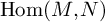
$\mathrm {Hom}(M,N):=\oplus _{t\in \mathbb {Z}} \mathrm {hom}(M,N\langle t\rangle )$
 . In the categories of this paper, the objects need not be vector spaces, in which case the grading shifts are formal, but the morphism spaces are always vector spaces consisting of (equivalence classes of) linear combinations of diagrams. Each diagram has some degree
$s\in \mathbb {Z}$
 and can therefore be seen as a morphism between two objects with shifts
$M\langle r\rangle $
 and
$N\langle t\rangle $
 , such that
$s=t-r$
 , or as a homogeneous morphism between M and N of degree
$s=t-r$
 . To distinguish a non-graded category
$\mathcal {C}$
 with shift and lower case morphism spaces of the form
$\mathrm {hom}(M\langle r \rangle ,N\langle t\rangle )$
 from the associated graded category with morphism spaces of the form
$\mathrm {Hom}(M,N)$
 , we denote the latter by
$\mathcal {C}^*$
 .
Recall that the additive envelope of a
$\mathbb {k}$
 -linear category
$\mathcal {C}$
 is the additive, linear category
$\mathcal {C}_{\oplus }$
 whose objects are formal direct sums of objects in
$\mathcal {C}$
 and whose morphisms are matrices of morphisms in
$\mathcal {C}$
 , such that composition is given by matrix multiplication. The Karoubi envelope of an additive, linear category is a formal enhancement which results in an idempotent complete category we denote
$\mathcal {C}_{\oplus , e}$
 . For more information on these formal constructions, see e.g. [Reference Elias, Makisumi, Thiel and WilliamsonEMTW, Sections 11.2.2 – 11.2.4].
3.1.1 Soergel calculus in extended affine type A
The diagrammatic Bott-Samelson category of extended type
$\widehat {A}_{n-1}$
 , denoted
$\widehat {\mathscr {BS}}^{\mathrm {ext}}_n$
 , is the
$\mathbb {Z}$
 -graded,
$\mathbb {R}$
 -linear, pivotal category whose objects are grading shifts of finite words in the alphabet
$\widehat {I}\cup \{\pm \}$
 , and whose vector spaces of morphisms are defined below in terms of generating diagrams and relations. Recall that a pivotal category is a monoidal category with duals satisfying certain conditions, see [Reference Etingof, Gelaki, Nikshych and OstrikEGNO, Definition 4.7.8]. We will often identify that alphabet with the corresponding elementary Soergel bimodules
$\{{\mathrm {B}}_i,i\in \widehat {I}\}\cup \{{\mathrm {B}}_{\rho }^{\pm 1} \}$
 , which is justified by [Reference Mackaay and ThielMaTh, Theorem 2.10]. These are bimodules over a polynomial algebra R, defined below (47). Under this identification, a word in the alphabet corresponds to a tensor product of
${\mathrm {B}}_i$
 and
$\mathrm {B}_\rho $
 , which is called a Bott-Samelson bimodule. The empty word is the identity object, which is identified with R. The tensor product is taken over R, but we will often suppress
$\otimes _R$
 in our notation, e.g., we will simply write
$\mathrm {B}_1 \mathrm {B}_2$
 for
$\mathrm {B}_1\otimes _R \mathrm {B}_2$
 . The diagrams then then correspond to R-R-bimodule maps, but we will not use those maps explicitly in this paper. As explained above, the diagrams can be seen as morphisms between degree-shifted objects or as homogeneous morphisms between unshifted objects. In this definition, we take the former point of view. As explained above, the graded version of
$\widehat {\mathscr {BS}}^{\mathrm {ext}}_n$
 will be denoted by
$\widehat {\mathscr {BS}}^{\mathrm {ext},*}_n$
 .
The identity morphism on
$i\in \widehat {I}$
 is given by a vertical non-oriented strand coloured by i, whereas the identity morphism on
$+/-$
 is given by a vertical upward/downward oriented black strand. As usual, we will colour the unoriented strands to facilitate the reading of the diagrams. When there are too many different colours in a diagram, the colours are sometimes indicated by labels next to the strands. We say that two colours
$i,j\in \widehat {I}$
 are adjacent if
$i \equiv j\pm 1\bmod n$
 and that they are distant otherwise.
The number of different types of diagram increases with n, so below we first give the generating diagrams for
$n\geq 1$
 , then the additional ones for
$n\geq 2$
 and, finally, the additional ones that only show up for
$n\geq 3$
 .
-
• For $n\geq 1$
 , (23)
and the corresponding oriented black caps.
-
• For $n\geq 2$
, with
$i\in \widehat {I}$
, (24)and the diagrams obtained from these by a rotation of $180$
degrees (which have the same degrees). -
• For $n\geq 3$
, with
$i,j,k\in \widehat {I}$
such that
$\vert i-j\vert =1$
and
$\vert i-k\vert>1$
, (25)and the diagrams obtained from these by a rotation of $180$
degrees (which have the same degrees).


We read diagrams from bottom to top as morphisms, i.e., their source is at the bottom and their target at the top.
Diagrams can be stacked vertically (composition of morphisms) and juxtaposed horizontally (monoidal product of morphisms), while adding the degrees, and are subject to the relations below. The list contains all relations for all
$n\geq 1$
 , but for
$n=1$
 and
$n=2$
 only the relations involving the respective generators should be considered. For
$n=2$
 , there is an additional subtlety in (37), as indicated. We also assume isotopy invariance and cyclicity, meaning that closed parts of the diagrams can be moved around freely in the plane as long as they do not cross any other strands and the boundary is fixed, and all diagrams can be bent and rotated, and the bent and rotated versions of the relations also hold.
-
• Relations involving only one colour:
(26)(27)(28)(29) -
• Relations involving two distant colours:
(30)(31)(32)(33) -
• Relations involving two adjacent colours:
(34)(35)(36)(37) -
• Relation involving three distant colours:
(38) -
• Relation involving two adjacent colours and one distant from the other two:
(39) -
• Relation involving three colours such that i is adjacent to j, and j is adjacent to k:
(40)


-
• Relations involving only oriented strands:
(41)(42) -
• Relation involving oriented strands and two distant coloured strands:
(43) -
• Relations involving oriented strands and two adjacent coloured strands:
(44)(45)(46) -
• Relations involving oriented strands and three adjacent coloured strands:
(47)


Remark 3.1. Further relations that are consequences of (37) usually have two cases too, e.g.

and similarly with the two colours switched.
Note that the empty word is the identity object in
$\widehat {\mathscr {BS}}^{\mathrm {ext}}_n$
 and its endomorphisms are the closed diagrams, which by the relations above are equal to polynomials in the coloured dumbbells

As each dumbbell has degree
$2$
 , the degree of any polynomial in these dumbbells, as a morphism in
$\widehat {\mathscr {BS}}^{\mathrm {ext}}_n$
 , is twice its polynomial degree. From now on, we denote this polynomial algebra by R.
Note further that, by relations (29), (37) and (33), the morphism
$\fbox {y}$
 , defined in [Reference Mackaay and ThielMaTh] by

is central, in the sense that it can be slid through all diagrams (i.e. it commutes horizontally with all morphisms), because it is equal to the sum of all simple roots.
Definition 3.2. The extended Soergel category
$\widehat {\mathscr {S}}^{\mathrm {ext}}_n$
 is the Karoubi envelope of the additive envelope of
$\widehat {\mathscr {BS}}^{\mathrm {ext}}_n$
 .
Note that in our definition shifts are already part of
$\widehat {\mathscr {BS}}^{\mathrm {ext}}_n$
 and recall that the idempotent complete category
$\widehat {\mathscr {S}}^{\mathrm {ext}}_n$
 is Krull-Schmidt, see e.g. [Reference Elias, Makisumi, Thiel and WilliamsonEMTW, Section 11.2.3]. It therefore makes sense to consider the split Grothendieck group
$[\widehat {\mathscr {S}}^{\mathrm {ext}}_n]_{\oplus }$
 , which has a natural
$\mathbb {Z}[q,q^{-1}]$
 -module structure defined by
$[\mathrm {X}\langle 1\rangle ]=:q[\mathrm {X}]$
 , for every object
$\mathrm {X}\in \widehat {\mathscr {S}}^{\mathrm {ext}}_n$
 . It also has a natural algebra structure, inherited from the monoidal structure on
$\widehat {\mathscr {S}}^{\mathrm {ext}}_n$
 .
Finally, let us recall the Soergel categorification theorem, see e.g. [Reference Mackaay and ThielMaTh, Theorem 2.5] for extended affine type A (which was based on previous results by Härterich) and [Reference Elias, Makisumi, Thiel and WilliamsonEMTW, Theorem 11.1] for general Coxeter type. For every
$w\in \widehat {\mathfrak {S}}_n$
 , choose a rex
$\underline {w}=(s_{i_1},\ldots , s_{i_l})$
 and define the Bott-Samelson bimodule

There is an essentially unique indecomposable summand
${\mathrm {B}}_w\in \widehat {\mathscr {S}}^{\mathrm {ext}}_n$
 of
$\mathrm {BS}(\underline {w})$
 that is not a summand of
$\mathrm {BS}(\underline {u})$
 for any
$u\prec w$
 in
$\widehat {\mathfrak {S}}_n$
 , where
$\prec $
 is the Bruhat order. The isomorphism class of
${\mathrm {B}}_w$
 does not depend on the choice of rex for w. More generally, for any
$k\in \mathbb {Z}$
 and any
$w\in \widehat {\mathfrak {S}}_n$
 , the object
${\mathrm {B}}_\rho ^k {\mathrm {B}}_w$
 is indecomposable in
$\widehat {\mathscr {S}}^{\mathrm {ext}}_n$
 and the set of these indecomposables is complete and irredundant, meaning that they are all mutually non-isomorphic and every indecomposable in
$\widehat {\mathscr {S}}^{\mathrm {ext}}_n$
 is isomorphic to one of them up to grading shift. Recall further that
$\widehat {H}^{\mathrm {ext}}_{n}$
 has a q-sesquilinear form
$(-,-)$
 , see (17). Similarly,
$[\widehat {\mathscr {S}}^{\mathrm {ext}}_n]_{\oplus }$
 has a q-sesquilinear form
$\langle -,-\rangle $
 , called the graded Euler form. To define it, one has to recall that the morphism spaces in
$\widehat {\mathscr {S}}^{\mathrm {ext},*}_n$
 are free as left and as right graded R-modules and that their graded rank is finite and does not depend on whether we consider them as left or as right R-modules. By definition, the value of
$\langle [X], [Y] \rangle $
 , for
$X,Y\in \widehat {\mathscr {S}}^{\mathrm {ext}}_n$
 , is equal to the graded rank of
$\mathrm {Hom}_{\widehat {\mathscr {S}}^{\mathrm {ext},*}_n}(X,Y)$
 . The following theorem combines Soergel’s categorification theorem and Soergel’s conjecture (which has been proved, see [Reference Mackaay and ThielMaTh] and references therein).
Theorem 3.3. The
$\mathbb {Z}[q,q^{-1}]$
 -linear map

is an isomorphism of
$\mathbb {Z}[q,q^{-1}]$
 -algebras intertwining the two q-sesquilinear forms.
This intertwining property goes under the name of Soergel’s hom formula and will be used several times in Section 5.3, so let us state it explicitly here:

for all
$k,l\in \mathbb {Z}$
 and all
$u,v\in \widehat {\mathfrak {S}}_n$
 , where
$\underline {\mathrm {rk}}$
 denotes the graded rank.
3.1.2 Rouquier complexes
We give a summary of the material in [Reference Mackaay, Miemietz and VazMMV, §4.1] that is needed in the sequel. In particular, we introduced a diagrammatic calculus for certain morphisms between tensor products of Rouquier complexes and Bott–Samelson bimodules in finite type A. In the summary below, we recall the basic features of that calculus, generalising it to extended affine type A as well. Note that it only describes part of the morphism spaces in
$K^b(\widehat {\mathscr {S}}^{\mathrm {ext}}_n)$
 , which are not yet understood in full generality. Describing the homotopy categories of Rouquier complexes in terms of generators and relations is a hard problem, even in finite type A, see for example [Reference Libedinsky and WilliamsonLiWi].
Throughout the rest of the paper, if
$\mathcal {C}$
 is a
$\mathbb {k}$
 -linear, additive category, for any field
$\mathbb {k}$
 , we write
$C^b(\mathcal {C})$
 for the category of bounded complexes in
$\mathcal {C}$
 and
$K^b(\mathcal {C})$
 for its homotopy category. If
$\mathcal {C}$
 is also monoidal, then the usual monoidal product of chain complexes equips
$K^b(\mathcal {C})$
 with a monoidal structure as well. If
$\mathcal {C}$
 is also graded, then
$K^b(\mathcal {C})$
 is bigraded and we denote the shift inherited from
$\mathcal {C}$
 by
$\langle \cdot \rangle $
 and the homological shift by
$[\cdot ]$
 .
For
$n\geq 2$
 , the Rouquier complexes
${\mathrm {T}}_i^{\pm 1}\in K^b(\widehat {\mathscr {S}}^{\mathrm {ext}}_n)$
 for
$i\in \widehat {I}$
 are defined by

with
${\mathrm {B}}_i$
 placed in homological degree zero in both complexes.
The identity morphisms of
${\mathrm {T}}_i^{\pm 1}$
 are depicted by

All generators in (51), (55) and (56) below have degree zero with respect to both gradings.
-
• The 1-colour generators are the cups and caps:
(51)The following lemma recalls the content of [Reference Mackaay, Miemietz and VazMMV, Lemma 4.4].
Lemma 3.4. For any $\color {blue}{i}\in \widehat {I}$
, we have the following relations between morphisms in
$K^b(\widehat {\mathscr {S}}^{\mathrm {ext}}_n)$
: (52)(53)(54)For the diagrams and relations given in the rest of this section there are also similar diagrams and relations involving inverses of Rouquier complexes.
For $n>2$
, there are additional diagrams and relations. -
• The six-valent vertices for $\color {blue}{i}$
and
$\color {myred}{j}$
adjacent: (55)Note that a solid strand corresponds to the identity on a Soergel bimodule, whereas a dashed strand corresponds to the identify morphism on a Rouquier complex, and all morphisms are defined in the homotopy category. These satisfy
-
• The crossings for $\color {blue}{i}$
and
$\color {orange}{k}$
distant: (56)These satisfy


3.2 More diagrammatic shortcuts for Rouquier complexes
We now develop some new diagrammatics to handle morphisms between tensor products of Soergel bimodules and Rouquier complexes.
For any
$a,b\in \mathbb {Z}$
 define

where the indices on the right-hand side can be shifted modulo n so that they belong to
$\widehat {I}=\{0,1,\ldots , n-1\}$
 . For example, we have
${\mathrm {T}}_{[-2,2]}={\mathrm {T}}_{n-2}{\mathrm {T}}_{n-1}{\mathrm {T}}_0\mathrm {T}_1\mathrm {T}_2$
 . Of course, the above notation is not unique, since
$\mathrm {T}_{[a,b]}=\mathrm {T}_{[a+kn,b+kn]}$
 for any
$a,b,k\in \mathbb {Z}$
 , but we trust that this does not cause any confusion. Note that in general
$\mathrm {T}_{[a,b]}\ne \mathrm {T}_{[a+kn,b+ln]}$
 if
$k\ne l$
 , e.g.,
${\mathrm {T}}_{[0,1]}={\mathrm {T}}_0\mathrm {T}_1$
 while
$\mathrm {T}_{[n,1]}=\mathrm {T}_0 \mathrm {T}_{n-1}\cdots \mathrm {T}_1$
 , which are different when
$n>2$
 . Observe that it is important that the indices
$a,b$
 in
$\mathrm {T}_{[a,b]}$
 be integers and not residue classes modulo n, because that allows for products of
$\mathrm {T}_i$
 whose length is greater than n, e.g., e.g.,
${\mathrm {T}}_{[0,2n-1]}={\mathrm {T}}_0{\mathrm {T}}_1\cdots {\mathrm {T}}_{n-1}{\mathrm {T}}_0{\mathrm {T}}_1\cdots {\mathrm {T}}_{n-1}$
 .
Using the same conventions, we introduce the identity morphism on
${\mathrm {T}}_{[a,b]}$
 by

The unit and counit of the adjunction between
${\mathrm {T}}_{[a,b]}$
 and its inverse are drawn as a cup and a cap, respectively, and these satisfy the usual isotopy and invertibility relations (cf. [Reference Mackaay, Miemietz and VazMMV, Lemma 4.4, Lemma 4.15]). Cups and caps have degree zero, as do the generators in (60), (64), (67), (70), (62), (76) and (79).
Lemma 3.5. For any
$a,b\in \mathbb {Z}$
 , we have the following relations between morphisms in
$K^b(\mathscr {S}_n)$
 :


It is useful to introduce mergers and splitters

for
$c>b\geq a$
 , realising the equalities of chain complexes
${\mathrm {T}}_{[a,b]}{\mathrm {T}}_{[b+1,c]}={\mathrm {T}}_{[a,c]}$
 (and analogously for their inverses). By definition, they satisfy

Of course, similar mergers and splitters can be defined for
$a\geq b> c$
 , where
$[a,c]$
 is subdivided into
$[a,b]$
 and
$[b-1,c]$
 . Further, one can use cups and caps to define generators like

satisfying the obvious relations in
$K^b(\mathscr {S}_n)$
 .
Lemma 3.6. The following equations hold in
$K^b(\widehat {\mathscr {S}}^{\mathrm {ext}}_n)$
 :

Proof. An easy computation using [Reference Mackaay, Miemietz and VazMMV, Lemma 4.6].
The chain complexes
$B_\rho ^{-1}{\mathrm {T}}_{[a,b]}$
 and
${\mathrm {T}}_{[a-1,b-1]}B_\rho ^{-1}$
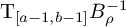 are isomorphic. This is an easy consequence of the isomorphism of the chain complexes
$B_\rho ^{-1}{\mathrm {T}}_{k}\cong {\mathrm {T}}_{k-1}B_\rho ^{-1}$
 , which follows from (44). This homotopy equivalence and its variants are represented by the diagrams

satisfying the relations (which are easy consequences of (44))

We assume that
$n>2$
 until the end of this section. We say that
$[a,b]$
 and
$[c,d]$
 are distant if every index appearing in
${\mathrm {T}}_{[a,b]}$
 is distant from every index in
${\mathrm {T}}_{[c,d]}$
 . In this case the chain complexes
${\mathrm {T}}_{[a,b]}\mathrm {T}_{[c,d]}^{\pm 1}$
 and
$\mathrm {T}_{[c,d]}^{\pm 1}\mathrm {T}_{[a,b]}$
 are isomorphic, with the isomorphism being given by diagrams like

which satisfy the relations in
$K^b(\widehat {\mathscr {S}}^{\mathrm {ext}})$
 given below, for mutually distant
$[a,b]$
 ,
$[c,d]$
 and
$[e,f]$
 and with any of the possible orientations

and (together with its variants)

When
$k=[k,k]$
 is distant from
$[a,b]$
 , the chain complexes
${\mathrm {B}}_k{\mathrm {T}}_{[a,b]}$
 and
${\mathrm {T}}_{[a,b]}{\mathrm {B}}_k$
 are homotopy equivalent and the homotopy equivalence can be represented by the diagram by the diagram

satisfying the relations

and its variants. If
$[a,b]$
 is distant from i, j and k, and j is adjacent to i but distant from k, we also have

For
$0<a,b<n$
 the chain complex
${\mathrm {T}}_{[a,b]}B_k$
 is homotopy equivalent to
$B_{k-1}{\mathrm {T}}_{[a,b]}$
 when
$b<k\leq a$
 , and homotopy equivalent to
$B_{k+1}{\mathrm {T}}_{[a,b]}$
 when
$a\leq k<b$
 (note that
$a\neq b$
 ). This is proved in the same way as [Reference Mackaay, Miemietz and VazMMV, Lemma 4.11]. The homotopy equivalences are realised by the following family of diagrams

satisfying the relations


and their variants. Relations (71) are immediate, while the relations in the remaining two lines are proved as in [Reference Mackaay, Miemietz and VazMMV, Lemmas 4.18 and 4.21], respectively.
To prove the next lemma we will use the hom & dot trick. Due to its extensive use in the next section, we will briefly explain it in the following remark.
Remark 3.7 (The hom & dot trick).
Let A and B be two non-zero diagrams in a given morphism space. If the latter space is one-dimensional, then
$A=\lambda B$
 , where
$\lambda $
 is a non-zero scalar. To prove that
$\lambda =1$
 we will often attach dots to certain endpoints of A and B and simplify the resulting diagrams so that they can be easily compared.
Lemma 3.8. For
$a,b,c\in \mathbb {Z}$
 such that c is distant from
$[a,b]$
 , the following relations hold in
$K^b(\widehat {\mathscr {S}}^{\mathrm {ext}}_n)$
 :

Proof. We use the hom & dot trick. By using cups and caps, both diagrams can be deformed to morphisms of degree zero from
${\mathrm {B}}_{c+1}$
 to
${\mathrm {B}}_\rho {\mathrm {T}}_{[a,b]}{\mathrm {B}}_c{\mathrm {B}}_\rho ^{-1}{\mathrm {T}}_{[a\!+\!1,b\!+\!1]}^{-1}$
 , which is homotopy equivalent to
${\mathrm {B}}_{c+1}$
 because

Soergel’s hom formula in (49) implies that the space of degree-preserving endomorphisms of
${\mathrm {B}}_{c+1}$
 (either in
$\widehat {\mathscr {S}}^{\mathrm {ext}}_n$
 or in
$K^b(\widehat {\mathscr {S}}^{\mathrm {ext}}_n)$
 ) is one-dimensional, so the two deformed diagrams are non-zero multiples of each other, which implies that the same holds for the two diagrams in (74). Attaching a dot to one of the free ends of the non-oriented strand we see that these morphisms are equal.
Of course, there are other variants of (74) with, for example, other orientations, or involving one oriented black strand and two thick oriented strands. Note that we can even relax the condition that c is distant from
$[a,b]$
 . We leave the details to the reader.
Until the end of this subsection, assume that
$a,b\in \mathbb {Z}$
 such that
$a<b$
 . By applying [Reference Mackaay, Miemietz and VazMMV, Lemma 4.8] recursively, one obtains a homotopy equivalence

The corresponding isomorphism in
$K^b(\widehat {\mathscr {S}}^{\mathrm {ext}}_n)$
 and its inverse are represented by the diagrams

satisfying the relations

in
$K^b(\widehat {\mathscr {S}}^{\mathrm {ext}})$
 . There is a similar homotopy equivalence

and the corresponding isomorphism in
$K^b(\widehat {\mathscr {S}}^{\mathrm {ext}}_n)$
 and its inverse are represented by the diagrams

satisfying relations analogous to those in (77).
Remark 3.9. One needs to be careful with the use of the colours of the strands in the diagrams in (76) and (79). For example, the definition of
$\Psi _R$
 in Section 4.1.2 contains the diagram

for
$0<k<n$
 . To compare the labels of this diagram with the conventions in (79), one needs to use the equality

However, there is no homotopy equivalence given by a diagram of the form

because that would imply that
$a=n-1$
 and
$b=k-1$
 in (79), violating our assumption that
$a<b$
 .
Proceeding as in the proof of [Reference Mackaay, Miemietz and VazMMV, Lemma 4.25], one can show that the following holds in
$K^b(\widehat {\mathscr {S}}^{\mathrm {ext}})$
 :

For k distant from
$[a,b]$
 , it is easy to see that

Lemma 3.10. We have the following in
$K^b(\widehat {\mathscr {S}}^{\mathrm {ext}})$
 :

Proof. We use the hom & dot trick. By using cups and caps, both diagrams are isotopic to diagrams realising morphisms from
${\mathrm {T}}_{[b-1,a]}^{-1}{\mathrm {B}}_b{\mathrm {T}}_{[b-1,a]}$
 to
${\mathrm {T}}_{[b,a+1]}{\mathrm {B}}_a{\mathrm {B}}_a{\mathrm {T}}_{[b,a+1]}^{-1}$
 . Gluing the second diagram in (76) at the bottom results in two morphisms of degree
$-1$
 from
${\mathrm {T}}_{[b,a+1]}{\mathrm {B}}_a{\mathrm {T}}_{[b,a+1]}^{-1}$
 to
${\mathrm {T}}_{[b,a+1]}{\mathrm {B}}_a{\mathrm {B}}_a{\mathrm {T}}_{[b,a+1]}^{-1}$
 . By biadjointness and the invertibility of
${\mathrm {T}}_{[b,a+1]}$
 in
$K^b(\widehat {\mathscr {S}}^{\mathrm {ext}}_n)$
 , there is a canonical isomorphism

The latter isomorphism follows from Soergel’s hom formula in (49) and the fact that
${\mathrm {B}}_a {\mathrm {B}}_a\cong {\mathrm {B}}_a\langle 1\rangle \oplus {\mathrm {B}}_a\langle -1\rangle $
 . By attaching dots to the free top ends labelled a in (82) and using (80) and (27), one sees that they are equal.
Lemma 3.11. For c distant from
$[b,a]$
 , we have


in
$K^b(\widehat {\mathscr {S}}^{\mathrm {ext}})$
 .
Proof. We use the hom & dot trick again and only prove (83), (84) being similar. As in the proof of Lemma 3.8, first apply cups and caps to get two degree preserving morphisms from
${\mathrm {T}}_{[b-1,a]} {\mathrm {T}}_{[b,a+1]} {\mathrm {B}}_c {\mathrm {B}}_a {\mathrm {T}}_{[b,a+1]}^{-1}{\mathrm {T}}_{[b-1,a]}^{-1}$
 to
${\mathrm {B}}_b{\mathrm {B}}_c$
 , then use the homotopy equivalences

and the fact that
${\mathrm {B}}_b {\mathrm {B}}_c\cong {\mathrm {B}}_{bc}$
 , which implies that
$\hom _{\widehat {\mathscr {S}}^{\mathrm {ext}}_n}({\mathrm {B}}_{bc}, {\mathrm {B}}_{bc})$
 is one-dimensional by Soergel’s hom formula in (49). We attach dots to the upper boundary points labelled b and c of the two diagrams in (83) and show that the resulting diagrams are equal using (80) and (27).
4 Parabolic embedding: categorified story
4.1 The categorical embedding
Let
$k,n\in \mathbb {Z}$
 such that
$0<k<n$
 . In this section we are going to define a monoidal,
$\mathbb {R}$
 -linear functor

categorifying the embedding
$\psi _{k,n-k}$
 of algebras from Secton 2.2, but before giving the definition in Section 4.1.2, we first explain the general idea behind it.
4.1.1 Symmetric pairs of monoidal functors
The content of this subsection must be known to experts, but we do not know of any reference in the literature for what we call a symmetric pair of monoidal functors in Definition 4.2. We thank Robert Laugwitz for pointing out to us that our definition can be reformulated in terms of the Drinfeld centralisers of the monoidal functors, as we will briefly explain in Remark 4.3. Since we claim no originality in this subsection and it is only meant to help the reader understand our construction of
$\Psi _{k,n-k}$
 , we have not endeavored to formulate the abstract notions and results in the most general setting.
As for the terminology, we call a monoidal category or functor strict monoidal if the coherence morphisms of the monoidal structure are identities, otherwise we simply call it monoidal. However, we should warn the reader that we treat canonical natural isomorphisms, such as the unitors and associators of
$\times , \otimes $
 and
$\oplus $
 , as identities. With this harmless simplification, the categories
$\widehat {\mathscr {S}}^{\mathrm {ext}}_k\boxtimes \widehat {\mathscr {S}}^{\mathrm {ext}}_{n-k}$
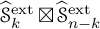 and
$K^b(\widehat {\mathscr {S}}^{\mathrm {ext}}_n)$
 are considered to be strict monoidal. However, our monoidal functor
$\Psi _{k,n-k}$
 is definitely not strict, as will see in Section 4.2.3.
In this more abstract subsection, we work over an arbitrary field
$\mathbb {k}$
 . Recall that, for
$\mathbb {k}$
 -linear categories
$\mathcal {C}$
 and
$\mathcal {D}$
 , their tensor product
$\mathcal {C}\diamond \mathcal {D}$
 is the
$\mathbb {k}$
 -linear category with
$\mathrm {Ob}(\mathcal {C}\diamond \mathcal {D})=\mathrm {Ob}(\mathcal {C})\times \mathrm {Ob}(\mathcal {D})$
 and morphism spaces
$\mathrm {Hom}_{\mathcal {C}\diamond \mathcal {D}}\big ((\mathtt {i},\mathtt {j}),(\mathtt {k},\mathtt {l})\big )=\mathrm {Hom}_{\mathcal {C}}(\mathtt {i},\mathtt {j})\otimes \mathrm {Hom}_{\mathcal {D}}(\mathtt {k},\mathtt {l})$
 , where
$\otimes =\otimes _{\mathbb {k}}$
 . Further, we define their box tensor product
$\mathcal {C}\boxtimes \mathcal {D}$
 as the Karoubi envelope of the additive envelope of
$\mathcal {C}\diamond \mathcal {D}$
 .
Proposition 4.1. Let
$\mathcal {E}$
 be an idempotent complete additive
$\mathbb {k}$
 -linear category. Then any
$\mathbb {k}$
 -linear functor
$\mathcal {C}\diamond \mathcal {D}\to \mathcal {E}$
 extends in an essentially unique way to a
$\mathbb {k}$
 -linear (and hence additive) functor
$\mathcal {C}_{\oplus , e}\boxtimes \mathcal {D}_{\oplus , e} \to \mathcal {E}$
 .
Proof. Let
$\Psi \colon \mathcal {C}\diamond \mathcal {D} \to \mathcal {E}$
 be a
$\mathbb {k}$
 -linear functor. By the universal property of additive envelopes, this uniquely determines a functor
$( \mathcal {C}\diamond \mathcal {D})_{\oplus } \to \mathcal {E}$
 . Since the natural inclusion
$(\mathcal {C}\diamond \mathcal {D})_{\oplus } \hookrightarrow (\mathcal {C}_{\oplus }\diamond \mathcal {D}_{\oplus })_{\oplus }$
 is an equivalence, precomposing with an inverse equivalence yields a
$\mathbb {k}$
 -linear (additive) functor
$(\mathcal {C}_{\oplus }\diamond \mathcal {D}_{\oplus })_{\oplus }\to \mathcal {E}$
 and, since
$\mathcal {E}$
 is idempotent complete, also a
$\mathbb {k}$
 -linear (additive) functor
$\Psi '\colon (\mathcal {C}_{\oplus }\diamond \mathcal {D}_{\oplus })_{\oplus ,e}\to \mathcal {E}$
 .
Now any pair
$e_1$
 and
$e_2$
 of idempotents in
$\mathcal {C}_{\oplus }$
 and
$\mathcal {D}_{\oplus }$
 gives rise to an idempotent
$e_1\otimes e_2$
 in
$(\mathcal {C}_{\oplus }\diamond \mathcal {D}_{\oplus })_{\oplus }$
 , so we obtain an embedding
$\mathcal {C}_{\oplus ,e}\diamond \mathcal {D}_{\oplus ,e} \hookrightarrow (\mathcal {C}_{\oplus }\diamond \mathcal {D}_{\oplus })_{\oplus , e}$
 . Thus we can restrict our functor
$\Psi '$
 to a
$\mathbb {k}$
 -linear functor
$\mathcal {C}_{\oplus ,e}\diamond \mathcal {D}_{\oplus ,e} \to \mathcal {E}$
 .
Using the universal property of the additive envelope again, we thus obtain a
$\mathbb {k}$
 -linear functor

Noting that
$(\mathcal {C}_{\oplus ,e}\diamond \mathcal {D}_{\oplus ,e})_{\oplus ,e} = \mathcal {C}_{\oplus , e}\boxtimes \mathcal {D}_{\oplus , e}$
 by definition, completes the proof.
Thus, to define
$\Psi _{k,n-k}\colon \widehat {\mathscr {S}}^{\mathrm {ext}}_k \boxtimes \widehat {\mathscr {S}}^{\mathrm {ext}}_{n-k}\to K^b(\widehat {\mathscr {S}}^{\mathrm {ext}}_n)$
 , we only need to define its restriction

which is exactly what we will do in Section 4.1.2.
Suppose, additionally, that
$\mathcal {C}$
 and
$\mathcal {D}$
 have strict monoidal products
$\circ _{\mathcal {C}}$
 and
$\circ _{\mathcal {D}}$
 , respectively, and strict identity objects, both denoted by
$\mathbb {1}$
 . Then the coordinatewise monoidal product defines a strict monoidal structure on
$\mathcal {C}\diamond \mathcal {D}$
 (taking into account the aforementioned simplifications), and
$\mathcal {C}$
 and
$\mathcal {D}$
 can be embedded as commuting monoidal,
$\mathbb {k}$
 -linear subcategories of
$\mathcal {C}\diamond \mathcal {D}$
 by tensoring objects and morphisms on the right, resp. on the left, with
$\mathbb {1}$
 and
$\mathrm {id}_{\mathbb {1}}$
 , respectively. Another way to phrase this, is to say that the embeddings of
$\mathcal {C}$
 and
$\mathcal {D}$
 into
$\mathcal {C}\diamond \mathcal {D}$
 form a commuting pair of strict monoidal,
$\mathbb {k}$
 -linear functors, although we could not find this terminology in the literature.
Suppose that
$\mathcal {E}$
 is also strict monoidal with monoidal product
$\circ _{\mathcal {E}}$
 and identity object
$\mathbb {1}$
 , and let
$\Psi _L\colon \mathcal {C}\to \mathcal {E}$
 and
$\Psi _R\colon \mathcal {D}\to \mathcal {E}$
 be two strict monoidal,
$\mathbb {k}$
 -linear functors. Then we can define the
$\mathbb {k}$
 -linear functor
$\Psi \colon \mathcal {C}\diamond \mathcal {D}\to \mathcal {E}$
 by
$\Psi :=\Psi _L\circ _{\mathcal {E}} \Psi _R$
 , where

for any objects
$X\in \mathcal {C}, Y\in \mathcal {D}$
 and any morphisms
$f\in \mathcal {C}, g\in \mathcal {D}$
 . By definition,
$\Psi (X\diamond \mathbb {1})=\Psi _L(X)$
 and
$\Psi (\mathbb {1} \diamond Y)=\Psi _R(Y)$
 for objects
$X\in \mathcal {C}, Y\in \mathcal {D}$
 , and
$\Psi (f \diamond \mathrm {id}_{\mathbb {1}})=\Psi _L(f)$
 and
$\Psi (\mathrm {id}_{\mathbb {1}} \diamond g)=\Psi _R(g)$
 for morphisms
$f\in \mathcal {C}, g\in \mathcal {D}$
 . Of course, we could equally well define
$\Psi $
 as
$\Psi _R\circ _{\mathcal {E}} \Psi _L$
 , but the latter functor need not be naturally isomorphic to
$\Psi _L\circ _{\mathcal {E}} \Psi _R$
 in general.
Definition 4.2. We say that
$(\Psi _L, \Psi _R)$
 form a symmetric pair of monoidal functors if there is a natural isomorphism

satisfying the hexagon identities, given by the commutativity of the diagrams

and

for all
$X,X_1, X_2\in \mathcal {C}$
 and
$Y,Y_1,Y_2\in \mathcal {D}$
 .
If we write
$\Psi (X,Y):=\Psi (X\diamond Y)$
 and
$\zeta _{X,Y}:=\zeta _{X\diamond Y}$
 , denote composition of morphisms in
$\mathcal {E}$
 by
$\cdot $
 and suppress identity morphisms, then the commutativity of the diagrams in (86) and (87) translates to the equations

respectively. These are very similar to the hexagon identities for a braiding, which is symmetric because
$\zeta _{X,Y}^{-1}$
 defines the braiding for
$(\Psi _R, \Psi _L)$
 . This justifies our choice of terminology in Definition 4.2. Note that the commutative diagrams in (86) and (87) are actually pentagons in our case, because we have omitted the sixth side of the usual hexagons, which in our case is an identity, due to our assumption that the underlying monoidal categories are strict. In fact, those pentagons could be reduced to triangles, since two of the remaining five sides are also identities, but we have decided to include them for clarity.
Note that the embeddings of
$\mathcal {C}$
 and
$\mathcal {D}$
 into
$\mathcal {C}\diamond \mathcal {D}$
 form a symmetric pair of monoidal,
$\mathbb {k}$
 -linear functors with trivial braiding, in the sense that there is an equality
$\Psi _L(X)\circ _{\mathcal {E}} \Psi _R(Y)=\Psi _R(Y) \circ _{\mathcal {E}} \Psi _L(X)$
 and
$\zeta _{X,Y}=\mathrm {id}_{\Psi (X,Y)}$
 for all objects
$X\in \mathcal {C}, Y\in \mathcal {D}$
 .
Before we go on, let us explain the aforementioned relation with Drinfeld centralisers.
Remark 4.3. Let
$\mathcal {A}$
 and
$\mathcal {B}$
 be two strict monoidal,
$\mathbb {k}$
 -linear categories and
$F\colon \mathcal {A}\to \mathcal {B}$
 a strict monoidal,
$\mathbb {k}$
 -linear functor between them. The Drinfeld centraliser of F, denoted
$\mathcal {Z}_F=\mathcal {Z}_F(\mathcal {A},\mathcal {B})$
 , is the
$\mathbb {k}$
 -linear category whose objects are pairs
$(B,\beta )$
 , with
$B\in \mathcal {B}$
 an object and

a natural isomorphism (called half-braiding) satisfying
$\beta _{A_1 \circ _{\mathcal {A}} A_2}=\beta _{A_1}\cdot \beta _{A_2}$
 for
$A_1,A_2\in \mathcal {A}$
 (where we are suppressing two identity morphisms, as before). The morphisms in
$\mathcal {Z}_F$
 are morphisms in
$\mathcal {B}$
 which commute with the respective
$\beta $
 ’s. The category
$\mathcal {Z}_F$
 has an obvious monoidal structure such that the forgetful functor
$\mathrm {Forget}:\mathcal {Z}_F\to \mathcal {B}$
 , defined by
$(B,\beta )\mapsto B$
 , is a monoidal functor. For more information on Drinfeld centralisers, see e.g. [Reference HoekHoe, Section 1.5] (especially Example 1.5.3) and [Reference Elias and HogancampElHo, Section 2.8] and references therein. Note that Hoek uses the term Drinfeld centre, whereas Elias and Hogancamp use the term Drinfeld centraliser, which we find more adequate and therefore adopt here as well.
If
$(\Psi _L, \Psi _R, \zeta )$
 is a symmetric pair of strict monoidal functors, then
$\Psi _L$
 and
$\Psi _R$
 factor through each other’s Drinfeld centralisers, i.e., both diagrams below commute.

In general, a pair of monoidal functors
$F\colon \mathcal {C}\to \mathcal {E}$
 and
$G\colon \mathcal {D}\to \mathcal {E}$
 which factor through each other’s Drinfeld centralisers only yields two half-braidings. The factorisation of F through
$\mathcal {Z}_G$
 yields isomorphisms
$\beta _{X,Y}$
 , which satisfy the hexagon identity w.r.t.
$X\in \mathcal {C}$
 , and the factorisation of G through
$\mathcal {Z}_F$
 yields isomorphisms
$\beta _{Y,X}$
 , which satisfy the hexagon identity w.r.t.
$Y\in \mathcal {D}$
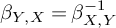
 . However, two half-braidings do not necessarily add up to one braiding, which has to satisfy the hexagon identities for both variables at once. In our case they do add up to a braiding, because they satisfy the additional condition
$\beta _{Y,X}=\beta _{X,Y}^{-1}$
 .
Lemma 4.4. The functor
$\Psi $
 in (85) extends to a monoidal functor, which restricts to the strict monoidal functors
$\Psi _L$
 and
$\Psi _R$
 , if and only if
$\Psi _L, \Psi _R$
 form a symmetric pair of monoidal functors.
Proof. Suppose that
$\Psi $
 extends to a monoidal functor. Then there exists a natural isomorphism

for any objects
$X_1,X_2\in \mathcal {C}$
 and
$Y_1, Y_2\in \mathcal {D}$
 . Note that
$\Psi (\mathbb {1}, \mathbb {1})=\Psi _L(\mathbb {1})\circ _{\mathcal {E}} \Psi _R(\mathbb {1})=\mathbb {1}\circ _{\mathcal {E}} \mathbb {1}=\mathbb {1}$
 holds on the nose, so
$\eta $
 is the only coherence morphism that can be non-trivial.
By definition, the object on the l.h.s. of (89) is equal to

while the object on the r.h.s. is equal to

hence
$\eta _{(X_1,Y_1),(X_2,Y_2)}$
 in (89) is completely determined by the natural isomorphism

where
$\zeta _{X_2, Y_1}:=\eta _{(\mathbb {1},Y_1),(X_2,\mathbb {1})}$
 . Note that we have swapped the order of
$X_2$
 and
$Y_1$
 in the subscript of
$\zeta $
 , which conforms to the notation of a braiding.
Let
$X_1,X_2,X_3\in \mathcal {C}$
 and
$Y_1,Y_2,Y_3\in \mathcal {D}$
 . The usual coherence condition for
$\eta $
 is

where we have suppressed several identity morphisms again. By the same arguments as above, we obtain the corresponding coherence condition for
$\zeta $
 :

Note that the coherence conditions in (93) and (94) are equivalent.
The hexagon identities for
$\zeta $
 are obtained from (94) as special cases, by putting
$Y_2=\mathbb {1}$
 and
$X_2=\mathbb {1}$
 , respectively. This proves that
$\Psi _L, \Psi _R$
 is a symmetric pair of monoidal functors.
Conversely, suppose that
$\Psi _L, \Psi _R$
 is a symmetric pair of monoidal functors with braiding
$\zeta $
 . Thanks to the interchange law for morphisms in a monoidal category, we have

as can be seen from the corresponding commutative diagram:

Multiplying both sides in (95) on the right by
$\zeta _{X_3, Y_1}$
 and using the hexagon identities yields (94), which implies that
$\eta $
 satisfies (93). This proves that
$\Psi $
 extends to a monoidal functor.
The following corollary shows that our choice to define
$\Psi $
 as
$\Psi _L\circ _{\mathcal {E}} \Psi _R$
 , instead of
$\Psi _R\circ _{\mathcal {E}} \Psi _L$
 , is not essential if the pair of monoidal functors
$\Psi _L, \Psi _R$
 is symmetric. The proof uses similar arguments as the proof of Lemma 4.4 and is straightforward, so we leave the details to the reader.
Corollary 4.5. Suppose that
$\Psi _L, \Psi _R$
 is a symmetric pair of monoidal functors. Then
$\Psi _L\circ _{\mathcal {E}} \Psi _R$
 and
$\Psi _R\circ _{\mathcal {E}} \Psi _L$
 are two naturally isomorphic monoidal functors.
Remark 4.6. The functor
$\Psi $
 in Lemma 4.4 is a strict monoidal functor if and only if the braiding
$\zeta $
 is trivial.
4.1.2 Definition of
$\Psi _{k,n-k}$
and main theorem

As in Section 4.1.1, we first define two strict monoidal
$\mathbb {k}$
 -linear functors

and then define

by

for any objects
$X\in \widehat {\mathscr {BS}}^{\mathrm {ext}}_k, Y\in \widehat {\mathscr {BS}}^{\mathrm {ext}}_{n-k}$
 and any morphisms
$f\in \widehat {\mathscr {BS}}^{\mathrm {ext}}_k, g\in \widehat {\mathscr {BS}}^{\mathrm {ext}}_{n-k}$
 . We have omitted the symbol for the monoidal product in
$K^b(\widehat {\mathscr {S}}^{\mathrm {ext}}_n)$
 . To avoid clutter in certain diagrams of the definition below, we have reduced the number of labels. When there are several strands of the same colour, we often label just one of them. The labels of the others are understood to be the same.
On objects
On the generating objects,
$\Psi _L$
 and
$\Psi _R$
 are defined by

On morphisms
-
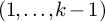
• If $D_{1,\dotsc ,k-1}$
is a morphism of
$\widehat {\mathscr {BS}}^{\mathrm {ext}}_k$
in colours
$(1,\dotsc ,k-1)$
, then $$\begin{align*}\Psi_L(D_{1,\dotsc ,k-1}):=D_{1,\dotsc ,k-1},\end{align*}$$
-
• If $D^{\prime }_{1,\dotsc ,k-1}$
is a morphism of
$\widehat {\mathscr {BS}}^{\mathrm {ext}}_{n-k}$
in colours
$(1,\dotsc ,n-k-1)$
, then $$\begin{align*}\Psi_R(D^{\prime}_{1,\dotsc ,n-k-1}):=D^{\prime}_{k+1,\dotsc ,n-1},\end{align*}$$




On other morphisms,
$\Psi _L$
 and
$\Psi _R$
 are defined as follows.

$\bullet $
 On oriented generators:

$\bullet $
 On generators including strands with distant colours:

for
$1<\color {orange}{i}<k-1$
 and
$1<\color {mygreen}{j}<n-k-1$
 .
$\bullet $
 On generators including strands with adjacent colours:

for
$i,j\neq 0,1$
 , while

and

for
$k\geq 2$
 .

The inner labels in the last line are
${\color {orange}n-1}$
 and
${\color {CadetBlue}[n-2,k-1]}$
 (left) and
${\color {orange}k-1}$
 and
${\color {NavyBlue}[-1,k-2]}$
 (right). This ends the definition of
$\Psi _L$
 and
$\Psi _R$
 .
Lemma 4.7. For any domain X and codomain Y of a generating morphism in
$\widehat {\mathscr {BS}}^{\mathrm {ext}}_k$
 of degree t, we have

Similarly, for any domain Z and codomain W of a generating morphism in
$\widehat {\mathscr {BS}}^{\mathrm {ext}}_{n-k}$
 of degree t, we have

Moreover, all those morphism spaces are one-dimensional.
Proof. The proof is immediate except for two cases in
$\Psi _L$
 and two cases in
$\Psi _R$
 :
-
• a crossing in $\widehat {\mathscr {S}}^{\mathrm {ext}}_k$
involving an oriented strand and unoriented strands labelled
$0$
and
$k-1$
, respectively in
$\widehat {\mathscr {S}}^{\mathrm {ext}}_{n-k}$
with labels
$0$
and
$n-k-1$
; -
• a six-valent vertex in $\widehat {\mathscr {S}}^{\mathrm {ext}}_k$
involving strands labelled
$0$
and
$k-1$
, respectively in
$\widehat {\mathscr {S}}^{\mathrm {ext}}_{n-k}$
with labels
$0$
and
$n-k-1$
.


We only prove the second part of each case, the first being similar.
For a crossing in
${\widehat {\mathscr {S}}}^{\mathrm {ext}}_{n-k}$
 involving an oriented strand and unoriented strands labelled
$0$
 and
$n-k-1$
 we compute

For a six-valent vertex in
${\widehat {\mathscr {S}}}^{\mathrm {ext}}_{n-k}$
 involving strands labelled
$0$
 and
$n-k-1$
 we compute

4.2 Proof of the main theorem
Lemma 4.8. The
$\mathbb {R}$
 -linear, strict monoidal functors
$\Psi _L$
 and
$\Psi _R$
 from Section 4.1.2
-
a) are well-defined;
-
b) form a symmetric pair.
Theorem 4.9. The symmetric pair
$\Psi _L, \Psi _R$
 gives rise to an
$\mathbb {R}$
 -linear, monoidal functor

Proof. By Lemma 4.4 and Lemma 4.8, the
$\mathbb {R}$
 -linear functor in (97)

extends to a monoidal functor, which in turn gives rise to an
$\mathbb {R}$
 -linear, monoidal functor

as explained in Section 4.1.1.
It remains to prove Lemma 4.8, which will be done in Section 4.2.1 and Section 4.2.3.
4.2.1 Well-definedness
The proofs that
$\Psi _L$
 and
$\Psi _R$
 preserve all diagrammatic relations are very similar, so we only prove that
$\Psi _L$
 is well-defined. Because of the two cases in (37), the proof that
$\Psi _L$
 is well-defined contains four cases:
$1=k=n-1$
 ,
$1=k<n-1$
 ,
$2=k<n$
 and
$2<k<n$
 . However, the first two cases are proved in the same way as the corresponding part in the fourth case. The third case is also almost the same as the corresponding part of the fourth case, except for the proof that
$\Psi _L$
 preserves (37), which we therefore prove separately at the end of this subsection.
Suppose that
$k> 2$
 . Since
$\Psi _L$
 is the identity on diagrams only involving colours different from
$0$
 and
$k-1$
 it preserves the relations involving only those diagrams.
-
(a1) Relations (26) to (29) for $i=0$
follow by isotopy and similar arguments as in the first bullet point in the proof of [Reference Mackaay, Miemietz and VazMMV, Theorem 5.4]. -
(a2) Relations (30) to (33) for $i=0$
or
$k=0$
are verified using the relations in (68) and the usual Soergel calculus. -
(a3) Relations (34) to (37) for $\{i,j\}=\{0,1\}$
are checked using similar arguments as in the third bullet point in the proof of [Reference Mackaay, Miemietz and VazMMV, Theorem 5.4]. -
(a4) Relations (34) to (37) for $\{i,j\}=\{0,k-1\}$
are more involved and we give a sample computation for relation (35), with the proof of the other relations being similar. We have where the missing labels in the inner part of the diagram are ${\color {PineGreen}n-1}$
and
${\color {RawSienna}[n-2,k-1]}$
. Using (59) twice on the strands labelled
${\color {RawSienna}[n-2,k-1]}$
on the first term, and (68) on the second gives -
(a5) Relation (38) for one of the labels being $0$
follows easily. -
(a6) The relevant cases for relation (39) are $\{i,j\}=\{0,1\}$
,
$\{i,j\}=\{0,k-1\}$
or
$k=0$
and all are straightforward. -
(a7) The relevant cases for relation (40) are $(i,j,k)=(0,1,2)$
,
$(i,j,k)=(k-1,0,1)$
and
$(i,j,k)=(k-2,k-1,0)$
. Using arguments similar to the seventh bullet point in the proof of [Reference Mackaay, Miemietz and VazMMV, Theorem 5.4] one verifies the first case. We provide the proof of the second and the third is similar.Applying $\Psi _L$
to the left-hand side of (40) yields (the unlabelled strands of the diagrams on the right-hand side have labels
${\color {RawSienna}[n-2,k-1]}$
,
${\color {orange}k-1}$
) A similar procedure gives
Relation (40) for labels $(k-1,0,1)$
implies that they are equal. -
(a8) Relations (41) and (42) are an easy consequence of (57) and (59).
-
(a9) Relation (43) is immediate if $0\notin \{i-1,i,j-1,j\}$
. The remaining cases can be proved using relations (74), (81) and (83). -
(a10) Checking relation (44) uses only Lemma 3.5 and relations (71) and (63) unless $(i-1,i)=(k-1,0)$
. The remaining cases use (77) and (63). Relation (45) is verified using Lemma 3.5 and relations (63) and (80). For (46) the only case that is not immediate is when
$i=0$
. In this case, -
(a11) For relations (47) we need to consider the cases $i-1=0$
,
$i=0$
and
$i+1=0$
. The first case uses (68) and (57).In the remaining cases, we prove the first relation, the second one being similar.
For $i=0$
we compute For the case $i+1=0$
we use the hom & dot trick. We have that (98)define morphisms in
$$\begin{align*}\mathrm{hom}_{K^b({\widehat{\mathscr{S}}}^{\mathrm{ext}}_n)}&\left({\mathrm{T}}_{[n-1,k]}^{-1} {\mathrm{B}}_0 {\mathrm{T}}_{[n\!-\!1,k]} \mathrm{B}_{k-1} {\mathrm{T}}_{[n-1,k]}^{-1} \mathrm{B}_0 {\mathrm{T}}_{[n-1,k]}, \mathrm{B}_\rho {\mathrm{T}}_{[n-1,k]}\right.\\&\qquad \left.{\mathrm{B}}_{k-2}{\mathrm{B}}_{k-1}{\mathrm{B}}_{k-2}{\mathrm{T}}_{[n-1,k]}^{-1}{\mathrm{B}}_{\rho}^{-1}\right). \end{align*}$$
This morphism space is one-dimensional, as can be seen as follows. By (75) (with $a=k$
and
$b=0$
) and (68), we have
${\mathrm {T}}_{[n-1,k]}^{-1} {\mathrm {B}}_0 {\mathrm {T}}_{[n\!-\!1,k]}\simeq {\mathrm {T}}_{[n,k+1]} {\mathrm {B}}_{k}{\mathrm {T}}_{[n,k+1]}^{-1}$
and
${\mathrm {T}}_{[n,k+1]} {\mathrm {B}}_{k-1}\simeq {\mathrm {B}}_{k-1} {\mathrm {T}}_{[n,k+1]}$
. This implies that the domain is homotopy equivalent to
${\mathrm {T}}_{[n,k+1]} {\mathrm {B}}_k\mathrm {B}_{k-1} \mathrm {B}_k {\mathrm {T}}_{[n,k+1]}^{-1}$
. Commuting
$\mathrm {B}_\rho $
with all factors from left to right shows that the codomain is homotopy equivalent to
${\mathrm {T}}_{[n,k+1]} {\mathrm {B}}_{k-1}{\mathrm {B}}_{k} \mathrm {B}_{k-1} {\mathrm {T}}_{[n,k+1]}^{-1}$
. By adjunction, the above morphism space is therefore isomorphic to
$\mathrm {hom}_{K^b({\widehat {\mathscr {S}}}^{\mathrm {ext}}_n)}\left ( {\mathrm {B}}_k{\mathrm {B}}_{k-1} {\mathrm {B}}_k, {\mathrm {B}}_{k-1}{\mathrm {B}}_{k} {\mathrm {B}}_{k-1}\right )$
. Moreover, we have $$\begin{align*}\mathrm{hom}_{K^b({\widehat{\mathscr{S}}}^{\mathrm{ext}}_n)}\left( {\mathrm{B}}_k{\mathrm{B}}_{k-1} {\mathrm{B}}_k, {\mathrm{B}}_{k-1}{\mathrm{B}}_{k} {\mathrm{B}}_{k-1}\right)\cong \mathrm{hom}_{{\widehat{\mathscr{S}}}^{\mathrm{ext}}_n}\left( {\mathrm{B}}_k{\mathrm{B}}_{k-1} {\mathrm{B}}_k, {\mathrm{B}}_{k-1}{\mathrm{B}}_{k} {\mathrm{B}}_{k-1}\right) \end{align*}$$
and the latter morphism space is one-dimensional (thanks to Soergel’s hom formula in (49)).
We attach a dot to the free end at the top labelled $\color {orange}k-1$
of the diagrams at the right-hand sides of (98). For the left diagram in (98), use (34) to get rid of the 6-valent vertex and obtain two terms which can be further simplified by relations (80), (45), (63) and (77). For the right diagram in (98), first use (80), (45), (63) and (68) to slide the dot closer to the 6-valent vertex, then proceed as in the previous case. In the end, we see that both diagrams in (98) become equal to


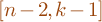
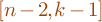








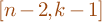












This completes the proof that
$\Psi _L$
 is well-defined for
$k\ne 2$
 .
Now, let
$k=2$
 . As already mentioned, it only remains to check (37) in this case. We have

Now, with
$0$
 and
$1$
 switched,

where in the second equality we used (an easy consequence of [Reference Mackaay, Miemietz and VazMMV, Lemma 4.6])

and in the third equality we used (37) twice, one involving labels
$\color {blue}1$
 and
$\color {violet}0$
 and the other involving colours
$\color {violet}0$
 and
$\color {orange}n-1$
 .
This completes the proof of the last case.
4.2.2 Definition of
$\zeta $

We will first show that for every pair of objects
$X\in \widehat {\mathscr {BS}}^{\mathrm {ext}}_k, Y\in \widehat {\mathscr {BS}}^{\mathrm {ext}}_{n-k}$
 , there is an isomorphism in
$K^b({\widehat {\mathscr {S}}}^{\mathrm {ext}}_n)$


and that these isomorphisms satisfy the hexagon identities from Definition 4.2. After that, we will show that
$\zeta $
 is natural in X and Y.
We define
$\zeta _{X,Y}$
 for pairs of generating objects
$X\in \{{\mathrm {B}}_i,{\mathrm {B}}_\rho \}\subset \mathrm {Ob}(\widehat {\mathscr {BS}}^{\mathrm {ext}}_k)$
 and
$Y\in \{{\mathrm {B}}_i,{\mathrm {B}}_\rho \}\subset \mathrm {Ob}(\widehat {\mathscr {BS}}^{\mathrm {ext}}_{n-k})$
 and extend the definition recursively to pairs of monoidal products of generating objects (corresponding to Bott-Samelson bimodules) by the hexagon identities. Concretely, we put

for any objects
$X_1,X_2\in \widehat {\mathscr {BS}}^{\mathrm {ext}}_k$
 and
$Y_1,Y_2\in \widehat {\mathscr {BS}}^{\mathrm {ext}}_{n-k}$
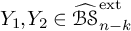 . Alternatively, we could have put

but the expressions in (99) and (100) are equal because
$\zeta _{X_1,Y_1}\cdot \zeta _{X_2,Y_2}= \zeta _{X_2,Y_2}\cdot \zeta _{X_1,Y_1}$
 thanks to the interchange law, see (95). In particular, the isomorphisms
$\zeta _{X,Y}$
 satisfy the hexagon identities by definition.
After this explanation, it remains to define
$\zeta _{X,Y}$
 for pairs of generating objects.
In all cases below,
$\zeta _{X,Y}$
 is obtained by composing invertible morphisms in
$K^b({\widehat {\mathscr {S}}}^{\mathrm {ext}}_n)$
 . To see this, one notes that all diagrams appearing are isotopic to a diagram where at each height there is either a merger or a splitter, a four-valent vertex (a crossing), a six-valent one (all involving at least one oriented strand), or just vertical strands. One checks easily that all of them are invertible (this is implied by the various relations in Section 3.1 and Section 3.2), hence so is their composite. Therefore, we only give the diagrams for
$\zeta _{X,Y}$
 without further explanation.


In
$\zeta _{{\mathrm {B}}_\rho ,{\mathrm {B}}_0}$
 ,
$\color {Salmon}{\mathrm {T}}_{[-1,k\!-\!2]}={\mathrm {T}}_{n-1}{\mathrm {T}}_{0}{\mathrm {T}}_{1}\dotsm {\mathrm {T}}_{k-2}$
 , and in
$\zeta _{{\mathrm {B}}_0,{\mathrm {B}}_0}$
 ,
$\color {WildStrawberry}a=[1,k\!-\!2]$
 and
$\color {Cyan}b=[n\!-\!2,k\!+\!1]$
 .
This completes the definition of
$\zeta $
 .
Remark 4.10. Diagrams for
$\zeta $
 involving inverses of
${\mathrm {B}}_\rho ^{-1}$
 are obtained easily by applying the appropriate adjunctions and taking inverses (if necessary). We have

and similarly for
$\zeta _{{\mathrm {B}}_\rho ^{-1},\mathrm {B}_{\rho }}^{-1}$
 . A rotation of
$\zeta _{\mathrm {B}_\rho ,\mathrm {B}_\rho }$
 by 180 degrees yields
$\zeta _{\mathrm {B}_\rho ^{-1},\mathrm {B}_\rho ^{-1}}$
 .
4.2.3 Naturality of
$\zeta $

To show that
$\zeta $
 is natural, we have to prove commutativity of the diagram

for all objects
$X,W\in \widehat {\mathscr {BS}}^{\mathrm {ext}}_k$
 and
$Y,Z\in \widehat {\mathscr {BS}}^{\mathrm {ext}}_{n-k}$
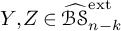 , and all morphisms
$f\in \mathrm {hom}_{\widehat {\mathscr {BS}}^{\mathrm {ext}}_k}(X,W)$
 and
$g\in \mathrm {hom}_{\widehat {\mathscr {BS}}^{\mathrm {ext}}_{n-k}}(Y,Z)$
 . Thanks to the hexagon identities for
$\zeta $
 and the interchange law for morphisms in
$K^b({\widehat {\mathscr {S}}}^{\mathrm {ext}}_n)$
 , it suffices to show commutativity in (101) for pairs
$(f,g)$
 where f is a generating morphism in
$\widehat {\mathscr {BS}}^{\mathrm {ext}}_k$
 and
$g=\mathrm {id}_Y$
 for some generating object
$Y\in \widehat {\mathscr {BS}}^{\mathrm {ext}}_{n-k}$
 , or
$f=\mathrm {id}_X$
 for some generating object
$X\in \widehat {\mathscr {BS}}^{\mathrm {ext}}_k$
 and g is a generating morphism in
$\widehat {\mathscr {BS}}^{\mathrm {ext}}_{n-k}$
 . Finally, we note that the proof for pairs of the first type and the proof for pairs of the second type are very similar, so we only give the proof for pairs of the second type below. Concretely, those pairs are
$(\mathrm {id}_X, g)$
 , where
$X\in \{{\mathrm {B}}_\rho , {\mathrm {B}}_0, \ldots , {\mathrm {B}}_{k-1}\}$
 and g is one of the generators in (23), (24) or (25) with labels in
$\{\rho , 0,\ldots , n-k-1\}$
 . The only cases in which commutativity of (101) is not immediate, is when
$X\in \{{\mathrm {B}}_\rho , {\mathrm {B}}_0\}$
 and/or the labels of some strands of g belong to
$\{0, \rho \}$
 .
Note that checking commutativity of (101) always consists of verifying the equality of two diagrams, both belonging to the same morphism space. In all but two cases the dimension of the morphism space in the given degree is one-dimensional (see Lemma 4.11), so we can use the hom & dot trick, explained in Remark 3.7. The remaining two cases are checked directly.
Lemma 4.11. For each generating object X of
$\widehat {\mathscr {BS}}^{\mathrm {ext}}_{k}$
 and each generating morphism
$g\colon Y\to Z$
 in
$\widehat {\mathscr {BS}}^{\mathrm {ext}}_{n-k}$
 , there are objects
$U,V\in \widehat {\mathscr {BS}}^{\mathrm {ext}}_n$
 and an isomorphism

Unless
$X={\mathrm {B}}_0$
 and
$g\colon 1\to {\mathrm {B}}_0$
 is a dot labelled 0 or
$g\colon \mathrm {B}_0\to \mathrm {B}_0\mathrm {B}_0$
 is a trivalent vertex labelled 0, the two morphism spaces in (102) are one-dimensional by Soergel’s hom formula in (102) are one-dimensional by Soergel’s hom formula in (49).
Proof. We first note that by invertibility of
$\zeta _{X,Z}$
 we have
$\Psi _R(Z)\Psi _L(X)\cong \Psi _L(X)\Psi _R(Z)$
 and we need compute
$\hom _{K^b({\widehat {\mathscr {S}}}^{\mathrm {ext}}_n)}(\Psi _L(X)\Psi _R(Y),\Psi _L(X)\Psi _R(Z))$
 . For invertible X, the claim follows from Lemma 4.7 and therefore we have to consider only the cases
$X={\mathrm {B}}_i$
 . The case of
$i>0$
 is an easy computation in the lines of the proof of Lemma 4.7. For
$i=0$
 we proceed case-by-case.
-
• For
, $$ \begin{align*} \hom_{K^b({\widehat{\mathscr{S}}}^{\mathrm{ext}}_n)}&(\Psi_L({\mathrm{B}}_0), \Psi_L({\mathrm{B}}_0) \Psi_R({\mathrm{B}}_0)\langle 1\rangle) \\&= \hom_{K^b({\widehat{\mathscr{S}}}^{\mathrm{ext}}_n)}({\mathrm{T}}_{[n-1,k]}^{-1}{\mathrm{B}}_0{\mathrm{T}}_{[n-1,k]},{\mathrm{T}}_{[n-1,k]}^{-1}{\mathrm{B}}_0{\mathrm{T}}_{[n-1,k]}{\mathrm{T}}_{[0,k-1]}\\&\quad\ {\mathrm{B}}_k{\mathrm{T}}_{[0,k-1]}^{-1}\langle 1\rangle) \\&\cong \hom_{K^b({\widehat{\mathscr{S}}}^{\mathrm{ext}}_n)}(\mathbb{1},{\mathrm{B}}_0{\mathrm{T}}_{[n-1,k]}{\mathrm{T}}_{[0,k-1]}{\mathrm{B}}_k{\mathrm{T}}_{[0,k-1]}^{-1}{\mathrm{T}}_{[n-1,k]}^{-1}{\mathrm{B}}_0\langle 1\rangle) \\ &\cong \hom_{K^b({\widehat{\mathscr{S}}}^{\mathrm{ext}}_n)}(\mathbb{1},{\mathrm{B}}_0{\mathrm{T}}_{[n-1,k]}{\mathrm{T}}_{[1,k]}^{-1}{\mathrm{B}}_0{\mathrm{T}}_{[1,k]}{\mathrm{T}}_{[n-1,k]}^{-1}{\mathrm{B}}_0\langle 1\rangle) \\ &\cong \hom_{K^b({\widehat{\mathscr{S}}}^{\mathrm{ext}}_n)}(\mathbb{1},{\mathrm{B}}_0{\mathrm{T}}_{[1,k-1]}^{-1}{\mathrm{T}}_{[n-1,k+1]}{\mathrm{B}}_0{\mathrm{T}}_{[n-1,k+1]}^{-1}{\mathrm{T}}_{[1,k-1]}{\mathrm{B}}_0\langle 1\rangle) \\ &\cong \hom_{K^b({\widehat{\mathscr{S}}}^{\mathrm{ext}}_n)}(\mathbb{1},{\mathrm{B}}_0{\mathrm{T}}_1^{-1}{\mathrm{T}}_0{\mathrm{B}}_1{\mathrm{T}}_0^{-1}{\mathrm{T}}_1{\mathrm{B}}_0\langle 1\rangle) \\ &\cong \hom_{K^b({\widehat{\mathscr{S}}}^{\mathrm{ext}}_n)}(\mathbb{1},{\mathrm{B}}_1{\mathrm{B}}_1{\mathrm{B}}_1\langle 1\rangle) \cong \hom_{K^b({\widehat{\mathscr{S}}}^{\mathrm{ext}}_n)}({\mathrm{B}}_1,{\mathrm{B}}_1{\mathrm{B}}_1\langle 1\rangle) \\ &\cong \hom_{{\widehat{\mathscr{S}}}^{\mathrm{ext}}_n}({\mathrm{B}}_1,{\mathrm{B}}_1{\mathrm{B}}_1\langle 1\rangle) \cong \mathbb{R}^3. \end{align*} $$
-
• For
, $$ \begin{align*} & \hom_{K^b({\widehat{\mathscr{S}}}^{\mathrm{ext}}_n)}(\Psi_L({\mathrm{B}}_0)\Psi_R({\mathrm{B}}_0), \Psi_L({\mathrm{B}}_0)\Psi_R({\mathrm{B}}_0{\mathrm{B}}_0)\langle -1\rangle) \\ & \qquad\qquad = \hom_{K^b({\widehat{\mathscr{S}}}^{\mathrm{ext}}_n)}({\mathrm{T}}_{[n-1,k]}^{-1}{\mathrm{B}}_0{\mathrm{T}}_{[n-1,k]}{\mathrm{T}}_{[0,k-1]}{\mathrm{B}}_k{\mathrm{T}}_{[0,k-1]}^{-1} , \\ & \qquad\qquad {\mathrm{T}}_{[n-1,k]}^{-1}{\mathrm{B}}_0{\mathrm{T}}_{[n-1,k]}{\mathrm{T}}_{[0,k-1]}{\mathrm{B}}_k{\mathrm{T}}_{[0,k-1]}^{-1}{\mathrm{T}}_{[0,k-1]}{\mathrm{B}}_k{\mathrm{T}}_{[0,k-1]}^{-1}\langle -1\rangle ) \\ &\cong \hom_{K^b({\widehat{\mathscr{S}}}^{\mathrm{ext}}_n)}({\mathrm{B}}_0{\mathrm{T}}_{[n-1,k]}{\mathrm{T}}_{[0,k-1]}{\mathrm{B}}_k , {\mathrm{B}}_0{\mathrm{T}}_{[n-1,k]}{\mathrm{T}}_{[0,k-1]}{\mathrm{B}}_k{\mathrm{B}}_k\langle -1\rangle ) \\ &\cong \hom_{K^b({\widehat{\mathscr{S}}}^{\mathrm{ext}}_n)}({\mathrm{B}}_0{\mathrm{B}}_0 , \mathrm{B}_0\mathrm{B}_0\mathrm{B}_0\langle -1\rangle )\\ &\cong \hom_{{\widehat{\mathscr{S}}}^{\mathrm{ext}}_n}({\mathrm{B}}_0{\mathrm{B}}_0 , {\mathrm{B}}_0{\mathrm{B}}_0{\mathrm{B}}_0\langle -1\rangle ) \cong \mathbb{R}^5. \end{align*} $$
The remaining morphism spaces are one-dimensional. This can be checked using the same type of computation as in the two cases above.
-
• For
, $$ \begin{align*}&\mathrm{hom}_{K^b(\widehat{\mathcal{S}}^{\mathrm{ext}}_n)}\bigl(\Psi_L(B_0)\Psi_R(B_0B_j),\Psi_L(B_0)\Psi_R(B_jB_0)\bigr)\\&\quad =\mathrm{hom}_{K^b(\widehat{\mathcal{S}}^{\mathrm{ext}}_n)}\Bigl(T^{-1}_{[n-1,k]}B_0T_{[n-1,k]}T_{[0,k-1]}B_kT^{-1}_{[0,k-1]}B_{j+k},\\&\quad\qquad\qquad T^{-1}_{[n-1,k]}B_0T_{[n-1,k]}B_{k+j}T_{[0,k-1]}B_kT^{-1}_{[0,k-1]}\Bigr)\\&\quad\cong\mathrm{hom}_{\widehat{\mathcal{S}}^{\mathrm{ext}}_n}\bigl(B_{n-1}B_{k-1}B_{j+k-1},B_{n-1}B_{k-1}B_{j+k-1}\bigr)\cong \mathbb{R}.\end{align*} $$
-
• For
, $$ \begin{align*} \hom_{K^b({\widehat{\mathscr{S}}}^{\mathrm{ext}}_n)}&(\Psi_L({\mathrm{B}}_0)\Psi_R({\mathrm{B}}_\rho{\mathrm{B}}_{j-1}), \Psi_L({\mathrm{B}}_0)\Psi_R({\mathrm{B}}_j{\mathrm{B}}_\rho))\\ & = \hom_{K^b({\widehat{\mathscr{S}}}^{\mathrm{ext}}_n)}({\mathrm{T}}_{[n-1,k]}^{-1}{\mathrm{B}}_0{\mathrm{T}}_{[n-1,k]}{\mathrm{T}}_{[1,k]}^{-1}{\mathrm{B}}_\rho{\mathrm{B}}_{j+k-1} , {\mathrm{T}}_{[n-1,k]}^{-1}{\mathrm{B}}_0{\mathrm{T}}_{[n-1,k]}\\ & {\mathrm{B}}_{j+k}{\mathrm{T}}_{[1,k]}^{-1}{\mathrm{B}}_\rho )\\ &\cong \hom_{{\widehat{\mathscr{S}}}^{\mathrm{ext}}_n}({\mathrm{B}}_0{\mathrm{B}}_{j+k-1} , {\mathrm{B}}_0{\mathrm{B}}_{j+k-1} ) \cong \mathbb{R}. \end{align*} $$
-
• For
, $$ \begin{align*} \hom_{K^b({\widehat{\mathscr{S}}}^{\mathrm{ext}}_n)}&(\Psi_L({\mathrm{B}}_0)\Psi_R({\mathrm{B}}_\rho{\mathrm{B}}_0) , \Psi_L({\mathrm{B}}_0)\Psi_R({\mathrm{B}}_1{\mathrm{B}}_\rho)) \\ & = \hom_{K^b({\widehat{\mathscr{S}}}^{\mathrm{ext}}_n)}({\mathrm{T}}_{[n-1,k]}^{-1}{\mathrm{B}}_0{\mathrm{T}}_{[n-1,k]}{\mathrm{T}}_{[1,k]}^{-1}{\mathrm{B}}_\rho {\mathrm{T}}_{[0,k-1]}{\mathrm{B}}_k{\mathrm{T}}_{[n-1,k]}^{-1} , {\mathrm{T}}_{[n-1,k]}^{-1}\\&\qquad{\mathrm{B}}_0{\mathrm{T}}_{[n-1,k]}{\mathrm{B}}_{1+k}{\mathrm{T}}_{[1,k]}^{-1}{\mathrm{B}}_\rho ) \\ &\cong \hom_{{\widehat{\mathscr{S}}}^{\mathrm{ext}}_n}({\mathrm{B}}_0{\mathrm{B}}_{k} , {\mathrm{B}}_0{\mathrm{B}}_{k} ) \cong \mathbb{R}. \end{align*} $$
-
• For
, $$ \begin{align*} \hom_{K^b({\widehat{\mathscr{S}}}^{\mathrm{ext}}_n)}&(\Psi_L({\mathrm{B}}_0)\Psi_R({\mathrm{B}}_\rho{\mathrm{B}}_{n-k-1}), \Psi_L({\mathrm{B}}_0)\Psi_R({\mathrm{B}}_0{\mathrm{B}}_\rho)) \\ & = \hom_{K^b({\widehat{\mathscr{S}}}^{\mathrm{ext}}_n)}({\mathrm{T}}_{[n-1,k]}^{-1}{\mathrm{B}}_0{\mathrm{T}}_{[n-1,k]} {\mathrm{T}}_{[1,k]}^{-1}{\mathrm{B}}_\rho {\mathrm{B}}_{n-1} , {\mathrm{T}}_{[n-1,k]}^{-1}\\&\qquad{\mathrm{B}}_0{\mathrm{T}}_{[n-1,k]} {\mathrm{T}}_{[0,k-1]}{\mathrm{B}}_{k}{\mathrm{T}}_{[0,k-1]}^{-1}{\mathrm{T}}_{[1,k]}^{-1}{\mathrm{B}}_\rho ) \\ &\cong \hom_{{\widehat{\mathscr{S}}}^{\mathrm{ext}}_n}({\mathrm{B}}_{n-1}{\mathrm{B}}_{k-1} , {\mathrm{B}}_{n-1}{\mathrm{B}}_{k-1} ) \cong \mathbb{R}. \end{align*} $$
-
• For
, $$ \begin{align*} \hom_{K^b({\widehat{\mathscr{S}}}^{\mathrm{ext}}_n)}&(\Psi_L({\mathrm{B}}_0)\Psi_R({\mathrm{B}}_1{\mathrm{B}}_0{\mathrm{B}}_1), \Psi_L({\mathrm{B}}_0)\Psi_R({\mathrm{B}}_0{\mathrm{B}}_1{\mathrm{B}}_0)) \\ & = \hom_{K^b({\widehat{\mathscr{S}}}^{\mathrm{ext}}_n)}({\mathrm{T}}_{[n-1,k]}^{-1}{\mathrm{B}}_0{\mathrm{T}}_{[n-1,k]} {\mathrm{B}}_{k+1}{\mathrm{T}}_{[0,k-1]}{\mathrm{B}}_{k}{\mathrm{T}}_{[0,k-1]}^{-1}{\mathrm{B}}_{k+1} , \\ &\qquad {\mathrm{T}}_{[n-1,k]}^{-1}{\mathrm{B}}_0{\mathrm{T}}_{[n-1,k]} {\mathrm{T}}_{[0,k-1]}{\mathrm{B}}_{k}{\mathrm{T}}_{[0,k-1]}^{-1}{\mathrm{B}}_{k+1}{\mathrm{T}}_{[0,k-1]}{\mathrm{B}}_{k}{\mathrm{T}}_{[0,k-1]}^{-1} ) \\ &\cong \hom_{{\widehat{\mathscr{S}}}^{\mathrm{ext}}_n}({\mathrm{B}}_{n-1}{\mathrm{B}}_k{\mathrm{B}}_{k-1}{\mathrm{B}}_k , {\mathrm{B}}_{n-1}{\mathrm{B}}_{k-1}{\mathrm{B}}_k{\mathrm{B}}_{k-1} ) \cong \mathbb{R}. \end{align*} $$
-
• For
, $$ \begin{align*} \hom_{K^b({\widehat{\mathscr{S}}}^{\mathrm{ext}}_n)}&(\Psi_L({\mathrm{B}}_0)\Psi_R({\mathrm{B}}_{n-k-1}{\mathrm{B}}_0{\mathrm{B}}_{n-k-1}), \Psi_L({\mathrm{B}}_0)\Psi_R({\mathrm{B}}_0{\mathrm{B}}_{n-k-1}{\mathrm{B}}_0)) \\ & = \hom_{K^b({\widehat{\mathscr{S}}}^{\mathrm{ext}}_n)}({\mathrm{T}}_{[n-1,k]}^{-1}{\mathrm{B}}_0{\mathrm{T}}_{[n-1,k]} {\mathrm{B}}_{n-1}{\mathrm{T}}_{[0,k-1]}{\mathrm{B}}_{k}{\mathrm{T}}_{[0,k-1]}^{-1}{\mathrm{B}}_{n-1} , \\ &\qquad {\mathrm{T}}_{[n-1,k]}^{-1}{\mathrm{B}}_0{\mathrm{T}}_{[n-1,k]} {\mathrm{T}}_{[0,k-1]}{\mathrm{B}}_{k}{\mathrm{T}}_{[0,k-1]}^{-1}{\mathrm{B}}_{n-k-1}{\mathrm{T}}_{[0,k-1]}{\mathrm{B}}_{k}{\mathrm{T}}_{[0,k-1]}^{-1} ) \\ &\cong \hom_{{\widehat{\mathscr{S}}}^{\mathrm{ext}}_n}({\mathrm{B}}_{k+1}{\mathrm{B}}_{k-1}{\mathrm{B}}_k{\mathrm{B}}_{k-1} , {\mathrm{B}}_{k+1}{\mathrm{B}}_k{\mathrm{B}}_{k-1}{\mathrm{B}}_k ) \cong \mathbb{R}. \end{align*} $$


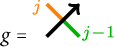


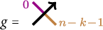


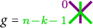

Before checking commutativity of (101), we need a technical lemma. In the following, a rectangular region of a diagram decorated with a
$\zeta _{X,Y}$
 will be called a box.
Lemma 4.12. The following relations involving boxes and dots hold in
$\mathsf {{K}}^b({\widehat {\mathscr {S}}}^{\mathrm {ext}}_n)$
 :


and analogous relations with the dot being attached to any other free end.
Proof. Relations (103) and (104) are immediate.
Proof of (105). By (59) the l.h.s. can be written as

Introducing the diagram of
$\zeta _{{\mathrm {B}}_\rho ,{\mathrm {B}}_0}$
 from Section 4.2.3 and computing yields

In the equality above, we have used (80) to simplify the only 6-valent vertex appearing (involving labels k and
$k-1$
 , followed by (68) and (45) to slide the dot to the top of the diagram, (61) to simplify the digons involving strands labelled k and
$k-1$
 that were created by (80), and finally (57) to simplify the loop labelled
$k-1$
 (created by applying (61)).
Applying (65) to the strands labelled
$[n\!-\!2,k]$
 and
$[0,k\!-\!2]$
 gives

which is the r.h.s. of (105).
Proof of (106). We introduce the diagram for
$\zeta _{{\mathrm {B}}_0,{\mathrm {B}}_0}$
 in the left-hand side of (106) and compute


The proof of the analogous relations with the dot being attached at any other free end is similar.
Now we are ready to prove the naturality of
$\zeta $
 .
-
(N1) For $X={\mathrm {B}}_{\rho }$
and
commutativity of (101) follows from (105). -
(N2) For $X=B_\rho $
and
, we have to check (107)We use the hom & dot trick and attach dots to the upper endpoints labelled $\color {Violet}k$
on both diagrams and then use the analogue of (105) with the dot on the top end to pass the dots past the boxes with
$\zeta _{{\mathrm {B}}_\rho ,{\mathrm {B}}_0}$
.The right-hand side of (107) gives
while for the left-hand side we have
which equals the right-hand side by (26).
-
(N3) For the cases $X={\mathrm {B}}_\rho $
,
and
$X={\mathrm {B}}_\rho $
,
we have to check (108)and
(109)respectively.
Both equalities can be checked to hold by using the hom & dot trick: attach a dot to the top endpoints labelled $\color {orange}k+1$
and use (103). -
(N4) For $X=B_\rho $
and
we have to check (110)We use the hom & dot trick and attach a dot on the top endpoints labelled $\color {blue}k+1$
of both sides of (110). The left-hand side is simplified using (103) (with
$j=1$
), followed by (59) on the two strands labelled
$[1,k]$
and (63). On the right-hand side, we use (45), followed by (105) and then (63) on the two strands labelled
$[1,k]$
and (63). The resulting diagram, in both cases, is -
(N5) For $X=B_\rho $
and
we have to check (111)We use the hom & dot trick and attach a dot on the top endpoints labelled $\color {Violet}k$
of both sides of (111). The left-hand side is simplified using (105), followed by (45), (80), (63) and (57). On the right-hand side, we use (45) followed by (80), (63) and (103). The resulting diagram, in both cases, is -
(N6) The cases $X=B_\rho $
,
and
$X=B_\rho $
,
are very similar. We only prove the first case here. We have to check (112)We use the hom & dot trick and attach a dot on all endpoints labelled $\color {Violet}k$
and
$\color {blue}k+1$
of both sides of (112). On the right-hand side, we use (105), along with (103), to pull all dots from the bottom to the top. The resulting diagram is On the left-hand side we first use (34) on the six-valent vertex, which results in two terms with dots on the bottom ends. We then use (105) several times and (103) on the resulting diagrams, along with (68) to pull all dots and barbells to to left top. This results in
which equals the right-hand side since
-
(N7) For $X={\mathrm {B}}_0$
and
we cannot use the hom & dot trick (see Lemma 4.11). Commutativity of (101) in this case follows from (106) rotated 180 degrees. -
(N8) For $X=B_0$
and
, we cannot use the hom & dot trick (see Lemma 4.11). We have to check (113)We introduce the diagram for $\zeta _{{\mathrm {B}}_0,{\mathrm {B}}_0}$
in the left-hand side of (113) and compute which equals the right-hand side of (113) by (68), (32) and (82).
-
(N9) For the cases $X={\mathrm {B}}_0$
,
and
$X={\mathrm {B}}_0$
,
we have to check (114)and
(115)respectively.
Both equalities can be checked to hold by using the hom & dot trick: attach a dot to the top endpoints labelled $\color {orange}k+1$
and use (104). -
(N10) For $X=B_0$
and
we have to check (116)We use the hom & dot trick and attach a dot on the top endpoint labelled $\color {blue}k+1$
of both sides of (116). The left-hand side is simplified using (104) (with
$j=k+1$
), followed by (45), (59) on the two strands labelled
$[1,k]$
, and (63). On the right-hand side, we use (45), (59) on the two strands labelled
$[1,k]$
, (63), and finally (106) to pull the dot across the box
$\zeta _{{\mathrm {B}}_0,{\mathrm {B}}_0}$
to the bottom right.The resulting diagram, in both cases, is
-
(N11) For $X=B_0$
and
we have to check (117)We use the hom & dot trick and attach a dot on the top endpoints labelled $\color {Violet}k$
of both sides of (117). The left-hand side is simplified using (106), followed by (45), (80), (63) and (57). On the right-hand side, we use (45) followed by (80), (63) and (104). The resulting diagram, in both cases, is -
(N12) The cases $X=B_0$
,
and and
$X=B_\rho $
,
are very similar. We only prove the first case here. We have to check (118)We use the hom & dot trick. At the top of both diagrams we attach a dot at the endpoints labelled $\color {violet}0$
and
$\color {Violet}k$
. At the bottom we attach dots to the endpoints labelled
$\color {violet}0$
,
$\color {Violet}k$
and the leftmost endpoint labelled
${\color {blue}k+1}$
.On the resulting diagram at the left-hand side, we use (106) twice and (104) to pull all dots to the bottom. Using (59) and (68) we obtain
(119)On the right-hand side, we use (a variant of) (104) to pull the dots labelled $\color {violet}0$
close to the box
$\zeta _{{\mathrm {B}}_0,{\mathrm {B}}_0}$
and use (59) to obtain (120)Finally, applying (106) to slide the dot labelled $\color {purple}k$
up through the box, using (68) to slide the dot labelled
$\color {blue}k\!+\!1$
through the strand labelled
$\color {purple}[0,k\!-\!1]$
, and using (59) on the strands labelled
$\color {purple}[0,k\!-\!1]$
with endpoints at the bottom gives (119).


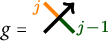


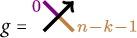


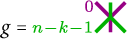


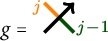


This ends the proof of the naturality of
$\zeta $
 .
Remark 4.13. Naturality for morphisms involving
${\mathrm {B}}_\rho ^{-1}$
 is easy to check by applying adjunctions (see Remark 4.10). For example, for
$X={\mathrm {B}}_\rho $
 and
 we have

4.2.4 A conjecture regarding faithfulness
Note that the functor
$\Psi _{k,n-k} $
 , as defined above, is not faithful.
Lemma 4.14. Recalling (48), we have
$\Psi _{k,n-k}\big (\fbox{y} ,\varnothing \big ) = \fbox{y} = \Psi _{k,n-k}\big (\varnothing ,\fbox{y} \big )$
 .
Proof. An easy computation using the definition of
$\Psi _{k,n-k}$
 and Lemma 3.6.
Define
${\widehat {\mathscr {S}}}^{\mathrm {ext}}_k \boxtimes _y \widehat {\mathscr {S}}^{\mathrm {ext}}_{n-k}$
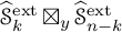 as the usual box tensor product, but with the morphism spaces tensored over the polynomial algebra
$\mathbb {R}[\fbox{y} ]$
 .
Conjecture 4.15. The functor
$\Psi _{k,n-k}$
 descends to a faithful functor
${\widehat {\mathscr {S}}}^{\mathrm {ext}}_{k}\boxtimes _y {\widehat {\mathscr {S}}}^{\mathrm {ext}}_{n-k}\to K^b({\widehat {\mathscr {S}}}^{\mathrm {ext}}_{n})$
 .
5 Parabolic induction: an example
5.1 The decategorified story
In this section, we will work out an explicit example of an induced triangulated birepresentation
$\mathbf {W}$
 of
${\widehat {\mathscr {S}}}^{\mathrm {ext}}_2$
 and its wide finitary cover
$\mathbf {U}$
 . Below, we will start with the decategorified story, before we move on to the categorification, after a general intermezzo on completions of additive categories. The categorified story is divided into two parts: one dedicated to
$\mathbf {U}$
 and another to
$\mathbf {W}$
 . Both birepresentations are defined using a certain algebra object
$\mathrm {Y}$
 in a completion of
$K^b({\widehat {\mathscr {S}}}^{\mathrm {ext}}_2)$
 , but the construction of
$\mathbf {W}$
 is much less straightforward than that of
$\mathbf {U}$
 , as the reader will see.
5.1.1 The Hecke algebra
$\widehat {H}^{\mathrm {ext}}_{2}$

Recall that
$\widehat {\mathfrak {S}}_2$
 is generated by two simple reflections
$s_0$
 and
$s_1$
 which are only subject to the quadratic relations
$s_0^2=e=s_1^2$
 . Any element in
$\widehat {\mathfrak {S}}_2$
 has therefore a unique rex, which can be identified with an alternating binary sequence. To work with those, we have to introduce some notation. For
$m\in \mathbb {Z}_{>0}$
 and
$i\in \{0,1\}$
 , let
$\widehat {m}_{\,i}$
 and
${}_{i}\widehat {m}$
 denote the alternating binary sequences of length m ending with i and starting with i, respectively. If
$\widehat {m}_{\,j}={}_{i}\widehat {m}$
 for certain
$m\in \mathbb {Z}$
 and
$i,j\in \{0,1\}$
 (we call this a parity condition), then we write
${}_{i}\widehat {m}_{\,j}$
 for that alternating sequence to make the computations below easier to read. For example,
$\widehat {4}_{\,0}={}_{1}\widehat {4}={}_{1}\widehat {4}_{\,0}=1010$
 . By convention, we put
$\widehat {0}_{\,i}={}_{i}\widehat {0}=\emptyset $
 , for
$i\in \{0,1\}$
 , which of course corresponds to the neutral element
$e\in \widehat {\mathfrak {S}}_2$
 .
The extended affine symmetric group
$\widehat {\mathfrak {S}}_2^{\mathrm {ext}}$
 has an extra generator
$\rho $
 of infinite order, and two extra relations:
$\rho s_0\rho ^{-1}=s_1$
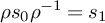 and
$\rho s_1 \rho ^{-1} =s_0$
 .
The extended affine Hecke algebra
$\widehat {H}^{\mathrm {ext}}_{2}$
 is generated by
$T_0, T_1$
 and
$\rho ^{\pm 1}$
 , subject to only the first relation in (8) and all relations in (9). In this case, it is easy to express the KL basis elements
$b_w$
 in terms of the regular basis elements
$T_u$
 explicitly:

where
$\preceq $
 denotes the Bruhat order on
$\widehat {\mathfrak {S}}_2$
 . Note that
$u \preceq w$
 holds iff the rex for u is an alternating binary subsequence of the rex for w and it is easy to invert this change of basis:

The multiplication constants w.r.t. the KL basis are also easy to compute in this case and are all equal to 0, 1, 2 or
$[2]=q+q^{-1}$
 . For
$m,n\in \mathbb {Z}_{\geq 1}$
 (assuming that the parity conditions are met in each line below), we have

and the analogous equations with
$0$
 and
$1$
 swapped. These formulas are certainly known to experts, but we couldn’t find an explicit reference for all of them in the literature (the first formula can be found in [Reference LusztigLus, Proposition 7.7(a)]). Let us, therefore, briefly explain how we obtained them. There is a close relation between
$\widehat {H}^{\mathrm {ext}}_{2}$
 and a two-coloured version of the Grothendieck ring of finite-dimensional representations (of type I) of quantum
$\mathfrak {sl}_2$
 , see [Reference EliasEli1, Section 2.2.1]. In the first four cases above, when the last element of the left alternating binary sequence and the first element of the right alternating binary sequence are equal, this correspondence is given by the bijection

where
$[V_{m-1}]$
 is the Grothendieck class of the (essentially unique) m-dimensional irreducible representation of quantum
$\mathfrak {sl}_2$
 . Note that the Grothendieck ring over
$\mathbb {Z}$
 must be tensored with
$\mathbb {Z}[q,q^{-1}]$
 for multiplication by
$[2]$
 to make sense. In the first case, for example, we get

where we have used the well-known Clebsch-Gordan rule for the decomposition of the tensor product of two finite-dimensional irreducible representations of quantum
$\mathfrak {sl}_2$
 . It is well-known that
$b_i b_{{}_{i}\widehat {m}_{\,j}}=b_{{}_{i}\widehat {m}_{\,j}} b_j = [2] b_{{}_{i}\widehat {m}_{\,j}}$
 , for
$m\in \mathbb {Z}_{\geq 1}$
 and
$i,j\in \{0,1\}$
 satisfying the parity condition. The remaining cases above can be reduced to the first four cases (sometimes with
$0$
 and
$1$
 swapped) by that basic multiplication rule and a simple trick, assuming (just for the sake of this trick) that we work over
$\mathbb {Q}(q)$
 for example. Suffice it to give an illustrative example:

where we use the equality
$b_1 b_{{}_{0}\widehat {n}_{\,1}}=b_{{}_{1}\widehat {n+1}_{\,1}}+ b_{{}_{1}\widehat {n-1}_{\,1}}$
 , which is the special case of the fifth equation in (123) for
$m=1$
 .
Recall the standard trace
$\epsilon \colon \widehat {H}^{\mathrm {ext}}_{2}\to \mathbb {Z}[q,q^{-1}]$
 from (16) and the associated q-sesquilinear form
$(-,-)$
 on
$\widehat {H}^{\mathrm {ext}}_{2}$
 from (17). The formula in (121) implies that

for any
$w\in \widehat {\mathfrak {S}}_n$
 . Note further that
$\omega (b_{{}_{i}\widehat {m}_{\,j}})=b_{{}_{j}\widehat {m}_{\,i}}$
 , for
$m\in \mathbb {Z}_{\geq 0}$
 and
$i,j\in \{0,1\}$
 . The following lemma, which is an immediate consequence of the above, is a more detailed version of Theorem 2.2 in this particular case and will be needed in Section 5.3.
Lemma 5.1. For any
$r,s\in \mathbb {Z}$
 and
$i,j,k,l\in \{0,1\}$
 , we have
$(\rho ^r b_{{}_{i}\widehat {m}_{\,j}}, \rho ^s b_{{}_{k}\widehat {n}_{\,l}})=\delta _{r,s} (b_{{}_{i}\widehat {m}_{\,j}}, b_{{}_{k}\widehat {n}_{\,l}})$
 and

where
$p(q), p'(q)\in \mathbb {Z}_{\geq 0}[q]$
 have constant terms equal to two and to one, respectively.
5.1.2 Two representations of
$\widehat {H}^{\mathrm {ext}}_{2}$

Let
$V=\mathrm {Span}\{v\}$
 be the trivial one-dimensional
$\widehat {H}^{\mathrm {ext}}_{1}$
 -module, defined by

and let

the Zelevinsky tensor product of V with itself. Recall from Section 1 that

Recall also that

where
$\rho \in \widehat {H}^{\mathrm {ext}}_{2}$
 . Thus, for any
$r,s\in \mathbb {Z}$
 , we have

This implies that W is two-dimensional and that
$\{w,w'\}$
 , where

is a basis of W, on which the action of
$\widehat {H}^{\mathrm {ext}}_{2}$
 is given by the matrices

On the KL-basis, the action thus becomes

Using the rules for multiplication w.r.t. the KL-basis, we see that the action matrices satisfy:

Recall that q is a formal invertible parameter and let
${-}^{\mathbb {C}(q)}:={-}\otimes _{\mathbb {Z}[q,q^{-1}]}\mathbb {C}(q)$
 . The following result is well-known, see e.g. [Reference Leclerc, Nazarov and ThibonLNT, Theorem 1].
Proposition 5.2. The
$\widehat {H}^{\mathrm {ext},\mathbb {C}(q)}_{2}$
 -module
$W^{\mathbb {C}(q)}$
 is simple.
There is also an infinite-dimensional
$\widehat {H}^{\mathrm {ext}}_{2}$
 -module U which is closely related to W and whose categorification will be important below. By definition,

the quotient of the regular left
$\widehat {H}^{\mathrm {ext}}_{2}$
 -module by the left ideal I generated by

Remark 5.3. We stress that I is only a left ideal and not a two-sided ideal. For
$\rho ^2 -1$
 this distinction is irrelevant, because
$\rho ^2$
 and
$1$
 both belong to the centre of
$\widehat {H}^{\mathrm {ext}}_{2}$
 , but for
$b_1\rho - q^{-1}b_1$
 it matters. For example, the element
$(1-q^{-2})b_1$
 belongs to the two-sided ideal generated by the elements in (127) because

but it does not belong to I.
Proposition 5.4. Let
$\pi _U\colon \widehat {H}^{\mathrm {ext}}_{2}\to U$
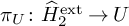 be the natural projection and define
$u_k:=\pi _U(b_{\widehat {k}_{\,1}})$
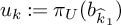 and
$u^{\prime }_k:=\pi _U(\rho b_{\widehat {k}_{\,1}})$
 , for all
$k\in \mathbb {Z}_{\geq 0}$
 . Then
$\{u_k, u^{\prime }_k\mid k\in \mathbb {Z}_{\geq 0}\}$
 is a basis of U and the action of
$\widehat {H}^{\mathrm {ext}}_{2}$
 on this basis is determined by

for
$k\in \mathbb {Z}_{\geq 1}$
 .
Proof. To show that
$\{u_k, u^{\prime }_k\mid k\in \mathbb {Z}_{\geq 0}\}$
 spans U is easy. The KL-basis of
$\widehat {H}^{\mathrm {ext}}_{2}/\langle \rho ^2 -1 \rangle $
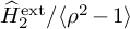 , where
$\langle \rho ^2 - 1\rangle $
 is the (left) ideal generated by
$\rho ^2-1$
 , is given by
$\{\rho ^m b_{\widehat {k}_{\,1}}, \rho ^m b_{\widehat {k}_{\,0}}\mid m\in \{0,1\}, k\in \mathbb {Z}_{\geq 0}\}$
 . The images of those elements under
$\pi _U$
 , therefore, span U. By induction, it’s easy to show that
$b_{\widehat {k}_{\,1}}\rho - q^{-1} b_{\widehat {k}_{\,1}}\in I$
 for all
$k\in \mathbb {Z}_{>0}$
 . For
$k=2$
 , we have

For
$k>2$
 , induction yields

This shows that
$\rho b_{\widehat {k}_{\,0}}= b_{\widehat {k}_{\,1}}\rho =q^{-1} b_{\widehat {k}_{\,1}}$
 in U, for all
$k\in \mathbb {Z}_{\geq 0}$
 . This in turn implies that
$b_{\widehat {k}_{\,0}}=\rho ^2 b_{\widehat {k}_{\,0}}=q^{-1} \rho b_{\widehat {k}_{\,1}}$
 , for all
$k\in \mathbb {Z}_{\geq 0}$
 , which completes the proof that
$\{u_k, u^{\prime }_k\mid k\in \mathbb {Z}_{\geq 0}\}$
 spans U.
It remains to prove that the elements
$u_k, u^{\prime }_k$
 , for
$k\in \mathbb {Z}_{\geq 0}$
 , are all linearly independent in U. Suppose that

for some
$r,s\in \mathbb {Z}_{\geq 0}$
 and some
$\mu _{m_1},\ldots , \mu _{m_r},\nu _{n_1}\ldots , \nu _{n_s}\in \mathbb {k}$
 . Then

Since
$b_1\rho = \rho b_0$
 , any non-zero element in I will be a linear combination of KL basis elements containing at least a non-zero multiple of
$\rho b_{\widehat {k}_{\,0}}$
 , for some
$k\in \mathbb {Z}_{> 0}$
 , or a non-zero multiple of
$\rho ^2 b_{\widehat {k}_{\,i}}$
 , for some
$k\in \mathbb {Z}_{\geq 0}$
 and
$i\in \{0,1\}$
 . Either way, linear independence of the KL basis elements in
$\widehat {H}^{\mathrm {ext}}_{2}$
 implies that (129) can only hold if
$\lambda _{m_1} b_{\widehat {m_1}_{\,1}} + \ldots + \lambda _{m_r} b_{\widehat {m_r}_{\,1}} + \mu _{n_1} \rho b_{\widehat {n_1}_{\,1}} + \ldots + \mu _{n_s} \rho b_{\widehat {n_s}_{\,1}}=0$
 and, therefore, that
$\lambda _{m_i}=\mu _{n_j}=0$
 for all
$i=1,\ldots , r$
 and
$j=1,\ldots , s$
 . This completes the proof that the elements
$u_k, u^{\prime }_k$
 , for
$k\in \mathbb {Z}_{\geq 0}$
 , are all linearly independent in U.
Finally, it is easy to determine the action of
$\rho , b_0$
 and
$b_1$
 on this basis using the KL multiplication rules, because
$\pi _U$
 is a morphism of
$\widehat {H}^{\mathrm {ext}}_{2}$
 -modules.
Let
$J\subset U$
 be the
$\widehat {H}^{\mathrm {ext}}_{2}$
 -submodule generated by
$T_1u_0-\rho u_0$
 and let
$\overline {u}\in U/J$
 be the image of
$u\in U$
 under the natural projection
$U\to U/J$
 . We have

Proposition 5.5. There is a surjective morphism of
$\widehat {H}^{\mathrm {ext}}_{2}$
 -modules

and
$\ker (\pi ^U_W)=J$
 .
Proof. Define
$\pi ^U_W\colon U\to W$
 by

extending it to the whole of U by the requirement that it be a morphism of
$\widehat {H}^{\mathrm {ext}}_{2}$
 -modules. Note that the matrices in (126) imply that

so
$\pi ^U_W$
 is well-defined.
The fact that
$\pi ^U_W(u_0)=w$
 and
$\pi ^U_W(u^{\prime }_0)=w'$
 proves that
$\pi ^U_W$
 is surjective.
It remains to show that
$\ker (\pi ^U_W)=J$
 . The matrices in (126) show that
$\rho T_1 w= w$
 , which implies that

so
$J\subseteq \ker (\pi ^U_W)$
 . To prove that this inclusion is an equality we will show that
$\dim _{\mathbb {k}}(U/J)=2$
 , which amounts to showing that
$\overline {u_k}, \overline {u^{\prime }_k}\in \mathrm {span}\{\overline {u_0}, \overline {u^{\prime }_0}\}$
 for all
$k\in \mathbb {Z}_{\geq 0}$
 . We will prove this by induction. Recall that
$b_i=T_i+q$
 , for
$i\in \{0,1\}$
 . Then, for the base step, we have

For the inductive step, let
$k>2$
 and assume that that
$\overline {u_m}, \overline {u^{\prime }_m}\in \mathrm {span}\{\overline {u_0}, \overline {u^{\prime }_0}\}$
 for all
$0\leq m< k$
 . If
$k>2$
 is odd, then

By induction, the elements
$\overline {u_{k-1}}, \overline {u_{k-2}}$
 belong to
$\mathrm {span}\{\overline {u_0}, \overline {u^{\prime }_0}\}$
 . Since
$\overline {b_1 u_0}=\overline {u_1}=\overline {u^{\prime }_0+qu_0}$
 and
$\overline {b_1 u^{\prime }_0}=q^{-1} \overline {u_1}=\overline {q^{-1}u^{\prime }_0+ u_0}$
 , we conclude that
$\overline {u_k}\in \mathrm {span}\{\overline {u_0}, \overline {u^{\prime }_0}\}$
 . If
$k>2$
 is even, then

By induction again, the elements
$\overline {u_{k-1}}, \overline {u_{k-2}}$
 belong to
$\mathrm {span}\{\overline {u_0}, \overline {u^{\prime }_0}\}$
 . Since
$\overline {b_0 u_0}=\overline {q^{-1} u^{\prime }_1}=\overline {q^{-1} u_0+u^{\prime }_0}$
 and
$\overline {b_0 u^{\prime }_0}=\overline {u^{\prime }_1}=\overline {u_0+qu^{\prime }_0}$
 , we conclude that
$\overline {u_k}\in \mathrm {span}\{\overline {u_0}, \overline {u^{\prime }_0}\}$
 . This completes the proof that
$u_k$
 belongs to
$\mathrm {span}\{\overline {u_0}, \overline {u^{\prime }_0}\}$
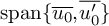 for all
$k\in \mathbb {Z}_{\geq 0}$
 . Using similar arguments, one can show that the same also holds for
$u^{\prime }_k$
 , for all
$k\in \mathbb {Z}_{\geq 0}$
 , which concludes the proof.
Just to fix notation, let
$\pi _W\colon \widehat {H}^{\mathrm {ext}}_{2}\to W$
 be the projection of
$\widehat {H}^{\mathrm {ext}}_{2}$
 -modules defined by
$\pi _W(x):=xw$
 , for any
$x\in \widehat {H}^{\mathrm {ext}}_{2}$
 . Then there is a commutative triangle

Remark 5.6. The infinite-dimensional representation U of
$\widehat {H}^{\mathrm {ext}}_{2}$
 is the decategorification of a wide finitary birepresentation
$\mathbf {U}$
 of
${\widehat {\mathscr {S}}}^{\mathrm {ext}}_2$
 , which appears naturally as the wide finitary cover of the induced birepresentation
$\mathbf {W}$
 in Section 5.3. However, we do not know if U also appears naturally in any approach to the representation theory of
$\widehat {H}^{\mathrm {ext}}_{2}$
 that does not use categorification. Note that this contrasts with the finitary cover
$\widehat {\mathbf {M}}_{r,s}$
 (
$r,s\in \mathbb {Z}$
 ) of the evaluation birepresentation
$\mathbf {M}^{\mathcal {E}v_{r,s}}$
 of
${\widehat {\mathscr {S}}}^{\mathrm {ext}}_n$
 in [Reference Mackaay, Miemietz and VazMMV, Corollary 6.5], which decategorifies to a Graham-Lehrer cell module of
$\widehat {H}^{\mathrm {ext}}_{n}$
 , see [Reference Mackaay, Miemietz and VazMMV, Remark 6.6].
5.2 Completions of linear additive categories
In this subsection, we lay the groundwork for studying the application of our embedding to the induction of birepresentations. Roughly speaking, birepresentations over an additive bicategory correspond to algebras in some completion of the latter and one can define induction from one bicategory to another by pushing forward the algebras through an appropriate embedding. In our case, the situation is rather delicate as we move between additive and triangulated bicategories, so in this section we carefully study the completions in which our algebras live, both in the additive and triangulated world. Since this section is more general, we will work over an arbitrary field and with bicategories rather than monoidal categories.
5.2.1 Coproduct completions of additive
$\mathbb {k}$
-linear categories

Let
$\mathcal {C}$
 be an additive
$\mathbb {k}$
 -linear category. Recall that the additive closure
$\mathrm {add}(\mathcal {A})$
 of a full subcategory
$\mathcal {A}$
 of
$\mathcal {C}$
 is the closure under direct sums and direct summands in
$\mathcal {C}$
 .
We note that
$\mathrm {Vect}_{\mathbb {k}}$
 is complete and cocomplete with respect to small weighted (and hence, in particular, conical) limits and colimits. This follows from [Reference RiehlRie, Corollary 7.6.4] using [Reference RiehlRie, Example 3.7.5] and the fact that
$\mathrm {Vect}_{\mathbb {k}}$
 is enriched over itself.
This implies that the category of
$\mathbb {k}$
 -linear functors
${\mathcal {C}}^\circ =\mathsf {{F}} un_{\mathbb {k}}(\mathcal {C}^{op},\mathrm {Vect}_{\mathbb {k}})$
 , is also (co)complete under weighted (co)limits by [Reference KellyKel, Section 3.3] with (co)limits being computed object-wise. As usual, we identify an object X in
$\mathcal {C}$
 with their representables
$X^\vee =\mathrm {Hom}_{\mathcal {C}}( -, X)$
 under the Yoneda embedding. We denote by
$\mathcal {C}^\vee $
 the image of
$\mathcal {C}$
 under this embedding (which is, of course, equivalent to
$\mathcal {C}$
 ).
Note that we can realise a (co)product indexed by a set J as the conical (co)limit over the diagram
$J \to \mathcal {C}\colon j \mapsto X_j$
 . This is a special case of the weighted (co)limit of the
$\mathrm {Vect}_{\mathbb {k}}$
 -enriched functor
$\tilde J \to \mathcal {C}$
 where
$\tilde J$
 is the free
$\mathrm {Vect}_{\mathbb {k}}$
 -enriched category on J and the weight
$\tilde J\to \mathrm {Vect}_{\mathbb {k}}$
 is just the constant functor
$j\mapsto \mathbb {k}$
 . For a family of objects
$(X_j)_{j\in J}$
 in
$\mathcal {C}$
 , we slightly abuse notation by writing
$\coprod _{j\in J}X_j$
 for said colimit in
${\mathcal {C}}^\circ $
 rather than the formally correct
$\coprod _{j\in J}X_j^\vee $
 and likewise for products.
Since
$\mathcal {C}$
 and hence
${\mathcal {C}}^\circ $
 is additive, in particular has a zero object, there is always a canonical monomorphism

Explicitly, denoting by
$\pi _i \colon \prod _{j\in J } X_j\to X_i$
 and
$\iota _i\colon X_i \to \coprod _{j\in J } X_j$
 the canonical projections and injections, respectively,
$\nu $
 is defined by the condition that

We define
${\mathcal {C}}^\sqcup $
 as the full subcategory of
${\mathcal {C}}^\circ $
 where we close
$\mathcal {C}^\vee $
 under countable coproducts. We then denote by
${\mathcal {C}}^\diamond =({\mathcal {C}}^\sqcup )_e$
 its Karoubi envelope. Note that both are again additive
$\mathbb {k}$
 -linear categories. Moreover,
${\mathcal {C}}^\diamond $
 is closed under countable coproducts. We observe that, by [Reference BreazBre, Theorem 4.1],
${\mathcal {C}}^\diamond $
 and
${\mathcal {C}}^\sqcup $
 coincide provided
$\mathcal {C}$
 is Krull-Schmidt.
A
$\mathbb {k}$
 -linear functor
$\mathrm {F}\colon \mathcal {C}\to \mathcal {D}$
 between additive
$\mathbb {k}$
 -linear categories induces
$\mathbb {k}$
 -linear functors, also denoted by
$\mathrm {F}$
 , from
${\mathcal {C}}^\sqcup \to {\mathcal {D}}^\sqcup $
 , sending an object
$\coprod _{j\in J}X_j$
 to
$\coprod _{j\in J}\mathrm {F}(X_j)$
 , and hence from
${\mathcal {C}}^\diamond \to {\mathcal {D}}^\diamond $
 .
The next lemma will be crucial for computing morphism spaces in explicit examples.
Lemma 5.7. Assume
$Y=\coprod _{j\in J} Y_j \in {\mathcal {C}}^\circ $
 , where each
$Y_j\in \mathcal {C}$
 . Let
$X\in \mathcal {C}$
 and assume that
$\mathrm {Hom}_{\mathcal {C}}(X,Y_j)= 0$
 for all but finitely many
$j\in J$
 . Then
$\mathrm {Hom}_{{\mathcal {C}}^\circ }(X, Y) = \coprod _{j\in J}\mathrm {Hom}_{\mathcal {C}}(X,Y_j)$
 .
Proof. Consider the natural monomorphism

and compose this with the monomorphism induced by
$\nu = \nu _{(Y_j)_{j\in J}},$
 i.e.

The coproduct in the domain and the product in the codomain are both finite and hence isomorphic, so this monomorphism is an isomorphism. In particular,
$\kappa $
 is an isomorphism. The lemma now follows from the fact that
$\mathrm {Hom}_{{\mathcal {C}}^\circ }(X, Y_j ) = \mathrm {Hom}_{\mathcal {C}}(X,Y_j)$
 by the Yoneda Lemma.
Given that the (co)product of the morphism spaces in Lemma 5.7 is really finite, we write it as

5.2.2 Coproduct completions and homotopy categories
For a
$\mathbb {k}$
 -linear additive category
$\mathcal {C}$
 , we can consider the category
$C^b(\mathcal {C})$
 of bounded complexes over
$\mathcal {C}$
 and its completion
${C^b(\mathcal {C})}^\sqcup $
 under countable coproducts, and the Karoubi envelope
${C^b(\mathcal {C})}^\diamond $
 of the latter. Similarly, we can consider
$C^b({\mathcal {C}}^\sqcup )$
 and
$C^b({\mathcal {C}}^\diamond )$
 .
For reference, we record the following lemma, for which we could not find a proof in the literature.
Lemma 5.8. For an idempotent complete
$\mathbb {k}$
 -linear additive category
$\mathcal {C}$
 , the category
$C^b(\mathcal {C})$
 is idempotent complete.
Proof. Assume
$e^\bullet $
 is an idempotent endomorphism of an object
$(X^\bullet , d^\bullet )$
 in
$C^b(\mathcal {C})$
 . In particular, each
$e^i$
 is an idempotent endormorphism of
$X^i$
 . Since
$\mathcal {C}$
 is idempotent complete,
$X^i$
 splits into a direct sum of object
$X^i_{e}$
 and
$X^i_{1-e}$
 . Since
$e^\bullet $
 commutes with the differential
$d^\bullet $
 , each of these summands is preserved under the differential and the complex
$(X^\bullet , d^\bullet )$
 splits into a direct sum of complexes
$(X_e^\bullet , e^\bullet d^\bullet e^\bullet )$
 and
$(X^\bullet , (1-e)^\bullet d^\bullet (1-e)^\bullet )$
 .
Note that the Yoneda embedding
$\mathcal {C}\xrightarrow {\Upsilon } {\mathcal {C}}^\diamond $
 extends to an embedding
$C^b(\mathcal {C})\hookrightarrow C^b({\mathcal {C}}^\diamond )$
 , which gives rise to an embedding
${C^b(\mathcal {C})}^\diamond \hookrightarrow {C^b({\mathcal {C}}^\diamond )}^\diamond $
 . The following lemma is straightforward, noticing that a countable coproduct of complexes, which each have countable coproducts of objects in each component, is again a complex with countable coproducts in each component.
Lemma 5.9.
$C^b({\mathcal {C}}^\diamond )$
 is closed under countable coproducts, thus
$C^b({\mathcal {C}}^\diamond )\simeq {C^b({\mathcal {C}}^\diamond )}^\diamond $
 and we have an embedding
$\iota \colon {C^b(\mathcal {C})}^\diamond \hookrightarrow C^b({\mathcal {C}}^\diamond )$
 .
Proof. Let
$(X_i^\bullet , d_i^\bullet )_{i\in I}$
 be a family of objects in
$C^b({\mathcal {C}}^\diamond )$
 and consider the coproduct
$X=\coprod _{i\in I}(X_i^\bullet , d_i^\bullet )$
 in
${C^b({\mathcal {C}}^\diamond )}^\sqcup $
 . Now define
$Y=(Y^\bullet , d^\bullet )$
 in
$C^b({\mathcal {C}}^\diamond )$
 as the complex whose kth component is given by
$\coprod _{i\in I}X_i^k$
 and whose differential
$d^k$
 is given by
$\coprod _{i\in I}X_i^k\xrightarrow {(d_i^k)_{i\in I}}\coprod _{i\in I}X_i^{k+1}$
 . Then clearly,
$Y\cong X$
 , so
$C^b({\mathcal {C}}^\diamond )$
 is closed under coproducts and
$C^b({\mathcal {C}}^\diamond )\simeq {C^b({\mathcal {C}}^\diamond )}^\sqcup $
 . Since by Lemma 5.8,
$C^b({\mathcal {C}}^\diamond )$
 is idempotent complete,
$C^b({\mathcal {C}}^\diamond )\simeq {C^b({\mathcal {C}}^\diamond )}^\diamond $
 .
Denote by
$N^b(\mathcal {C})\subset C^b(\mathcal {C})$
 the ideal of nulhomotopic morphisms of complexes, and by
$K^b(\mathcal {C}) = C^b(\mathcal {C})/N^b(\mathcal {C})$
 the bounded homotopy category.
Observe that the fully faithful functor
$C^b(\mathcal {C})\hookrightarrow C^b({\mathcal {C}}^\diamond )$
 induced by the Yoneda embedding preserves nullhomotopic maps, and we thus obtain a fully faithful functor
$K^b(\mathcal {C})\hookrightarrow K^b({\mathcal {C}}^\diamond )$
 . Morover,
$\iota $
 also preserves nullhomotopic morphisms so we also obtain a fully faithful functor
$ {K^b(\mathcal {C})}^\diamond \to K^b({\mathcal {C}}^\diamond )$
 , which we again denote by
$\iota $
 .
Corollary 5.10.
-
(a) We have fully faithful functors $K^b(\mathcal {C})\xrightarrow {K^b(\Upsilon )}{K^b(\mathcal {C})}^\diamond \xrightarrow {\iota } K^b({\mathcal {C}}^\diamond )$
. -
(b) If $\mathcal {D}$
is a
$\mathbb {k}$
-linear additive category, a
$\mathbb {k}$
-linear functor
$\Phi \colon \mathcal {C}\to K^b(\mathcal {D})$
induces a
$\mathbb {k}$
-linear functor
${\mathcal {C}}^\diamond \to K^b({\mathcal {D}}^\diamond )$
.


Proof. The first part is immediate. For the second part, note that
$\Phi $
 gives rise to a functor
${\mathcal {C}}^\diamond \to {K^b(\mathcal {D})}^\diamond $
 . Composing this with the inclusion from the first part yields the desired functor
${\mathcal {C}}^\diamond \to K^b({\mathcal {D}}^\diamond )$
 .
5.2.3 Wide finitary bicategories
Here we recall some of the definitions from [Reference MacphersonMacph]. Remember that a
$2$
 -category is a strict bicategory, meaning that all coherence morphisms are identities. We will generally be speaking about bicategories, but some of these happen to be
$2$
 -categories.
Denote by
$\mathfrak {A}_{\mathbb {k}}$
 the
$2$
 -category whose objects are additive
$\mathbb {k}$
 -linear categories, whose
$1$
 -morphisms are
$\mathbb {k}$
 -linear functors and whose
$2$
 -morphisms are natural transformations.
A category
$\mathcal {C}$
 is wide finitary if it is an additive
$\mathbb {k}$
 -linear Krull–Schmidt category with at most countably many isomorphism classes of indecomposable objects and morphism spaces of at most countable dimension. We denote by
$\mathrm {\mathrm {ind}}{\mathcal {C}}$
 a set of representatives of isomorphism classes of indecomposable objects in
$\mathcal {C}$
 .
We denote the
$2$
 -category whose objects are wide finitary categories, whose
$1$
 -morphisms are
$\mathbb {k}$
 -linear functors, and whose
$2$
 -morphisms are natural transformations by
$\mathfrak {A}^{wf}_{\mathbb {k}}$
 .
We say that a bicategory
$\mathcal {C}$
 is wide finitary if
-
• it has finitely many objects;
-
• $\mathcal {C}(\mathtt {i},\mathtt {j})$
is in
$\mathfrak {A}^{wf}_{\mathbb {k}}$
for all
$\mathtt {i},\mathtt {j} \in \mathcal {C}$
; -
• horizontal composition is biadditive and $\mathbb {k}$
-linear; -
• the identity $1$
-morphism
$\mathbb {1}_{\mathtt {i}}$
is indecomposable for any
$\mathtt {i}\in \mathcal {C}$
.


We use
$\circ _{\mathsf {h}}$
 , resp.
$\circ _{\mathsf {v}}$
 , for horizontal, respectively vertical, composition in a bicategory.
Recall that if
$\mathcal {C}$
 is a bicategory,
$\mathcal {C}^{\mathsf {co},\mathsf {op}}$
 is the bicategory obtained by reversing the direction of both
$1$
 - and
$2$
 -morphisms. A wide finitary bicategory
$\mathcal {C}$
 is said to be wide fiat if there exists a weak involution
$(-)^*\colon \mathcal {C}\to \mathcal {C}^{\mathsf {co},\mathsf {op}}$
 such that, for any
$1$
 -morphism
$\mathrm {F}\in \mathcal {C}(\mathtt {i},\mathtt {j})$
 , there are natural
$2$
 -morphisms
$\alpha \colon \mathrm {F}\mathrm {F}^* \to \mathbb {1}_{\mathtt {j}}, \beta \colon \mathbb {1}_{\mathtt {i}}\to \mathrm {F}^*\mathrm {F}$
 satisfying the usual adjunction triangles, i.e.
$(\alpha \circ _{0}\mathrm {\mathrm {Id}}_{\mathrm {F}})\circ _1 (\mathrm {\mathrm {Id}}_{\mathrm {F}} \circ _0\beta ) = \mathrm {\mathrm {Id}}_{\mathrm {F}}$
 and
$(\beta \circ _0\mathrm {\mathrm {Id}}_{\mathrm {F}^*})\circ _1(\mathrm {\mathrm {Id}}_{\mathrm {F}^*}\circ _0\alpha )=\mathrm {\mathrm {Id}}_{\mathrm {F}^*}$
 .
Note that
${\widehat {\mathscr {S}}}^{\mathrm {ext}}_n$
 is a wide fiat bicategory, where the fiat structure is defined by rotating the diagrams in Soergel calculus by 180 degrees and the adjunctions
$\alpha $
 and
$\beta $
 are defined by cups and caps, respectively.
5.2.4 Completed and triangulated bicategories
Let
$\mathcal {C}$
 be a wide finitary bicategory. We define the bicategory
${\mathcal {C}}^\diamond $
 to be the bicategory on the same objects as
$\mathcal {C}$
 , but with morphism categories
${\mathcal {C}}^\diamond (\mathtt {i},\mathtt {j}) ={ \mathcal {C}(\mathtt {i},\mathtt {j})}^\diamond (={ \mathcal {C}(\mathtt {i},\mathtt {j})}^\sqcup )$
 , with horizontal composition given componentwise, i.e.

and similarly for 2-morphisms. Observe that
${\mathcal {C}}^\diamond $
 is locally additive and
$\mathbb {k}$
 -linear.
Remark 5.11. Note that this naturally embeds into the completion
${\mathcal {C}}^\circ $
 with morphism categories
${\mathcal {C}}^\circ (\mathtt {i},\mathtt {j}) ={ \mathcal {C}(\mathtt {i},\mathtt {j})}^\circ $
 and horizontal composition given by Day convolution.
Likewise, for any locally additive
$\mathbb {k}$
 -linear (or in particular wide finitary) bicategory
$\mathcal {C}$
 , we can define
$K^b(\mathcal {C})$
 as having the same objects as
$\mathcal {C}$
 , morphism categories
$K^b(\mathcal {C})(\mathtt {i},\mathtt {j})=K^b(\mathcal {C}(\mathtt {i},\mathtt {j}))$
 and horizontal composition induced by taking the total complex of the tensor product of complexes. This is a triangulated bicategory, which fits within the bicategorical version of the framework considered in [Reference Laugwitz and MiemietzLaMi, Section 3.1].
Lemma 5.12. If
$\mathcal {C}$
 is wide finitary and all
$1$
 -morphisms have finite-dimensional endomorphism rings, then
$K^b(\mathcal {C})$
 is wide finitary.
Proof. Since
$\mathcal {C}$
 is locally idempotent complete, so is
$K^b(\mathcal {C})$
 by [Reference SchnürerSch, Theorem 3.4]. Since endomorphism rings of
$1$
 -morphisms in
$\mathcal {C}$
 are finite-dimensional, the same is true for endomorphism rings of
$1$
 -morphisms in
$K^b(\mathcal {C})$
 . Thus
$K^b(\mathcal {C})$
 is Krull-Schmidt by [Reference KrauseKra, Cor 4.4]. Countability of isomorphism classes of indecomposables is inherited from
$\mathcal {C}$
 .
Corollary 5.13. For any
$n\in \mathbb {Z}_{\geq 2}$
 , the monoidal category (one-object bicategory)
$K^b({\widehat {\mathscr {S}}}^{\mathrm {ext}}_n)$
 is wide finitary.
5.2.5 Birepresentations
An additive birepresentation of a locally additive
$\mathbb {k}$
 -linear bicategory
$\mathcal {C}$
 is a
$\mathbb {k}$
 -linear pseudofunctor from
$\mathcal {C}$
 to
$\mathfrak {A}_{\mathbb {k}}$
 . A wide finitary birepresentation of a wide finitary bicategory
$\mathcal {C}$
 is a
$\mathbb {k}$
 -linear pseudofunctor from
$\mathcal {C}$
 to
$\mathfrak {A}^{wf}_{\mathbb {k}}$
 .
We can extend an additive or wide finitary birepresentation
$\mathbf {M}$
 of
$\mathcal {C}$
 to an additive birepresentation
${\mathbf {M}}^\diamond $
 of
${\mathcal {C}}^\diamond $
 by defining the action of
$\mathrm {F}=\coprod _{i\in I}\mathrm {F}_i \in { \mathcal {C}}^\diamond (\mathtt {i},\mathtt {j})$
 on
$X =\coprod _{j\in J}X_j \in {\mathbf {M}}^\diamond (\mathtt {i})$
 componentwise, i.e.

Similarly, any additive birepresentation of
$\mathbf {M}$
 gives rise to a triangulated birepresentation
$K^b(\mathbf {M})$
 of
$K^b(\mathcal {C})$
 where
$K^b(\mathbf {M})(\mathtt {i}) = K^b(\mathbf {M}(\mathtt {i}))$
 .
5.2.6 Algebras and birepresentations in
${\mathcal {C}}^\diamond $

Let
$\mathcal {C}$
 be a wide finitary bicategory.
Now assume G is an abelian group and
$\mathrm {Y} = \coprod _{j\in G} \mathrm {Y}_j\in {\mathcal {C}}^\diamond (\mathtt {i},\mathtt {i})$
 is an algebra
$1$
 -morphism with product

determined by component morphisms
$\mathbf {m}_{i,j} = \mathbf {m} (\iota _i\circ _{\mathsf {h}}\iota _j) \colon \mathrm {Y}_i\mathrm {Y}_j \to \mathrm {Y}_{i+j}$
 , where we identify
$\mathrm {Y}_{i+j}$
 with the subobject of
$\coprod _{k\in G} \mathrm {Y}_k$
 given by
$\iota _{i+j}(\mathrm {Y}_{i+j})$
 , and unit
$\mathbf {u}$
 determined by a morphism
$\mathbb {1}_{\mathtt {i}}\to \mathrm {Y}_0$
 , where
$0$
 is the neutral element in G.
For each
$\mathtt {j}\in \mathcal {C}$
 , we can consider the category of
$\mathrm {Y}$
 -modules in
${\mathcal {C}}^\diamond (\mathtt {i},\mathtt {j})$
 , denoted by
$\mathrm {mod}_{{\mathcal {C}(\mathtt {i},\mathtt {j})}^\diamond }\mathrm {Y}$
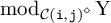 , which gives rise to an additive birepresentation
$\boldsymbol {\mathrm {mod}}_{{\mathcal {C}}^\diamond }\mathrm {Y}$
 of
${\mathcal {C}}^\diamond $
 . Note that each
$\mathrm {mod}_{{\mathcal {C}(\mathtt {i},\mathtt {j})}^\diamond }\mathrm {Y}$
 is idempotent complete by construction.
By the usual free forgetful adjunction, we have, for
$\mathrm {F}\in \mathcal {C}(\mathtt {i},\mathtt {i})$
 an isomorphism

Lemma 5.14. Let
$\mathrm {Y} = \coprod _{j\in G} \mathrm {Y}_j\in {\mathcal {C}}^\diamond (\mathtt {i},\mathtt {i})$
 be an algebra
$1$
 -morphism as above,
$\mathrm {F}\in \mathcal {C}(\mathtt {i},\mathtt {i})$
 and
$g\in \mathrm {Hom}_{{\mathcal {C}(\mathtt {i},\mathtt {i})}^\diamond } (\mathrm {F}, \mathrm {Y})$
 . Assume that g factors over
$\iota _j$
 , i.e. there exists an
$g_j\in \mathrm {Hom}_{{\mathcal {C}(\mathtt {i},\mathtt {i})}} (\mathrm {F}, \mathrm {Y}_j)$
 such that
$g = \iota _j\circ _{\mathsf {v}} g_j$
 . Then under the isomorphism in (131), g corresponds to a morphism f defined by

Proof. This is a direct computation, observing that

so the claim follows.
Lemma 5.15. Let
$\mathcal {C}$
 be a wide finitary bicategory and
$\mathrm {Y}\in {\mathcal {C}(\mathtt {i},\mathtt {i})}^\diamond $
 an algebra
$1$
 -morphism. Assume that for any
$\mathrm {G}\in \mathcal {C}(\mathtt {i},\mathtt {i})$
 , the morphism space
$\mathrm {Hom}_{{\mathcal {C}(\mathtt {i},\mathtt {i})}^\diamond }(\mathrm {G}, \mathrm {Y})$
 is finite-dimensional. Then the birepresentation
$\mathbf {M}_{\mathrm {Y}}$
 given by
$\mathbf {M}_{\mathrm {Y}}(\mathtt {j}) = \mathrm {add}\{\mathrm {F} \mathrm {Y}\,\vert \, \mathrm {F}\in \mathcal {C}(\mathtt {i},\mathtt {j})\}$
 (where the additive closure is taken in
$\mathrm {mod}_{{\mathcal {C}(\mathtt {i},\mathtt {j})}^\diamond }\mathrm {Y}$
 ) is wide finitary.
Proof. By (131), for each
$\mathrm {F}\in \mathcal {C}(\mathtt {i},\mathtt {j})$
 , the endomorphism ring
$\mathrm {End}_{\mathrm {mod}_{{\mathcal {C}(\mathtt {i},\mathtt {j})}^\diamond }\mathrm {Y}}(\mathrm {F}\mathrm {Y})$
 is isomorphic to
$\mathrm {Hom}_{{\mathcal {C}(\mathtt {i},\mathtt {i})}^\diamond }(\mathrm {F}^*\mathrm {F}, \mathrm {Y})$
 , which by assumption is finite-dimensional. Since each
$\mathrm {mod}_{{\mathcal {C}(\mathtt {i},\mathtt {j})}^\diamond }\mathrm {Y}$
 is idempotent complete, [Reference KrauseKra, Cor 4.4] implies that each
$\mathbf {M}(\mathtt {j})$
 is Krull-Schmidt. Moreover, the number of isomorphism classes of indecomposable objects is countable and morphism spaces are even finite-dimensional, so
$\mathbf {M}_{\mathrm {Y}}$
 is wide finitary.
5.3 The categorified story
In the first part of this section, we will define a graded wide-finitary birepresentation
$\mathbf {U}$
 of
${\widehat {\mathscr {S}}}^{\mathrm {ext}}_2$
 and show that it categorifies the representation U of
$\widehat {H}^{\mathrm {ext}}_{2}$
 . In the second part, we will define a triangulated birepresentation
$\mathbf {W}$
 of
${\widehat {\mathscr {S}}}^{\mathrm {ext}}_2$
 and conjecture that it categorifies the representation W of
$\widehat {H}^{\mathrm {ext}}_{2}$
 .
5.3.1 The categorification of U
Let
$\mathbf {V}$
 be the rank one finitary
$2$
 -representation of
${\widehat {\mathscr {S}}}^{\mathrm {ext}}_1$
 categorifying V. The corresponding algebra object
$\mathrm {X}\in {\widehat {\mathscr {S}}}^{\mathrm {ext}, \diamond }_1$
 is given by

with multiplication
$\mu \colon \mathrm {X}\mathrm {X}\to \mathrm {X}$
 defined by the identity on
${\mathrm {B}}_{\rho }^k {\mathrm {B}}_{\rho }^{r-k}={\mathrm {B}}_{\rho }^r$
 , for all
$r,k\in \mathbb {Z}$
 , and unit
$\epsilon \colon \mathrm {I}\to \mathrm {X}$
 defined as the identity on
$\mathrm {I}={\mathrm {B}}_{\rho }^0$
 and zero to
${\mathrm {B}}_{\rho }^r$
 , for all
$r\ne 0$
 . Note that
$({\mathrm {B}}_{\rho })^k\cong {\mathrm {B}}_{\rho ^k}$
 and
$\mathrm {hom}_{{\widehat {\mathscr {S}}}^{\mathrm {ext}}_1}({\mathrm {B}}_{\rho ^k}\langle s\rangle , {\mathrm {B}}_{\rho ^m}\langle t\rangle )\cong \delta _{s,t}\delta _{k,m}\mathbb {R}$
 , for any
$k,m,s,t\in \mathbb {Z}$
 , where
$\delta _{-,-}$
 is the Kronecker delta.
Consider
$\mathrm {Y}:=\Psi _{1,1}(\mathrm {X}\boxtimes \mathrm {X})\in K^b({\widehat {\mathscr {S}}}^{\mathrm {ext}, \diamond }_2)$
 . The fact that
$\Psi _{1,1}$
 is a monoidal functor and the isomorphisms
${\mathrm {B}}_{\rho }\boxtimes {\mathrm {B}}_{\rho }\cong ({\mathrm {B}}_{\rho }\boxtimes \mathrm {I})(\mathrm {I}\boxtimes \mathrm {B}_{\rho })\cong (\mathrm {I}\otimes \mathrm {B}_{\rho })(\mathrm {B}_{\rho }\boxtimes \mathrm {I})$
 imply that

Note that, for any
$k,l\in \mathbb {Z}$
 , there are natural isomorphisms

because
$({\mathrm {B}}_\rho {\mathrm {T}}_1)^k$
 and
$ ({\mathrm {T}}_1^{-1} {\mathrm {B}}_\rho )^l$
 commute and

In particular, we see that

For any
$r,s\in \mathbb {Z}$
 , define

Lemma 5.16. Let
$i\in \{0,1\}$
 , and
$k,t\in \mathbb {Z}$
 , and
$m\in \mathbb {Z}_{\geq 0}$
 . Then

for all but finitely many
$r,s\in \mathbb {Z}$
 .
Proof. By [Reference Mackaay and ThielMaTh, Theorem 2.5], the hom-space in (133) is zero if
$r+s\ne k$
 . Now, assume that
$r+s=k$
 . We also assume that
$r\geq k$
 , the case
$r\leq k$
 being similar. Then

By biadjointness of
${\mathrm {B}}_{\rho ^k}$
 and
${\mathrm {B}}_{\rho ^{-k}}$
 , we have

which in turn is isomorphic to

where
${\mathrm {T}}_{\widehat {2r-k}_{\,1}}^{\min }$
 is the minimal complex obtained from
${\mathrm {T}}_{\widehat {2r-k}_{\,1}}$
 by Gaussian elimination, which is unique up to homotopy equivalence. By [Reference Elias and WilliamsonElWi1, Theorem 6.9], the degree-zero cochain object of
${\mathrm {T}}_{\widehat {2r-k}_{\,1}}^{\min }$
 is isomorphic to
${\mathrm {B}}_{\widehat {2r-k}_{\,1}}$
 , which implies that

For a fixed choice of
$m,t\in \mathbb {Z}$
 and
$m\in \mathbb {Z}_{\geq 0}$
 , Soergel’s hom formula and the equations in (123) imply that the latter morphism space is zero for all but finitely many
$r\in \mathbb {Z}$
 , which proves the lemma.
The following corollary is an immediate consequence of Lemma 5.7 and Lemma 5.16.
Corollary 5.17. For any
$i\in \{0,1\}$
 , and
$k,t\in \mathbb {Z}$
 , and
$m\in \mathbb {Z}_{\geq 0}$
 , there is an isomorphism

We are now going to define a graded wide finitary birepresentation
$\mathbf {U}$
 of
${\widehat {\mathscr {S}}}^{\mathrm {ext}}_2$
 and the rest of this section after the definition will be dedicated to the proof that it categorifies U.
Definition 5.18. Let

be the wide finitary birepresentation of
${\widehat {\mathscr {S}}}^{\mathrm {ext}}_2$
 generated by
$\mathrm {Y}$
 , as defined in Lemma 5.15.
Lemma 5.7 and the isomorphism in (131) imply that

where for simplicity we write
$\mathrm {hom}_{\mathrm {Y}}(\mathrm {A}\mathrm {Y}, {\mathrm {B}}\mathrm {Y})=\mathrm {hom}_{\mathrm {mod}_{K^b({\widehat {\mathscr {S}}}^{\mathrm {ext}, \diamond }_2)}\mathrm {Y}}(\mathrm {A}\mathrm {Y}, {\mathrm {B}}\mathrm {Y})$
 . The isomorphisms in (135) show that any morphism
$f\in \mathrm {hom}_{\mathrm {Y}}(\mathrm {A}\mathrm {Y}, {\mathrm {B}}\mathrm {Y})$
 is determined by its components
$f^{r,s}\in \mathrm {hom}_{K^b({\widehat {\mathscr {S}}}^{\mathrm {ext}}_2)}(\mathrm {A}, {\mathrm {B}}\mathrm {Y}^{r,s})$
 , for
$r,s\in \mathbb {Z}$
 . Suppose
$f\colon \mathrm {A}\mathrm {Y}\to BY$
 and
$g\colon {\mathrm {B}}\mathrm {Y}\to \mathrm {C}\mathrm {Y}$
 are such that their only nonzero components under the free forgetful adjunction are
$f^{r,s}\colon \mathrm {A}\to {\mathrm {B}}\mathrm {Y}^{r,s}$
 and
$g^{p,q}\colon {\mathrm {B}}\to \mathrm {C}\mathrm {Y}^{p,q}$
 . Then the only nonzero component of
$g\circ f\colon \mathrm {A}\mathrm {Y}\to \mathrm {C}\mathrm {Y}$
 under the free forgetful adjunction, is given by the composition

For morphisms with multiple nonzero components, this extends additively.
Proposition 5.19. Let
$k,m\in \mathbb {Z}_{\geq 0}$
 and
$r,s\in \mathbb {Z}$
 . When
$r\in \mathbb {Z}_{>0}$
 , the morphism spaces

are both zero for all
$t\geq 0$
 .
Proof. We only prove the first case, the proof of the second one being similar. Biadjointness and the isomorphism
${\mathrm {B}}_{\widehat {m}_{\,1}}^*\cong {\mathrm {B}}_{{}_{1}\widehat {m}}$
 imply that

By [Reference Mackaay and ThielMaTh, Theorem 2.5], that hom-space is zero if
$r+s\ne 0$
 , so suppose that
$r+s=0$
 . Then

Let
$r>0$
 . By [Reference Achar, Makisumi, Riche and WilliamsonAMRW, Section 9.1] (see also [Reference Elias and WilliamsonElWi1, Theorem 6.9] and [Reference Elias, Makisumi, Thiel and WilliamsonEMTW, Theorem 19.47]), the minimal complex
$[({\mathrm {T}}_0 {\mathrm {T}}_1)^r]^{\mathrm {min}}$
 is of the form

where the underlined cochain object has homological degree zero and the differential
$\mathrm {d}^{0}$
 is given by

where
$\mathrm {JW}_{(0,\ldots ,1)}$
 is the idempotent in
$\mathrm {end}_{{\widehat {\mathscr {S}}}^{\mathrm {ext}}_2}({\mathrm {B}}_0\cdots {\mathrm {B}}_1)$
 obtained from the Jones-Wenzl projector
$\mathrm {JW}_{2r}$
 by the quantum Satake correspondence, as in [Reference EliasEli1, Section 5.3.2] (see also [Reference Elias, Makisumi, Thiel and WilliamsonEMTW, Section 9.3]), and T denotes the transpose. Note that Elias and Williamson do not give the multiplicities of the indecomposables in positive homological degree, but in affine type
$A_1$
 both multiplicities in homological degree one can be deduced from the corresponding coefficients in (122). On the other hand, the formulas in (123) imply that the decomposition of
${\mathrm {B}}_{{}_{1}\widehat {m}}{\mathrm {B}}_{\widehat {k}_{\,1}}\langle t\rangle $
 only contains indecomposables of the form
${\mathrm {B}}_{{}_{1}\widehat {n}_{\,1}}\langle t+v \rangle $
 , with
$0\leq n\leq k+m$
 and
$v\in \{-1,0,1\}$
 . The parity conditions for
${}_{1}\widehat {n}_{\,1}$
 amount to n being odd. Any non-zero morphism of complexes in
$\mathrm {hom}_{K^b({\widehat {\mathscr {S}}}^{\mathrm {ext}}_2)}({\mathrm {B}}_{{}_{1}\widehat {m}}{\mathrm {B}}_{\widehat {k}_{\,1}}\langle t\rangle , [({\mathrm {T}}_0{\mathrm {T}}_1)^r]^{\mathrm {min}})$
 is given by a non-zero morphism in the morphism space
$\mathrm {hom}_{{\widehat {\mathscr {S}}}^{\mathrm {ext}}_2}({\mathrm {B}}_{{}_{1}\widehat {m}}{\mathrm {B}}_{\widehat {k}_{\,1}}\langle t\rangle , \mathrm {B}_{\widehat {2r}_{\,1}})$
 that is annihilated by postcomposition with the differential
$\mathrm {d}^0$
 . The latter morphism space is the direct sum of morphism spaces whose sources are the indecomposables of the form
${\mathrm {B}}_{{}_{1}\widehat {n}_{\,1}}\langle t+v \rangle $
 , with
$0\leq n\leq k+m$
 and
$v\in \{-1,0,1\}$
 , and Soergel’s hom formula in (49) and Lemma 5.1 imply that the graded rank of
$\mathrm {Hom}_{{\widehat {\mathscr {S}}}^{\mathrm {ext},*}_2}({\mathrm {B}}_{{}_{1}\widehat {n}_{\,1}}, {\mathrm {B}}_{\widehat {2r}_{\,1}})$
 is equal to

where
$p'(q)\in \mathbb {Z}_{\geq 0}[q]$
 has constant term equal to one. This implies that the morphism space
$\mathrm {hom}_{{\widehat {\mathscr {S}}}^{\mathrm {ext}}_2}({\mathrm {B}}_{{}_{1}\widehat {n}_{\,1}}\langle t+v\rangle , {\mathrm {B}}_{\widehat {2r}_{\,1}})$
 is zero unless
$t+v =-\vert n-2r\vert $
 . Suppose that
$t\geq 0$
 and recall that
$v\in \{-1,0,1\}$
 . Since n must be odd, we also see that
$\vert n-2r\vert>0$
 , so
$t+v =-\vert n-2r\vert $
 can only hold if
$t=0$
 ,
$v=-1$
 and
$\vert n-2r\vert =1$
 . In other words, the only non-zero morphism spaces are

which are both one-dimensional and generated by

respectively. However, neither of these two morphisms extends to a map of complexes whose target is
$[({\mathrm {T}}_0{\mathrm {T}}_1)^r]^{\mathrm {min}}$
 . To see this, note that postcomposition with
$\mathrm {d}^0$
 adds an extra dot to the rightmost, resp. leftmost, top strand of the morphisms in (140). These morphisms are all non-zero, because even with dots on all strands such morphisms are non-zero, see e.g. [Reference EliasEli1, Section 5.3.4] and [Reference Elias, Makisumi, Thiel and WilliamsonEMTW, (10.8i) and (10.9)]. This finishes the proof that

Corollary 5.20. For all
$k\in \mathbb {Z}_{\geq 0}$
 , the objects
${\mathrm {B}}_{\widehat {k}_{\,1}}\mathrm {Y}$
 and
${\mathrm {B}}_\rho {\mathrm {B}}_{\widehat {k}_{\,1}}\mathrm {Y}$
 are indecomposable in
$\mathbf {U}$
 .
Proof. The isomorphisms in (135) show that any non-zero idempotent
$e\in \mathrm {hom}_{\mathrm {Y}}({\mathrm {B}}_{\widehat {k}_{\,1}}\mathrm {Y}, {\mathrm {B}}_{\widehat {k}_{\,1}}\mathrm {Y})$
 is completely determined by its components
$e^{r,s}\in \mathrm {hom}_{K^b({\widehat {\mathscr {S}}}^{\mathrm {ext}}_2)}({\mathrm {B}}_{\widehat {k}_{\,1}}, {\mathrm {B}}_{\widehat {k}_{\,1}}\mathrm {Y}^{r,s})$
 , for
$r,s\in \mathbb {Z}$
 , and that only finitely many components are non-zero. By [Reference Mackaay and ThielMaTh, Theorem 2.5] and Proposition 5.19, we have
$e^{r,s}=0$
 unless
$r+s=0$
 and
$r\leq 0$
 . Furthermore,
$e^{0,0}$
 must be a multiple of the identity on
${\mathrm {B}}_{\widehat {k}_{\,1}}$
 , by Soergel’s hom formula in (49). By a slight abuse of notation, justified by Lemma 5.14, let us write
$e=e^{r_1,-r_1}+\ldots + e^{r_m,-r_m}$
 , for some
$r_i\in \mathbb {Z}_{\leq 0}$
 and
$m\in \mathbb {Z}_{>0}$
 . Then
$e^2=e$
 if and only if

First, assume that
$e^{0,0}=0$
 and let
$r_{\max }$
 be the maximal
$r\in \mathbb {Z}_{<0}$
 such that
$e^{r,-r}\ne 0$
 . Then the equation in (141) for
$r_k=r_{\max }$
 has no solution, which shows that
$e^2= e$
 cannot hold.
Next, assume that
$e^{0,0}\ne 0$
 . Without loss of generality, we may assume that
$r_1=0$
 and
$r_i<0$
 for all
$2\leq i\leq m$
 . Then the equations in (141) can only hold if
$e^{0,0}=\mathrm {id}_{{\mathrm {B}}_{\widehat {k}_{\,1}}}$
 and

In turn, the equations in (142) can only hold if
$e^{r_k,-r_k}=0$
 for all
$2\leq k\leq m$
 , as can be seen by first considering the maximal
$r_{k}<0$
 and then working one’s way down until the minimal
$r_k<0$
 . This shows that
$e^2=e$
 holds if and only if
$e=\mathrm {id}_{{\mathrm {B}}_{\widehat {k}_{\,1}}\mathrm {Y}}$
 , hence
${\mathrm {B}}_{\widehat {k}_{\,1}}\mathrm {Y}$
 is indecomposable in
$\mathbf {U}$
 .
Since
${\mathrm {B}}_{\rho }^*\cong {\mathrm {B}}_{\rho ^{-1}}$
 , we have

which implies that
${\mathrm {B}}_\rho \mathrm {B}_{\widehat {k}_{\,1}}\mathrm {Y}$
 is also indecomposable in
$\mathbf {U}$
 , by the arguments above.
Remark 5.21. When
$r<0$
 , the morphism space
$\mathrm {hom}_{K^b({\widehat {\mathscr {S}}}^{\mathrm {ext}}_2)}({\mathrm {B}}_{\widehat {k}_{\,1}}, {\mathrm {B}}_{\widehat {m}_{\,1}}\mathrm {Y}^{r,s})$
 can be non-zero. Take
$k=m=2$
 and
$r=-1$
 , for example. Then
$\mathrm {Y}^{-1,+1}\cong ({\mathrm {T}}_0 {\mathrm {T}}_1)^{-1}\cong {\mathrm {T}}_1^{-1} {\mathrm {T}}_0^{-1}$
 and

On the one hand, the complex
${\mathrm {T}}_1^{-1} {\mathrm {T}}_0^{-1}$
 (which is already minimal) is given by

with
$d^{-2}$
 and
$d^{-1}$
 given by

On the other hand, we have

Any non-zero morphism in
$\hom _{{\widehat {\mathscr {S}}}^{\mathrm {ext}}_2}(\mathrm {Z}, {\mathrm {B}}_{10})$
 , where
$\mathrm {Z}$
 is one of the four indecomposables in (145), induces a map of complexes
$ \mathrm {Z}\to {\mathrm {T}}_1^{-1} {\mathrm {T}}_0^{-1}$
 , which can be null-homotopic or not. By Soergel’s hom formula in (49), the morphism spaces
$\hom _{{\widehat {\mathscr {S}}}^{\mathrm {ext}}_2}({\mathrm {B}}_{101}\langle -1\rangle , {\mathrm {B}}_{10})$
 and
$\hom _{{\widehat {\mathscr {S}}}^{\mathrm {ext}}_2}({\mathrm {B}}_{1}\langle -1\rangle , {\mathrm {B}}_{10})$
 are both one-dimensional, with respective generators given by

and the other two possible morphism spaces are both zero. The map of complexes induced by the non-zero morphism in
$\hom _{{\widehat {\mathscr {S}}}^{\mathrm {ext}}_2}({\mathrm {B}}_{1}\langle -1\rangle , {\mathrm {B}}_{01})$
 is null-homotopic, with the homotopy being induced by the identity on
$\mathrm {B}_1 \langle -1\rangle $
 . The map of complexes induced by the non-zero morphism in
$\hom _{{\widehat {\mathscr {S}}}^{\mathrm {ext}}_2}({\mathrm {B}}_{101}\langle -1\rangle , {\mathrm {B}}_{10})$
 is not null-homotopic, because Soergel’s hom formula implies that
$\hom _{{\widehat {\mathscr {S}}}^{\mathrm {ext}}_2}({\mathrm {B}}_{101}\langle -1\rangle , {\mathrm {B}}_{0}\langle -1\rangle )= \hom _{{\widehat {\mathscr {S}}}^{\mathrm {ext}}_2}({\mathrm {B}}_{101}\langle -1\rangle , {\mathrm {B}}_{1}\langle -1\rangle )=0$
 , so there are no morphisms which could constitute a homotopy.
Note that this implies that
$\mathrm {hom}_{\mathrm {Y}}({\mathrm {B}}_{01}\mathrm {Y}, {\mathrm {B}}_{01}\mathrm {Y})$
 contains a non-zero morphism which is not a multiple of an idempotent.
Theorem 5.22. The following holds in
$\mathbf {U}$
 .
-
a) We have
$$\begin{align*}{\mathrm{B}}_\rho {\mathrm{B}}_{\widehat{k}_{\,0}}\mathrm{Y}\cong {\mathrm{B}}_{\widehat{k}_{\,1}} {\mathrm{B}}_\rho \mathrm{Y} \cong {\mathrm{B}}_{\widehat{k}_{\,1}}\mathrm{Y}\langle -1\rangle, \quad \forall\, k\in\mathbb{Z}_{>0}. \end{align*}$$
-
b) We have
$$\begin{align*}{\mathrm{B}}_{\widehat{k}_{\,0}}\mathrm{Y}\cong {\mathrm{B}}_\rho {\mathrm{B}}_{\widehat{k}_{\,1}}\mathrm{Y}\langle -1\rangle, \quad \forall\, k\in\mathbb{Z}_{>0}. \end{align*}$$
-
c) The indecomposables
$$\begin{align*}{\mathrm{B}}_{\widehat{k}_{\,1}}\mathrm{Y}\langle s\rangle,\; \mathrm{B}_\rho \mathrm{B}_{\widehat{m}_{\,1}}\mathrm{Y}\langle t\rangle, \quad k,m\in \mathbb{Z}_{\geq 0}; s,t\in \mathbb{Z} \end{align*}$$
are pairwise non-isomorphic.


Proof.
-
(a) The isomorphism ${\mathrm {B}}_1 {\mathrm {T}}_1\cong {\mathrm {B}}_1\langle -1\rangle $
in
$K^b({\widehat {\mathscr {S}}}^{\mathrm {ext}}_2)$
and the isomorphism
${\mathrm {B}}_\rho \mathrm {Y}\cong {\mathrm {T}}_1\mathrm {Y}$
in
$\mathbf {U}$
imply that $$\begin{align*}{\mathrm{B}}_\rho {\mathrm{B}}_{0}\mathrm{Y}\cong \mathrm{B}_{1} \mathrm{B}_\rho \mathrm{Y}\cong \mathrm{B}_1 {\mathrm{T}}_1 \mathrm{Y} \cong \mathrm{B}_1 \mathrm{Y} \langle -1 \rangle\;\,\text{in}\;\, \mathbf{U}. \end{align*}$$
The general result, as stated in the theorem, follows by induction and uniqueness of decomposition into indecomposables in $\mathbf {U}$
, because $$\begin{align*}{\mathrm{B}}_{0}{\mathrm{B}}_{1} \cong {\mathrm{B}}_{01}\quad\text{and}\quad {\mathrm{B}}_{\widehat{k-1}_{\,0}} {\mathrm{B}}_1 \cong {\mathrm{B}}_{\widehat{k}_{\,1}} \oplus {\mathrm{B}}_{\widehat{k-2}_{\,1}}\;\,\text{in}\;\, {\widehat{\mathscr{S}}}^{\mathrm{ext}}_2, \end{align*}$$
for all $k\in \mathbb {Z}_{> 2}$
. -
(b) The isomorphism in this case can be obtained from the one in the previous case by tensoring with ${\mathrm {B}}_\rho $
on the left and using that
${\mathrm {B}}_\rho ^2$
acts as the identity on
$\mathbf {U}$
. -
(c) There are three different cases: we have to show that
-
i) ${\mathrm {B}}_{\widehat {k}_{\,1}}\mathrm {Y}\langle s \rangle \not \cong {\mathrm {B}}_{\widehat {m}_{\,1}}\mathrm {Y}\langle t \rangle $
, for
$k,m\in \mathbb {Z}_{\geq 0}$
with
$k\ne m$
and
$s,t\in \mathbb {Z}$
; -
ii) ${\mathrm {B}}_{\widehat {k}_{\,1}}\mathrm {Y}\langle s \rangle \not \cong {\mathrm {B}}_\rho {\mathrm {B}}_{\widehat {m}_{\,1}}\mathrm {Y}\langle t \rangle $
, for
$k,m\in \mathbb {Z}_{\geq 0}$
and
$s,t\in \mathbb {Z}$
; -
iii) ${\mathrm {B}}_\rho {\mathrm {B}}_{\widehat {k}_{\,1}}\mathrm {Y}\langle s \rangle \not \cong {\mathrm {B}}_\rho {\mathrm {B}}_{\widehat {m}_{\,1}}\mathrm {Y}\langle t \rangle $
, for
$k,m\in \mathbb {Z}_{\geq 0}$
with
$k\ne m$
and
$s,t\in \mathbb {Z}$
.
The first case implies the third one, because
$$\begin{align*}\mathrm{hom}_{\mathrm{Y}}({\mathrm{B}}_\rho {\mathrm{B}}_{\widehat{m}_{\,1}}\mathrm{Y}\langle t\rangle ,{\mathrm{B}}_\rho {\mathrm{B}}_{\widehat{k}_{\,1}}\mathrm{Y})\cong \mathrm{hom}_{\mathrm{Y}}({\mathrm{B}}_{\widehat{m}_{\,1}} \mathrm{Y}\langle t\rangle ,{\mathrm{B}}_{\widehat{k}_{\,1}}\mathrm{Y}) \end{align*}$$by adjunction, so it suffices to prove the first two cases.i)
Suppose that there is an isomorphism in $\mathbf {U}$
$$\begin{align*}f\colon {\mathrm{B}}_{\widehat{k}_{\,1}}\mathrm{Y}\langle t\rangle \to {\mathrm{B}}_{\widehat{m}_{\,1}}\mathrm{Y} \end{align*}$$for some $k,m\in \mathbb {Z}_{\geq 0}$
with
$k\ne m$
and some
$t\in \mathbb {Z}$
, which we may assume to be non-negative without loss of generality. As before, f is determined by its non-zero components in
$K^b({\widehat {\mathscr {S}}}^{\mathrm {ext}}_2)$
$$\begin{align*}f^{r,s}\colon {\mathrm{B}}_{\widehat{k}_{\,1}}\langle t\rangle \to {\mathrm{B}}_{\widehat{m}_{\,1}}\mathrm{Y}^{r,s} \end{align*}$$for a finite number of integers $r,s$
. By [Reference Mackaay and ThielMaTh, Theorem 2.5] and Proposition 5.19, this implies that
$r+s=0$
and
$r\leq 0$
. Since
$t\geq 0$
and
$k\ne m$
, both by assumption, Soergel’s hom formula (49) implies that
$f^{-s,s}=0$
if
$s=0$
. Thus, we must have
$s>0$
for all non-zero
$f^{-s,s}$
. Recall that
$\mathrm {Y}^{-s,s}\simeq ({\mathrm {T}}_1^{-1} {\mathrm {T}}_0^{-1})^s$
and that the minimal complex
$[({\mathrm {T}}_1^{-1} {\mathrm {T}}_0^{-1})^s]^{\mathrm {min}}$
is given by $$\begin{align*}\cdots \xrightarrow{}{\mathrm{B}}_{\widehat{s-1}_{\,0}}\langle -1 \rangle\oplus {\mathrm{B}}_{\widehat{s-1}_{\,1}}\langle -1\rangle \xrightarrow{\mathrm{d}^{-1}}{\mathrm{B}}_{\widehat{s}_{\,0}}. \end{align*}$$By adjunction, we also have
$$\begin{align*}\mathrm{hom}_{K^b({\widehat{\mathscr{S}}}^{\mathrm{ext}}_2)}({\mathrm{B}}_{\widehat{k}_{\,1}}\langle t\rangle ,{\mathrm{B}}_{\widehat{m}_{\,1}}\mathrm{Y}^{-s,s})\cong \mathrm{hom}_{K^b({\widehat{\mathscr{S}}}^{\mathrm{ext}}_2)}({\mathrm{B}}_{{}_{1}\widehat{m}}{\mathrm{B}}_{\widehat{k}_{\,1}}\langle t\rangle ,\mathrm{Y}^{-s,s}), \end{align*}$$and (123) and Theorem 3.3 imply that the indecomposables in the decomposition of ${\mathrm {B}}_{{}_{1}\widehat {m}}{\mathrm {B}}_{\widehat {k}_{\,1}}\langle t\rangle $
are of the form
${\mathrm {B}}_{{}_{1}\widehat {n}_{\,1}}\langle t'\rangle $
, for certain integers
$n\geq \vert k-m\vert $
and certain
$t'\in \{t-1,t,t+1\}$
. Since
$k\ne m$
, we must have
$n>0$
. Therefore, Soergel’s hom formula (49) implies that $$\begin{align*}\mathrm{hom}_{{\widehat{\mathscr{S}}}^{\mathrm{ext}}_2}({\mathrm{B}}_{{}_{1}\widehat{n}_{\,1}}\langle t' \rangle,{\mathrm{B}}_{\widehat{s}_{\,0}})=0 \end{align*}$$for all integers $n,s>0$
and
$t'\geq 0$
. Since
$t'<0$
can only hold if
$t\leq 0$
, our initial assumption that
$t\geq 0$
implies that we must have
$t=0$
and
$t'=-1$
. However, this leads to a contradiction. Since
$f^{-s,s}$
is zero unless
$s>0$
, the inverse of f must have a non-zero component
$(f^{-1})^{s,-s}\colon {\mathrm {B}}_{\widehat {m}_{\,1}}\to {\mathrm {B}}_{\widehat {k}_{\,1}}\mathrm {Y}^{s,-s}$
for some
$s>0$
, which is impossible according to Proposition 5.19. This completes the proof that the
${\mathrm {B}}_{\widehat {k}_{\,1}}\mathrm {Y}\langle t \rangle $
are all pairwise non-isomorphic.
ii) It suffices to show that ${\mathrm {B}}_\rho {\mathrm {B}}_{\widehat {k}_{\,1}}\mathrm {Y}\not \cong {\mathrm {B}}_{\widehat {m}_{\,1}}\mathrm {Y}\langle t\rangle $
, for any
$k,m\in \mathbb {Z}_{\geq 0}$
and any
$t\in \mathbb {Z}$
. First assume that
$k=m=0$
and suppose, on the contrary, that there is an isomorphism $$\begin{align*}f\colon {\mathrm{B}}_\rho \mathrm{Y} \to \mathrm{Y}\langle t\rangle \end{align*}$$for some $t\in \mathbb {Z}$
. By tensoring on the left with
${\mathrm {B}}_\rho $
and using the fact that
${\mathrm {B}}_\rho ^2$
acts as the identity, we see that t has to be zero. Further, f is determined by its non-zero components
$f^{r,s}\colon {\mathrm {B}}_\rho \to \mathrm {Y}^{r,s}$
. By [Reference Mackaay and ThielMaTh, Theorem 2.5], such a component can only be non-zero if
$r+s=1$
, so assume this and assume also that
$r\geq 1$
. Then
$\mathrm {Y}^{r,s}\simeq {\mathrm {B}}_\rho {\mathrm {T}}_{\widehat {2r-1}_{\,1}}$
. By adjunction, we have (147) $$ \begin{align} \mathrm{hom}_{K^b({\widehat{\mathscr{S}}}^{\mathrm{ext}}_2)}({\mathrm{B}}_\rho, {\mathrm{B}}_\rho {\mathrm{T}}_{\widehat{2r-1}_{\,1}})\cong \mathrm{hom}_{K^b({\widehat{\mathscr{S}}}^{\mathrm{ext}}_2)}(R, {\mathrm{T}}_{\widehat{2r-1}_{\,1}}). \end{align} $$The minimal complex $[{\mathrm {T}}_{\widehat {2r-1}_{\,1}}]^{\min }$
is given by
${\mathrm {B}}_{\widehat {2r-1}_{\,1}}$
in homological degree zero, so Soergel’s hom formula in (49) implies that the second morphism space in (147) is zero because
$2r-1>0$
. The case when
$r<1$
can be proved similarly. This implies that
$f^{r,s}=0$
for all
$r,s\in \mathbb {Z}$
, which proves that
${\mathrm {B}}_\rho \mathrm {Y}$
can not be isomorphic to
$\mathrm {Y}\langle t\rangle $
for any
$t\in \mathbb {Z}$
.
Now assume that $k>0$
. Item b) implies that the proof is complete if we can show that
${\mathrm {B}}_{\widehat {k}_{\,0}}\mathrm {Y}$
and
${\mathrm {B}}_{\widehat {m}_{\,1}}\mathrm {Y}\langle t\rangle $
are not isomorphic for any
$m\in \mathbb {Z}_{\geq 0}$
and any
$t\in \mathbb {Z}$
. Note that the case when
$m>0$
reduces to the case when
$k>0$
by tensoring both complexes on the left with
${\mathrm {B}}_\rho $
and using that
${\mathrm {B}}_\rho ^2$
acts as the identity, so we can indeed assume that
$k>0$
without loss of generality. Now, suppose in that case that there exists an isomorphism (148) $$ \begin{align} f\colon {\mathrm{B}}_{\widehat{k}_{\,0}}\mathrm{Y}\langle t\rangle\to {\mathrm{B}}_{\widehat{m}_{\,1}}\mathrm{Y} \end{align} $$in $\mathbf {U}$
, for some
$k,m\in \mathbb {Z}_{\geq 0}$
and
$t\in \mathbb {Z}$
.
We will first show that $t=1$
must hold. Then we will show that
${\mathrm {B}}_{\widehat {k}_{\,0}}\langle 1\rangle $
must be a direct summand of
${\mathrm {B}}_{\widehat {m}_{\,1}}\mathrm {Y}^{-s,s}$
for some
$s>0$
. Finally, we will show that that is impossible. To arrive at that contradiction, we will first show that there is only a monomorphism
${\mathrm {B}}_{\widehat {k}_{\,0}}\langle 1\rangle \to {\mathrm {B}}_{\widehat {m}_{\,1}}\mathrm {Y}^{-s,s}$
for
$k=1$
, but that there is no epimorphism
${\mathrm {B}}_{\widehat {m}_{\,1}}\mathrm {Y}^{-s,s}\to {\mathrm {B}}_{0}\langle 1\rangle $
. To prove that
$k=1$
must hold, we use localisation, which we briefly recall in the beginning of the relevant paragraph.Note that
$$ \begin{align*} \mathrm{hom}({\mathrm{B}}_{\widehat{k}_{\,0}}\mathrm{Y}\langle t\rangle , {\mathrm{B}}_{\widehat{m}_{\,1}}\mathrm{Y}) & \cong \mathrm{hom}({\mathrm{B}}_\rho{\mathrm{B}}_{\widehat{k}_{\,0}}\mathrm{Y}\langle t\rangle , {\mathrm{B}}_\rho {\mathrm{B}}_{\widehat{m}_{\,1}}\mathrm{Y}) \\ & \cong \mathrm{hom}({\mathrm{B}}_{\widehat{k}_{\,1}}\mathrm{Y}\langle t-1\rangle,{\mathrm{B}}_{\widehat{m}_{\,0}}\mathrm{Y}\langle 1\rangle) \\ & \cong \mathrm{hom}({\mathrm{B}}_{\widehat{k}_{\,1}}\mathrm{Y}, {\mathrm{B}}_{\widehat{m}_{\,0}}\mathrm{Y}\langle 2-t\rangle). \end{align*} $$Hence, the inverse of f induces an isomorphism ${\mathrm {B}}_{\widehat {m}_{\,0}}\mathrm {Y}\langle 2-t\rangle \to {\mathrm {B}}_{\widehat {k}_{\,1}}\mathrm {Y}$
in
$\mathbf {U}$
. Since
$t\leq 1$
if and only if
$2-t\geq 1$
, we can assume that
$t\geq 1$
in (148) without loss of generality. Thus, let
$t\geq 1$
. As before, the isomorphism f is determined by its components $$\begin{align*}f^{r,s}\colon {\mathrm{B}}_{\widehat{k}_{\,0}}\langle t\rangle\to {\mathrm{B}}_{\widehat{m}_{\,1}}\mathrm{Y}^{r,s}. \end{align*}$$By [Reference Mackaay and ThielMaTh, Theorem 2.5] and Proposition 5.19, we have $f^{r,s}=0$
unless
$r+s=0$
and
$r\leq 0$
. Soergel’s hom formula in (49) implies that
$f^{0,0}=0$
, thus all non-zero components
$f^{r,-r}$
satisfy
$r<0$
(which is equivalent to saying that
$f^{-s,s}\ne 0$
can only hold if
$s>0$
, of course).
Now, suppose that $s=-r>0$
. We claim that
$t=1$
must hold. Note that
$\mathrm {Y}^{-s,s}\simeq ({\mathrm {T}}_1^{-1} {\mathrm {T}}_0^{-1})^s$
and the
$0$
-cochain object of
$[({\mathrm {T}}_1^{-1} {\mathrm {T}}_0^{-1})^s]^{\min }$
is
${\mathrm {B}}_{\widehat {2s}_{\,0}}$
. By adjunction, we have $$\begin{align*}\mathrm{hom}_{K^b({\widehat{\mathscr{S}}}^{\mathrm{ext}}_2)}({\mathrm{B}}_{\widehat{k}_{\,0}}\langle t\rangle, {\mathrm{B}}_{\widehat{m}_{\,1}}\mathrm{Y}^{-s,s})\cong \mathrm{hom}_{K^b({\widehat{\mathscr{S}}}^{\mathrm{ext}}_2)}({\mathrm{B}}_{{}_{1}\widehat{m}}{\mathrm{B}}_{\widehat{k}_{\,0}}\langle t\rangle,\mathrm{Y}^{-s,s}), \end{align*}$$and the indecomposables in the decomposition of ${\mathrm {B}}_{{}_{1}\widehat {m}}{\mathrm {B}}_{\widehat {k}_{\,0}}\langle t\rangle $
are all of the form
${\mathrm {B}}_{\widehat {n}_{\,0}}\langle t'\rangle $
for certain
$n\geq \vert k-m\vert $
and
$t'\in \{t-1,t,t+1\}$
. Soergel’s hom formula in (49) implies that $$\begin{align*}\mathrm{hom}_{{\widehat{\mathscr{S}}}^{\mathrm{ext}}_2}({\mathrm{B}}_{\widehat{n}_{\,0}}\langle t'\rangle,{\mathrm{B}}_{\widehat{2s}_{\,0}}) \end{align*}$$is zero for all $t'>0$
(and any
$n\geq 0$
) and is one-dimensional for
$t'=0$
(in which case
$n=2s$
). This shows that
$f^{-s,s}\ne 0$
implies that
$t'=0$
, which can only hold if
$t=1$
since
$t\geq 1$
by assumption. This completes the proof of the claim.
Now suppose that $g=f^{-1}$
. Then there must be an integer
$s>0$
such that the following composite is non-zero: $$\begin{align*}{\mathrm{B}}_{\widehat{k}_{\,0}}\langle 1\rangle\xrightarrow{f^{-s,s}} {\mathrm{B}}_{\widehat{m}_{\,1}}\mathrm{Y}^{-s,s} \xrightarrow{g^{s,-s}\circ\, \mathrm{id}_{\mathrm{Y}^{-s,s}}} {\mathrm{B}}_{\widehat{k}_{\,0}}\langle 1\rangle \mathrm{Y}^{s,-s} \mathrm{Y}^{-s,s} \xrightarrow{\mathrm{id}_{{\mathrm{B}}_{\widehat{k}_{\,0}}\langle 1\rangle\circ \mu}} {\mathrm{B}}_{\widehat{k}_{\,0}}\langle 1\rangle, \end{align*}$$where we have used the canonical isomorphism ${\mathrm {B}}_{\widehat {k}_{\,0}}\mathrm {Y}^{0,0}\langle 1\rangle \cong {\mathrm {B}}_{\widehat {k}_{\,0}}\langle 1\rangle $
for the final codomain. Soergel’s hom formula in (49) implies that that composite is a non-zero multiple of the identity, hence
${\mathrm {B}}_{\widehat {k}_{\,0}}\langle 1\rangle $
is a direct summand of
${\mathrm {B}}_{\widehat {m}_{\,1}}\mathrm {Y}^{-s,s}$
. However, that is impossible, as we will show below.
First identify ${\widehat {\mathscr {S}}}^{\mathrm {ext}}_2$
with the algebraic category of Soergel bimodules over R (the polynomial ring generated by the dumbbells). Let Q be the field of fractions of R and recall the localisation functor
$\mathrm {Loc}\colon {\widehat {\mathscr {S}}}^{\mathrm {ext}}_2\to {\widehat {\mathscr {S}}}^{\mathrm {ext}}_{2,Q}$
, defined by forgetting the grading of Soergel bimodules and tensoring them on the right with Q (over R), see [Reference Elias, Makisumi, Thiel and WilliamsonEMTW, Section 5.4]. By [Reference Elias, Makisumi, Thiel and WilliamsonEMTW, Lemma 5.20], this is a monoidal functor. For any
$u\in \widehat {\mathfrak {S}}_2$
, let
$Q_u$
be the standard Q-Q-bimodule, which is the one-dimensional Q-vector space with left and right Q-actions defined by $$\begin{align*}x \cdot q \cdot y:= xqu(y), \end{align*}$$for $q,x,y\in Q$
. For any
$u,v\in \widehat {\mathfrak {S}}_2$
, we have
$Q_u Q_v \cong Q_{uv}$
, see e.g. [Reference Elias, Makisumi, Thiel and WilliamsonEMTW, (5.5)], and the morphism spaces between the standard Q-Q-bimodules are very easy to describe (as follows from e.g. [Reference Elias, Makisumi, Thiel and WilliamsonEMTW, Lemma 5.2]): $$\begin{align*}\mathrm{hom}_{Q\text{-}Q-\mathrm{bimod}}(Q_u,Q_v)\cong \begin{cases} Q, & \mathrm{if}\; u=v; \\ 0, & \mathrm{else}. \end{cases} \end{align*}$$As indicated in the commutative diagram [Reference Elias, Makisumi, Thiel and WilliamsonEMTW, (5.25)] and proved in [Reference Elias, Makisumi, Thiel and WilliamsonEMTW, Theorem 18.22], for every $w\in \widehat {\mathfrak {S}}_2$
, we have $$\begin{align*}B_w\otimes_R Q\cong \bigoplus_{u\preceq w} Q_u, \end{align*}$$because in affine type $A_1$
we have
$p_{u,w}(1)=1$
for all
$u\preceq w$
and zero else (where
$p_{u,w}$
is the Kazhdan–Lusztig polynomial for
$u,w\in \widehat {\mathfrak {S}}_2$
). Concretely, this means that $$\begin{align*}\mathrm{Loc}\left(B_{\widehat{n}_{\,i}}\right)\cong Q_{\widehat{n}_{\,i}}\oplus \bigoplus_{0< l<n} \left(Q_{\widehat{l}_{\,0}} \oplus Q_{\widehat{l}_{\,1}}\right) \oplus Q, \end{align*}$$for any $n\in \mathbb {Z}_{\geq 0}$
and
$i\in \{0,1\}$
(note that
$Q_{\widehat {0}_{\,i}}=Q$
). Localisation can also be applied to Rouquier complexes and [Reference Elias, Makisumi, Thiel and WilliamsonEMTW, Lemma 5.21] implies that, for every
$w\in \widehat {\mathfrak {S}}_2$
, we have $$\begin{align*}\mathrm{Loc}({\mathrm{T}}_w)\simeq Q_w \quad\text{and}\quad \mathrm{Loc}({\mathrm{T}}^{-1}_w)\simeq Q_{w^{-1}}. \end{align*}$$The results in the previous paragraph imply that $\mathrm {Loc}({\mathrm {B}}_{\widehat {k}_{\,0}})$
must be a direct summand of
$\mathrm {Loc}\left ({\mathrm {B}}_{\widehat {m}_{\,1}}\mathrm {Y}^{-s,s}\right )$
, which imposes conditions on k, m and s. On the one hand, we get $$\begin{align*}\mathrm{Loc}({\mathrm{B}}_{\widehat{k}_{\,0}})\cong Q_{\widehat{k}_{\,0}}\oplus \bigoplus_{0<l<k} \left(Q_{\widehat{l}_{\,0}} \oplus Q_{\widehat{l}_{\,1}}\right) \oplus Q \end{align*}$$
and, on the other hand, we get
$$ \begin{align*} \mathrm{Loc}\left({\mathrm{B}}_{\widehat{m}_{\,1}}\mathrm{Y}^{-s,s}\right)\cong \qquad\qquad\qquad\qquad \\\left(Q_{\widehat{m}_{\,1}}\oplus \bigoplus_{0<n<m} \left(Q_{\widehat{n}_{\,0}} \oplus Q_{\widehat{n}_{\,1}}\right) \oplus Q\right) Q_{{}_{1}\widehat{2s}_{\,0}}\cong \qquad\\Q_{\widehat{\vert m-2s\vert}_{\,0}}\oplus \bigoplus_{0<n<m} \left(Q_{\widehat{n+2s}_{\,0}} \oplus Q_{\widehat{\vert n-2s\vert}_{\,0}}\right) \oplus Q_{{}_{1}\widehat{2s}_{\,0}}. \end{align*} $$By the Krull-Schmidt property of $\mathrm {add}(\bigoplus _{w\in \widehat {\mathfrak {S}}_2} Q_w)$
, where the additive closure is taken in the category of all Q-Q-bimodules, we see that
$\mathrm {Loc}({\mathrm {B}}_{\widehat {k}_{\,0}})$
can only be a direct summand of
$\mathrm {Loc}\left ({\mathrm {B}}_{\widehat {m}_{\,1}}\mathrm {Y}^{-s,s}\right )$
if
$k=1$
and
$m\geq 2s$
.
Thus we have an embedding $f^{-s,s}\colon {\mathrm {B}}_0\langle 1\rangle \to {\mathrm {B}}_{\widehat {m}_{\,1}}\mathrm {Y}^{-s,s}$
in
$K^b({\widehat {\mathscr {S}}}^{\mathrm {ext}}_2)$
, with
$m\geq 2s$
. By adjunction, this implies that there is a non-zero morphism
${\mathrm {B}}_{{}_{1}\widehat {m}} {\mathrm {B}}_0\langle 1\rangle \to \mathrm {Y}^{-s,s}$
. Since
$[\mathrm {Y}^{-s,s}]^{\min }$
is given by
${\mathrm {B}}_{{}_{1}\widehat {2s}_{\,0}}$
in homological degree zero, such a non-zero morphism can only exist if
$m=2s$
, thanks to Theorem 3.3 and equations (49) and (123). In particular, we have $$\begin{align*}{\mathrm{B}}_{{}_{0}\widehat{2s}_{\,1}}\mathrm{B}_{{}_{1}\widehat{2s}_{\,0}}\cong \left(\mathrm{B}_{\widehat{4s-1}_{\,0}}\oplus \cdots \oplus \mathrm{B}_{0}\right)^{q+q^{-1}}, \end{align*}$$so the embedding $f^{-s,s}\colon {\mathrm {B}}_0\langle 1\rangle \to {\mathrm {B}}_{{}_{0}\widehat {2s}_{\,1}}\mathrm {Y}^{-s,s}$
is induced by the identity on
${\mathrm {B}}_0\langle 1\rangle $
. However, we claim that that embedding does not split. Recall that
$[\mathrm {Y}^{-s,s}]^{\min }\cong [({\mathrm {T}}_1^{-1}{\mathrm {T}}_0^{-1})^s]^{\mathrm {min}}$
is given by $$\begin{align*}\cdots \xrightarrow{}{\mathrm{B}}_{{}_{0}\widehat{2s-1}_{\,0}}\langle -1 \rangle\oplus {\mathrm{B}}_{{}_{1}\widehat{2s-1}_{\,1}}\langle -1\rangle \xrightarrow{\mathrm{d}^{-1}}\underline{{\mathrm{B}}_{{}_{1}\widehat{2s}_{\,0}}} \end{align*}$$where
Tensoring this complex on the left with ${\mathrm {B}}_{{}_{0}\widehat {2s}_{\,1}}$
(over R) yields a complex containing the morphism $$\begin{align*}{\mathrm{B}}_{{}_{0}\widehat{2s}_{\,1}}{\mathrm{B}}_{{}_{1}\widehat{2s-1}_{\,1}}\langle -1\rangle \xrightarrow{\mathrm{id}_{{\mathrm{B}}_{{}_{0}\widehat{2s}_{\,1}}}\circ\, \mathrm{d}^{-1}_{\mathrm{R}}}\underline{{\mathrm{B}}_{{}_{0}\widehat{2s}_{\,1}}{\mathrm{B}}_{{}_{1}\widehat{2s}_{\,0}}} \end{align*}$$When we compose this morphism with the projection of ${\mathrm {B}}_{{}_{0}\widehat {2s}_{\,1}}{\mathrm {B}}_{{}_{1}\widehat {2s}_{\,0}}$
onto
${\mathrm {B}}_{0}\langle 1\rangle $
, we get a non-zero multiple of It is easy to see that the latter diagram is non-zero. For example, attaching a dot to the top $0$
-strand and cups to the
$2s$
bottom left strands, and using adjunction to straighten the resulting diagram, yields which is non-zero, as we know. This implies that the projection of ${\mathrm {B}}_{{}_{0}\widehat {2s}_{\,1}}{\mathrm {B}}_{{}_{1}\widehat {2s}_{\,0}}$
onto
$\mathrm {B}_{0}\langle 1\rangle $
, which is unique up to a non-zero scalar, does not induce a morphism of complexes
${\mathrm {B}}_{{}_{0}\widehat {2s}_{\,1}}\mathrm {Y}^{-s,s}\to {\mathrm {B}}_0\langle 1\rangle $
, so the embedding
$f^{-s,s}$
does not split.
This shows that ${\mathrm {B}}_{\widehat {k}_{\,0}}\mathrm {Y}\langle t\rangle $
and
${\mathrm {B}}_{\widehat {m}_{\,1}}\mathrm {Y}$
are not isomorphic for any
$k,m\in \mathbb {Z}_{\geq 0}$
such that
$k>0$
and any
$t\in \mathbb {Z}$
, which was the last case we had to prove. -


Let
$\left [\mathbf {U}\right ]_{\oplus }$
 be the split Grothendieck group of
$\mathbf {U}$
 . Since
$[{\widehat {\mathscr {S}}}^{\mathrm {ext}}_2]_{\oplus }\cong \widehat {H}^{\mathrm {ext}}_{2}$
 , the free
$\mathbb {Z}[q,q^{-1}]$
 -module
$\left [\mathbf {U}\right ]_{\oplus }$
 carries the structure of an
$\widehat {H}^{\mathrm {ext}}_{2}$
 -module.
Corollary 5.23. The
$\mathbb {Z}[q,q^{-1}]$
 -linear map
$\gamma _U\colon U\to \left [\mathbf {U}\right ]_{\oplus }$
 , defined by

is an isomorphism of
$\widehat {H}^{\mathrm {ext}}_{2}$
 -modules.
5.3.2 A triangulated
${\widehat {\mathscr {S}}}^{\mathrm {ext}}_2$
birepresentation
$\mathbf {W}$


Unfortunately, there is no obvious triangulated structure on the category
$\mathrm {mod}_{K^b({\widehat {\mathscr {S}}}^{\mathrm {ext}, \diamond }_2)}(\mathrm {Y})$
 , e.g., there is no obvious way to define the cone of a morphism between two objects in that category. This is a well-known problem for categories of modules over algebra objects in triangulated monoidal categories, see e.g. [Reference BalmerBal]. We will therefore use a different strategy to obtain a triangulated birepresentation
$\mathbf {W}$
 .
This strategy is motivated by the observation that horizontal composition on the right with
$\mathrm {Y}^{r,s}$
 , for
$(r,s)\in \mathbb {Z}^2$
 , defines a
$\mathbb {Z}^2$
 -action on
$K^b({\widehat {\mathscr {S}}}^{\mathrm {ext}}_2)$
 . To be precise, this is a strong but not a strict action, because
$\mathrm {Y}^{r,s}\mathrm {Y}^{r',s'}$
 is isomorphic to
$\mathrm {Y}^{r+r',s+s'}$
 but not equal, in general. The non-trivial isomorphism is given by
$\zeta $
 , defined in Section 4.2.2, and the
$\mathbb {Z}^2$
 -action is strong precisely because
$\zeta $
 is natural in both entries and satisfies the hexagon identities.
Using this action, we can define the orbit category
$\widehat {\boldsymbol {\Omega }}:=K^b({\widehat {\mathscr {S}}}^{\mathrm {ext}}_2)/\mathrm {Y}^{\mathbb {Z},\mathbb {Z}}$
 , which has the same objects as
$K^b({\widehat {\mathscr {S}}}^{\mathrm {ext}}_2)$
 and its morphism spaces are defined by

for
$\mathrm {A},{\mathrm {B}}\in K^b({\widehat {\mathscr {S}}}^{\mathrm {ext}}_2)$
 . Composition is defined as in (136). By construction, the left regular
$K^b({\widehat {\mathscr {S}}}^{\mathrm {ext}}_2)$
 action on
$K^b({\widehat {\mathscr {S}}}^{\mathrm {ext}}_2)$
 induces a left
$K^b({\widehat {\mathscr {S}}}^{\mathrm {ext}}_2)$
 -action on
$\widehat {\boldsymbol {\Omega }}$
 . The natural functor
$\Pi _{\widehat {\boldsymbol {\Omega }}}\colon K^b({\widehat {\mathscr {S}}}^{\mathrm {ext}}_2)\to \widehat {\boldsymbol {\Omega }}$
 , which is the identity on objects and sends any morphism
$f\colon \mathrm {A}\to {\mathrm {B}}$
 in
$K^b({\widehat {\mathscr {S}}}^{\mathrm {ext}}_2)$
 to
$f\colon \mathrm {A}\to {\mathrm {B}}\mathrm {Y}^{0,0}$
 in
$\widehat {\boldsymbol {\Omega }}$
 , is a morphism of wide finitary
${\widehat {\mathscr {S}}}^{\mathrm {ext}}_2$
 -bireprentations. In the following proposition, we do not consider any triangulated structures yet.
Proposition 5.24. There is an equivalence of wide finitary
${\widehat {\mathscr {S}}}^{\mathrm {ext}}_2$
 birepresentations

where the additive closure on the left-hand side is taken in
$K^b({\widehat {\mathscr {S}}}^{\mathrm {ext}, \diamond }_2)$
 .
Corollary 5.25. The equivalence in Proposition 5.24 restricts to an equivalence of wide finitary
${\widehat {\mathscr {S}}}^{\mathrm {ext}}_2$
 birepresentations

where
$\widehat {\boldsymbol {\Omega }}'$
 is the full
${\widehat {\mathscr {S}}}^{\mathrm {ext}}_2$
 subbirepresentation of
$\widehat {\boldsymbol {\Omega }}$
 whose objects are those of
${\widehat {\mathscr {S}}}^{\mathrm {ext}}_2$
 , which can be identified with the complexes in
$K^b({\widehat {\mathscr {S}}}^{\mathrm {ext}}_2)$
 concentrated in homological degree zero via the usual embedding.
In order to construct a triangulated
${\widehat {\mathscr {S}}}^{\mathrm {ext}}_2$
 birepresentation, we proceed in two steps. We consider the
$\mathbb {Z}^2$
 -action on
$K^b({\widehat {\mathscr {S}}}^{\mathrm {ext}}_2)$
 as generated by
$\mathrm {Y}^{1,1}\cong {\mathrm {B}}_{\rho }^2$
 and
$\mathrm {Y}^{0,1}\cong {\mathrm {T}}_1^{-1}\mathrm {B}_\rho $
 . Instead of considering all orbits, we first use results of [Reference EliasEli2, Section 3.4] to construct a new wide finitary category
$\overline {\mathscr {S}}^{\,\mathrm {ext}}_2$
 which already contains a canonical isomorphism
${\mathrm {B}}_\rho ^2\cong R$
 , and then apply [Reference Fan, Keller and QiuFKQ, Theorem/Definition 1.1] to construct a triangulated orbit category from
$K^b(\overline {\mathscr {S}}^{\,\mathrm {ext}}_2)$
 under the action of the second generator.
Recall from (127) and Proposition 5.5 that W is isomorphic to the quotient of
$\widehat {H}^{\mathrm {ext}}_{2}$
 by the left ideal generated by

The first generator is central, so the ideal it generates is two-sided and

is a quotient algebra. Of course, we have

where
$\overline {H}^{\,\mathrm {ext}}_{2}(\rho -T_1)$
 is the left
$\overline {H}^{\,\mathrm {ext}}_{2}$
 ideal generated by
$\rho -T_1$
 . Elias [Reference EliasEli2, Section 3.4] showed that
$\overline {H}^{\,\mathrm {ext}}_{2}$
 can be categorified by equipping
$\widehat {\mathscr {BS}}^{\mathrm {ext}}_2$
 with an additional morphism and its ‘inverse’, imposing some additional relations, and defining the new wide finitary monoidal category
$\overline {\mathscr {S}}^{\,\mathrm {ext}}_2$
 as the Karoubi envelope of the additive envelope of this ‘enhanced’
$\widehat {\mathscr {BS}}^{\mathrm {ext}}_2$
 . Concretely, we add the generators

and the relations


It is easy to see that our relations in (152) and (153) are equivalent to [Reference EliasEli2, (3.22a-c), (3.23)], and that they imply the relations below.
Lemma 5.26. In
$\overline {\mathscr {S}}^{\,\mathrm {ext}}_2$
 , we have

By [Reference EliasEli2, Lemma 3.25 and Theorem 3.28], there is an isomorphism
${\mathrm {B}}_\rho ^2\cong R$
 in
$\overline {\mathscr {S}}^{\,\mathrm {ext}}_2$
 , the split Grothendieck group of
$\overline {\mathscr {S}}^{\,\mathrm {ext}}_2$
 is isomorphic to
$\overline {H}^{\,\mathrm {ext}}_{2}$
 and the natural functor
$E\colon {\widehat {\mathscr {S}}}^{\mathrm {ext}}_2\to \overline {\mathscr {S}}^{\,\mathrm {ext}}_2$
 induces the projection
$\widehat {H}^{\mathrm {ext}}_{2}\cong [{\widehat {\mathscr {S}}}^{\mathrm {ext}}_2]_{\oplus }\to \overline {H}^{\,\mathrm {ext}}_{2}\cong [\overline {\mathscr {S}}^{\,\mathrm {ext}}_2]_{\oplus }$
 .
Since
$\mathrm {Y}^{1,1}={\mathrm {B}}_\rho ^2$
 , the above implies that
$\mathrm {Y}^{r,s}\cong \mathrm {Y}^{0,s-r}$
 in
$K^b(\overline {\mathscr {S}}^{\,\mathrm {ext}}_2)$
 , for any
$(r,s)\in \mathbb {Z}^2$
 . Hence, it suffices to consider a
$\mathbb {Z}$
 -action on
$K^b(\overline {\mathscr {S}}^{\,\mathrm {ext}}_2)$
 , with
$s\in \mathbb {Z}$
 acting by horizontal composition on the right with
$\mathrm {Y}^{0,s}=({\mathrm {T}}_1^{-1}{\mathrm {B}}_\rho )^s$
 . Let
$\overline {\boldsymbol {\Omega }}:=K^b(\overline {\mathscr {S}}^{\,\mathrm {ext}}_2)/\mathrm {Y}^{0,\mathbb {Z}}$
 be the corresponding orbit category and let
$\overline {\boldsymbol {\Omega }'}$
 be its full
${\widehat {\mathscr {S}}}^{\mathrm {ext}}_2$
 subbirepresentation whose objects are those of
$\overline {\mathscr {S}}^{\,\mathrm {ext}}_2$
 , which can be identified with the objects in
$K^b(\overline {\mathscr {S}}^{\,\mathrm {ext}}_2)$
 concentrated in homological degree zero.
Lemma 5.27. The natural
$\mathbb {R}$
 -linear monoidal functor
$E\colon K^b({\widehat {\mathscr {S}}}^{\mathrm {ext}}_2)\to K^b(\overline {\mathscr {S}}^{\,\mathrm {ext}}_2)$
 induces a morphism of
${\widehat {\mathscr {S}}}^{\mathrm {ext}}_2$
 -birepresentations
$E_{\Omega }\colon \widehat {\boldsymbol {\Omega }}\to \overline {\boldsymbol {\Omega }}$
 , which restricts and corestricts to a morphism of
${\widehat {\mathscr {S}}}^{\mathrm {ext}}_2$
 -birepresentations
$E_{\Omega '}\colon \widehat {\boldsymbol {\Omega }}'\to \overline {\boldsymbol {\Omega }'}$
 .
Proof. On objects, the functor
$E_\Omega $
 is defined by the identity map, of course. Given a morphism
$f\colon \mathrm {A}\to {\mathrm {B}}$
 in
$\widehat {\boldsymbol {\Omega }}$
 with only one non-zero component
$f^{r,s}\colon \mathrm {A}\to {\mathrm {B}}\mathrm {Y}^{r,s}$
 in
$K^b({\widehat {\mathscr {S}}}^{\mathrm {ext}}_2)$
 , for some
$r,s\in \mathbb {Z}$
 , define
$E_\Omega (f)$
 as the morphism in
$\overline {\boldsymbol {\Omega }}$
 whose only one non-zero component
$E_\Omega (f)^{0,s-r}$
 is given by postcomposing
$E(f)$
 with the isomorphism
$\mathrm {Y}^{r,s}\cong \mathrm {Y}^{0,s-r}$
 in
$K^b(\overline {\mathscr {S}}^{\,\mathrm {ext}}_2)$
 . This definition can be extended to all morphisms in
$\mathrm {hom}_{\widehat {\boldsymbol {\Omega }}}(\mathrm {A},{\mathrm {B}})$
 by additivity.
The definition implies immediately that
$E_\Omega $
 is
$\mathbb {R}$
 -linear and sends identity morphisms to identity morphisms, and the hexagon identities and binaturality of
$\zeta $
 guarantee that it also preserves composition. Finally, it is a morphism of left
${\widehat {\mathscr {S}}}^{\mathrm {ext}}_2$
 birepresentations because the isomorphisms
$\mathrm {Y}^{r,s}\cong \mathrm {Y}^{0,s-r}$
 in the definition of
$E_\Omega $
 are applied to the rightmost factor of the objects.
The last claim of the lemma follows immediately.
The following result is an immediate consequence of Corollary 5.25 and Lemma 5.27.
Corollary 5.28. The functor
$E_{\Omega '}$
 induces a morphism of
${\widehat {\mathscr {S}}}^{\mathrm {ext}}_2$
 birepresentations
$E_{\Omega '}\colon \mathbf {U}\to \overline {\boldsymbol {\Omega }'}$
 (for which we use the same notation).
We do not know whether
$E_{\Omega '}$
 is an equivalence. It is certainly essentially surjective, because it is the identity on objects, but it is unclear whether it is fully faithful.
The above fits exactly the conditions of [Reference Fan, Keller and QiuFKQ, Theorem/Definition 1.1]: the triangulated category
$\mathcal {T}:=K^b(\overline {\mathscr {S}}^{\,\mathrm {ext}}_2)$
 is naturally endowed with the dg-enhancement
$\mathcal {A}:=C^b_{dg}(\overline {\mathscr {S}}^{\,\mathrm {ext}}_2)$
 (the dg-category of bounded complexes in
$\overline {\mathscr {S}}^{\,\mathrm {ext}}_2$
 ), and the complex
$F:=\mathrm {Y}^{0,1}={\mathrm {T}}_1{\mathrm {B}}_\rho $
 naturally yields a dg-bimodule such that the induced endofunctor
$H^0(F)$
 on
$H^0(\mathcal {A})\cong K^b({\widehat {\mathscr {S}}}^{\mathrm {ext}}_2)$
 is an equivalence (with inverse induced by
$\mathrm {Y}^{0,-1}$
 ). This means that there is a canonical triangulated orbit category
$\mathbf {W}$
 of
$K^b(\overline {\mathscr {S}}^{\,\mathrm {ext}}_2)$
 under the action of
$\mathrm {Y}^{0,1}$
 , which in the notation of [Reference Fan, Keller and QiuFKQ, Theorem/Definition 1.1] is defined by

The left
${\widehat {\mathscr {S}}}^{\mathrm {ext}}_2$
 -action clearly commutes with the right action by
$\mathrm {Y}^{0,1}$
 , hence
$\mathbf {W}$
 is a triangulated left
${\widehat {\mathscr {S}}}^{\mathrm {ext}}_2$
 -birepresentation.
By [Reference Fan, Keller and QiuFKQ, Theorem 3.17], there is a natural dg-functor

which induces a triangle functor
$Q^{\triangle }:=H^0(Q)$
 between the homotopy categories

As
$Q^{\triangle }$
 is a morphism of triangulated
${\widehat {\mathscr {S}}}^{\mathrm {ext}}_2$
 -birepresentations, it induces a morphism of
$[{\widehat {\mathscr {S}}}^{\mathrm {ext}}_2]_{\oplus }$
 -modules between the triangulated Grothendieck groups

A well-known general result on Grothendieck groups, see e.g. [Reference RoseRo], implies that
$[K^b(\overline {\mathscr {S}}^{\,\mathrm {ext}}_2)]_{\triangle }\cong [\overline {\mathscr {S}}^{\,\mathrm {ext}}]_{\oplus }\cong \overline {H}^{\,\mathrm {ext}}_{2}$
 . Thus (157) yields a morphism of
$\widehat {H}^{\mathrm {ext}}_{2}$
 -modules

We claim that this morphism in an epimorphism. Indeed, consider the dg functor Q in (155). The objects of
$C^b_{dg}(\overline {\mathscr {S}}^{\,\mathrm {ext}}_2)/Y^{0,\mathbb {Z}}$
 are the same as those of
$C^b_{dg}(\overline {\mathscr {S}}^{\,\mathrm {ext}}_2)$
 . In taking the pretriangulated closure, we add cones, but those do not generate new elements in the Grothendieck group, proving the claim.
By construction, horizontal composition with
$\mathrm {Y}^{0,1}$
 is naturally isomorphic to the identity functor on
$\mathbf {W}$
 , so q factors through W by (150), resulting in a commutative triangle

Surjectivity of q implies surjectivity of
$\gamma _W$
 . Recall also that
$W^{\mathbb {C}(q)}$
 is simple, see Proposition 5.2. However, we do not know that
$\left [\mathbf {W}\right ]_{\triangle }^{\mathbb {C}(q)}$
 is non-zero, which is why we have to settle for a conjecture.
Conjecture 5.29. The morphism

is an isomorphism.
Finally, recall the morphism of
${\widehat {\mathscr {S}}}^{\mathrm {ext}}_2$
 birepresentations
$E_{\Omega '}\colon \mathbf {U} \to \overline {\boldsymbol {\Omega }'}$
 from Corollary 5.28. By [Reference Fan, Keller and QiuFKQ, Remark 3.12], there is an equivalence of wide finitary
${\widehat {\mathscr {S}}}^{\mathrm {ext}}_2$
 birepresentations

Precomposition with
$E_{\Omega '}$
 and postcomposition with the canonical functor
$H^0(C^b_{dg}(\overline {\mathscr {S}}^{\,\mathrm {ext}}_2)/ Y^{0,\mathbb {Z}})\to H^0(\mathrm {pretr}(C^b_{dg}(\overline {\mathscr {S}}^{\,\mathrm {ext}}_2)/ Y^{0,\mathbb {Z}}))$
 yields a morphism of
${\widehat {\mathscr {S}}}^{\mathrm {ext}}_2$
 birepresentations

We conjecture that
$\Pi ^{\mathbf {U}}_{\mathbf {W}}$
 categorifies the projection
$\pi ^U_W$
 in Proposition 5.5, meaning that the following diagram commutes

Competing interests
The authors declare none.
Data availability statement
We don’t have available data stored online for this paper.
Funding
M.M. is partially supported by CIDMA (https://ror.org/05pm2mw36) under the Portuguese Foundation for Science and Technology (FCT, https://ror.org/00snfqn58), Grants UID/04106/2025 (https://doi.org/10.54499/UID/04106/2025) and UID/PRR/04106/2025 (https://doi.org/10.54499/UID/PRR/04106/2025). V.M. is supported by EPSRC grant EP/Z533750/1. P.V. is supported by the Fonds de la Recherche Scientifique-FNRS (Belgium) under Grant no. J.0189.23.


 Open access

