



1. Introduction
Electrohydrodynamic (EHD) printing has become promising in the field of micronanostructure manufacturing because of its advantages of high resolution, a wide adaptation range of ink viscosity and high material utilization (Yin et al. Reference Yin, Huang, Yang, Chen, Duan and Chen2022). Electrohydrodynamic printing has been widely used to fabricate flexible electronics devices (Yin et al. Reference Yin, Wang, Guo, Zhao, Li, Chen and Duan2024), sensors (Wang et al. Reference Wang, Zhang, Zhang, Duan, Yin and Huang2021), advanced displays (Wang et al. Reference Wang, Zhang, Liu, Chen, Li, Li and Xu2023) and so on. However, the low printing frequency of EHD printing still hinders its application in large-scale production.
In the usual drop-on-demand printing process, the meniscus deforms into a Taylor cone. The jet emitted from the Taylor cone directly contacts the substrate to form a liquid dot. Afterward, the Taylor cone will retract back into a meniscus. This printing process is called the jet mode (Wang et al. Reference Wang, Chen, Chen, Hu, Chen and Yin2024). The printing frequency of the jet mode is the meniscus oscillation frequency, whose limit value is normally set concerning the capillary frequency first proposed by Rayleigh (Reference Rayleigh1882) (Marginean et al. Reference Marginean, Nemes, Parvin and Vertes2006; Bober & Chen Reference Bober and Chen2011),
 \begin{align} f_{c}=\sqrt{\frac{16\gamma }{\pi ^{2}\rho _{i}D_{i}^{3}}} ,\end{align}
where
 $\gamma$
is the surface tension of the liquid–air interface,
 $\rho _{i}$
is the density of the liquid,
 $D_{i}$
is nozzle’s diameter of the printhead. In EHD printing technology, the capillary frequency is often called the characteristic frequency.
In order to enhance the frequency of EHD printing, the surface tension, liquid’s density and the nozzle’s diameter are three main parameters from (1.1). As the changes in surface tension and the liquid’s density are limited, the decrease of the nozzle’s diameter is often used to improve the printing frequency (Mishra et al. Reference Mishra, Barton, Alleyne, Ferreira and Rogers2010; Yuan & Xiong Reference Yuan and Xiong2018; Yang et al. Reference Yang, Li, Duan and Yin2024). In (1.1), other parameters such as the liquid’s viscosity, liquid’s conductivity, printing flow rate and printing voltage are not considered. Therefore, Choi et al. (Reference Choi, Park, Park, Ferreira, Georgiadis and Rogers2008) found that the fundamental printing frequency is proportional to the electric field strength raised to the power of 1.5 by theoretical analysis and experimental results. The research from Guan et al. (Reference Guan, Wu, Wang, Tian, Yu, Lai and Huang2022) also matched the relationship discovered by Choi et al. (Reference Choi, Park, Park, Ferreira, Georgiadis and Rogers2008). The high printing voltage can enhance the printing frequency. Bober & Chen (Reference Bober and Chen2011) found that when the supplied flow rate is smaller than the minimum flow rate, the printing frequency can be improved with the supplied flow rate increased. When the supplied flow rate is larger than the minimum flow rate, the printing frequency is on a par with the capillary frequency and is independent of the supplied flow rate. An et al. (Reference An, Lee, Kim, Lee, Al-Deyab, James and Yoon2014) considered the influence of the viscosity, electrical conductivity and surface tension on the printing frequency. They found that low viscosity, high conductivity and low surface tension are beneficial for improving the printing frequency. Li et al. (Reference Li, Yang, Duan, Nie, Shao, Yin and Huang2021) enhanced the printing frequency by high-order-mode ejection but reduced the oscillation amplitude of the meniscus, which makes it difficult for printing to occur in the high-order mode.
Another printing mode, called the droplet mode, causes the jet to break up into droplets above the substrate rather than directly touching the substrate. The droplets’ production is mainly caused by so-called ‘Rayleigh–Plateau instability’ (Plateau Reference Plateau1857; Rayleigh Reference Rayleigh1878), ‘end-pinching instability’ (Stone, Bentley & Leal Reference Stone, Bentley and Leal1986) or a combination of both (Montanero & Gañán-Calvo Reference Montanero and Gañán-Calvo2020). The droplet mode commonly leads to a higher printing frequency than the jet mode because the jet flight and the retraction of the meniscus take extra time. Many researchers studied the parameter space of the droplet mode (Cloupeau & Prunet-Foch Reference Cloupeau and Prunet-Foch1994; Guan et al. Reference Guan, Wu, Wang, Tian, Yu, Lai and Huang2022), formation of the tip streaming jet before it breaks up (Collins et al. Reference Collins, Jones, Harris and Basaran2008), the breakup of the charged jet (Collins, Harris & Basaran Reference Collins, Harris and Basaran2007; Nie et al. Reference Nie, Li, Ma, Fang and Yin2021), the scaling law of the jet length (Ismail et al. Reference Ismail, Yao, Xia and Stark2018) and the droplet’s generation (Collins et al. Reference Collins, Sambath, Harris and Basaran2013; Gañán-Calvo et al. Reference Gañán-Calvo, López-Herrera, Rebollo-Muñoz and Montanero2016; Huh & Wirz Reference Huh and Wirz2022; Chen et al. Reference Chen, Wang, An, Yin and Fang2024; Wang et al. Reference Wang, Chen, Chen, Hu, Chen and Yin2024). Nevertheless, the mechanism of the frequency of the droplet’s production still remains unclear.
The numerical method is the main way to study the EHD mechanism (Narváez-Muñoz et al. Reference Narváez-Muñoz, Hashemi, Hashemi, Segura and Ryzhakov2024), for its capability to obtain the whole process of printing and change variables’ values directly. In the previous numerical study of EHD, the Taylor–Melcher leaky-dielectric assumption (Melcher & Taylor Reference Melcher and Taylor1969) is often adopted (Wagoner et al. Reference Wagoner, Vlahovska, Harris and Basaran2021), which simplifies the space charge density to zero and charge only occurs at the two-phase interface (Saville Reference Saville1997). This simplification will cause errors in unsteady EHD phenomena, where electrokinetic effects should be carefully discussed (Schnitzer & Yariv Reference Schnitzer and Yariv2015; Gañán-Calvo et al. Reference Gañán-Calvo, López-Herrera, Herrada, Ramos and Montanero2018). In this work, the Poisson–Nernst–Planck (PNP) equation (López-Herrera et al. Reference López-Herrera, Gañán-Calvo, Popinet and Herrada2015) is introduced to consider the electrokinetic effect, and space charge density is no longer zero throughout the entire computational space. Besides, another key point in the simulation is the treatment of the two-phase interface. The main methods include the arbitrary Lagrangian–Eulerian method (Hirt, Amsden & Cook Reference Hirt, Amsden and Cook1974), the level-set method (Gibou, Fedkiw & Osher Reference Gibou, Fedkiw and Osher2018), the volume-of-fluid method (Hirt & Nichols Reference Hirt and Nichols1981) and the phase-field method (Cahn & Hilliard Reference Cahn and Hilliard1958). Here, the phase-field method is used to simulate the formation and continuous breakup of the tip streaming jet. As a diffuse interface method, the phase-field method can handle the rapid and continuous topology change of the two-phase interface (Santra, Mandal & Chakraborty Reference Santra, Mandal and Chakraborty2021). The accuracy of the phase field method has been confirmed through numerous studies using it to investigate EHD phenomena (Misra & Gamero-Castaño Reference Misra and Gamero-Castaño2022; Misra & Gamero-Castaño Reference Misra and Gamero-Castaño2023; Qin et al. Reference Qin, Huang, Song and Xu2023; Hao et al. Reference Hao, Lv, Yu, Liu and Chen2024).
In this work, the mechanism of high-frequency EHD printing via continuous pinch-off is revealed using the phase field method. The high-frequency characteristic of the droplet mode is validated. A numerical model coupled with flow field, electric field, the PNP equation and phase field is established. Parameter-independent analysis and the experimental validation are carried out to ensure the accuracy of the simulation. The stability of the Taylor cone’s deformation and the droplets’ generation is studied. The measurement criterion for printing frequency is determined. The influences of the printing height, liquid’s conductivity, liquid’s viscosity, flow rate and printing voltage on the printing behaviours and frequencies are explored.
2. Experimental method
The experimental platform was set up to capture the high-frequency behaviour of the droplet mode. The partial experimental set-up is shown in figure 1(a). The complete platform contains a cylindrical stainless-steel capillary tube with an inner/outer diameter of 80/240 μm, a precision air pressure pump (OB1 MK3 +, ELVEFLOW), a high voltage power supply (including a signal generator (KEYSIGHT 33500B), a high voltage amplifier (TREK 609E-6)), a grounded substrate, a laser light source (Hecho S5000), a high-speed camera (i-speed 508, IX Cameras) with a 14× lens (Navitar Zoom 6000) and a computer. The physical properties of the experimental material are density
 $\rho$
i
= 985 kg m–3, viscosity
 $\mu_i= 22\,\mathrm{mPa}\cdot\mathrm{s}$
, interface surface tension
 $\gamma$
= 35.3 mN m–1 and conductivity
 $\sigma$
i
< 0.02 μS cm–1 at 25 °C under standard atmospheric pressure. The measuring instruments include a precision balance (OHAUS, PIONEER), a viscosity tester (METEK, DV2T), a conductivity meter (OHAUS, AQUASEARCHER) and an automatic surface tension meter (QBZY, FANGRUI).
(a) Labelled picture of the experimental set-up. (b) The snapshots of EHD printing through droplet mode with printing height 15 mm, printing voltage 3100 V, back pressure 55 kPa and shoot frequency 10 kHz. The scale bar is 100 μm.

For the liquid used in this study, its characteristic frequency can be calculated as 2.05 kHz using (1.1). Figure 1(b) shows that the printing frequency of droplet mode is 5.00 kHz, which is approximately 2.43 times the characteristic frequency. The experiment presented here illustrates the frequency advantage of droplet mode over jet mode. More detailed numerical research will be conducted in the following text.
3. Problem statement
3.1. Physical model
This study considers liquid flows through a semi-infinite capillary tube with flow rate
 $Q$
. A meniscus forms at the bottom of the tube. The meniscus deforms into a so-called Taylor cone under the action of the electric field
 $\boldsymbol{E}$
between the capillary tube (with an electric potential
 $V=V_{0}$
called printing voltage) and a substrate (with an electric potential
 $V=0 \mathrm{V}$
). The Taylor cone emits a jet which will break up to produce droplets. Considering the symmetry of the physical system, a two-dimensional axisymmetric model can be established with coordinates
 $\{r,z\}$
, as shown in figure 2(a). The computational domain contains a stainless-steel capillary tube nozzle with an outer diameter of
 $2R_{o}$
, an inner diameter of
 $2R_{i}$
and a length of
 $L$
. An infinite flat plate is perpendicular to the tube and spaced at
 $z=H$
. The width of the computational domain other than the infinite elemental domain is
 $W$
. The role of the infinite elemental domain is equivalent to a region with infinite width, which is used to simulate the infinity of the capillary tube and the substrate. It has to be mentioned that the infinite element domain is only functional when solving the electric field.
(a) Definition sketch for the EHD printing. (b) The mesh (left-hand side) of the computational domain and the phase field variable’s distribution (right-hand side) in the printing process.

Because EHD printing is a typical problem of two-phase flow, there are liquid phase
 $\Omega _{i}$
and gas phase
 $\Omega _{a}$
in the computational domain. These two phases are shown with different colours in figure 2(a). The density, dynamic viscosity, permittivity and conductivity of liquid phase and gas phase are
 $\{\rho _{i}, \mu _{i}, \varepsilon _{i}, \sigma _{i}\}$
and
 $\{\rho _{a}, \mu _{a}, \varepsilon _{a}, \sigma _{a}\}$
, respectively. The surface tension of the gas–liquid interface is
 $\gamma$
. It is assumed that the two phases are viscous incompressible Newtonian fluids with constant temperature, and the electrolytes in the liquid phase are fully dissociated in this study.
3.2. Governing equations and boundary conditions
Electrohydrodynamic printing is a typical process coupling flow and electric fields. First, for the dynamic behaviour of fluids, the axisymmetric Navier–Stokes equations for velocity
 $\boldsymbol{v}=(u, w)$
and pressure
 $p$
can be written as
 \begin{align} \nabla \cdot \boldsymbol{v}=0 , \\[-24pt] \nonumber \end{align}
 \begin{align} \rho \left[\frac{\partial \boldsymbol{v}}{\partial t}+\left(\boldsymbol{v}\cdot \nabla \right)\boldsymbol{v}\right]=-\nabla p+\nabla \cdot \left(\mu \nabla \boldsymbol{v}\right)+\rho \boldsymbol{g}+\boldsymbol{F}_{\gamma }+\boldsymbol{F}_{E} , \\[4pt] \nonumber \end{align}
where
 $\rho$
,
 $\mu$
,
 $\boldsymbol{g}$
and t denote the fluid’s density, fluid’s viscosity, gravitational acceleration pointing towards the z-direction and time. Variables
 $u$
and
 $w$
represent the components of velocity
 $\boldsymbol{v}$
in the r-direction and z-direction. Here
 $\boldsymbol{F}_{\gamma }$
and
 $\boldsymbol{F}_{E}$
represent the surface tension and electric volumetric forces (Saville Reference Saville1997; Jacqmin Reference Jacqmin1999), which can be expressed as
 \begin{align} \boldsymbol{F}_{\gamma }=G\nabla \phi , \\[-24pt] \nonumber \end{align}
 \begin{align} \boldsymbol{F}_{E}=\nabla \cdot \left[\varepsilon _{0}\varepsilon _{r}\left(\boldsymbol{EE}-\frac{1}{2}\left| \boldsymbol{E}\right| ^{2}\boldsymbol{I}\right)\right]=c\boldsymbol{E}-\frac{1}{2}\varepsilon _{0}\left| \boldsymbol{E}\right| ^{{2}}\nabla \varepsilon _{r} . \\[4pt] \nonumber \end{align}
The new symbols in (3.3) are used to model the two-phase interface, which will be introduced below. In (3.4),
 $\varepsilon _{r}$
represents the relative permittivity of the fluid,
 $c$
denotes the density of the space charges. The electric field intensity can be calculated by
 $\boldsymbol{E}=-\nabla V$
, where the variable V is the electric potential. The PNP equation is introduced to describe the conservation of different ionic species. For the k-species (Gañán-Calvo et al. Reference Gañán-Calvo, López-Herrera, Herrada, Ramos and Montanero2018; López-Herrera, Herrada & Gañán-Calvo Reference López-Herrera, Herrada and Gañán-Calvo2023; Misra & Gamero-Castaño Reference Misra and Gamero-Castaño2023),
 \begin{align} \nabla \cdot \left(\varepsilon _{0}\varepsilon _{r}\nabla V\right)=-\sum _{k}ez_{k}n_{k} , \\[-28pt] \nonumber \end{align}
 \begin{align} \frac{\partial n_{k}}{\partial t}+\nabla \cdot \left(n_{k}\boldsymbol{v}+\omega _{k}ez_{k}n_{k}\boldsymbol{E}-\omega _{k}k_{B}T\nabla n_{k}\right)=r_{k} , \\[6pt] \nonumber \end{align}
where (3.5) is called the Poisson equation and (3.6) is called the Nernst–Planck equation. In these equations,
 $e$
is the elementary charge,
 $z_{k}$
is the valence of the k-species,
 $n_{k}$
is the concentration which is the number of that particles per unit volume,
 $\omega _{k}$
is its mobility,
 $k_{B}$
is the Boltzmann constant,
 $T$
is the absolute temperature and
 $r_{k}$
is the rate of production by chemical reactions. Three terms in the bracket of (3.6) represent the ion convection due to fluid flow, the ion migration due to electric field and the ion transportation caused by diffusion. Multiply (3.6) by
 $ez_{k}$
and sum up, a charge transport equation can be written as
 \begin{align} \frac{\partial c}{\partial t}+\nabla \cdot \left(c\boldsymbol{v}+\sigma \boldsymbol{E}-\sum _{k}ez_{k}\omega _{k}k_{B}T\nabla n_{k}\right)=\sum _{k}e{z_{k}}r_{k} \end{align}
for the space charge density
 $c=\sum _{k}ez_{k}n_{k}=-\nabla \cdot (\varepsilon _{0}\varepsilon _{r}\nabla V)$
and fluid’s conductivity
 $\sigma =\sum _{k}\omega _{k}e^{2}{z_{k}}^{2}n_{k}$
(Herrada et al. Reference Herrada, López-Herrera, Gañán-Calvo, Vega, Montanero and Popinet2012; López-Herrera et al. Reference López-Herrera, Herrada and Gañán-Calvo2023). As the thermal diffusion is neglected as compared with electromigration and the electrolyte in the liquid is assumed to be fully dissociated, it has
 $\sum _{k}ez_{k}\omega _{k}k_{B}T\nabla n_{k}\rightarrow 0$
and
 $r_{k}=0$
(Herrada et al. Reference Herrada, López-Herrera, Gañán-Calvo, Vega, Montanero and Popinet2012; Schnitzer & Yariv Reference Schnitzer and Yariv2015). Therefore, (3.7) can be expressed as
 \begin{align} \frac{\partial c}{\partial t}+\nabla \cdot \left(c\boldsymbol{v}+\sigma \boldsymbol{E}\right)=0 . \end{align}
The two-phase interface can be captured using the Cahn–Hillard equation (Cahn & Hilliard Reference Cahn and Hilliard1958),
 \begin{align} \frac{\partial \phi }{\partial t}+\boldsymbol{v}\cdot \nabla \phi =\nabla \cdot \xi \nabla G ,\end{align}
where the fluid phase is described by a phase field variable
 $\phi$
which varies from
 $-1$
to 1,
 \begin{align} \phi = \left\{\begin{array}{c@{\quad}l} 1, & \text{in liquid phase}, \\[4pt]-1\sim 1, & \text{across the gas-liquid interface},\\[4pt]-1, & \text{in air phase}, \end{array}\right. \end{align}
as illustrated in figure 2(b). Constant
 $\xi$
is the mobility, and
 $G$
is the chemical potential,
 \begin{align} G=\lambda \left[-\nabla ^{2}\phi +\frac{\phi \left(\phi ^{2}-1\right)}{\delta ^{2}}\right], \end{align}
where
 $\delta$
is the two-phase interface thickness’s length scale,
 $\lambda$
is the mixing energy density which is related with
 $\delta$
and surface tension
 $\gamma$
(Yue et al. Reference Yue, Feng, Liu and Shen2004),
 \begin{align} \lambda =\frac{3\delta \gamma }{\sqrt{8}} . \end{align}
The boundary conditions are summarized in table 1. The form ‘number-number’ in table 1 denotes the straight line between those two numbers, which are the points on the boundary marked in figure 2(b). ‘Type’ in table 1 refers to the boundary condition set in COMSOL Multiphysics software.
 $\boldsymbol{e}_{r}$
and
 $\boldsymbol{e}_{z}$
are the unit vectors in the r-direction and z-direction, respectively. Because the infinite elemental domain can only be applied to the electric field, the computational boundaries of the flow field do not contain 1–2, 4–1, 4–5, 7–8, 12–7, 12–13 or 13–11. As for the electric field, boundaries 5–2, 10–8 and 10–11 are inside the computational domain and do not belong to the computational boundary. The fluid velocity, pressure, electric potential and space charge density within the computational domain are initialized to zero.
Boundary conditions of the computational domain.

3.3. Physical properties
The fluid’s physical properties are set as functions of
 $\phi$
. The density and viscosity are defined using the weighted arithmetic mean (WAM) (Tomar et al. Reference Tomar, Gerlach, Biswas, Alleborn, Sharma, Durst, Welch and Delgado2007; López-Herrera, Popinet & Herrada Reference López-Herrera, Popinet and Herrada2011; Misra & Gamero-Castaño Reference Misra and Gamero-Castaño2023),
 \begin{align} \rho =\rho _{a}\frac{1-\phi }{2}+\rho _{i}\frac{1+\phi }{2}=\rho _{a}+\left(\rho _{i}-\rho _{a}\right)\frac{1+\phi }{2} , \\[-24pt] \nonumber \end{align}
 \begin{align} \mu =\mu _{a}\frac{1-\phi }{2}+\mu _{i}\frac{1+\phi }{2}=\mu _{a}+\left(\mu _{i}-\mu _{a}\right)\frac{1+\phi }{2} , \\[-9pt] \nonumber \end{align}
where
 $(1+\phi )/2$
is the volume fraction of the liquid phase. However, if the conductivity and the permittivity are set using WAM, a non-realistic charge diffusion phenomenon will happen (Misra & Gamero-Castaño Reference Misra and Gamero-Castaño2023; Suo et al. Reference Suo, Zhang, Huang, Wang, Jia, Yang, Zhang, Li, Tu and Song2023; Lu et al. Reference Lu, Zhong, Chong, Yang, Yue, Zhang and Li2024).
To prevent this phenomenon, a transition function
 $f(\phi )$
for
 $\sigma$
and fluid’s permittivity
 $\varepsilon$
are proposed,
 \begin{align} \sigma =\sigma _{a}+\left(\sigma _{i}-\sigma _{a}\right)f\left(\phi \right) , \\[-24pt] \nonumber \end{align}
 \begin{align} \varepsilon =\varepsilon _{0}\varepsilon _{r}=\varepsilon _{a}+\left(\varepsilon _{i}-\varepsilon _{a}\right)f\left(\phi \right) , \\[4pt] \nonumber \end{align}
where
 $f(\phi )$
is a piecewise function with continuous first-order derivative to ensure the continuity of
 $\nabla \varepsilon _{r}$
in the whole computational domain,
 \begin{align} f\left(\phi \right)= \left \{ \begin{array}{c@{\quad}l} 0, & \dfrac{1+\phi }{2}\leq \phi _{s}-\delta _{s},\\[3pt]f_{1}\left(\phi \right), & \phi _{s}-\delta _{s}\lt \dfrac{1+\phi }{2}\lt \phi _{s}+\delta _{s},\\[3pt] 1, & \dfrac{1+\phi }{2}\geq \phi _{s}+\delta _{s}, \end{array} \right. \end{align}
where
 $0\lt \phi _{s}\lt 1$
is the value of liquid’s volume fraction with
 $f_{1}(2\phi _{s}-1) = 0.5$
, and
 $\delta _{s}$
is half the range of the liquid’s volume fraction when
 $0 \lt f(\phi ) \lt 1$
. The expression of
 $f_{1}(\phi )$
is defined as
 \begin{align} f_{1}\left(\phi \right)=\frac{1}{2}+\frac{15}{16}\times \frac{\dfrac{1+\phi }{2}-\phi _{s}}{\delta _{s}}-\frac{10}{16} \left(\frac{\dfrac{1+\phi }{2}-\phi _{s}}{\delta _{s}}\right)^{3}+\frac{3}{16} \left(\frac{\dfrac{1+\phi }{2}-\phi _{s}}{\delta _{s}}\right)^{5} . \end{align}
The function presented here allows the conductivity and permittivity to vary smoothly across the two-phase interface. Moreover, unlike the functions suggested by other researchers (Huh & Wirz Reference Huh and Wirz2022; Suo et al. Reference Suo, Zhang, Huang, Wang, Jia, Yang, Zhang, Li, Tu and Song2023), the range of variation of fluid’s properties with
 $\phi$
can be fully customized by adjusting the values of
 $\phi _{s}$
and
 $\delta _{s}$
when applying the function proposed in this study. As a result, the fluid’s
 $\sigma$
and
 $\varepsilon$
can change rapidly to the value of gas’s
 $\sigma$
and
 $\varepsilon$
when the volume fraction of the liquid phase starts to decrease. This makes sure the charge will not transport outside the gas–liquid interface. With the usage of
 $f(\phi )$
, the leakage of the charge is well suppressed.
3.4. Non-dimensionalization
In order to improve the universality of the research, the physical quantities can be non-dimensionalized. Here, the length scale is
 $l_{c}=R_{i}$
, the time scale is capillary time
 $t_{c}=\sqrt{\rho _{i}R_{i}^{3}/\gamma }$
, the pressure scale is capillary pressure
 $p_{c}=\gamma /R_{i}$
, the electric field scale is
 $E_{0}=2V_{0}/[R_{i}ln(4H/R_{i})]$
considering Marginean, Nemes & Vertes (Reference Marginean, Nemes and Vertes2006), and the space charge density scale is
 $\varepsilon _{0}E_{0}/R_{i}$
. All physical quantities are made dimensionless as follows:
 \begin{align} \begin{array}{c} \!\!\!\left(\hat{r},\hat{z}\right)=\dfrac{\left(r,z\right)}{R_{i}},\ \hat{t}=\dfrac{t}{\sqrt{\rho _{i}R_{i}^{3}/\gamma }},\ \hat{\boldsymbol{v}}=\left(\hat{u},\ \hat{w}\right)=\dfrac{\left(u,w\right)}{R_{i}/\sqrt{\rho _{i}R_{i}^{3}/\gamma }},\ \hat{\rho }=\dfrac{\rho }{\rho _{i}},\ \hat{\mu }=\dfrac{\mu }{\mu _{i}},\\[4pt]\!\!\qquad\quad {\varepsilon_{r} }=\dfrac{\varepsilon }{\varepsilon _{0}} , \hat{\sigma }=\dfrac{\sigma }{\sigma _{i}},\ \hat{p}=\dfrac{p}{\gamma /R_{i}},\ \hat{q}=\dfrac{q}{\varepsilon _{0}E_{0}R_{i}^{2}},\ \hat{c}=\dfrac{c}{\varepsilon _{0}E_{0}/R_{i}},\ \hat{Q}=\dfrac{Q}{R_{i}^{3}/\sqrt{\rho _{i}R_{i}^{3}/\gamma }} ,\\[4pt]\!\!\! \hat{V}=\dfrac{V}{E_{0}R_{i}},\ \hat{\boldsymbol{E}}=\dfrac{\boldsymbol{E}}{E_{0}},\ \hat{\delta }=\dfrac{\delta }{R_{i}},\ \hat{\lambda }=\dfrac{\lambda }{\gamma R_{i}},\ \hat{\xi }=\dfrac{\xi }{\sqrt{R_{i}^{3}/\left(\rho _{i}\gamma \right)}},\ \hat{G}=\dfrac{G}{\gamma /R_{i}} , \end{array} \end{align}
where
 $\{\hat{\rho },\hat{\mu },{\varepsilon_{r}},\hat{\sigma }\}$
are the physical properties of fluid. The dimensionless forms of the physical quantities are denoted with hats. Moreover, five dimensionless numbers are introduced,
 \begin{align} \begin{array}{c} Oh=\dfrac{\mu _{i}}{\sqrt{\rho _{i}\gamma R_{i}}},We=\dfrac{\rho _{i}v_{flow}^{2}R_{i}}{\gamma },Ca_{e}=\dfrac{\varepsilon _{0}E_{0}^{2}R_{i}}{\gamma },\\[3pt] \alpha =\dfrac{t_{e}}{t_{c}}=\dfrac{\varepsilon _{i}}{\sigma _{i}\sqrt{\rho _{i}R_{i}^{3}/\gamma }},Bo=\dfrac{\rho _{i}gR_{i}^{2}}{\gamma }, \end{array} \end{align}
where
 $v_{flow}=Q/\pi R_{i}^{2}$
,
 $t_{e}=\varepsilon _{i}/\sigma _{i}$
,
 $g\approx 9.8\, \mathrm{m}\, \mathrm{s}^{-2}$
, are the average velocity of the liquid flowing into the capillary, the charge relaxation time and the value of the gravitational acceleration. Here
 $Oh$
is known as the Ohnesorge number which is used to measure the interrelationship of viscous forces with inertial forces and surface tension force. The Weber number
 $We$
measures the interrelationship of inertial force with surface tension force. Here
 $Ca_{e}$
is the electric capillary number which measures the interrelationship between electric field force and capillary force. The charge relaxation parameter
 $\alpha$
is defined as the ratio of the charge relaxation time to the capillary time. The Bond number
 $Bo$
is used to measure the interrelationship between gravitational force and surface tension force. Because the gravity is constant, Bo is set to be unchanged in this work. Finally, the dimensionless form of the governing equations can be written as
 \begin{align} \begin{array}{c} \hat{\nabla }\cdot \hat{\boldsymbol{v}}=0 \end{array} , \\[-24pt] \nonumber \end{align}
 \begin{align} \hat{\rho }\left[\frac{\partial \hat{\boldsymbol{v}}}{\partial \hat{t}}+\left(\hat{\boldsymbol{v}}\cdot \hat{\nabla }\right)\hat{\boldsymbol{v}}\right] & = -\hat{\nabla }\hat{p}+Oh\hat{\nabla }\cdot \left(\hat{\mu }\hat{\nabla }\hat{\boldsymbol{v}}\right)+Bo\boldsymbol{e}_{z}+\hat{G}\hat{\nabla }\phi \nonumber \\ & \quad + Ca_{e}\left(\hat{c}\hat{\boldsymbol{E}}-\frac{1}{2}\left| \hat{\boldsymbol{E}}\right| ^{2}\hat{\nabla }\varepsilon _{r}\right), \\[-24pt] \nonumber \end{align}
 \begin{align} \hat{\nabla }\cdot \left(\varepsilon _{r}\hat{\nabla }\hat{V}\right)=-\hat{c} , \\[-24pt] \nonumber \end{align}
 \begin{align} \frac{\partial \hat{c}}{\partial \hat{t}}+\hat{\nabla }\cdot \left(\hat{c}\hat{\boldsymbol{v}}\right)+\frac{\varepsilon _{i}}{\varepsilon _{0}\alpha }\hat{\nabla }\cdot \left(\hat{\sigma }\hat{\boldsymbol{E}}\right)=0 , \\[-24pt] \nonumber \end{align}
 \begin{align} \frac{\partial \phi }{\partial \hat{t}}+\hat{\boldsymbol{v}}\cdot \hat{\nabla }\phi =\hat{\nabla }\cdot \left(\hat{\xi }\hat{\nabla }\hat{G}\right) , \\[-12pt] \nonumber \end{align}
where
 $\hat{\nabla }=(\partial /\partial \hat{r},\partial /\partial \hat{z})$
.
3.5. Numerical method
The governing equations (3.21)–(3.25) are solved in COMSOL Multiphysics by using a finite-element method after being converted to weak form. To obtain the weak forms of the equations, test functions are introduced. After applying the Gaussian theorem and incorporating the boundary conditions, the weak forms of (3.21) and (3.22) can be expressed as
 \begin{align} \hspace{-60pt}-\int _{\Omega }\hat{\nabla }\Gamma _{\hat{p}}\cdot \hat{\boldsymbol{v}}\mathrm{d}\Omega +\int _{S}\Gamma _{\hat{p}}\left(\hat{\boldsymbol{v}}\cdot \boldsymbol{n}\right){\rm d}S=0 , \\[-24pt] \nonumber \end{align}
 \begin{align} &-\int _{\Omega }\boldsymbol {\Gamma} _{\hat{\boldsymbol{v}}}\,{\boldsymbol\cdot}\,\hat{\rho}\!\left[\frac{\partial \hat{\boldsymbol{v}}}{\partial \hat{t}}+(\hat{\boldsymbol{v}}\,\boldsymbol\cdot \hat{\nabla })\hat{\boldsymbol{v}}\!\right]{\rm d}\Omega +\int _{\Omega }\hat{p}\hat{\nabla }\,\boldsymbol\cdot \boldsymbol {\Gamma} _{\hat{\boldsymbol{v}}}{\rm d}\Omega \nonumber \\& +Bo\int _{\Omega }\boldsymbol {\Gamma} _{\hat{\boldsymbol{v}}} \,\boldsymbol\cdot\, \boldsymbol {e_z}{\rm d}\Omega+\int _{\Omega } \! \boldsymbol {\Gamma} _{\hat{\boldsymbol{v}}}\,\boldsymbol\cdot\,(\hat{G}\hat{\nabla }\phi) {\rm d}\Omega \nonumber \\ & +Ca_{e} \!\int _{\Omega }\boldsymbol {\Gamma} _{\hat{\boldsymbol{v}}}\,\boldsymbol\cdot\, \left(\hat{c}\hat{\boldsymbol{E}}-\frac{1}{2}\left| \hat{\boldsymbol{E}}\right| ^{2}\hat{\nabla }\varepsilon _{r}\right)\!{\rm d}\Omega \nonumber \\ & -Oh\int _{\Omega }\hat{\nabla }\boldsymbol\Gamma _{\hat{\boldsymbol{v}}}\;:\; \left(\hat{\mu }\hat{\nabla }\hat{\boldsymbol{v}}\right){\rm d}\Omega \nonumber \\ & -\int _{S}\hat{p} \left(\boldsymbol {n}\,\boldsymbol\cdot\boldsymbol{\Gamma}_{\hat{\boldsymbol{v}}}\right){\rm d}S + Oh\int _{S}\boldsymbol {\Gamma} _{\hat{\boldsymbol{v}}}\,\boldsymbol\cdot\,[\boldsymbol{n}\,\boldsymbol\cdot\,(\hat{\mu }\hat{\nabla }\hat{\boldsymbol{v}})]{\rm d}S=0, \\[1pt] \nonumber \end{align}
where
 $\Omega$
and
 $S$
denote the whole computational domain and the boundary of
 $\Omega$
.
n
is the unit normal vector of S. Here
 ${\Gamma} _{\hat{p}}$
and
 $\boldsymbol {\Gamma} _{\hat{\boldsymbol{v}}}$
are the test functions of the pressure and the velocity, respectively. Similarly, the weak form of the Poisson equation for the electric field can be derived as
 \begin{align} -\int _{\Omega }\hat{\nabla }\Gamma _{\hat{V}}\cdot \left(\varepsilon _{r}\hat{\nabla }\hat{V}\right)\mathrm{d}\Omega +\int _{S}\Gamma _{\hat{V}}\left[\left(\varepsilon _{r}\hat{\nabla }\hat{V}\right)\cdot \boldsymbol{n}\right]{\rm d}S+\int _{\Omega }\Gamma _{\hat{V}}\hat{c}{\rm d}\Omega =0, \end{align}
where
 $\Gamma _{\hat{V}}$
represents the test function of the electric potential. The equation for charge transportation can be written as
 \begin{align} &\int _{\Omega }\Gamma _{\hat{c}}\frac{\partial \hat{c}}{\partial \hat{t}}\mathrm{d}\Omega -\int _{\Omega }\hat{\nabla }\Gamma _{\hat{c}}\cdot \left(\hat{c}\hat{\boldsymbol{v}}\right)\mathrm{d}\Omega -\frac{\varepsilon _{i}}{\varepsilon _{0}\alpha }\int _{\Omega }\hat{\nabla }\Gamma _{\hat{c}}\cdot \left(\hat{\sigma }\hat{\boldsymbol{E}}\right)\mathrm{d}\Omega \nonumber \\ & \quad +\int _{S}\Gamma _{\hat{c}}\left(\hat{c}\hat{\boldsymbol{v}}\right)\cdot \boldsymbol{n}{\rm d}S+\frac{\varepsilon _{i}}{\varepsilon _{0}\alpha }\int _{S}\Gamma _{\hat{c}}\left(\hat{\sigma }\hat{\boldsymbol{E}}\right)\cdot \boldsymbol{n}{\rm d}S=0 ,\end{align}
where
 $\Gamma _{\hat{c}}$
denotes the test function of the space charge density. For the equation of the phase field, its weak form reads
 \begin{align} \int _{\Omega } \Gamma _{\hat{\phi }}\frac{\partial \phi }{\partial \hat{t}}\mathrm{d}\Omega +\int _{\Omega }\Gamma _{\hat{\phi }}\left(\hat{\boldsymbol{v}}\cdot \hat{\nabla }\phi \right)\mathrm{d}\Omega +\int _{\Omega }\hat{\nabla }\Gamma _{\hat{\phi }}\cdot \left(\hat{\xi }\hat{\nabla }\hat{G}\right){\rm d}\Omega -\int _{S}\Gamma _{\hat{\phi }}\left(\hat{\xi }\hat{\nabla }\hat{G}\cdot \boldsymbol{n}\right){\rm d}S=0, \end{align}
where
 $\Gamma _{\hat{\phi }}$
is the test function for the phase field variable.
By combining the above equations with the given boundary and initial conditions, the mathematical description of this study is completed. A free triangular finite-element mesh is used to spatially discretize the computational domain. The mesh is refined along the path of the gas–liquid interface, as shown in figure 2(b). The variables
 $\hat{\boldsymbol{v}}$
,
 $\hat{p}$
,
 $\hat{c}$
,
 $\phi$
are discretized linearly, and
 $\hat{V}$
is discretized using the quadratic-order element.
The time discretization adopts a first-order or second-order implicit backward differentiation method with adaptive time stepping. All variables are solved using a segregated node with three substeps. First,
 $\hat{c}$
and
 $\hat{V}$
are solved using the constant Newton method with a damping factor of 0.8 and a multifrontal massively parallel sparse direct solver (MUMPS). Second,
 $\hat{\boldsymbol{v}}$
and
 $\hat{p}$
are solved using the constant Newton method with a damping factor of 0.8 and a parallel sparse direct solver (PARDISO). Finally,
 $\phi$
is solved using the constant Newton method with a damping factor of 0.8 and PARDISO.
4. Verification of the numerical method
4.1. Parameter independence analysis
The size of the computational domain is determined as
 $L=5R_{i}$
and
 $W=5R_{i}$
. It is proved that as the size increases, the space electric field approximately remains unchanged. Other parameters that need to be confirmed are
 $\delta$
,
 $\xi$
and the minimum grid size
 $\delta _{h}$
, which have a significant impact on the conservation of the liquid phase’s mass (Santra et al. Reference Santra, Mandal and Chakraborty2021). Here
 $\Delta M$
is used to measure the loss of the liquid, which is defined as the ratio of the liquid’s mass at the time
 $\hat{t}$
to the mass at the initial moment. As shown in figure 3(a),
 $\Delta M$
is nearly 99.9 % when
 $\delta _{h}=R_{i}/80$
at the time
 $\hat{t}=100$
. This is more than enough for the simulation in this study. Therefore,
 $\delta _{h}$
is fixed to be
 $R_{i}/80$
in our numerical settings. Here
 $\delta =2\delta _{h}$
and
 $\chi =0.1\, \mathrm{m}\,\mathrm{s}\, \mathrm{kg^{-1}}$
are chosen for
 $\Delta M$
has almost the maximum value at the time
 $\hat{t}=100$
seen in figure 3(b), where
 $\chi =\xi /\delta ^{2}$
.
(a) The changes in
 $\Delta M$
over time with different minimum grid size
 $\delta _{h}$
when
 $\delta =2\delta_h$
and
 $\chi =0.1\, \rm {m\,s\,kg}^{-1}$
. (b) The relationship between
 $\Delta M$
and
 $\chi$
with different
 $\delta$
at the time
 $\hat{t}=100$
when
 $\delta_h = R_i /80$
.

In order to effectively prevent unreal charge leakage, the conductivity and permittivity have to decrease rapidly with the decrease of
 $\phi$
. Therefore,
 $\delta _{s}$
is set as
 $1-\phi _{s}$
. In this way,
 $f(\phi )$
will decrease immediately as the liquid’s volume fraction decreases and its first-order derivative keeps continuous. The value of
 $\phi _{s}$
is determined by considering the change of a suspended droplet’s deformation D with relative conductivity
 $\sigma _{r}$
under the action of an electric field. This relationship, proposed by Taylor et al. (Reference Taylor, McEwan and de Jong1966) and Ajayi (Reference Ajayi1978), was used to validate the accuracy of the numerical results by many scholars (Tomar et al. Reference Tomar, Gerlach, Biswas, Alleborn, Sharma, Durst, Welch and Delgado2007; López-Herrera et al. Reference López-Herrera, Popinet and Herrada2011; Das, Dalal & Tomar Reference Das, Dalal and Tomar2021; Chen et al. Reference Chen, Wang, An, Yin and Fang2024). Here
 $D=(A-B)/(A + B)$
is the deformation parameter of the droplet, A and B are the lengths of the droplet along and perpendicular to the electric field. Here
 $\sigma _{r}$
is the ratio of the droplet’s conductivity to the surrounding medium’s conductivity. Here, the same setting is adopted as Chen et al. (Reference Chen, Wang, An, Yin and Fang2024). As shown in figure 4, the numerical results agree well with the first-order theory by Taylor and the second-order theory by Ajayi. When
 $\phi _{s}=0.85$
, the charge leakage is non-ignorable. When
 $\phi _{s}=0.95$
, the change of
 $f_{1}(\phi )$
is too fast to get a smooth solution. As a result, the values of
 $\phi _{s}$
and
 $\delta _{s}$
are selected as 0.9 and 0.1 in our simulation.
The variation of droplet’s deformation D with relative conductivity
 $\sigma _{r}$
, where the colourful dots denote results using the numerical method proposed in this study with
 $\phi _{s}=0.85, 0.9, 0.95, 0.99$
. The solid and dash line represent the theoretical solution by Taylor et al. (Reference Taylor, McEwan and de Jong1966) and Ajayi (Reference Ajayi1978), respectively.

4.2. Comparison with the experiments
The accuracy of the numerical printing process is also verified by comparison with the experimental results of Hijano et al. (Reference Hijano, Loscertales, Ibáñez and Higuera2015). The experimental platform we set up has high precision to generate droplets with small size, high frequency and high speed. However, the printing process is clearer when the droplets are large and slow. Therefore, the experimental results with a large droplet by Hijano et al. (Reference Hijano, Loscertales, Ibáñez and Higuera2015) are used instead to validate the accuracy of the numerical printing process. In the experiment, the microdripping emission was observed with flow rate Q of 2.1 ml h–1, printing voltage
 $V_{0}=3.39\, \mathrm{kV}$
, printing height
 $H=9\,\text{mm}$
, nozzle’s length
 $L=20\, \mathrm{mm}$
, nozzle’s outer diameter 500 μm and nozzle’s inner diameter 200 μm. The experimental liquid is a mixture of water, ethanol and ethylene glycol with 1.7 mg g–1 hydrochloric acid. The properties of the experimental liquid are surface tension
 $\gamma =41.35\pm 0.42\, \mathrm{mN}\, \mathrm{m^{-1}}$
, conductivity
 $\sigma _{i}=4.13\pm 0.66\, \mathrm{mS}\, \mathrm{cm^{-1}}$
, viscosity
 $\mu _{i}=2.28\pm 0.17\, \mathrm{mPa} \cdot \mathrm{s}$
and density
 $\rho _{i}= 1065\, \mathrm{kg}\, \mathrm{m}^{-3}$
. The relative permittivity is taken as the weighted mean value of the mixture’s components with 63.94. The comparison between the simulation and experiment with the same parameters is presented in figure 5. Numerical results show a good agreement with the experimental observation and obtain more tiny droplets or thin jet below the Taylor cone. The simulation with these tiny droplets shows its higher accuracy than the experiment limited by optical resolution. In the following context, more details about continuous EHD printing are discussed based on the numerical calculation. Moreover, the accuracy of the numerical model’s printing frequency is validated by simulating the experimental conditions in figure 1(b), which can be found in Appendix A for details.
The comparison of the printing process’s temporal evolution between (a) experimental results and (b) the simulations. Reprinted with permission from Hijano et al. (Reference Hijano, Loscertales, Ibáñez and Higuera2015). Copyright 2015 American Physical Society.

(a) The profiles of the Taylor cone at
 $\hat{t}=3.25, 5.25, 7.25, 9.25$
. (b) The changes of the contact angle θ
c
with time
 $\hat{t}$
. The case here has the parameters with Oh = 0.05,
 $\alpha=0.5$
, Ca
e
= 4.5, We = 0.002 and H = 15R
i
.

5. Results and discussion
5.1. The stability of the Taylor cone’s deformation and the generation of the droplets
The stability of the printing is first considered through a case with Oh = 0.05,
 $\alpha$
= 0.5, Ca
e
= 4.5, We = 0.002 and H = 15 R
i
. The dimensional forms of parameters are
 $\gamma =10\, \mathrm{mN}\, \mathrm{m^{-1}}$
,
 $\rho _{i}=1000\, \mathrm{kg}\, \mathrm{m}^{-3}$
,
 $\mu _{i}=1.118\, \mathrm{mPa}\cdot \mathrm{s}$
,
 $\varepsilon _{i}/\varepsilon _{0}=10$
,
 $\sigma _{i}=1.584\times 10^{-5}\, \mathrm{mS}\, \mathrm{cm^{-1}}$
,
 $V_{0}= 1032\, \mathrm{V}$
,
 $Q=1.571\times 10^{-10}\, \mathrm{m}^{3}\, \mathrm{s^{-1}}$
and
 $R_{i}=50\, \mu \mathrm{m}$
. The gas phase is set as air with
 $\rho _{a}=1.18\, \mathrm{kg}\, \mathrm{m}^{-3}$
,
 $\mu _{a}=1.84\times 10^{-2}\, \mathrm{mPa}\cdot \mathrm{s}$
,
 $\varepsilon _{a}/\varepsilon _{0}=1$
and
 $\sigma _{a}=1\times 10^{-14}\, \mathrm{mS}\, \mathrm{cm^{-1}}$
. As shown in figure 6(a), the profiles of the Taylor cone change slowly as time goes by. Here, the shape of the air–liquid interface is roughly approximated by contour lines with
 $\phi = 0$
. In order to quantitatively characterize the Taylor cone, the Taylor cone angle θ and the contact angle θ
c
are introduced. The Taylor cone angle θ is defined as twice the complementary angle of θ
c
which is the angle between the air–liquid interface’s tangent and the nozzle’s bottom surface on the liquid phase side. Therefore, the change of the Taylor cone can be regarded as the rate of the θ
c
variation which is determined by
 $\varDelta _{r}=[\theta _{c}(\hat{t}+1)-\theta _{c}(\hat{t})]/\theta _{c}(\hat{t}+1)$
. The time evolution of the θ
c
is shown in figure 6(b), where θ
c
is converging to a certain value with time and the
 $\varDelta _{r}$
is becoming smaller. As the change rate of the θ
c
is less than 1 %, the system is considered stable in this work.
The average time interval between two consecutive droplets
 $\overline{\varDelta _{t}}$
as a function of
 $N_{d}$
. The jet and droplets with some equations aside are used to illustrate the calculation of
 $\overline{\varDelta _{t}}$
. Here, Oh = 0.05,
 $\alpha$
= 0.5, Ca
e
= 4.5, We = 0.002 and H = 15R
i
.

As a result, the frequency of the printing can be calculated as the reciprocal of the average time interval required to generate two consecutive droplets just after the time when
 $\varDelta _{r}\lt 1\, \%$
. Figure 7 illustrates the average time interval between two consecutive droplets
 $\overline{\varDelta _{t}}$
varying with
 $N_{d}$
and the calculation of
 $\overline{\varDelta _{t}}$
when
 $N_{d}=2$
. The
 $\overline{\varDelta _{t}}$
for
 $N_{d}$
droplets can be expressed as
 \begin{align} \begin{array}{c} \overline{\varDelta _{t}}\left(N_{d}\right)=\frac{\sum _{i=1}^{N_{d}}\varDelta _{t}\left(i-1,i\right)}{N_{d}} \end{array} \end{align}
where
 $\varDelta _{t}(i-1,i)$
denotes the time interval between the ith and the (i-1)th droplet’s production,
 $N_{d}$
is the number of the generated droplets after the time when
 $\varDelta_r$
is just less than 1 %. As can be seen in figure 7, although
 $\varDelta _{t}$
is not stable enough, the
 $\overline{\varDelta _{t}}$
gradually approach a convergence value with
 $N_{d}$
increasing. When
 $N_{d}$
is around 20, the
 $\overline{\varDelta _{t}}$
is already relatively stable. Consequently, the reciprocal of the
 $\overline{\varDelta _{t}}$
when
 $N_{d}$
is approximately 20 is used to estimate the frequency of the printing.
5.2. The influence of the printing height on the printing states and frequencies
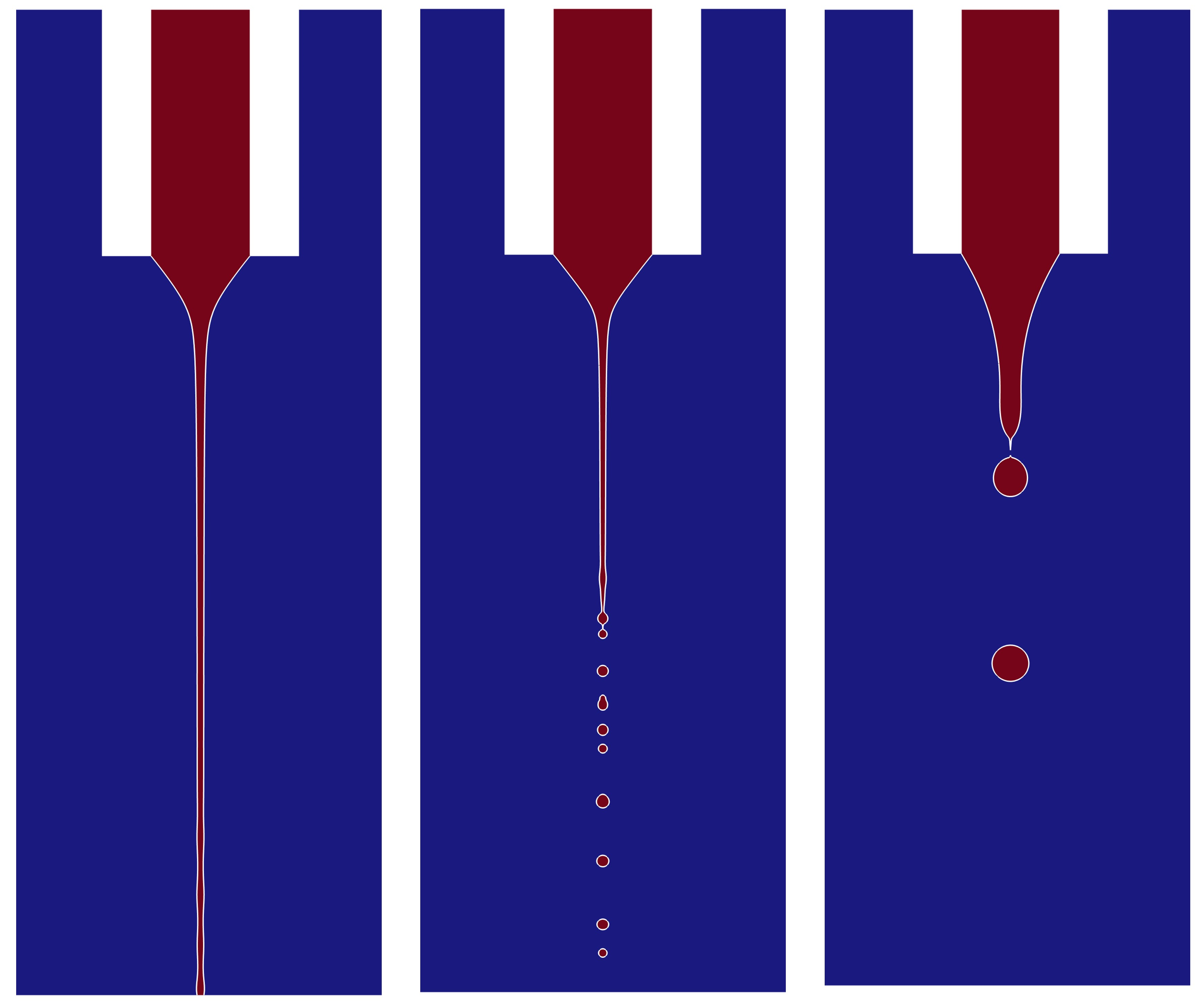
The printing height directly affects whether the jet will break up above the substrate. If the printing height is too low, the jet will not break up no matter what the other parameters are. The influence of the printing height on the printing behaviour and the frequency is studied by changing the printing height while keeping other dimensionless numbers unchanged. In the derivation by Ismail et al. (Reference Ismail, Yao, Xia and Stark2018), the jet breakup length will remain unchanged if the electric field strength is fixed for a certain liquid with a constant flow rate. From figure 8, it can be seen that the z-coordinates of the jet breakup points are almost constant with the increase of the printing height. This finding is consistent with Ismail et al. (Reference Ismail, Yao, Xia and Stark2018) for Ca e is fixed at 4.5 in our study, which is achieved by adjusting V 0 to make E 0 without varying. The jet reaches the substrate when the printing height is low, and has a long distance of droplet flight when the printing height is high. Therefore, the printing height is set as 15R i in the following simulation because the breakup above the substrate can occur and the computational cost is relatively low. On the other hand, the printing frequency decreases first and seems to maintain near 70 kHz. This demonstrates that the low printing height is not conducive to droplets’ formation, but helps to increase the printing frequency. When the printing height is high enough, the impact of continuously increasing the printing height on the printing frequency is negligible.
The printing states at
 $\hat{t}=11$
and frequencies of the EHD printing with different printing height H = 5R
i
, 10R
i
, 15R
i
, 20R
i
, 25R
i
, 30R
i
. The dimensionless numbers here are Oh = 0.05,
 $\alpha$
= 0.5, Ca
e
= 4.5, We = 0.002.

5.3. The influence of liquid’s properties and process parameters on the printing behaviours and frequencies
Since gravity is constant, the Bo is set to be a certain value. The remaining four dimensionless numbers Oh,
 $\alpha$
, We and Ca
e
are used to measure the influence of the liquid’s viscosity, conductivity, printing voltage and the flow rate on the printing behaviours and the frequency. These four parameters are divided into two categories. The liquid’s viscosity and conductivity are two of liquid’s properties. The printing voltage and flow rate are part of the process parameters. The nozzle’s diameter, printing height, surface tension, liquid’s density and relative permittivity remain unchanged.
In order to obtain the frequency of droplet generation, the most important thing to do is to determine under what circumstances droplets will be produced and how they are generated. Starting with the liquid’s properties, the phase diagram of the EHD printing modes in the Oh–
 $\alpha$
space is plotted in figure 9(a). Here, based on the characteristics of the jet pinch-off, the printing modes are categorized into the reaching substrate mode, long jet mode and short jet mode. Just as the names imply, the jet directly reaches the substrate without breaking into droplets in reaching substrate mode. In the long jet and the short jet mode, the jet lengths are ‘long’ and ‘short’, respectively. Obviously from figure 9(a), a large Oh and small
 $\alpha$
will cause the jet to directly contact the substrate. An increasing
 $\alpha$
will lead to a shorter jet length. Therefore, the simultaneous occurrence of large Oh and small
 $\alpha$
should be avoided to ensure that droplets are produced above the substrate.
(a) The Oh-
 $\alpha$
phase diagram of the EHD printing modes, including the reaching substrate, long jet and short jet modes. (b) Three typical cases in different modes.

The jet length is defined as the maximum z-coordinate of the continuous air–liquid interface in contact with the nozzle. Whether the jet length is long or short depends on the comparison with 5R i , which can be seen in figure 9(b). This is for the reason that when the jet length is less than 5R i , the jet breaks up mainly due to so-called end-pinching instability where droplets are generated one by one at the tip of the jet. When the jet length is longer than 5R i , the jet transforms into droplets primarily based on the Rayleigh–Plateau instability. The further explanation for this is that the breakup caused by Rayleigh–Plateau instability needs the growth of the surface disturbance’s amplitude along the jet’s flow. Only a long jet’s length can ensure that the disturbance amplitude increases to a sufficiently large value to make the pinch-off happen. Therefore, the long jet mode is primarily due to Rayleigh–Plateau instability, while the short jet mode is mainly caused by end-pinching instability. In the long jet mode, the chasing and coalescence phenomenon can be observed, as shown in figure 10. This phenomenon leads to a decrease in printing frequency, for two ‘proto-drops’ (Ponce-Torres et al. Reference Ponce-Torres, Rebollo-Muñoz, Herrada, Gañán-Calvo and Montanero2018) coalesce into one droplet.
The chasing and coalescence phenomenon at the jet’s tip in the printing process. Here, Oh = 0.05,
 $\alpha$
= 0.5, Ca
e
= 4.5, We = 0.002.

By changing
 $\alpha$
and Oh, the printing frequency will vary accordingly with relationships in figures 11(a) and 11(b), where all the relationships exhibit a monotonic feature. Figure 11(a) shows that the printing frequencies increase with the decrease of
 $\alpha$
. This is for the reason that as other parameters are constant, the smaller
 $\alpha$
leads to a thinner jet. As the printing flow rate is set at a certain value, more droplets will be produced from the thinner jet in a fixed period of time. This results in a higher printing frequency. As for Oh in figure 11(b), smaller Oh also causes the printing jet to have a smaller diameter, which makes the frequency vary with Oh in the same pattern as changing
 $\alpha$
. The maximum printing frequency here reaches near 55f
c
, revealing the frequency advantage of EHD printing’s droplet mode.
The printing frequencies vary with (a)
 $\alpha$
when Oh = 0.02, 0.03 and 0.05; (b) Oh when
 $\alpha$
= 0.1, 0.5 and 1.0. Here, Ca
e
= 4.5 and We = 0.002.

The variations of
 $\overline{\varDelta _{t}}$
converging with
 $N_{d}$
are also plotted in figures 12(a–c) and 12(d–f). Regardless of whether the
 $\overline{\varDelta _{t}}$
is increasing, decreasing or oscillating with increasing
 $N_{d}$
, it will finally remain relatively stable around a constant value. This demonstrates the reliability of frequency measurement in this work.
The variations of
 $\overline{\varDelta _{t}}$
converging with
 $N_{d}$
when
 $\alpha=0.5$
with Oh = (a) 0.02, (b) 0.03, (c) 0.05 and Oh = 0.04 with
 $\alpha$
= (d) 0.1, (e) 0.5, (f) 1.0. Here, Ca
e
= 4.5 and We = 0.002.

Moreover, the influence of Ca
e
on the printing frequency is studied, which can be seen in figure 13. The cases here have Oh = 0.05,
 $\alpha$
= 5 and We = 0.002. In the case presented here, the droplets are generated due to end-pinching instability when Ca
e
is small, and the droplets’ diameters are relatively large. As a result, the printing frequency is comparatively low. When Ca
e
is increasing, the Rayleigh–Plateau instability plays a more significant role in the jet pinch-off, and the droplets’ diameters become smaller. Therefore, the printing frequency becomes higher with larger Ca
e
. As the longer jet prompts the chasing coalescence phenomena to occur more frequently, the printing frequency is limited to further increase and reaches its maximum. The frequencies of EHD printing based on both short and long jet modes are higher than f
c
and have a maximum of near 3f
c
. More experimental results can be seen in Appendix B, which shows a similar law with the numerical calculations.
The effect of Ca
e
on the printing frequency. The regimes with different colours denote different printing modes, where the red regime represents the short jet mode, and the blue regime indicates the long jet mode. Here, Oh = 0.05,
 $\alpha=5$
and We = 0.002.

Upon careful observation of figures 11(a) and 11(b), it can be found that there might be some scaling relationships between printing frequency and other dimensionless numbers used in this work. Considering the mass conservation and the incompressibility of the liquid, the total volume of the generated droplets per unit time must be the same as the printing flow rate. In the most probable situation, the jet diameter d
j
is 1.89 times that of droplets’ diameters d (Cloupeau & Prunet-Foch Reference Cloupeau and Prunet-Foch1994). This indicates
 $d\sim d_{j}$
. Therefore, the mass conservation equation can be written as follows:
 \begin{align} Q\sim fd^{3}\sim fd_{j}^{3} . \end{align}
The scaling laws for d
j
with respect to different range of
 $\alpha$
have been derived by Gañán–Calvo (Reference Gañán-Calvo2004) and Collins et al. (Reference Collins, Sambath, Harris and Basaran2013),
 \begin{align} d_{j}\sim \begin{cases} \alpha ^{1/6}, \text{smaller}\, \alpha ,\\[3pt] \alpha ^{1/2},\text{larger} \, \alpha . \end{cases} \end{align}
As for the Oh, there is (Gañán-Calvo Reference Gañán-Calvo2004)
 \begin{align} d_{j}\sim Oh^{1/8} . \end{align}
Combining the above formulae and the numerical results, the scaling laws for d j in the case of constant Q are
 \begin{align} f\sim d_{j}^{-3}\sim \begin{cases} \left(\alpha ^{1/6}Oh^{1/8}\right)^{-3}\sim \alpha ^{-1/2}Oh^{-3/8}, \alpha \leq 1,\\[3pt] \left(\alpha ^{1/2}Oh^{1/8}\right)^{-3}\sim \alpha ^{-3/2}Oh^{-3/8}, \alpha \gt 1. \end{cases} \end{align}
By summarizing the simulation data, We can be introduced to (5.5) to obtain the final scaling laws for printing frequency f:
 \begin{align} f\sim \begin{cases} \alpha ^{-1/2}We^{-1/4}Oh^{-3/8}, \alpha \leq 1,\\[3pt] \alpha ^{-3/2}We^{-1/6}Oh^{-3/8}, \alpha \gt 1. \end{cases} \end{align}
From (5.6), the decrease of We causes the increase of the printing frequency. This rule is also discovered by experiments, which can be seen in Appendix B. The reason for this law is that the decrease in We leads to smaller jet diameters and rarer chasing coalescence phenomena. Moreover,
 $\alpha =1$
is the turning point of the scaling laws. This can be explained by the definition in (3.20), where the physical meaning of
 $\alpha$
is the ratio of the charge relaxation time to the capillary time. Here
 $\alpha =1$
is a special situation when the charge relaxation effect and capillary effect are comparable. In this case, the liquid can be considered as leaky-dielectric. When the value of
 $\alpha$
becomes larger or smaller than unity, the liquid is more inclined towards dielectric or conductor. As a result, the competitive relationship between the charge relaxation effect and capillary effect makes
 $\alpha =1$
become the turning point of the obtained scaling laws. The scaling laws are validated using numerical results, as seen in figure 14. This will be helpful for obtaining higher printing frequency using the droplet mode in the EHD printing process.
The scaling laws for printing frequency (a)
 $f\sim \alpha ^{-1/2}We^{-1/4}Oh^{-3/8}$
(solid line) when
 $\alpha \leq 1$
and (b)
 $f\sim \alpha ^{-3/2}We^{-1/6}Oh^{-3/8}$
(solid line) when
 $\alpha \gt 1$
. The coloured symbols denote results from simulations. The dimensionless number Ca
e
= 4.5 in all cases here.

6. Conclusion
This study aims to investigate high-frequency droplet production in EHD printing technology. The high-frequency characteristics of the droplet mode are validated by the experimental method. The characteristic frequency is broken through. The continuous generation of the droplets is calculated by using a numerical model coupled with flow field, electric field, PNP equation and phase field to reveal its mechanism. The unreal charge leakage is prevented by constructing a transition function for liquid’s properties. The parameter independent analysis and the experimental validation are carried out to ensure the accuracy of the simulation. The stability of the Taylor cone’s deformation and the droplets’ generation is studied. The measurement criterion for printing frequency is determined. The influence of the printing height, liquid conductivity, liquid viscosity, flow rate and printing voltage on the printing behaviours and frequencies are explored. The main conclusions can be summarized as follows.
-
(i) The profile and the cone angle of the Taylor cone will gradually converge as time goes by. The average time interval between two consecutive droplets
 $\overline{\varDelta _{t}}$
gradually approaches convergence value with
$N_{d}$
(the number of the generated droplets after the time when
$\varDelta_r$
is just less than 1 %) increasing. This indicates that the printing frequency tends to be stable as more droplets are produced.
-
(ii) The higher printing height makes it easier for the jet to break up into droplets. If the printing height is too low, the jet will always reach the substrate no matter what the other parameters are. The printing frequency decreases first and maintains around a certain value with the increase of the printing height.
-
(iii) A larger Oh and smaller
$\alpha$
will cause the jet length to increase. A large
$\alpha$
will lead to a short jet. The chasing and coalescence phenomenon in the long jet mode limits the increase of the printing frequency. The printing frequency increases with the decrease of
$\alpha$
, Oh, We and the increase of Ca
e
. The scaling laws for printing frequencies can be expressed as
$f\sim \alpha ^{-1/2}We^{-1/4}Oh^{-3/8}$
with
$\alpha \leq 1$
and
$f\sim \alpha ^{-3/2}We^{-1/6}Oh^{-3/8}$
with
$\alpha \gt 1$
.


The comparison of the droplets’ continuous generation between (a) experimental results and (b) the simulations. The scale bar is 100 μm. The droplet here has a diameter of around 32 μm, which corresponds to a volume of 17 pL.

The results obtained are useful for not only obtaining higher printing frequency but also the comprehension of the droplet generation’s mechanism in EHD printing technology. However, the time interval between two consecutive droplets’ production is not stable enough for industrial applications. Further research may focus on the regulation of printing stability to improve the manufacturing capability of EHD printing via the droplet mode. Only then can EHD printing really meet the requirements of the large-scale manufacturing process.
Funding
This work was supported by the CUI CAN Program of Guangdong Province (grant no. CC/XM-202402ZJ0102), the National Natural Science Foundation of China (grant no. 52 205 594) and the Fundamental Research Funds for the Central Universities (HUST: 2025JYCXJJ033).
Declaration of interests
The authors report no conflict of interest.
Appendix A. Validation of the numerical model’s printing frequency
The accuracy of the printing frequency of simulations in this study is verified by simulating the experimental conditions in figure 1(b). The experiments and numerical calculations are shown in figures 15(a) and 15(b), respectively. The images showing the experimental results have the problem of motion blur due to the small size, high generation frequency and fast speed of droplets. This makes the spherical droplets appear to have long tails, which is not real. The comparison in figure 15 shows a good consistency. The printing frequency of the simulations is the same as the experimental frequency, which is 5 kHz. This illustrates the accuracy of the numerical model’s printing frequency.
Appendix B. Experimental results about the influence of back pressure and printing voltage on the printing frequency
The effect of back pressure and printing voltage on the printing frequency is further investigated by the experimental method. The liquid material used here has a very low conductivity, making its
 $\alpha$
larger than unity. The trend of printing frequency varying with printing voltage in figure 16(a) is consistent with what is plotted in figure 13. This trend is not affected by the relationship between Ca
e
and V
0 (
 $Ca_{e}\sim V_{0}^{2}$
from the definition of Ca
e
and E
0). Because the back pressure instead of the flow rate is used in the experiment, the relationship between them can be described by introducing Poiseuille’s law (
 $p\sim Q$
). Figure 16(b) illustrates the scaling law
 $f\sim p^{-1/3}\sim Q^{-1/3}\sim We^{-1/6}$
, which has a good agreement with (5.6).
The experimental results about printing frequency varying with (a) printing voltage when printing height is 15 mm and back pressure is 55 kPa, and (b) back pressure when printing height is 15 mm and printing voltage is 2.6 kV.



