2.1. Flow configuration

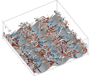
The turbulent oscillatory flow over two-dimensional vortex ripples (illustrated in figure 1) is numerically investigated using DNSs in this study. For the flow configuration, a Cartesian coordinate system is defined on the average plane of the ripple surface, which has a size of $L_1 \times L_2$ in the streamwise and spanwise directions, respectively. In the vertical direction, the physical domain has an average height of $L_3$, from the average bottom to the top boundary. Driven by a vertically uniform oscillatory pressure gradient, the turbulent flow oscillates periodically in the streamwise direction over vortex ripples characterized by their wavelength of $L_{r}$ and height of $h_r$.

Figure 1.

Sketch of the flow domain. Turbulent sinusoidal flow oscillates over a two-dimensional rippled bed with dimensions of $L_{r}$ and $h_r$ corresponding to the ripple wavelength and height, respectively. The attached Cartesian coordinate system is located on the average bottom with the $x_1$-axis in the direction of the fluid oscillation, the $x_2$-axis aligned along the ripple crest and the $x_3$-axis pointing vertically upwards.

For equilibrium vortex ripples, the ripple profile $\eta _r(x_1,x_2)$ is a function of ripple dimensions, i.e. $\eta _r=\eta _r(L_{r},h_r)$. As a result, for a specific ripple profile, there are three essential length scales in the present problem: the wave semi-orbital excursion length $A$, the ripple wavelength $L_{r}$ and the ripple height $h_r$. The time scale in this problem is the wave period $T_w$, where $\varOmega _w=2{\rm \pi} /T_w$ is the corresponding angular frequency. Based on these characteristic length and time scales, the problem of turbulent oscillatory flow over vortex ripples is characterized by three dimensionless parameters (Önder & Yuan Reference Önder and Yuan2019): the Reynolds number

(2.1)\begin{equation} Re=\frac{A^2\varOmega_w}{\nu}, \end{equation}

where $\nu$ is the fluid kinematic viscosity; the Keulegan–Carpenter number

(2.2)\begin{equation} K_C=2{\rm \pi}\frac{A}{L_{r}}, \end{equation}

which describes the ratio between the wave semi-orbital excursion and the ripple wavelength; and the ripple steepness

(2.3)\begin{equation} s=\frac{h_r}{L_{r}}. \end{equation}

For equilibrium orbital ripples, $L_{r}$ is proportional to $A$ such that $K_C$ is approximately $5$. According to field measurements and laboratory experiments, the orbital ripple steepness is approximately $0.17$. The Reynolds number is typically in the range of O $(10^4)$ to O $(10^5)$.

The shape of vortex ripples generated by wave boundary layers could be important in the local hydrodynamics and sediment transport, which is a result of many factors such as the oscillatory flow intensity, wave period, wave nonlinearity, horizontal steady streaming, migration direction and sediment properties (Wang & Yuan Reference Wang and Yuan2019; Sishah & Vittori Reference Sishah and Vittori2022). In order to avoid additional complexity, similar to Önder & Yuan (Reference Önder and Yuan2019), the bottom profile in all our simulations is defined as the superposition of two harmonics, which reads

(2.4)\begin{equation} \eta_r=\frac{h_r}{2}\left(\cos{k_r}{x_1}+a\cos{2k_r}{x_1}\right), \end{equation}

where $k_r=2{\rm \pi} /L_{r}$ is the wavenumber of the ripple waviness, and the relative amplitude of the second harmonic is prescribed to be $a=0.17$ following Önder & Yuan (Reference Önder and Yuan2019). Therefore, we assume a smooth ripple wall in this study while in a realistic situation the sandy bed is rough with active particle movements, and our ripple profile using superposition of two harmonics is still an idealization of complex ripple geometry observed in nature (Du Toit & Sleath Reference Du Toit and Sleath1981; van der Werf et al. Reference van der Werf, Magar, Malarkey, Guizien and O'Donoghue2008).

2.2. Governing equations

Although the wave nonlinearity is important in ripple migration and sediment transport (van der Werf et al. Reference van der Werf, Doucette, O'Donoghue and Ribberink2007; Yuan & Wang Reference Yuan and Wang2019), we focus on a sinusoidally oscillatory viscous flow over a wavy bottom in order to understand how the leading quantities, namely the ripple wavelength and height, are related to the flow characteristics. Tensor notation is used in this study and the subscript $i=1,2,3$ corresponds to the streamwise, spanwise and vertical directions, respectively. The governing equations are the continuity equation and the incompressible Navier–Stokes equations, which respectively read

(2.5)\begin{gather} \frac{\partial u_i}{\partial x_i}=0, \end{gather}

(2.6)\begin{gather}\frac{\partial u_i}{\partial t}+u_j\frac{\partial u_i}{\partial x_j}={-}\frac{1}{\rho}\frac{\partial p}{\partial x_i}+ \frac{1}{\rho}\frac{\partial\tau_{ij}}{\partial x_j}+ F_w\delta_{i1}, \end{gather}

where $u_i$ is the velocity field, $\rho$ is the fluid density, $p$ is the pressure field and $\delta _{ij}$ is the Kronecker delta; ${\tau }_{ij}=2\mu S_{ij}$ is the viscous stress tensor where $\mu$ is the fluid dynamic viscosity and $S_{ij}$ is the strain-rate tensor which reads

(2.7)\begin{equation} S_{ij}=\frac{1}{2}\left(\frac{\partial u_i}{\partial x_j}+\frac{\partial u_j}{\partial x_i}\right). \end{equation}

The last term in (2.6) is the driving force in the streamwise direction, where $F_w$ is a vertically uniform oscillatory pressure gradient in the streamwise direction, reading

(2.8)\begin{equation} F_w=U_w\varOmega_w\sin{\left(\varOmega_w t\right)}=U_w\varOmega_w\sin{\theta}. \end{equation}

The effects of wave skewness (Ribberink & Al-Salem Reference Ribberink and Al-Salem1994) and asymmetry (Elgar et al. Reference Elgar, Guza, Raubenheimer, Herbers and Gallagher1997) are not considered in this study, and the driven flow has a resultant sinusoidal free-stream velocity $u_w=-U_w\cos {\theta }$, where $U_w$ is the free-stream velocity amplitude and $\theta =\varOmega _w t$ is denoted as the wave phase hereafter. Therefore, corresponding to the wave phase $\theta =0$, the free-stream velocity starts from the value of $u_w=-U_w$ and decelerates to the instant of flow reversal. Based on (2.8), the wave semi-orbital excursion length is calculated as $A=U_w/\varOmega _w$.

In our numerical set-up, the physical domain (figure 1) has a shear-free top boundary where the free-slip, rigid-lid boundary condition is implemented, which reads

(2.9)\begin{equation} \frac{\partial u_1}{\partial x_3}=0,\quad \frac{\partial u_2}{\partial x_3}=0,\quad u_3=0,\quad\text{at } x_3=L_3. \end{equation}

In contrast, the bottom of the physical domain is modelled as a fixed bed, and the no-slip boundary condition is applied for the fluid velocities, which is written as

(2.10)\begin{equation} u_i=0,\quad\text{at } x_3=\eta_r. \end{equation}

The oscillatory viscous flow over vortex ripples is treated as a boundary layer flow with periodic boundary conditions implemented in the streamwise and spanwise directions.

2.3. Numerical implementation

A major difficulty in the simulation of the flow over a bedform is that the physical domain has undulatory boundaries (illustrated in figure 1), which cannot be easily discretized using the commonly used regular grid system. To discretize the irregular physical domain, a boundary-fitted grid system in the Cartesian coordinates $(x_i;t)$ is applied in the physical space, as shown in figure 2(a). Then, a new computational coordinate system is introduced by adopting the following algebraic mapping

(2.11)\begin{equation} x_1=\xi_1,\quad x_2=\xi_2,\quad x_3=\left(1-\frac{\eta_r}{L_3}\right)\xi_3+\eta_r,\quad t=\zeta. \end{equation}

With this coordinate transformation, the irregular physical domain is transformed into a rectangular computational domain as shown in figure 2(b). In the computational space, the top and bottom boundaries are represented by $\xi _3=L_3$ and $\xi _3=0$, respectively. Namely, the resulting size of the computational domain is $L_1 \times L_2 \times L_3$.

Figure 2.

Illustration of the coordinate transformation: (a) boundary-fitted grid of the irregular domain in the physical space $(x_i;t)$; (b) mapped grid of the rectangular domain in the computational space $(\xi _i;\zeta )$. Note that the uniform grid is applied in both the $x_2$ and $\xi _2$ directions.

By applying the chain rule of partial derivatives, the governing equations (2.5) and (2.6) are rewritten in terms of the curvilinear coordinates $(\xi _i;\zeta )$ in the computational space (Yang & Shen Reference Yang and Shen2010, Reference Yang and Shen2011). The transformed governing equations are integrated in time by the third-order Runge–Kutta scheme. For spatial discretization, we use the pseudo-spectral method on uniform grids ($N_1 \times N_2$) in the $\xi _1$ and $\xi _2$ directions, along with the Chebyshev collocation method on the Chebyshev–Gauss–Lobatto points ($N_3$) in the $\xi _3$ direction. The open-source code TURBID (https://github.com/yueliangyi/TURBID, Yue, Cheng & Hsu Reference Yue, Cheng and Hsu2019) is upgraded to solve the transformed equations where the numerical schemes are presented in Yue (Reference Yue2020). Figure 3 shows a good agreement of turbulence-averaged quantities between the case kc1.0s1.0 (listed in table 1) and the case C2 in Önder & Yuan (Reference Önder and Yuan2019). This provides validation of our numerical model.

Figure 3.

Vertical profiles of the turbulence-averaged streamwise velocity $\langle u_1\rangle _{p2}/U_w$, vertical velocity $\langle u_3\rangle _{p2}/U_w$, pressure $\langle p\rangle _{p2}/\rho U_w$ and turbulence kinetic energy $\langle e_t\rangle _{p2}/U_w^2$ with $e_t=0.5u_i^\prime u_i^\prime$ at the flow reversal in (a–d) and flow peak in (e–h). Solid lines correspond to the present simulation results while crosses are results of the case C2 discussed in Önder & Yuan (Reference Önder and Yuan2019). Variable values are illustrated using a local blue axis, and variable notions are given in § 2.5.

Table 1.

Physical and computational parameters of the simulations. The reference case kc1.0s1.0 has ripple dimensions of $L_{r0}=6.78\,{\rm cm}$ and $h_{r0}=1.13\,{\rm cm}$, corresponding to the reference parameters $K_{C0}=5.24$ and $s_0=0.17$. Case names are based on the Keulegan–Carpenter number and the ripple steepness for each run compared with the reference case, such that the case kc0.8s1.0 corresponds to the simulation with $K_C=0.8K_{C0}$ and $s=1.0s_0$. The size of the computational domain is selected based on the ripple wavelength of the specific simulation case. Here, $N_T$ is the total run time of simulation in units of wave period.

2.4. Numerical experiments

Numerical simulations with a free-stream velocity amplitude of $U_w=4.42\,{\rm cm}\,{\rm s}^{-1}$ and $T_w=8.02\,{\rm s}$ are carried out in this study. This wave condition results in an angular frequency of $\varOmega _w=0.78\,{\rm s}^{-1}$ and a wave semi-orbital excursion of $A=U_w/\varOmega _w=5.65\,{\rm cm}$. Four cases (listed in table 1) are designed to study the effect of different ripple dimensions on the resulting fluid kinematics and dynamics, thus revealing the mechanism in the selection of orbital ripple dimensions. In case kc1.0s1.0, the ripple bed is regarded to be in equilibrium with dimensions of $L_{r0}=6.78\,{\rm cm}$ and $h_{r0}=1.13\,{\rm cm}$, resulting in the reference parameters of $K_{C0}=5.24$ and $s_0=0.17$. These reference parameters are consistent with most empirical formulas (Pedocchi & García Reference Pedocchi and García2009; Nelson et al. Reference Nelson, Voulgaris and Traykovski2013; Wang & Yuan Reference Wang and Yuan2019) for predicting equilibrium vortex ripple dimensions. The other three cases are taken with different ripple dimensions but keep the same $K_C$ or $s$ as the case kc1.0s1.0. By increasing the ripple length by $20\,\%$ in case kc0.8s1.0, reducing the ripple length by $20\,\%$ in case kc1.2s1.0 or decreasing ripple steepness by $10\,\%$ in case kc1.0s0.9, we can investigate the adequate change in vortex intensity characterizing the turbulent oscillatory flow in an idealized domain. The resulting Reynolds number for all cases is only $Re=2500$, which is one order smaller than the value in laboratory experiments or field measurements. However, this does not defeat the main objective of this study, which is to reveal the fundamental kinematic characteristics of oscillatory flows over ripples with different dimensions using an idealized model. As shown in table 1, for all four cases, $K_C$ has a range of $4.19$ to $6.29$, while $s$ has a range of $0.15$ to $0.17$. Thus, a moderate range of parameters is investigated in this study.

For all numerical simulations presented in this study, the size of the computational domain is chosen based on the ripple wavelength of a specific simulation case. The same criterion is used by Önder & Yuan (Reference Önder and Yuan2019). The computational domain is confirmed to be large enough by computing the two-point correlation functions. This can also be inferred by the analysis of the computational domain size in appendix B of Önder & Yuan (Reference Önder and Yuan2019). In all cases, the flow is initialized with appropriate divergence-free sinusoidal perturbations at the flow reversal. Data sampling starts from $t=6T_w$, when the flow is observed to reach a quasi-steady state, to the end of the simulation ($t=N_TT_w$). The number of grid points for each case simulated in this study is also listed in table 1. The spatial resolutions are assessed in the wall units denoted by a superscript ‘$+$’, where the grid spacing is non-dimensionalized by the viscous length scale $\nu /u_\tau$. The local friction velocity is calculated as $u_\tau =\sqrt {\langle {\tau _{w1}}\rangle _{p}/\rho }$, where $\langle {\tau _{w1}}\rangle _{p}$ is the streamwise component of the phase-averaged shear stress on the ripple surface (defined in § 3.4). The grid assessment is shown in figure 4, where a grid resolution of $\Delta x_1^+\leq 13.8$ and $\Delta x_2^+\leq 9.2$ is found in the streamwise and spanwise directions. In the vertical direction, we obtain $\Delta x_3^+\leq 0.19$ close to the wall and $\Delta x_3^+\leq 15.3$ in the middle of the water column. This grid resolution is similar to the one used in Ozdemir, Hsu & Balachandar (Reference Ozdemir, Hsu and Balachandar2010) for studying the turbulent oscillatory flow over a flat wall. Especially for the case kc0.8s1.0, the grid resolution is even finer due to more intense turbulence.

Figure 4.

Grid resolution in wall units over a half-flow cycle: (a,b) maximum grid spacings in the streamwise and spanwise directions, respectively; (c) maximum and (d) minimum grid spacings in the vertical direction.

2.5. Variable decomposition and notation

The phase-average approach (Reynolds & Hussain Reference Reynolds and Hussain1972) has been widely used to quantify the modulation of statistical properties of turbulence by the underlying wave motion (Nelson & Fringer Reference Nelson and Fringer2018; Yue, Cheng & Hsu Reference Yue, Cheng and Hsu2020). The phase averaging of an arbitrary variable $\psi$ in a quasi-steady state is defined as

(2.12)\begin{equation} \langle\psi\rangle_{p}=\frac{1}{N_w}\sum_{n=1}^{N_w}\psi\left(x_1,x_2,x_3;t+nT_w\right) ,\quad\text{for } 0\le t< T_w, \end{equation}

where the symbol $\langle \;\rangle$ denotes the operation of averaging, and $N_w$ is the number of wave periods during which the averaging is taken. The time averaging of $\psi$ is defined as

(2.13)\begin{equation} \bar{\psi}=\frac{1}{N_wT_w}\int_{0}^{N_wT_w}\psi\left(x_1,x_2,x_3;t\right)\,\mathrm{d}t. \end{equation}

Note that $t=\zeta$ in the coordinate transformation (2.11), such that the defined time and phase averaging is also applicable in the transformed domain, i.e. figure 2(b). In addition to the averaging over time, spatial averaging in the transformed domain reads

(2.14)\begin{equation} \langle\psi\rangle_{i}=\frac{1}{L_i}\int_{0}^{L_i}\psi\left(\xi_1,\xi_2,\xi_3;\zeta\right)\,\mathrm{d}\xi_i, \end{equation}

where the subscript $i$ ($i=1$, $2$ or $3$) of the average operator $\langle \;\rangle$ denotes a spatial averaging in the corresponding direction.

In this study, the bedform is two-dimensional and the flow is regarded to be homogeneous in the spanwise direction. Consequently, the turbulence-averaging operator $\langle \;\rangle _{p2}$, implying the phase and $\xi _2$ averaging, is used to separate the turbulence fluctuation. With the defined turbulence averaging, the variable $\psi$ is decomposed as $\psi =\langle \psi \rangle _{p2}+\psi ^\prime$, where $\psi ^\prime$ is the corresponding turbulent fluctuation component. Furthermore, for the statistically steady turbulent flow over a bedform, the turbulence-averaged quantity can be further decomposed using a spatial (streamwise) averaging (Hara & Sullivan Reference Hara and Sullivan2015), leading to a triple decomposition of the variable $\psi$ as

(2.15)\begin{equation} \psi = \langle\psi\rangle_{w}\left(\xi_3;\zeta\right)+\langle\psi\rangle_{r}\left(\xi_1,\xi_3;\zeta\right)+\psi^\prime\left(\xi_1,\xi_2,\xi_3;\zeta\right), \end{equation}

where $\langle \psi \rangle _{p2}=\langle \psi \rangle _{w}+\langle \psi \rangle _{r}$. The term $\langle \psi \rangle _{w}=\langle \psi \rangle _{p12}$ is the ripple-averaged but time-dependent mean flow. Due to its time dependency under wave motion, it is called the ripple-averaged wave-induced motion in this study. Accordingly, the term $\langle \psi \rangle _{r}=\langle \psi \rangle _{p2}-\langle \psi \rangle _{w}$ is denoted as the ripple-induced fluctuation. Note that, the phase-, time- and spatial-average operations correspondingly defined in (2.12) to (2.14) are commutative. The triple decomposition defined in (2.15) is applied to the instantaneous velocity profile $u_1$ at flow peak (crest) in the oscillatory flow (see figure 5). The component of ripple-averaged wave-induced motion contains the background velocity with a relatively uniform distribution far from the rippled bed (figure 5b). Organized spatial variation in the velocity field $u_1$ (e.g. vortices) is contained in the ripple-induced fluctuation, which has higher intensity close to the ripple surface (figure 5c). The random flow structure is found in the turbulent fluctuation (figure 5d). Similar triple decomposition approaches have been widely used in previous works (Sullivan, Mcwilliams & Moeng Reference Sullivan, Mcwilliams and Moeng2000; Yang & Shen Reference Yang and Shen2010; Buckley & Veron Reference Buckley and Veron2019; Zhang, Huang & Xu Reference Zhang, Huang and Xu2019).

Figure 5.

Illustration of the triple decomposition of the streamwise velocity: (a) instantaneous velocity profile $u_1$ at a flow peak; (b) the ripple-averaged wave-induced motion $\langle u_1\rangle _{w}$; (c) the ripple-induced fluctuation $\langle u_1\rangle _{r}$; (d) the turbulent fluctuation $u_1^\prime$. All the velocities are normalized by the free-stream velocity amplitude $U_w$.

3.1. Vortex evolution in turbulence-averaged flow

The kinematics of turbulence-averaged flow over ripples are presented in this section, with a special emphasis on the motion of spanwise coherent vortices. To this end, the spanwise vorticity is calculated from the turbulence-averaged velocities as

(3.1)\begin{equation} \langle\omega_2\rangle_{p2} = \frac{\partial\langle u_3\rangle_{p2}}{\partial x_1}- \frac{\partial\langle u_1\rangle_{p2}}{\partial x_3}. \end{equation}

However, the criterion of vorticity cannot always give a satisfactory identification of the region with strong swirling motions if the ambient shear is also strong. For clear identification of vortices, an improved vortex identification method is needed. Alternatively, defined as a measure of local twisting rate within a vortex, the swirling strength criterion proposed by Zhou et al. (Reference Zhou, Adrian, Balachandar and Kendall1999) has been widely used in measured flow fields over rippled beds (Nichols & Foster Reference Nichols and Foster2007; Rodríguez-Abudo & Foster Reference Rodríguez-Abudo and Foster2014; Yuan & Wang Reference Yuan and Wang2019). Although the method of swirling strength can better identify vortices compared with the vorticity, the criterion is still prone to severe contamination by the strong background shearing (Gao & Liu Reference Gao and Liu2018), which is universal in a bottom boundary layer flow. In this study, we adopt a new vortex identification method using the vortex vector (Tian et al. Reference Tian, Gao, Dong and Liu2018, Reference Tian, Fu, Xia and Yang2020) to differentiate the vortices from the background shear flow. The vortex vector is defined based on the local rotation of fluid elements, thus it can exclude the ambient shearing contamination and accurately quantify the local rotational strength. A vortex vector at a point is a vector quantity representing the local fluid rotation and it is defined as

(3.2)\begin{equation} \boldsymbol{R}=2\omega_{rot}\boldsymbol{r}, \end{equation}

where $\boldsymbol {r}$ is the normalized direction of the local fluid-rotation axis which is calculated as the unit eigenvector corresponding to the real eigenvalue of the velocity gradient tensor $\partial u_i/\partial x_j$, and $\omega _{rot}$ is the local fluid-rotational angular velocity, which reads

(3.3)\begin{equation} \omega_{rot}= \begin{cases} \beta-\alpha, & \text{if }\beta>0\text{ and }\alpha^2<\beta^2, \\ \beta+\alpha, & \text{if }\beta<0\text{ and }\alpha^2<\beta^2, \\ 0, & \text{if }\alpha^2\ge\beta^2. \end{cases} \end{equation}

In (3.3), the parameters $\alpha$ and $\beta$, defined as

(3.4)\begin{gather} \alpha= \frac{1}{2}\sqrt{ \left(\frac{\partial V_2}{\partial X_2}-\frac{\partial V_1}{\partial X_1}\right)^2+ \left(\frac{\partial V_2}{\partial X_1}+\frac{\partial V_1}{\partial X_2}\right)^2 }, \end{gather}

(3.5)\begin{gather}\beta= \frac{1}{2}\left(\frac{\partial V_2}{\partial X_1}-\frac{\partial V_1}{\partial X_2}\right), \end{gather}

are calculated from the velocity vector $\boldsymbol {V}$ defined in a local reference frame $\boldsymbol {X}$, where the $X_3$-axis is parallel to $\boldsymbol {r}$, ${\partial V_1}/{\partial X_3}=0$ and ${\partial V_2}/{\partial X_3}=0$. Based on (3.2) to (3.5), a vortex is then defined as a connected region where $\boldsymbol {R}\neq \boldsymbol {0}$, and the iso-surface of the magnitude of vortex vector $|\boldsymbol {R}|$ (denoted as the vortex strength hereafter) can distinctly represent the core of a vortex (Tian et al. Reference Tian, Gao, Dong and Liu2018).

Evolution of the turbulence-averaged velocity and the spanwise vorticity fields throughout the first half-cycle of a wave period is illustrated in figure 6, from the wave phase just after the maximum negative free-stream velocity (a) $\theta =16{\rm \pi} /96$ to the wave phase at the maximum positive free-stream velocity (f) $\theta =96{\rm \pi} /96$. For a better presentation, a local ripple coordinate $\check {x}_1=x_1-x_{1c}$ is employed with $x_{1c}$ being the streamwise location of a ripple crest, such that the ripple crest is always located at $\check {x}_1=0$ and the sign of $\check {x}$ differentiates the two ripple flanks. Due to the periodicity of results in the streamwise direction, the field of view is presented as one ripple wavelength. Although the four cases shown in figure 6 have very different ripple dimensions (see table 1), most of the interesting fluid kinematics happen close to the ripple surface, and we focus on a region from the ripple trough to the specific height of $4h_{r0}$ in the vertical direction.

Figure 6.

Evolution of the turbulence-averaged velocity and the spanwise vorticity fields throughout the half-cycle of a wave period, from the wave phase (a) $\theta =16{\rm \pi} /96$ to (f) $\theta =96{\rm \pi} /96$. The normalized turbulence-averaged velocities $(\langle {u_1}\rangle _{p2},\langle {u_3}\rangle _{p2})/U_w$ are presented as a vector field denoted by the grey arrows, while the corresponding normalized spanwise vorticity $\langle \omega _2\rangle _{p2}/(U_w/L_{r0})$ is presented as iso-surfaces. The coherent vortices are identified using the vortex vector method as the purple contour lines, where the normalized vortex strength criterion of $\langle {|\boldsymbol {R}|}\rangle _{p2}/(U_w/L_{r0})=3$ is implemented. A local ripple coordinate $\check {x}_1=x_1-x_{1c}$ is employed with $x_{1c}$ being the streamwise location of a ripple crest.

In each plot of figure 6, the turbulence-averaged velocities $(\langle {u_1}\rangle _{p2},\langle {u_3}\rangle _{p2})$ are presented by a vector field. Shown as the grey arrows, the evolution of the ambient flow is identified in a region far from the ripple bed, while the modulation of flow caused by the coherent vortices can be clearly observed in a region close to the rippled bed with a notable enhancement in the velocity magnitude. Using the turbulence-averaged velocity field, the corresponding spanwise vorticity $\langle \omega _2\rangle _{p2}$ is calculated following the (3.1) and presented as the iso-surfaces in figure 6. Illustrated by the change of colours of the vorticity iso-surfaces for each simulation, vortices form at the previous accelerating phase before the flow reversal (when $\theta =0$) continues to absorb the flow energy in the deceleration phase between $0<\theta \le {\rm \pi}/2$ (figure 6a–c). During this stage, a primary vortex in the lee ripple flank with $\check {x}_1<0$ can be clearly identified as a closed region with a high positive spanwise vorticity. In the acceleration stage in the interval ${\rm \pi} /2<\theta \le {\rm \pi}$ (figure 6d–f), the coherent vortices separate from the ripple crest, travel large distances with their self-induced velocities, and produce positive jet-like flows as they pass the ripple crest. Meanwhile, the strength of the spanwise (positive) vorticity owned by the ejected primary vortex drops continually to nearly zero. The primary vortex eventually disappears due to the viscous effects. Therefore, the deceleration and acceleration phases are respectively denoted as the vortex-formation and jet-ejection stages in Önder & Yuan (Reference Önder and Yuan2019).

In addition to the high spanwise vorticity, the coherent vortices are identified using the vortex vector method. For each wave phase, the vortex strength field $\langle {|\boldsymbol {R}|}\rangle _{p2}$ is calculated from the corresponding turbulence-averaged flow. The normalized vortex strength criterion of $\langle {|\boldsymbol {R}|}\rangle _{p2}/(U_w/L_{r0})=3$ has been used, which are plotted as the purple contour lines in figure 6. With the threshold of vortex strength used here, vortices are nicely outlined as circles or ellipses over the ripple bed. At most wave phases, more than one vortex has been clearly detected among which there is a primary vortex usually associated with strong spanwise vorticity. In addition to the primary vortex, a secondary or even tertiary vortex around the primary one and near the ripple surface is also detected. The evolution of primary vortices is identified by the size of these iso-lines through different wave phases. For each simulation, during the vortex-formation stage (figure 6a–c), the area circled by the iso-line is growing and hence the newly born primary vortex is developing into larger size and absorbing more energy. During the wave phases (figure 6d–e) when the ejection of the primary vortex is observed, there is no noticeable change in the primary vortex size, and in fact, the turbulence-averaged spanwise vorticity in the primary vortex starts to decay. In the late stage of jet-ejection (figure 6e–f), similar to the spanwise vorticity, the primary vortex size and the intensity are diminishing until its disappearance.

The significance of flow velocity associated with the ripple-induced fluctuation ($\langle u_i\rangle _{r}$, see definition in (2.15)) is also investigated. Similar to the turbulence-averaged spanwise vorticity defined in (3.1), the vorticity carried by the ripple-induced velocity fluctuation is calculated as

(3.6)\begin{equation} \langle\omega_2\rangle_{r}=\frac{\partial\langle u_3\rangle_{r}}{\partial x_1}-\frac{\partial\langle u_1\rangle_{r}}{\partial x_3}. \end{equation}

Evolution of the ripple-induced velocity fluctuation and the corresponding spanwise vorticity fields throughout the first half-cycle of a wave period is shown in figure 7. It is straightforward to find that large velocities are associated with strong vorticity $\langle \omega _2\rangle _{r}$ in figure 7. Compared with the turbulence-averaged velocities in figure 6, there is no phase-dependent background velocity field in the ripple-induced fluctuation. Same as before, coherent vortices can be clearly identified in the ripple-induced fluctuation velocity using the normalized vortex strength with a criterion of $\langle {|\boldsymbol {R}|}\rangle _{p2}/(U_w/L_{r0})=3$. To facilitate the comparison, the coherent vortices detected from the velocity field of turbulence-averaged flow and that of ripple-induced fluctuation are both shown as the purple and green iso-lines in figure 7, respectively. From the close overlapping between these iso-lines, it is clear that the ripple-induced fluctuation carries almost entirely these coherent vortices and the ripple-averaged wave-induced motion is of negligible importance.

Figure 7.

Evolution of the turbulence-averaged velocity and spanwise vorticity fields in the ripple-induced fluctuation throughout the half-cycle of a wave period, from the wave phase (a) $\theta =16{\rm \pi} /96$ to (f) $\theta =96{\rm \pi} /96$. The normalized turbulence-averaged velocities $(\langle {u_1}\rangle _{r},\langle {u_3}\rangle _{r})/U_w$ are presented as a vector field denoted by the grey arrows, while the corresponding normalized spanwise vorticity $\langle \omega _2\rangle _{r}/(U_w/L_{r0})$ is presented as the iso-surface. The coherent vortices are identified in the turbulence-averaged flow and the ripple-induced fluctuation with the criterion of normalized vortex strength $\langle {|\boldsymbol {R}|}\rangle _{p2}/(U_w/L_{r0})=3$, which are respectively shown as the purple and green iso-lines. The local ripple coordinate $\check {x}_1$ is employed.

One of the significant results that distinguishes the coherent vortices over different ripple dimensions is their different strengths (studied in § 3.2) and trajectories. In figure 6, the difference in trajectories of the primary vortices are evident and for comparison, the results are shown here by normalizing the horizontal trajectory with respect to the individual ripple wavelength of each case. In case kc0.8s1.0 where the ripple wavelength is larger than the equilibrium ripple case kc1.0s1.0, the primary vortex first formed at a location relatively close to the ripple crest during the vortex-formation stage (see $\theta =16{\rm \pi} /96$ shown in figure 6c); the vortex centre is located at $\check {x}_1/L_r=-0.25$ for kc0.8s1.0 comparing with $\check {x}_1/L_r=-0.35$ for kc1.0s1.0). Interestingly, the formed lee primary vortex in case kc0.8s1.0 also cannot travel as far away downstream as the equilibrium ripple case kc1.0s1.0 during the jet-ejection stage (see figure 6(e), the vortex centre is located at $\check {x}_1/L_r=0.3$ for kc0.8s1.0 comparing with $\check {x}_1/L_r=0.4$ for kc1.0s1.0). The exact opposite in vortex trajectory can be observed in case kc1.2s1.0 where the ripple wavelength is shorter than the equilibrium value. A similar finding is reported in an experiment by increasing the orbital excursion length (Hare et al. Reference Hare, Hay, Zedel and Cheel2014). By reducing the ripple height, the centre of the primary vortex during its formation shifts towards the ripple crest slightly (see figure 6b). After the ejection of primary vortex from the ripple crest, figure 6 also shows that the small reduction of ripple height does not affect notably on how much distance a primary vortex can travel.

Motivated by these observations, the trajectory of the primary vortex is quantified by its weighted centre $(x_{w1},x_{w3})$, which is defined as

(3.7)\begin{equation} x_{wi}= \frac{\displaystyle\int_{0}^{L_r}\int_{\eta_r}^{L_3}wx_i\,\mathrm{d}\kern0.7pt x_1\,\mathrm{d}\kern0.7pt x_3}{\displaystyle\int_{0}^{L_r}\int_{\eta_r}^{L_3}w\,\mathrm{d}\kern0.7pt x_1\,\mathrm{d}\kern0.7pt x_3}, \end{equation}

where the subscript $i=1$ or $3$. The weight function $w=\langle {|\boldsymbol {R}|}\rangle _{p2}$, when a position is found to be inside or on the primary vortex. Otherwise, $w$ is set to zero. Using the weighted centre, trajectories of the primary vortex for the four cases are presented in both the physical (figure 8a) and transformed (figure 8b) domains. Since the case kc0.8s1.0 has the largest ripple height as $h_{r}=1.25h_{r0}$, the primary vortex travels along a higher trajectory in the physical domain. However, this feature disappears in the transformed domain. Figure 8(b) shows that the parameter $K_C$ does not affect the trajectory of primary vortex evidently in regard to its height for the early and intermediate stages of the vortex evolution. It is only approaching the late stage of vortex evolution that the primary vortex in case kc1.0s1.0 shows the highest trajectory. On the contrary, both in the physical and transformed domain, the height of the primary vortex trajectory shows a clear dependence on the ripple steepness parameter $s$. For the case kc1.0s0.9 with a smaller ripple steepness, the trajectory is closer to the ripple surface. The distance a primary vortex can travel in the streamwise direction during the vortex-formation stage is also observed in figure 8. Generally, the primary vortex can travel relatively farther downstream towards the ripple trough and beyond (where $x_1/L_r<1$) for $K_C$ greater than $K_{C0}$ and its dependence on the ripple steepness is weak. Circles in figure 8 correspond to the first peak in the form drag bottom shear stress shown in figure 11(c), which will be discussed later. Beyond these marked normalized positions, the primary vortices are about to be ejected from the ripple crest into the water column (figure 12c,d). During the vortex-ejection stage, the trajectories in the transformed domain are elevated even though they look flat in the physical domain (figure 8a). Overall, from its generation to full dissipation, the primary vortex is close to the rippled bed in a region below $x_3=4h_{r0}$ (see figure 6). This confirms our finding from figure 6.

Figure 8.

Weighted centre trajectories of primary vortex during the first half-wave cycle: (a) trajectories in the physical domain denoted as thick solid lines; (b) trajectories in the transformed domain. Thin lines in (a) are the ripple profiles for the four numerical cases. Vertical and horizontal coordinates are respectively normalized by $h_{r0}$ and $L_{r}$ for a better comparison. Circles correspond to the group ➀ in figure 11(c), which locates the normalized position of vortex ejection into the water column. Results of one ripple are presented for illustration.

3.2. Time-averaged vortex influence zone

Illustrated in §§ 3.1, a coherent vortex in the turbulence-averaged field dominates the near-bed kinematics of overlying flow. After time averaging, the result of columnar coherent vortices in the carrying flow is illustrated by time-averaged circulation and the corresponding spanwise vorticity (see figure 9). In the figure, the time-averaged velocities $(\langle {\overline {u_1}}\rangle _{2},\langle {\overline {u_3}}\rangle _{2})$ are presented as a vector field and denoted as the grey arrows. Two counter-rotating mean circulations are observed, where the time-averaged spanwise vorticity $\langle {\overline {\omega _2}}\rangle _{2}$, presented as iso-surfaces, has the opposite direction (see red and blue colours). The two circulations are respectively located above the two ripple flanks, centred at the same height with respect to the ripple crest due to the present simple harmonic flow and symmetric ripple profile. They produce a strong mean velocity close to the ripple surface, which conveys water toward the ripple crest. If sediment particles were present, this flow pattern would drive particle fluxes toward the ripple crest and hence maintains the ripple shape. Thus, the two circulations are highly related to the formation mechanism of vortex ripples (Charru, Andreotti & Claudin Reference Charru, Andreotti and Claudin2013). Due to the symmetry of oscillatory flow and ripple profile, the two circulations are equal in strength. A similar observation was obtained in laboratory experiments by, for example, Yuan & Wang (Reference Yuan and Wang2019) and they further demonstrate that if the symmetry is altered, the flow pattern and ripple profile must adjust toward another equilibrium and possibly migrate. Specifically, when the size of circulation zone is smaller than the distance between the adjacent ripples, the circulation can erode the ripple flank and drive the splitting of ripples. On the contrary, when the size of the circulation zone is too large, the vortices tend to carry more particles from the ripple crest and deposit them toward the trough and cause the merging of ripples (Salimi-Tarazouj et al. Reference Salimi-Tarazouj, Hsu, Traykovski and Chauchat2021). Therefore, it is of fundamental importance to relate the circulation pattern to ripple dimensions.

Figure 9.

Time- and $\xi _2$-averaged velocity and vorticity fields. The normalized time-averaged velocities $(\langle {\overline {u_1}}\rangle _{2},\langle {\overline {u_3}}\rangle _{2})/U_w$ are presented as a vector field denoted by the grey arrows, while the corresponding normalized spanwise vorticity $\langle {\overline {\omega _2}}\rangle _{2}/(U_w/L_{r0})$ is presented as iso-surfaces. Purple contour lines denote the normalized strength of the time-averaged vortex vector field (shown in figure 10) where the criterion $|\langle {\bar {\boldsymbol {R}}}\rangle _{2}|/(U_w/L_{r0})=1.5$ is implemented. Results of two ripples are presented for illustration.

Figure 10.

Strength of the time-averaged vortex vector filed $\langle {|\bar {\boldsymbol {R}}|}\rangle _{2}$ after the normalization by $U_w/L_{r0}$. The purple contour lines correspond to the criterion $\langle {|\bar {\boldsymbol {R}}|}\rangle _{2}/(U_w/L_{r0})=1.5$. The black solid circle marks the location of weighted centre. Results of two ripples are presented for illustration.

The strength of these two circulations is quantified by a flux of vorticity, which is defined as the integral of the spanwise vorticity magnitude through the $x_1$–$x_3$ section of the physical domain, written as

(3.8)\begin{equation} \varGamma_2=\int_{0}^{L_r}\int_{\eta_r}^{L_3}\langle{|\overline{\omega_2}|}\rangle_{2}\,\mathrm{d}\kern0.7pt x_1\,\mathrm{d}\kern0.7pt x_3. \end{equation}

Table 2 presents the computed $\varGamma _2$ for the four cases investigated here where $\varGamma _2=0.9389$ $U_wL_{r0}$ in case kc0.8s1.0 is found to be the largest. This indicates that the case kc0.8s1.0 has a relatively strong time-averaged circulation, illustrated by the relatively large velocity around the ripple crests in figure 9(a). The case kc1.2s1.0 has the smallest strength of circulation as $\varGamma _2=0.6143$ $U_wL_{r0}$ which could be significantly suppressed by the short ripple wavelength (figure 9b). As the case kc0.8s1.0 has the largest ripple wavelength (the smallest value of $K_C$) and thus the longest integration length in (3.8), it is more reasonable to quantify the circulation strength with non-dimensional values. When $\varGamma _2$ is normalized by the corresponding ripple wavelength $L_{r}$ for each case, indicating the strength of circulation per unit area (see table 3), it is clear that the case kc1.0s1.0 has the strongest normalized circulation of $0.8054$ $U_w$. The analysis shown here suggests that variation in ripple wavelength away from the equilibrium value reduces the strength of time-averaged normalized circulations. In other words, the equilibrium ripple wavelength corresponds to the maximum of time-averaged normalized circulation. Another important finding from figure 9 is that each of the four cases has different time-averaged influence regions. Indicated by the area occupied by the strong time-averaged spanwise vorticity, there are two influence regions for each ripple crest just above the left and right ripple flanks. In case kc0.8s1.0, when compared with case kc1.0s1.0, the influence regions between two ripple crests are relatively further apart, while they are closer in case kc1.2s1.0. Reducing ripple height also slightly increases the distance between the influence regions (figure 9d) while reducing the strength of circulation compared with the equilibrium case (see tables 2 and 3).

Table 2.

Indices resulting from fluid dynamical controls without spatial averaging over one ripple wavelength.

Table 3.

Indices resulting from fluid dynamical controls after spatial averaging over one ripple wavelength.

The idea of a vortex influence zone is similar to the influence region defined based on the time-averaged spanwise vorticity, which is introduced by Wang & Yuan (Reference Wang and Yuan2018) to explain the asymmetry in ripple profiles caused by gently sloping bottoms. To better quantify the vortex influence zone, we take the strength of the time-averaged vortex vector field $\langle {|\bar {\boldsymbol {R}}|}\rangle _{2}$ as the key parameter, which is shown in figure 10. The purple iso-lines shown in figure 9 correspond to the criterion $\langle {|\bar {\boldsymbol {R}}|}\rangle _{2}/(U_w/L_{r0})=1.5$. Intuitively, both figure 9 and figure 10 illustrate the influence region caused by the evolution of coherent vortices. Comparing these two figures, the strong time-averaged spanwise vorticity is roughly located inside the iso-lines of $\langle {|\bar {\boldsymbol {R}}|}\rangle _{2}/(U_w/L_{r0})=1.5$. However, the field $\langle {|\bar {\boldsymbol {R}}|}\rangle _{2}$ concentrates in a region over the ripple trough, from which the boundary of vortex influence can be more clearly differentiated. Following (3.7), locations of the weighted centre of the iso-lines are also calculated. Based on these weighted centres, the distance between two adjacent centres around one ripple crest is defined as $L_{c}$ and illustrated in figure 10(a), which measures the width of the coherent vortex influence zone (see table 2). In case kc1.0s1.0, where the ripple dimensions are in equilibrium, the distance $L_{c}=0.7144$ $L_{r0}$. When increasing the ripple wavelength by $25\,\%$ while keeping the same ripple steepness in case kc0.8s1.0, we observe $L_{c}=0.7185$ $L_{r0}$ and the increase in $L_{c}$ is negligible even though the coherent vortex has more space to evolve. This means that there exists a maximum width of influence zone for a specific ripple steepness (compare with $L_r=0.6853$ $L_{r0}$ for case kc1.0S0.9). Interestingly, a notably smaller value of $L_{c}=0.6514$ $L_{r0}$ is observed in case kc1.2s1.0 with a reduced ripple wavelength, where the primary vortex that was shed from the ripple crest can reach a location beyond the ripple trough towards the adjacent ripple crest (figures 6b and 8). This leads to cancellation in the time-averaged vortex vector field and is presented as a ‘confliction’ in the field of $\langle {|\bar {\boldsymbol {R}}|}\rangle _{2}$, which can lead to merging of ripples, as mentioned earlier. As mentioned before, by reducing the ripple height in case kc1.0s0.9, a smaller value of $L_{c}=0.6853$ $L_{r0}$ is found, meaning that the ripple height limits how far the vortex separation can reach. Consequently, smaller ripple steepness results in small ripple length as seen in the sub-orbital ripples (Wiberg & Harris Reference Wiberg and Harris1994; Pedocchi & García Reference Pedocchi and García2009). The corresponding normalized distance $L_{c}/L_{r}$ is listed in table 3, where the value of $L_c/L_{r}=0.7817$ in case kc1.2s1.0 is recognized to be the largest, indicating a possible strong interference in the flow over two neighbour ripples.

In addition to the vorticity flux defined in (3.8) based on the time-averaged spanwise vorticity, we further calculate the vortex strength flux using $\langle {\overline {|\boldsymbol {R}|}}\rangle _{2}$ since it is effective in quantifying the averaged strength of vortices generated over the ripples. Defined as the integration of time-averaged vortex strength, the vortex strength flux is written as

(3.9)\begin{equation} \varGamma_v=\int_{0}^{L_r}\int_{\eta_r}^{L_3}\langle{\overline{|\boldsymbol{R}|}}\rangle_{2}\,\mathrm{d}\kern0.7pt x_1\,\mathrm{d}\kern0.7pt x_3. \end{equation}

Listed in table 2, the case kc1.0s1.0 is found to have the maximum vortex strength flux as $\varGamma _v=0.2461$ $U_wL_{r0}$ among the four cases investigated. Even after averaging over one ripple wavelength, the vortex strength flux per ripple wavelength (listed in table 2) in case kc1.0s1.0 remains the largest. Simulation results clearly show that the equilibrium ripple wavelength exists to cause the strongest vortex motion driven by oscillating overlying fluid. Through the comparison between cases with the same ripple wavelength (kc1.0s1.0 and kc1.0s0.9), results also confirm that the larger ripple height results in stronger vortex motion. This finding also supports the conclusion reported by the field measurement (Nichols & Foster Reference Nichols and Foster2007). Note that the Keulegan–Carpenter number in Nichols & Foster (Reference Nichols and Foster2007) is defined based on the ripple height rather than the ripple wavelength. However, for orbital ripples, the ripple steepness is a constant, and the Keulegan–Carpenter number defined using either ripple wavelength and ripple height gives the same conclusion. For cases with the same ripple steepness but different ripple wavelengths (kc0.8s1.0, kc1.0s1.0 and kc1.2s1.0), it is found that $\varGamma _v$ and averaged $\varGamma _v$ per ripple wavelength are largest when the parameter $K_C$ is around the value of $K_{C0}$. For a specific ripple steepness, our results suggest that there exists an optimized condition in ripple wavelength for a maximum circulation (vortex strength flux) per unit ripple wavelength or the strongest columnar coherent vortex. This ripple wavelength is consistent with commonly observed equilibrium orbital ripples.

3.3. Bottom shear stress on oscillatory flow

Similar to the flat bed scenario, there is a skin friction contribution to the bottom shear stress experienced by the overlying oscillatory flow. Bottom shear stress due to skin friction is directly related to the fluid viscosity as the flow moves over the no-slip surface of the bed. However, when a vortex ripple bed appears, there is a significant spatial inhomogeneity in the local boundary layer flow due to the generation and evolution of coherent vortices (illustrated in figure 6), which alters the pressure distribution on the ripple flanks. As a result, a ripple-averaged force caused by the pressure gradient in the streamwise direction is produced, which is often referred to as the form drag. Bottom shear stress due to form drag is usually much stronger than the skin friction, such that the presence of vortex ripples significantly enhances the local flow resistance (Yuan & Wang Reference Yuan and Wang2018). Through numerical simulations, the ripple-averaged bottom shear stress experienced by the flow over ripples with different dimensions is thoroughly studied in this section.

The ripple-averaged total bottom shear stress quantifies how much resistance (skin friction and form drag) in total the bedform exerts on the overlying flow. Based on the stress tensor $\sigma _{ij}=-p\delta _{ij}+\tau _{ij}$, the ripple-averaged total bottom shear stress (i.e. the shear stress experienced by the flow) is calculated as

(3.10)\begin{equation} \langle{\tau_{t}}\rangle_{w}=\langle{\boldsymbol{n}_{1}^\mathrm{T}\boldsymbol{\cdot}\boldsymbol{\sigma}\boldsymbol{\cdot}\boldsymbol{n}_{n}}\rangle_{w}, \end{equation}

where the superscript $\mathrm {T}$ denotes the transpose of a vector, the unit directional vector $\boldsymbol {n}_{1}=[1\;0\;0]^\mathrm {T}$ is in streamwise direction and $\boldsymbol {n}_{n}$ is perpendicular to the surface of ripple which reads

(3.11)\begin{equation} \boldsymbol{n}_{n }=\frac{\begin{bmatrix}\displaystyle-\frac{\partial\eta_r}{\partial x_1} & \displaystyle-\frac{\partial\eta_r}{\partial x_2} & 1\end{bmatrix}^\mathrm{T}}{\sqrt{1+\left(\displaystyle\frac{\partial\eta_r}{\partial x_1}\right)^2+\left(\displaystyle\frac{\partial\eta_r}{\partial x_2}\right)^2}}. \end{equation}

In a similar way but using only the viscous stress tensor $\tau _{ij}$ instead of $\sigma _{ij}$, the skin friction component in the total bottom shear stress is calculated as

(3.12)\begin{equation} \langle{\tau_{s}}\rangle_{w}=\langle{\boldsymbol{n}_{1}^\mathrm{T}\boldsymbol{\cdot}\boldsymbol{\tau}\boldsymbol{\cdot}\boldsymbol{n}_{n}}\rangle_{w}. \end{equation}

Accordingly, the form drag component of bottom shear stress is calculated as $\langle {\tau _{f}}\rangle _{w}=\langle {\tau _{t}-\tau _{s}}\rangle _{w}$, such that only the dynamic pressure tensor is involved in the calculation of $\langle {\tau _{f}}\rangle _{w}$. The ripple-averaged total bottom shear stress $\langle {\tau _{t}}\rangle _{w}$, skin friction component $\langle {\tau _{s}}\rangle _{w}$ and form drag component $\langle {\tau _{f}}\rangle _{w}$ of bottom shear stress are respectively computed for each case and their evolutions throughout one wave cycle, are shown in figure 11. For all cases investigated in this study, the total bottom shear stress shows a slight phase lead with respect to the free-stream velocity (compare solid lines in figure 11b with panel a). Specifically, a significant phase advance of around ${\rm \pi} /4$ relative to the free-stream velocity is found in the skin friction component of bottom shear stress (dashed lines in figure 11b). Phase lead of the bottom shear stress in a turbulent wave bottom boundary layer over a flat bed is well established (Spalart & Baldwin Reference Spalart and Baldwin1989; Cheng et al. Reference Cheng, Yu, Hsu, Ozdemir and Balachandar2015; Yue et al. Reference Yue, Cheng and Hsu2020) and the nearly ${\rm \pi} /4$ phase lead in $\langle {\tau _{s}}\rangle _{w}$ is consistent with the laminar flow solution. The low magnitude of $\langle {\tau _{s}}\rangle _{w}$ and its laminar-like feature suggest that the form drag component $\langle {\tau _{f}}\rangle _{w}$ dominates the total bottom stress. The form drag bottom shear stress is shown in figure 11(c), which indeed shows dominance in the total bottom shear stress when comparing the magnitudes between $\langle {\tau _{f}}\rangle _{w}$ and $\langle {\tau _{s}}\rangle _{w}$. Thus, it is reasonable to find that the form drag $\langle {\tau _{f}}\rangle _{w}$ is also relatively in phase with the free-stream velocity. Three instants during a wave cycle are of interest, which are marked as the triangles, circles and squares in figure 11(a,c). These three instants are when the form drag component of bottom shear stress $\langle {\tau _{f}}\rangle _{w}$ is zero or at peaks, and they are respectively grouped as ➀ to ➂ in figure 11(c) and their phase values $\theta$ are listed in table 4.

Figure 11.

Evolution of the ripple-averaged bottom shear stress throughout one wave cycle: (a) the free-stream velocity $u_w$ normalized by $U_w$; (b) the total bottom shear stress $\langle {\tau _{t}}\rangle _{w}$ denoted by solid lines and the skin friction bottom shear stress $\langle {\tau _{s}}\rangle _{w}$ denoted by dash-dot lines; (c) the form drag bottom shear stress $\langle {\tau _{f}}\rangle _{w}$. All the bottom shear stresses are normalized by $\rho U_w^2$. Three wave phases are respectively marked as triangles, circles and squares, grouped as ➀ to ➂ in (c), corresponding to the wave phases when the form drag bottom shear stresses are zeros or at their peaks. These wave phases are also illustrated in (a).

Table 4.

The detected wave phases in unit of ${\rm \pi} /96$.

The two peaks, i.e. group ➁ and ➂, in the form drag component of bottom shear stress are important features as laboratory measurements, e.g. Yuan & Wang (Reference Yuan and Wang2018, Reference Yuan and Wang2019) suggest that these peaks are closely related to coherent vortex motions discussed in the previous section. The inter-relationships between vortex motion, dynamic pressure and form drag are illustrated in figure 12, where the turbulence-averaged spanwise vorticity and pressure fields are respectively presented in panels (a,c,e) and (b,d,f), along with the cross-ripple distribution of form drag bottom shear stress in panels (b,d,f). As before, the purple contour lines in figure 12 denote the primary vortices detected by the normalized vortex strength criterion $\langle {|\boldsymbol {R}|}\rangle _{p2}/(U_w/L_{r0})=3$. The results for the wave phase in group ➀ are also presented for comparison and completeness. At the instant when $\langle {\tau _{f}}\rangle _{w}=0$, the negative pressure region coincides with the developing primary vortex and it is detached from the ripple surface (figure 12b). This feature is consistent with the nearly zero ripple-averaged form drag bottom shear stress. At the first peak in $\langle {\tau _{f}}\rangle _{w}$, which corresponds to figure 12(c) (between $\theta =67{\rm \pi} /96$ to $70{\rm \pi} /96$ for different cases), the primary vortex is just above the ripple crest and it is about to be ejected into the water column along with the secondary vortex. Under the influence of this vortex dipole, the flow near the ripple crest is significantly enhanced and its magnitude is comparable to the amplitude of free-stream velocity. Compared with figure 12(b), the pressure field in figure 12(d) attaches to the ripple surface. Illustrated by the distribution of $\tau _{f}$ over one ripple wavelength, the pressure on ripple surface produces a strong and positive net pressure drag on the overlying flow in the streamwise direction. At the instants right after the positive flow peak around $97{\rm \pi} /96$ to $107{\rm \pi} /96$ in wave phase, the free-stream velocity has just passed its maximum value, and the flow separation at the ripple crest produces a new primary coherent vortex in the lee side (on right flank of the ripple), which is closely attached to the ripple surface (figure 12e). It is evident that the dynamic pressure is low within the lee vortex, so the pressure difference between the two ripple flanks can produce a large horizontal net pressure gradient. The flow deceleration leads to this unfavourable pressure gradient, which can further enhance flow separation and vortex development (Yuan & Wang Reference Yuan and Wang2018). It should be noted that, from figure 11(c) and table 4, there is a notable phase difference among the instants when group ➀ to ➂ occur for each of the four cases. This implies that, although the four cases investigated in this study have similar coherent vortex motions, the difference in ripple dimensions can evidently alter the timing of these characteristic motions that occur. More quantitative discussions are given in the next section.

Figure 12.

Turbulence-averaged flow fields at the three wave phases grouped in figure 11: (a,c,e) the normalized turbulence-averaged velocities $(\langle {u_1}\rangle _{p2},\langle {u_3}\rangle _{p2})/U_w$ presented as a vector field denoted by the grey arrows, and the normalized spanwise vorticity $\langle \omega _2\rangle _{p2}/(U_w/L_{r0})$ which is presented as iso-surfaces, respectively corresponding to the groups ➀ to ➂; (b,d,f) the normalized turbulence-averaged pressure $\langle {p}\rangle _{p2}/\rho U_w^2$ which is presented as iso-surfaces, respectively corresponding to the groups ➀ to ➂. The distribution of normalized form drag bottom shear stress $\tau _f/\rho U_w^2$ is also presented in (b,d,f). The coherent vortices are identified using the vortex vector method as the purple contour lines, where the normalized vortex strength criterion is $\langle {|\boldsymbol {R}|}\rangle _{p2}/(U_w/L_{r0})=3$. The local ripple coordinate $\check {x}_1$ is employed and the dashed lines are plotted for reference.

Figure 13.

Evolution of the phase- and $\xi _2$-averaged amplitude of total shear stress $\langle {|\tau _b|}\rangle _{p2}$ on the ripple surface throughout one wave cycle, after the normalization by $\rho U_w^2$. The solid circles and squares mark the two peaks in the distribution of $\langle {|\tau _b|}\rangle _{p2}$. The dash-dot, thick solid and dot lines are respectively the trajectories of the far-left, weighted centre and far-right points on the primary vortices, which are detected by the normalized vortex strength criterion $\langle {|\boldsymbol {R}|}\rangle _{p2}/(U_w/L_{r0})=3$. For a clear presentation, these trajectories are only shown for the first half-wave cycle. The local ripple coordinate $\check {x}_1$ is employed and the dashed lines mark the streamwise location of ripple crests.

3.4. Shear stress on ripple surface

In §§ 3.1–3.3, the dynamics of the overlying flow is studied in detail through the evolution of the coherent vortex and the bottom shear stress induced by the bedform for a rippled bed with different dimensions but subjected to the same oscillatory motion. In this section, we investigate the spatial distribution of shear stress on ripple surface and the implied role in sediment transport from multiple perspectives.

Similar to the expression in (3.10) and (3.12) for the bottom shear stress on overlying flow, the shear stress (felt by the ripple) locally tangent to the ripple surface is calculated based on the stress tensor, which is expressed as

(3.13)\begin{equation} \tau_{bi}=\boldsymbol{n}_{ti}^\mathrm{T}\boldsymbol{\cdot}\boldsymbol{\tau}\boldsymbol{\cdot}\boldsymbol{n}_{n}, \end{equation}

where the subscript $i=1$ or $2$. The unit directional vector $\boldsymbol {n}_{n}$ defined in (3.11) is perpendicular to ripple surface, while $\boldsymbol {n}_{ti}$ is tangential to the surface which reads

(3.14a,b)\begin{equation} \boldsymbol{n}_{t1}=\frac{\begin{bmatrix}1 & 0 & \displaystyle\frac{\partial\eta_r}{\partial x_1}\end{bmatrix}^\mathrm{T}}{\sqrt{1+\left(\displaystyle\frac{\partial\eta_r}{\partial x_1}\right)^2}} \quad \text{and}\quad \boldsymbol{n}_{t2}=\frac{\begin{bmatrix}0 & 1 & \displaystyle\frac{\partial\eta_r}{\partial x_2}\end{bmatrix}^\mathrm{T}}{\sqrt{1+\left(\displaystyle\frac{\partial\eta_r}{\partial x_2}\right)^2}}. \end{equation}

Here, we consider the strength of total shear stress on the ripple surface to be quantified by its magnitude. The evolution of the phase- and $\xi _2$-averaged amplitude of total bottom shear stress $\langle {|\tau _b|}\rangle _{p2}$ on the ripple surface throughout one wave cycle is shown in figure 13. In addition to the shear stress, trajectories of the primary vortices detected in figure 6 are also presented. From figure 13, it is clear that the region of intense shear stress $\langle {|\tau _b|}\rangle _{p2}$ is roughly enclosed by the vertical projection of the primary vortex before it moves across the ripple crest toward the opposite side of the ripple. This observation indicates that, before the ejection, the primary vortex has a clear footprint on the ripple surface as it is close to the rippled bed within a region below $\xi _3=1.2h_{r0}$ (figure 8b). This feature can also be verified by the intense up-ripple flow induced by the primary vortex shown in figure 12(a,c). Because of the interaction between the primary vortex and ripple surface, during this period, the intense region of $\langle {|\tau _b|}\rangle _{p2}$ in case kc0.8s1.0 is found to be relatively close to the ripple crest ($\check {x}_1/L_r$ between $-0.35$ to $-0.2$) while in case kc1.2s1.0, this region is relatively far from the ripple crest ($\check {x}_1/L_r$ near $-0.5$). The location of this intense region is insensitive to ripple steepness (the locations are almost the same for kc1.0s1.0 and kc1.0s0.9), which is consistent with that illustrated in figure 6. Relatively, the primary vortex can travel further towards or even slightly beyond the ripple trough with a larger $K_C$, which shows less dependence on the ripple steepness. In spite of these differences, primary vortices in these four cases are ejected from the ripple crest at a similar wave phase around $66{\rm \pi} /96$ to $69{\rm \pi} /96$. Meanwhile, marked as solid circles, peaks in the distribution of $\langle {|\tau _b|}\rangle _{p2}$ are found on the left ripple flank immediately adjacent to the ripple crest. After the vortex ejection, we can no longer see any notable vortex signature on the stress over the ripple surface. Moreover, it takes more than approximately $26{\rm \pi} /96$ in wave phase for the primary vortices to reach their destruction by viscous dissipation at a location near the adjacent ripple crest on the right-hand side. Close to the time when the ejected primary vortex is finally dissipated and through its interaction with the neighbour ripple crest (see figure 12(e) for the light red regions), a second peak (marked as solid squares) near the ripple crest in the total shear stress is also observed. The wave phases that correspond to these two peaks in the distribution of $\langle {|\tau _b|}\rangle _{p2}$ are listed in table 4, where a notable divergence in wave phase is found for the second peak. The divergence in the timing of the second peak is clearly caused by the difference in ripple wavelength specified in these cases. Since the high shear stress region near the stoss side of the ripple crest around the peak flow interval (wave phase between $60{\rm \pi} /96$ to $120{\rm \pi} /96$) is responsible for major sediment transport and onshore ripple migration in velocity skewed waves (e.g. van der Werf et al. Reference van der Werf, Doucette, O'Donoghue and Ribberink2007), a more complete discussion on the mechanisms causing the large total shear stress and its two local peaks will be analysed later using components due to averaged flow, ripple-induced fluctuation and turbulent fluctuation. It takes a longer time for the ejected primary vortex to reach an adjacent ripple in case kc0.8s1.0 where $L_{r}=1.25$ $L_{r0}$, and a shorter time in kc1.2s1.0 where $L_{r}=0.8$ $L_{r0}$. This also implies that the travelling speed of these ejected primary vortices is similar.

In order to measure the amount of force induced by flow shear over the ripples, integration of the time-averaged magnitude of total shear stress over the ripple surface is taken, which reads

(3.15)\begin{equation} f_\tau=\int_{0}^{L_r}{\langle{\overline{|{\tau_b}|}}\rangle_{2}}\sqrt{1+\left({\partial\eta_r}/{\partial x_1}\right)^2}\,\mathrm{d}\kern0.7pt x_1. \end{equation}

The force $f_\tau$ quantifies the time-averaged flow shear stress felt by the ripple surface, which may also be considered as an indicator for the amount of sediment erosion on ripple surface. The value of $f_\tau$ for each of the four cases analysed in this study is listed in table 2. After averaging over one ripple wavelength, the corresponding normalized value is provided in table 3. From the normalized values shown in table 3, it is remarkable to find that increasing or decreasing the ripple wavelength from its equilibrium value exerts more shear stress per unit area on the ripple surface (case kc1.0s1.0 has a smaller $f_\tau /L_r$ than cases kc0.8s1.0 and kc1.2s1.0). Furthermore, reducing the ripple height from the equilibrium value (compare data from case kc1.0s0.9 with kc1.0s1.0) also reduced the shear stress experienced by the ripple. A similar conclusion is obtained for the ripple-averaged total bottom shear stress on overlying flow. The total time- and ripple-averaged stress $\overline {|\langle {\tau _{t}}\rangle _{w}|}$ is also calculated and listed in table 3. Similar to $f_\tau /L_r$, $\overline {|\langle {\tau _{t}}\rangle _{w}|}$ shows that the overlying flow experiences more drag when changing the ripple wavelength from the equilibrium value. The numerical investigation using four different ripple dimensions subject to the same oscillatory flow suggests that the total shear stress felt by ripple surface is minimized at the equilibrium ripple wavelength. On the other hand, the enhanced ripple height causes greater flow resistance and total shear stress due to stronger spanwise vortices.

Evolution of the shear stress on ripple surface throughout one wave cycle is examined in figure 14 by analysing the components contributed by the turbulent fluctuation and turbulence-averaged flow separately. The shear stress induced by turbulent motion, shown in figure 14(a), is quantified by the intensity of its turbulent fluctuating component $\langle {|{\tau _b^\prime }|}\rangle _{p2}$, where the amplitude of the fluctuating shear stress is defined as

(3.16)\begin{equation} |{\tau_b^\prime}|=\sqrt{{\tau_{b1}^\prime}^2+{\tau_{b2}^\prime}^2}. \end{equation}

Correspondingly, shear stress carried by the turbulence-averaged flow is calculated and the streamwise component $\langle {\tau _{b1}}\rangle _{p2}$ is presented in figure 14(b). Trajectories of the detected primary vortex in figure 6 are also presented. Similar to the finding from figure 13, the primary vortex has a clear footprint on both distributions of the turbulent-fluctuating and turbulence-averaged shear stresses over ripple surface. By comparing the magnitudes of the two components, all four cases indicate that the turbulence-averaged streamwise shear stress component makes a greater contribution to the total shear stress with a more organized pattern. The region of higher intensity of $\langle {|{\tau _b^\prime }|}\rangle _{p2}$ is still associated with the primary vortex motion, although less organized. Moreover, in terms of the peak values, $\langle {|{\tau _b^\prime }|}\rangle _{p2}$ are generally a factor two or three smaller than $\langle {|{\tau _{b1}}|}\rangle _{p2}$. Intense streamwise shear stress is detected at a connected and concentrated region from the early stage of vortex formation. Especially, from wave phase $\theta =60{\rm \pi} /96$ to $120{\rm \pi} /96$, there is an evident enhancement in $\langle {\tau _{b1}}\rangle _{p2}$ located close to the ripple crest on the left ripple flank. During this period, two peaks in the turbulence-averaged streamwise shear stress are found and respectively marked as solid circles and squares. As shown in table 4, the two peaks in $\langle {\tau _{b1}}\rangle _{p2}$ actually have very similar waves phases to the peaks detected in figure 13. This further confirms that the turbulence-averaged streamwise shear stress dominates the total shear stress on the ripple surface. Locations of the two peaks are also marked in figure 14(a), which are found to be close to the local maximum in the turbulent-fluctuating shear stress.

Figure 14.

Evolution of shear stress on the ripple surface throughout one wave cycle: (a) the intensity of turbulent-fluctuation component $\langle {|{\tau _b^\prime }|}\rangle _{p2}$; (b) the turbulence-averaged streamwise component $\langle {\tau _{b1}}\rangle _{p2}$. The solid circles and squares mark the two peaks in the distribution of $\langle {\tau _{b1}}\rangle _{p2}$. All wall shear stress components are normalized by $\rho U_w^2$. The dash-dot, thick solid and dot lines are respectively the trajectories of the far-left, weighted centre and far-right points on the primary vortices, which are detected by the normalized vortex strength criterion $\langle {|\boldsymbol {R}|}\rangle _{p2}/(U_w/L_{r0})=3$. For a clear presentation, these trajectories are only shown for the first half wave cycle. The local ripple coordinate $\check {x}_1$ is employed and the dashed lines mark the streamwise location of ripple crests.

The turbulence-averaged streamwise shear stress on the ripple surface shown in figure 14(b) can be further decomposed into a component due to ripple-averaged flow $\langle {\tau _{w1}}\rangle _{p2}$ (figure 15a) and the other component due to ripple-induced fluctuation $\langle {\tau _{r1}}\rangle _{p2}$ (figure 15b). Following the expression of (3.13), the stresses $\tau _{w1}$ and $\tau _{r1}$ read

(3.17a,b)\begin{equation} \tau_{w1}=\boldsymbol{n}_{t1}^\mathrm{T}\boldsymbol{\cdot}\boldsymbol{\tau}_w\boldsymbol{\cdot}\boldsymbol{n}_{n} \quad\text{and}\quad \tau_{r1}=\boldsymbol{n}_{t1}^\mathrm{T}\boldsymbol{\cdot}\boldsymbol{\tau}_r\boldsymbol{\cdot}\boldsymbol{n}_{n}, \end{equation}

where the stress tensors $\tau _{wij}=2\mu S_{wij}$ and $\tau _{rij}=2\mu S_{rij}$, with

(3.18a,b)\begin{equation} S_{wij}=\frac{1}{2}\left(\frac{\partial\langle{u_i}\rangle_{w}}{\partial x_j}+\frac{\partial\langle{u_j}\rangle_{w}}{\partial x_i}\right) \quad\text{and}\quad S_{rij}=\frac{1}{2}\left(\frac{\partial\langle{u_i}\rangle_{r}}{\partial x_j}+\frac{\partial\langle{u_j}\rangle_{r}}{\partial x_i}\right). \end{equation}

For a clear comparison, trajectories of the primary vortex are also presented as lines, with the solid circles and squares marking the positions of the peak stress due to ripple-induced fluctuation. By comparing the magnitudes between $\langle {\tau _{w1}}\rangle _{p2}$ and $\langle {\tau _{r1}}\rangle _{p2}$, it is clear that the shear stress on the ripple surface due to ripple-induced fluctuation is greater than that caused by ripple-averaged flow. As we have demonstrated in figure 14, the turbulence-averaged shear stress plays a major role in the total shear stress on the ripple surface. As a result, the shear stress caused by the ripple-induced fluctuation $\langle {\tau _{r1}}\rangle _{p2}$ is the dominating component in the total shear stress over the ripple surface. Consequently, the wave phases that correspond to the two peaks in figures 13–15 are very close to one another (see table 4). In addition to their magnitudes, the evolution of $\langle {\tau _{w1}}\rangle _{p2}$ and $\langle {\tau _{r1}}\rangle _{p2}$ is also different. The stress $\langle {\tau _{w1}}\rangle _{p2}$ peaks right before the ejection of primary vortex (marked as the circles in figure 15a), with an advance approximately $32{\rm \pi} /96$ in wave phase relative to the peak of the free stream. Meanwhile, $\langle {\tau _{w1}}\rangle _{p2}$ tends to cover the whole ripple surface with a more homogeneous distribution. As the ripple-induced fluctuation takes the majority of the turbulence-averaged shear stress over the ripple surface, footprints of the primary vortex in figure 15(b) are clearly recognizable. Enhancement in the ripple-induced shear stress is also clearly detectable on the stoss side of the ripple flank.

Figure 15.

Evolution of the turbulence-averaged shear stress on the ripple surface throughout one wave cycle: (a) the component carried by the ripple-averaged wave-induced motion $\langle {\tau _{w1}}\rangle _{p2}$; (b) the component carried by the ripple-induced fluctuation $\langle {\tau _{r1}}\rangle _{p2}$. The solid circles and squares mark the two peaks in the distribution of $\langle {\tau _{r1}}\rangle _{p2}$. All wall shear stress components are normalized by $\rho U_w^2$. The dash-dot, thick solid and dot lines are respectively the trajectories of the far-left, weighted centre and far-right points on the primary vortices, which are detected by the normalized vortex strength criterion $\langle {|\boldsymbol {R}|}\rangle _{p2}/(U_w/L_{r0})=3$. For a clear presentation, these trajectories are only shown for the first half-wave cycle. The local ripple coordinate $\check {x}_1$ is employed and the dashed lines mark the streamwise location of the ripple crests.

The regions with intense shear over ripple surface are of most practical interest as they imply regions prone to active sediment motion. Therefore, we will focus on the turbulence-averaged streamwise shear stress hereafter. As we explained previously in figure 14, the two peaks in $\langle {\tau _{b1}}\rangle _{p2}$ relate to the evolution of primary vortex. But between the two peaks, we still can observe an enhancement in $\langle {\tau _{b1}}\rangle _{p2}$ on a ripple flank close to the ripple crest. The enhancement is found to be caused by the accelerating upstream boundary layer flow covering the stoss-side ripple flank (Charru et al. Reference Charru, Andreotti and Claudin2013). This is illustrated in figure 16, where the turbulence-averaged velocities during the mid-jet-ejection stage are presented at the wave phase $80{\rm \pi} /96$. The streamwise component is shown in figure 16(a), where the purple lines denote the primary vortices detected in figure 6. From the figure, it is observed that the ejected primary vortex is still over a trough on its way toward the adjacent ripple crest, and there is a local peak in the streamwise velocity field near the ripple crest. Along with the vertical velocity component shown in figure 16(b), the flow on the left ripple flank is found to accelerate upstream of the ripple crest, creating the intense shear in the region very close to the ripple surface. Note that the magnitude of $\langle {u_1}\rangle _{p2}$ is much larger than $\langle {u_3}\rangle _{p2}$ and the corresponding velocity vector field is shown in figure 6(e). Laboratory experiments with sediment transport, such as van der Werf et al. (Reference van der Werf, Doucette, O'Donoghue and Ribberink2007), Frank-Gilchrist et al. (Reference Frank-Gilchrist, Penko and Calantoni2018) and Wang & Yuan (Reference Wang and Yuan2020), show that this intensified shear stress erodes sediment in the stoss side and creates a strong sediment flux toward the ripple crest and the lee side of the ripple. The thick lines in figure 16(b) are the corresponding turbulence-averaged streamwise components of the shear stress on the ripple shown in figure 14(b). The distribution of $\langle {\tau _{b1}}\rangle _{p2}$ on ripple surface shows a phase advance compared with the ripple topography, namely the maximum wall shear stress is located slightly upstream of the crest. A similar finding is reported in unidirectional flows over a bedform (Charru et al. Reference Charru, Andreotti and Claudin2013).

Figure 16.

Turbulence-averaged velocity field during the jet-ejection stage at the wave phase $80{\rm \pi} /96$. (a) The normalized turbulence-averaged streamwise velocity field $\langle {u_1}\rangle _{p2}/U_w$. The dot, dashed and dash-dot lines correspond to the iso-values of $0.8$, $0.9$ and $1.0$ in units of $U_w$, respectively. The purple contour lines denote the vortices detected by the normalized vortex strength criterion $\langle {|\boldsymbol {R}|}\rangle _{p2}/(U_w/L_{r0})=3$. (b) The normalized turbulence-averaged vertical velocity field $\langle {u_3}\rangle _{p2}/U_w$. The thick lines are the corresponding normalized turbulence-averaged streamwise components of the shear stress $\langle {\tau _{b1}}\rangle _{p2}/\rho U_w^2$, while the dashed lines correspond to the reference. Results of two ripples are presented for illustration.

More analysis of the accelerating boundary layer flow in the stoss side of the ripple (upstream of ripple crest) is taken based on the triple-decomposition equation (2.15). From formula $\langle \psi \rangle _{r}=\langle \psi \rangle _{p2}-\langle \psi \rangle _{w}$, the ripple-induced fluctuation $\langle \psi \rangle _{r}$ can be understood in a similar way as the ‘same-elevation speed-up’ (the difference between the actual velocity and the unperturbed velocity at the same elevation above the bottom wall) concept proposed by Charru & Franklin (Reference Charru and Franklin2012). Here, the ripple-averaged flow over a ripple $\langle \psi \rangle _{w}$ is taken as a phase-dependent reference, which is required to be independent of the streamwise location. The resultant ripple-induced fluctuation $\langle \psi \rangle _{r}$ thus represents a ‘speed-up’ in the turbulence-averaged flow caused by the spatial inhomogeneity of bedform. To strengthen our explanation, the ripple-induced velocity fluctuations at the wave phase $80{\rm \pi} /96$ are presented in figure 17, which can be contrasted with the turbulence-averaged velocities shown in figure 16. The streamwise component of velocity fluctuation is illustrated in figure 17(a) with the detected coherent vortices shown in purple contour lines. An intensification of ripple-induced streamwise velocity of the order of $U_w$ is observed around the ripple crest. From the velocity field $\langle {u_1}\rangle _{r}$, a clear speed-up around the ripple crest is observed, which imposes a stronger shear stress on the ripple surface as shown in figure 15(b). The spatial fluctuation of the streamwise velocity is confined to the near-bed region. The corresponding velocity is positive upstream and right on the ripple crest while it is mainly negative downstream of the ripple crest (lee side of the ripple). This feature is consistent with flow separation and similar features are captured in a laboratory experiment through a double-averaging procedure (Hare et al. Reference Hare, Hay, Zedel and Cheel2014). The corresponding vertical velocity fluctuation is illustrated in figure 17(b), where the solid line corresponds to the turbulence-averaged shear stress $\langle {\tau _{b1}}\rangle _{p2}$ in figure 16(b) while the thick dash-dot line denotes its ripple-induced component shown in figure 15(b). Evidently, we find that the distribution of $\langle {\tau _{r1}}\rangle _{p2}$ follows $\langle {\tau _{b1}}\rangle _{p2}$ on the ripple surface but with a negative shift, which confirms that, the shear stress on ripple surface caused by turbulence-averaged flow has a relatively uniform distribution over one ripple wavelength illustrated in figure 15(a).

Figure 17.

Turbulence-averaged velocity field carried by the ripple-induced fluctuation during the jet-ejection stage at the wave phase $80{\rm \pi} /96$. (a) The normalized turbulence-averaged ripple-induced streamwise velocity fluctuation $\langle {u_1}\rangle _{r}/U_w$. The dot, dashed and dash-dot lines correspond to the iso-values of $0.1$, $0.3$ and $0.5$ in units of $U_w$, respectively. The purple contour lines denote the vortices detected by the normalized vortex strength criterion $\langle {|\boldsymbol {R}|}\rangle _{p2}/(U_w/L_{r0})=3$. (b) The normalized turbulence-averaged ripple-induced vertical velocity fluctuation $\langle {u_3}\rangle _{r}/U_w$. The solid lines are the normalized turbulence-averaged streamwise component of the shear stress over the ripple surface $\langle {\tau _{b1}}\rangle _{p2}/\rho U_w^2$, while the thick dash-dot lines represent the corresponding component carried by the ripple-induced fluctuation. The dashed lines correspond to the reference zero. Results of two ripples are presented for illustration.