





1 Introduction
Permutahedra and associahedra are among the most classical polytopes in algebraic combinatorics. The
$(n-1)$
 -dimensional permutahedron has a vertex for each permutation of
 and an edge for each pair of permutations related by the transposition of two adjacent entries. The
$(n-1)$
 -dimensional associahedron has a vertex for each binary tree on n nodes and an edge for each pair of binary trees related by a rotation. These two families of polytopes admit common generalizations explaining their similar behavior, including the permutreehedra of [Reference Pilaud and PonsPP18], the quotientopes of [Reference Pilaud and SantosPS19], and the
$(m,n)$
 -multiplihedra of [Reference Chapoton and PilaudCP22]. All these polytopes are actually deformed permutahedra (defined as generalized permutahedra in [Reference PostnikovPos09, Reference Postnikov, Reiner and WilliamsPRW08]), meaning that their normal fans all coarsen the braid fan. This article is devoted to another common generalization to the permutahedra and associahedra, which are not deformed permutahedra in general.
The combinatorics of this generalization is based on pebble trees. A  is an ordered tree where each node receives some colored pebbles in such a way that each unary node receives at least one pebble, and each subtree has either one more or as many leaves as pebbles of each color (see Figure 1 and the more precise Definition 2.1). We consider the set of pebble trees with a fixed number of leaves and fixed sets of unbalanced and balanced colors (i.e., the colors for which the number of leaves equals or exceeds the number of pebbles). It is immediate from the definition that these pebble trees are closed by arc contractions, and our main result is that the contraction poset is the face poset of a simple convex polytope, that we call the
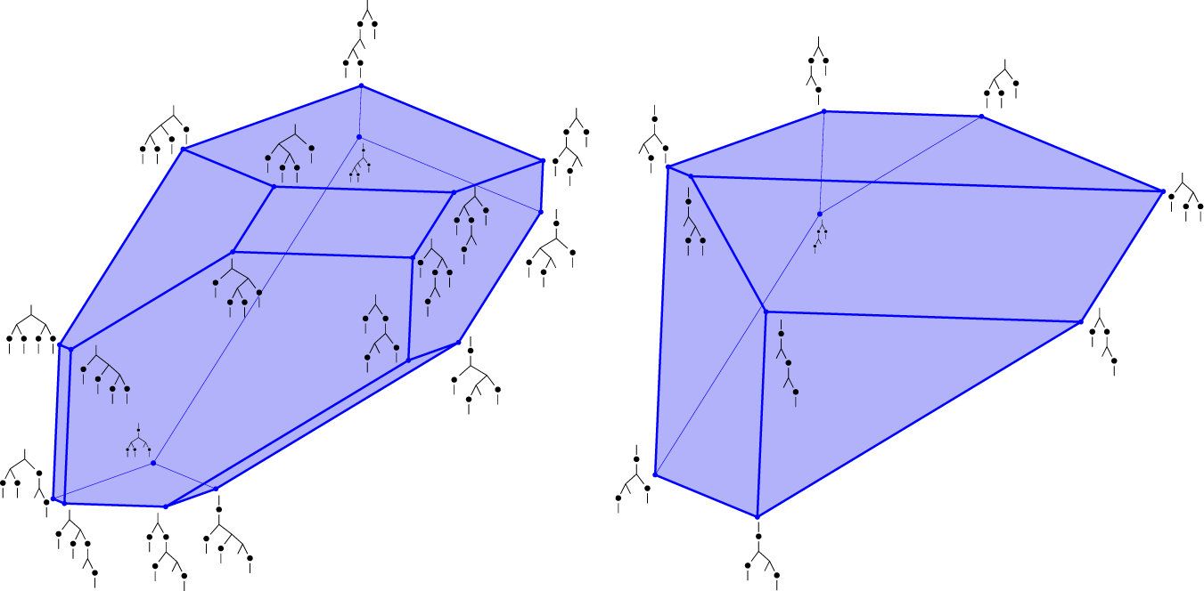
 (see Figure 14). For this, we first construct the
 , associating to each pebble tree a polyhedral cone in a natural but subtle way, and then prove that this fan is the normal fan of a polytope by checking that its wall-crossing inequalities are satisfiable.
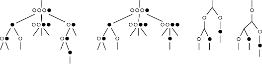
Some
$\circ $
 -balanced and
$\bullet $
 -unbalanced
$\{\circ , \bullet \}$
 -pebble trees. The first two are related by a contraction (Section 2.2), while the last two are related by a flip (Section 2.4).

Figure 1: Long description
The diagram displays four pebble trees arranged horizontally. Each tree consists of nodes represented by horizontal clusters of open circles and solid black dots, connected by lines.
1. The first tree on the far left is circle-balanced. The root node has three open circles and one black dot. It branches into three child nodes. The left child has one black dot and branches further. The middle child has two open circles and two black dots. The right child has one open circle and one black dot.
2. The second tree is related to the first by a contraction. It maintains a similar root structure but shows a more condensed branching pattern in the middle and right sections, with the rightmost leaf node containing two open circles and two black dots.
3. The third tree is dot-unbalanced and has a simpler, more vertical structure. The root is a single line branching into two nodes, each represented by a single open circle. These further branch into nodes containing a mix of single open circles or single black dots.
4. The fourth tree on the far right is related to the third by a flip transformation. The branching structure is mirrored or rotated compared to the third tree, with the primary vertical stem shifting position and the distribution of single open circles and black dots rearranged across the levels.
Our construction recovers the combinatorics and geometry of the permutahedra and associahedra in two degenerate situations. On the one hand, pebble trees with a single leaf can be seen as ordered partitions of their balanced colors, and the pebble tree polytope is the permutahedron. On the other hand, pebble trees with no pebbles are Schröder trees, and the pebble tree polytope is the associahedron. But the special situation which motivated this article is when there is exactly one color of pebbles. The pebble trees are then in bijection with some specific oriented planar trees considered by K. Poirier and T. Tradler in [Reference Poirier and TradlerPT18] for the combinatorics of algebraic structures endowed with a binary product and a co-inner product. These structures are closely connected to the
$V_\infty $
 -algebras of T. Tradler and M. Zeinalian [Reference Tradler and ZeinalianTZ07] that arose in a tentative algebraic model for string topology operations defined by M. Chas and D. Sullivan [Reference Chas and SullivanCS99]. It is proved in [Reference Poirier and TradlerPT18] that the contraction posets on these oriented planar trees are face lattices of the
 , which are polytopal complexes refining the boundary complex of the Cartesian product of an associahedron with a simplex. We prove here that all assocoipahedra can actually be realized as convex polytopes using faces of pebble tree polytopes (see Figure 15).
The paper is organized as follows. Section 2 is devoted to the combinatorics of pebble trees. In Section 2.1, we provide more precise definitions and notations for pebble trees, we introduce some natural maps between families of pebble trees, and we give the precise bijection with the oriented planar trees of [Reference Poirier and TradlerPT18]. We introduce in Section 2.2 the pebble tree contraction poset, prove in Section 2.3 that it is the face poset of a pseudomanifold called the pebble tree complex, and discuss in Section 2.4 the adjacency graph of this complex called the pebble tree flip graph. Section 3 is devoted to the geometry of pebble trees. After quickly reminding the reader some geometric preliminaries in Section 3.1, we construct the pebble tree fan in Section 3.2 and the pebble tree polytope in Section 3.3. Finally, Section 4 is devoted to the numerology of pebble trees. We compute the generating functions of the maximal pebble trees in Section 4.1 and of all the pebble trees in Section 4.2, and gather explicit expansions of these generating functions in Section 4.3. While the methods are standard computations based on generatingfunctionology [Reference Flajolet and SedgewickFS09], the results reveal a few surprises.
2 Pebble tree combinatorics
In this section, we define pebble trees (Section 2.1) and study the pebble tree contraction poset (Section 2.2), the pebble tree complex (Section 2.3), and the pebble tree flip graph (Section 2.4).
2.1 Pebble trees
Recall that an  is either a
 or a
 with an ordered list of subtrees. These subtrees are the
 of the node, and this node is the
 of these subtrees. As we only consider ordered trees, we omit the adjective ordered and only say tree. For a node n in a tree T, we denote by
$T_n$
 the subtree of T rooted at n. For a subtree S, we denote by
 the set of leaves of S.
Definition 2.1 For a finite set of colors  , a
 is a tree with pebbles colored by
 placed on its nodes such that
-
(1) each leaf receives no pebble, each node with a single child receives at least one pebble, and each node with at least two children receives arbitrary many pebbles (possibly none),
-
(2) for each subtree S and each color
 , the number of leaves minus the number of pebbles of color in S is either
$0$
or
$1$
.
 , the number of leaves minus the number of pebbles of color
 in S is either


Example 2.1 Two classical combinatorial objects are extreme examples of pebble trees:
-
• pebble trees with a single leaf can be seen as ordered partitions of their pebble colors,
-
• pebble trees with no pebbles (meaning
) are Schröder trees (where each node has either none or at least two children).
 ) are Schröder trees (where each node has either none or at least two children).
Some more generic examples of pebble trees are illustrated in Figure 1. Note that all our pictures of trees start with a vertical half-edge attached to the root, and end with half-edges representing the leaves.
Notation 2.2 We call  the pebbles of color
 . We call
 of a subtree S the difference
 between the number of leaves and the number of
 -pebbles of S. We say that S is
 (resp.
 ) if
 (resp.
 ). We denote by
 (resp.
 ) the set of colors
 for which S is
 -balanced (resp.
 -unbalanced).
Notation 2.3 We denote by  the set of all pebble trees with leaves L and pebble colors
 , and by
 the subset of B-balanced and U-unbalanced pebble trees of
 for any
 . For
$\ell , b, u \in \mathbb {N}$
 , we define
 as
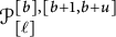 . In this case, we label the leaves by
$[\ell ]$
 from left to right, the balanced pebble colors by
$[b]$
 and the unbalanced pebble colors by
$[b+1,b+u]$
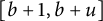 . Note that
 is isomorphic to
 for arbitrary
$L, B, U$
 with
$|L| = \ell $
 ,
$|B| = b$
 and
$|U| = u$
 . It is however convenient to keep the notation
 to define certain operations on pebble trees (see Definitions 2.2–2.5) and for recursive decompositions of the pebble trees (see Section 4).
Remark 2.4 Some immediate consequences of Definition 2.1:
-
•
is finite for any L and , thus is finite for any
${\ell , b, u \in \mathbb {N}}$
. -
• The number of
-pebbles at a node p with children
$c_1, \dots , c_k$
is . Hence, the number of -unbalanced children of p is the number of -pebbles at p, plus
$1$
if p is -unbalanced. -
• Each unary node has at least one pebble, and at most one of each color.
-
• There is no consecutive chain formed by
unary nodes
 is finite for any L and
 , thus
 is finite for any

 -pebbles at a node p with children

 . Hence, the number of
 -unbalanced children of p is the number of
 -pebbles at p, plus

 -unbalanced.
 unary nodes
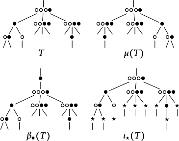
We now define five natural maps between pebble trees (see Figures 2 and 3), that will induce isomorphisms in Propositions 2.10, 2.17, and 3.11. In Definitions 2.4 and 2.6, we call  -leaf the only pebble tree of
 , i.e., whose root has a single pebble of color
 and a single child which is a leaf.
A
$\circ $
 -balanced and
$\bullet $
 -unbalanced
$\{\circ , \bullet \}$
 -pebble tree (left), the
$\circ $
 -balanced and
$\bullet $
 -unbalanced
$\{\circ , \bullet \}$
 -pebble tree obtained by mirroring it (middle left), the
$\{\circ ,\bullet \}$
 -balanced
$\{\circ , \bullet \}$
 -pebble tree obtained by
$\bullet $
 -balancing it (middle right), and the
$\{\circ ,\star \}$
 -balanced and
$\bullet $
 -unbalanced
$\{\circ , \bullet , \star \}$
 -pebble tree obtained by
$\star $
 -inserting it (right).

Figure 2: Long description
The figure contains four panels labeled T, mu(T), beta sub bullet (T), and iota sub star (T).
* Top-left panel T: A tree with a root node containing three open circles and one solid bullet. It branches into three children. The left child is a solid bullet, the middle child has two open circles and two solid bullets, and the right child has one open circle and three solid bullets. Further branching occurs at the leaf level with various combinations of open and solid circles.
* Top-right panel mu(T): A mirrored version of tree T. The root node remains the same, but the horizontal order of the three main branches is reversed. The rightmost branch of T is now on the left, and the leftmost branch of T is now on the right.
* Bottom-left panel beta sub bullet (T): A modified version of tree T where a new root node consisting of a single solid bullet is added above the original root. The original root node and its entire structure are now the sole child of this new bullet node.
* Bottom-right panel iota sub star (T): A modified version of tree T where star symbols have been inserted. The root and first level of branching remain similar to T. However, at the leaf level, several nodes are replaced or augmented with star symbols. Specifically, the middle and right branches now terminate in nodes containing three star symbols each, and additional stars are placed at the very bottom of the leaf stems.
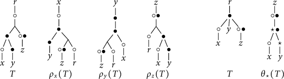
A fully balanced
$\{\circ , \bullet \}$
 -pebble tree and the fully balanced
$\{\circ , \bullet \}$
 -pebble trees obtained by rerooting it at leaves x, y and z respectively (left). A fully unbalanced
$\{\circ , \bullet \}$
 -pebble tree and the fully balanced
$\{\circ ,\bullet ,\star \}$
 -pebble tree obtained by
$\star $
 -uprooting it (right).

Figure 3: Long description
The diagram is divided into two main sections.
The left section contains four trees labeled T, rho sub x (T), rho sub y (T), and rho sub z (T).
- Tree T is rooted at r with an open circle node. It branches into a left subtree with a solid dot and a right subtree with an open circle and solid dot pair. Leaves are x, y, and z.
- Tree rho sub x (T) is rerooted at x. The path from x to the new root shows a sequence of open and solid nodes, with leaves y, z, and r at the bottom.
- Tree rho sub y (T) is rerooted at y, showing a vertical spine of two solid dots before branching to leaves z, r, and x.
- Tree rho sub z (T) is rerooted at z, starting with an open circle and solid dot pair at the root, branching down to leaves r, x, and y.
The right section contains two trees labeled T and theta sub star (T).
- The second Tree T is rooted at r with a solid dot, branching directly to leaves x, y, and z. Leaf x has an open circle, and leaf z has an open circle and solid dot pair.
- Tree theta sub star (T) is the result of star-uprooting. It is rooted at z with an open circle and solid dot pair. The structure below includes nodes marked with star symbols and open circles, leading to leaves x and y at the base.
Definition 2.2 The  sends a pebble tree T of
 to the pebble tree
$\mu (T)$
 of
 obtained by a vertical symmetry of the tree, meaning that
$\mu (T)$
 is defined inductively by
-
• if T is just a leaf, then $\mu (T)$
is just a leaf, -
• if T is a node with pebbles P and children $C_1, \dots , C_j$
, then
$\mu (T)$
is a node with pebbles P and children
$\mu (C_j), \dots , \mu (C_1)$
.



Definition 2.3 If  , the
 sends a pebble tree T of
 to the pebble tree
 of
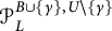 whose root has a single pebble of color
 and a single child T.
Definition 2.4 If  , the
 sends a pebble tree T of
 to the pebble tree
 of
 obtained from T by replacing each leaf by a
 -leaf.
Definition 2.5 If
$x \in L$
 and
$U = \varnothing $
 , the
 sends a pebble tree T of
 to the pebble tree
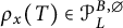 obtained by hanging T from its leaf x. In other words,
$\rho _x(T)$
 is the tree on the nodes of T where the children of each node p of T are the neighbors c of p in T so that x is in the connected component of p in the tree T were we have deleted the edge joining p to c.
Definition 2.6 If
$\ell> 1$
 ,
$B = \varnothing $
 and
 , the
 sends a pebble tree T of
 to the pebble tree
 of
 obtained from T by first hanging T from its rightmost leaf, then deleting the leftmost leaf and placing a
 -pebble at its parent, and finally replacing all remaining leaves except the first by a
 -leaf.
Finally, our next three remarks connect pebble trees with other relevant families of trees.
Remark 2.5 Consider a word  starting with
 (here,
 and
 stand for incoming and outgoing). An
 is a rooted oriented planar tree such that
-
• labeling the external arrows counterclockwise starting from the root, the ith arrow is incoming if
and outgoing if , -
• each internal node has at least one outgoing arrow,
-
• there is no node with precisely one incoming and one outgoing arrow.
 and outgoing if
 ,
These trees arise in the combinatorics of algebras endowed with a binary product and a co-inner product. They are studied in details in [Reference Poirier and TradlerPT18]. It turns out that they can be understood from pebble trees.
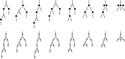
First, as illustrated in Figure 4, there are simple bijections between the pebble trees of  and the
 -trees (meaning the trees where all leaves are outgoing):
-
• Starting from a pebble tree
, orient each arc
$(p,c)$
joining a parent p to one of its children c in T from c to p if c is balanced, and from p to c if c is unbalanced, orient the root and leaves outward, and forget all pebbles. -
• Starting from a
-tree, place at each node one less pebbles than its outdegree, and forget the orientations.
 , orient each arc

 -tree, place at each node one less pebbles than its outdegree, and forget the orientations.
In the present paper, we prefer our interpretation as pebble trees as it enables us to consider several pebble colors simultaneously.
Examples of the bijection between the pebble trees of  and the
 -trees.

Figure 4: Long description
The diagram consists of 16 mathematical tree structures arranged in two horizontal rows of eight.
Top Row: Eight pebble trees of Script capital P super 1, 0 sub 3. These are rooted trees where nodes are represented by black dots (pebbles) or branching junctions.
* The first tree on the left has a complex branching structure with four pebbles distributed along different levels.
* Moving right, the trees vary in depth and pebble placement, with some having pebbles at the root and others at leaf nodes.
* The eighth tree on the far right is the simplest, consisting of a single root node with three pebbles placed horizontally across three branching paths.
Bottom Row: Eight directed o super 4-trees. Each tree in this row corresponds directly to the pebble tree above it.
* These trees use arrows on their edges to indicate directionality.
* Upward-pointing arrows represent internal structure, while downward-pointing arrows indicate terminal paths.
* The branching patterns in this row mirror the connectivity of the pebble trees above, demonstrating the one-to-one correspondence (bijection) between the two sets of mathematical objects.
Consider now an arbitrary signature
$\alpha $
 . Although not explicit in [Reference Poirier and TradlerPT18], there is a clear map from
$\alpha $
 -trees to
 -trees, which consists in replacing each incoming external arrow (like
 ) by a node with a pair of outgoing arrows (like
 ). This leads to a bijection between the
$\alpha $
 -trees and the pebble trees of
 where the parent of the ith leaf is a unary node marked with a pebble.
Remark 2.6 The reader familiar with the bijective combinatorics of planar maps might also see some connections with the
$\beta $
 -trees of [Reference Jacquard and SchaefferJS98, Reference Cori and SchaefferCS03]. Indeed, labeling each node p of a pebble tree by the pebble default
 , we obtain a
$\beta (1,1)$
 -tree. However, this map is clearly injective but not surjective, and the additional condition given by the pebble trees is unclear on
$\beta (1,1)$
 -trees.
Remark 2.7 There is also a natural map from the pebble trees of  to the painted trees corresponding to the faces of the multiplihedron [Reference StasheffSta70, Reference ForceyFor08, Reference Chapoton and PilaudCP22]. Namely, we can just forget all pebbles which have a pebble on the path to the root of the pebble tree to obtain a painted tree.
2.2 Pebble tree contraction poset
We now define the contraction poset on pebble trees, and will see that it is the face poset of a simplicial complex in Section 2.3 and of a polytope in Section 3.3.
Definition 2.7 For any node c (not a leaf, nor the root) with parent p in a pebble tree T, the  of c in T is the pebble tree
$T/c$
 obtained by replacing c by its children in the list of children of p and adding to p the pebbles of c. The

 is the poset of contractions on pebble trees of
 .
Example 2.8 In the extreme situations of Example 2.1:
-
• the pebble tree contraction poset
is the refinement poset on ordered partitions of
$[b]$
, -
• the pebble tree contraction poset
is the contraction poset on Schröder trees with
$\ell $
leaves.
 is the refinement poset on ordered partitions of

 is the contraction poset on Schröder trees with

The pebble tree contraction posets  and
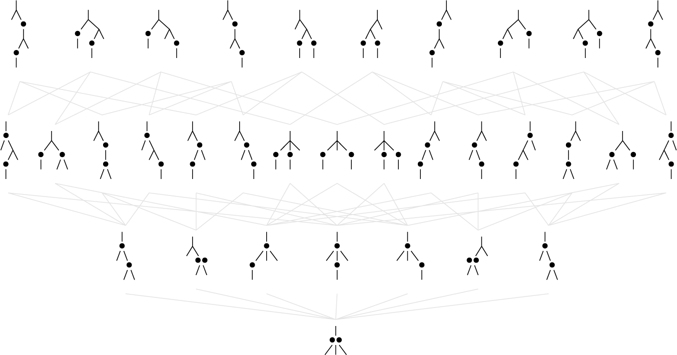
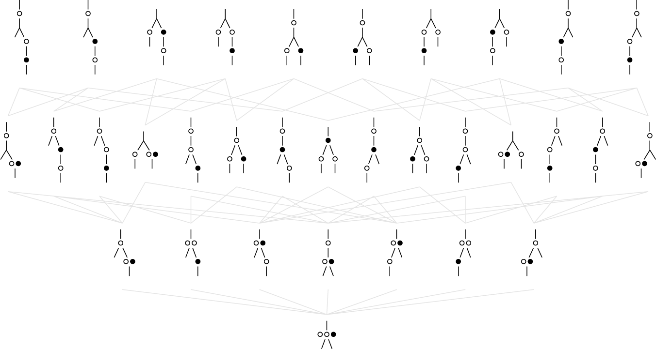
 are illustrated in Figures 5 and 6. The fact that
 and
 are isomorphic can be seen applying successively Points (5), (4), and (2) of Proposition 2.10 below.
The pebble tree contraction poset  .

Figure 5: Long description
The diagram consists of four horizontal levels of tree structures connected by light gray lines indicating contraction relationships.
* At the bottom (Level 1) is a single base tree with two black dots (pebbles) placed at the root node where two branches meet.
* Level 2 contains seven distinct tree variations. These trees show the pebbles moving upward or onto different branches. Some trees have pebbles on edges, while others have them on nodes. They are connected to the base tree by gray lines radiating upward.
* Level 3 contains fifteen tree variations, showing further distribution and separation of the two pebbles across more complex branching structures. A dense web of gray lines connects Level 2 trees to these Level 3 configurations.
* The top (Level 4) contains ten tree variations. These represent the most expanded or terminal states in the poset, where pebbles are often located at the leaf nodes or high up on the branches. A final layer of intersecting gray lines connects Level 3 to Level 4.
The pebble tree contraction poset  .

Figure 6: Long description
A poset diagram organized into four horizontal levels connected by light gray diagonal lines indicating contraction relationships.
* Level 1 (Bottom): A single root node consisting of a vertical line segment leading to a cluster of three circles (two white, one black) above a small inverted V shape.
* Level 2: Seven distinct tree structures. Each structure features a vertical stem branching into smaller nodes. The nodes contain combinations of white and black circles (pebbles) positioned at different vertices and along the edges.
* Level 3: Fifteen tree structures. These represent intermediate contraction states. The trees show increased branching complexity compared to the level below, with pebbles distributed across primary and secondary branches.
* Level 4 (Top): Ten tree structures. These are the most expanded forms in the poset. Each tree has a clear hierarchical branching structure with a single pebble (either black or white) placed at specific leaf or internal nodes, while other nodes remain empty (white circles).
The connections between levels form a complex web, showing how multiple expanded trees can contract into the same lower-level configurations.
Remark 2.9 Observe that:
-
• The set of pebble trees
is clearly closed under contraction. Hence, the pebble tree contraction poset is a simplicial poset (a poset where each interval is a boolean algebra). -
• The pebble tree contraction poset is ranked: the rank of a pebble tree is its number of nodes.
-
• The
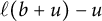
pebble trees of are the pebble trees with only unary nodes containing a single pebble and binary nodes containing no pebble (hence, they have
$\ell (b+u)-u$
unary nodes and
$\ell -1$
binary nodes, thus rank
$\ell (1 + b + u) - u - 1$
). -
• The
pebble tree of is the corolla with
$\ell $
leaves and
$\ell (b+u)-u$
pebbles at the root (hence it has rank
$1$
).
 is clearly closed under contraction. Hence, the pebble tree contraction poset is a simplicial poset (a poset where each interval is a boolean algebra).
 pebble trees of
 are the pebble trees with only unary nodes containing a single pebble and binary nodes containing no pebble (hence, they have
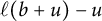


 pebble tree of
 is the corolla with


Observe now that the mirroring, balancing, inserting, rerooting and uprooting maps of Definitions 2.2–2.6 obviously commute with contractions. This implies the following statement.
Proposition 2.10 Consider the operations of Definitions 2.2–2.6.
-
(1) The mirroring map of Definition 2.2 defines a poset automorphism of
. -
(2) If $u> 1$
, the balancing map of Definition 2.3 defines a poset isomorphism from the pebble tree contraction poset to a principal upper set of the pebble tree contraction poset . Hence, is isomorphic to a principal upper set of . -
(3) The inserting map of Definition 2.4 defines a poset isomorphism from the pebble tree contraction poset
to a principal upper set of the pebble tree contraction poset . -
(4) The rerooting maps of Definition 2.5 define poset automorphisms of
. -
(5) If $\ell> 1$
, the uprooting map of Definition 2.6 defines a poset isomorphism from the pebble tree contraction poset to a principal upper set of the pebble tree contraction poset .
 .

 to a principal upper set of the pebble tree contraction poset
 . Hence,
 is isomorphic to a principal upper set of
 .
 to a principal upper set of the pebble tree contraction poset
 .
 .

 to a principal upper set of the pebble tree contraction poset
 .
Finally, we connect the
$\alpha $
 -trees of [Reference Poirier and TradlerPT18] to an upper set of the pebble tree contraction poset.
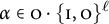
Remark 2.11 Following Remark 2.5, observe that for any signature 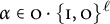 , the
$\alpha $
 -tree contraction poset is isomorphic to the principal upper set of the pebble tree contraction poset
 generated by the pebble tree whose root has
 pebbles and
$\ell $
 children, and whose ith children is a leaf if
 and a unary node with one pebble and a leaf if
 .
Remark 2.12 The following observations are consequences of Remarks 2.5 and 2.11 and Proposition 2.10:
-
• the
-tree contraction poset is isomorphic to the pebble tree contraction poset , -
• for any
with a single occurrence of , the
$\alpha $
-tree contraction poset is isomorphic to the pebble tree contraction poset , -
• for
or , the
$\alpha $
-tree contraction poset is isomorphic to the pebble tree contraction poset (i.e., the contraction poset on Schröder trees).
 -tree contraction poset is isomorphic to the pebble tree contraction poset
 ,
 with a single occurrence of
 , the

 ,
 or
 , the

 (i.e., the contraction poset on Schröder trees).
2.3 Pebble tree complex
As mentioned in Remark 2.9, the pebble tree contraction poset  is a simplicial poset. We now construct the corresponding simplicial complex. For a pebble tree in
 , recall that we label the leaves by
$[\ell ]$
 from left to right, the balanced pebble colors by
$[b]$
 , and the unbalanced pebble colors by
$[b+1,b+u]$
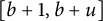 . Recall also that we denote by
 and
 the sets of leaves and of balanced colors in a subtree S. We will moreover need the following notation and definition, which might be mysterious at first sight, but aims at generalizing Example 2.14 and will be crucial in Section 3.2.
Notation 2.13 For an interval  and a subset
$B \subseteq [b+u]$
 , we define the sets

Definition 2.8 The 
 is the simplicial complex whose simplices are the sets
 for all pebble trees
 , where
 .
Example 2.14 In the extreme situations of Example 2.1:
-
• the simplices of the pebble tree complex
are the flags
$B_1 \subsetneq B_2 \subsetneq \dots \subsetneq B_k \subseteq [b]$
, -
• the simplices of the pebble tree complex
are the collections of pairwise nested or non-adjacents intervals of
$[\ell -1]$
.
 are the flags

 are the collections of pairwise nested or non-adjacents intervals of

Figure 7 illustrates some more generic examples of simplices
$\Lambda (T)$
 . Note that in these trees, the white color
$\circ $
 is labeled
$1$
 while the black color
$\bullet $
 is labeled
$2$
 .
Some
$\circ $
 -balanced and
$\bullet $
 -unbalanced
$\{\circ , \bullet \}$
 -pebble trees T and the associated simplices
$\Lambda (T)$
 . Each node n of T is labeled by the concatenation of the elements of the set
$\lambda (T_n)$
 .

Figure 7: Long description
The figure displays five distinct tree diagrams arranged horizontally. Each tree starts with a root at the top and branches downward. Nodes are marked with either open circles or solid black circles (pebbles) and are accompanied by numeric strings representing the set lambda of T sub n.
* The first tree on the left has a root labeled 1 2 3 4 5. It branches into a left node labeled 1 3 4 with an open circle and a right node labeled 5 8 with an open circle. The left node further branches into a node labeled 1, which then splits into a node labeled 3 with an open circle and a node labeled 7 with a solid circle. The right node branches to a node labeled 8 with a solid circle.
* The second tree has a root labeled 1 2 3 4 5 with an open circle. It descends to a node labeled 1 2 with an open circle, which branches into a node labeled 1 and a node labeled 8 with a solid circle. The node labeled 1 further branches into a node labeled 3 with an open circle and a node labeled 7 with a solid circle.
* The third tree has a root labeled 1 2 3 4 5 followed by two open circles. It branches into a node labeled 1 and a node labeled 8 with a solid circle. The node labeled 1 branches into a node labeled 3 with an open circle and a node labeled 7 with a solid circle.
* The fourth tree has a root labeled 1 2 3 4 5. It branches into a left node labeled 1 3 4 6 7 with a solid circle and a right node labeled 5 with an open circle. The left node branches into a node labeled 3 with an open circle and a node labeled 7 with a solid circle. The node labeled 7 further descends to a node labeled 4 with an open circle.
* The fifth tree on the far right is a single-level structure. The root is labeled 1 2 3 4 5 followed by three open circles and two solid circles. Three short vertical lines descend from this root node without further labels.
Proposition 2.15 The pebble tree complex  is a pseudomanifold, whose face poset is isomorphic to the pebble tree poset
 .
Proof Observe first that
$\Lambda (T/n) = \Lambda (T) \smallsetminus \{\lambda (T_n)\}$
 for any node n (not a leaf, nor the root) in a pebble tree T. Hence, the face poset of
 is indeed isomorphic to
 . We thus obtain that
 is a pure simplicial complex since
 is a ranked simplicial poset. It remains to prove that
 is a pseudomanifold, meaning that any ridge (i.e., codimension
$1$
 face) is contained in precisely two facets (i.e., maximal dimensional faces). Consider thus a pebble tree of corank
$1$
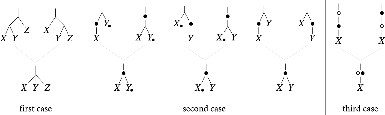
 , and let p be the only node which is neither unary with a pebble, nor binary with no pebble. We want to prove that there are two ways to open p, meaning to replace p by an edge whose contraction gives back p. We distinguish three cases:
-
• If p has three children and no pebble, then there are two ways to open p as usual (see Figure 8 (left)) and it does not matter whether p and its children are balanced or not for each pebble color.
Figure 8:The pebble tree complex is a pseudomanifold. All possible corank $1$
pebble trees are obtained by contracting precisely two maximal pebble trees. In the second (resp. third) picture, we mark Y (resp. X) with a
$\bullet $
to indicate that it is
$\bullet $
-balanced. Neither X nor Y are
$\bullet $
-balanced in the fourth picture.Figure 8: Long description
The diagram consists of five panels separated by vertical lines. Each panel shows two bifurcating trees at the top that converge via light gray lines into a single contracted tree at the bottom.
* Panel 1 labeled first case. Top left tree has leaves X, Y, and Z where X and Y share a node. Top right tree has leaves X, Y, and Z where Y and Z share a node. The bottom tree is a single node with three leaves X, Y, and Z.
* Panel 2. Top left tree has leaves X and Y with a dot on the left branch and a dot next to Y. Top right tree has leaves X and Y with a dot on the main stem and a dot next to Y. The bottom tree has leaves X and Y with a dot at the root and a dot next to Y.
* Panel 3 labeled second case. Top left tree has leaves X and Y with a dot next to X and a dot on the right branch. Top right tree has leaves X and Y with a dot on the main stem and a dot next to X. The bottom tree has leaves X and Y with a dot at the root and a dot next to X.
* Panel 4. Top left tree has leaves X and Y with a dot on the left branch. Top right tree has leaves X and Y with a dot on the left branch. The bottom tree has leaves X and Y with a dot at the root.
* Panel 5 labeled third case. Top left tree has a single leaf X with an open circle above a solid dot on the stem. Top right tree has a single leaf X with a solid dot above an open circle on the stem. The bottom tree has a single leaf X with an open circle and a solid dot side-by-side at the root.
-
• If p has two children and a
-pebble, then p is -balanced, and there are still two ways to open p depending on whether its children are -balanced or not (see Figure 8 (middle)). -
• If p has one child and two pebbles of different colors, then there are still two ways to open p choosing which pebble goes in the parent and which pebble goes in the child (see Figure 8 (right)).


 -pebble, then p is
 -balanced, and there are still two ways to open p depending on whether its children are
 -balanced or not (see Figure
Remark 2.16 In contrast to the special situations of Example 2.1, the pebble tree complex is not flag in general. For instance,  and
 are not flag.
Finally, we translate Proposition 2.10 and Remark 2.11 to the pebble tree complex.
Proposition 2.17 Consider the operations of Definitions 2.2–2.6.
-
(1) The map defined by $\ell j + i - \delta _{j \ne 0} \mapsto \ell (j + 1) - i$
for any
${(i,j) \in ([\ell ] \times [0,b+u]) \smallsetminus \{(\ell ,0)\}}$
induces an automorphism of the pebble tree complex . -
(2) If $u> 1$
, the pebble tree complex is isomorphic to the link of the face
${[\ell ] \boxtimes [b]}$
in the pebble tree complex . Hence, is isomorphic to a link of . -
(3) The pebble tree complex
is isomorphic to the link of the face
$\left \{ \{i\} \boxtimes [1] \;\middle |\; i \in [\ell ] \right \}$
in the pebble tree complex . -
(4) The rerooting maps of Definition 2.5 induce automorphisms of the pebble tree complex
. -
(5) If $\ell> 1$
, the pebble tree complex is isomorphic to the link of the face
$\left \{ \{i\} \boxtimes [1] \;\middle |\; i \in [2,\ell -1] \right \}$
in the pebble tree complex .


 .

 is isomorphic to the link of the face

 . Hence,
 is isomorphic to a link of
 .
 is isomorphic to the link of the face

 .
 .

 is isomorphic to the link of the face

 .
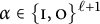 , the

 in the pebble tree complex
 .
2.4 Pebble tree flip graph
As the pebble tree complex  is a pseudomanifold by Proposition 2.15, it is natural to consider its dual graph.
Definition 2.9 Two maximal pebble trees T and
$T'$
 of
 are related by a
 if there are nodes n of T and
$n'$
 of
$T'$
 such that the following equivalent conditions hold:
-
• the contraction $T/n$
coincides with the contraction
$T'/n'$
, -
• $\Lambda (T) \smallsetminus \{\lambda (T_n)\} = \Lambda (T') \smallsetminus \{\lambda (T^{\prime }_{n'})\}$
.



All possible types of flips are illustrated in Figure 9. The  is the graph whose vertices are the maximal pebble trees of
 and whose edges are the flips between them.
All possible flips in a maximal pebble tree. In the second (resp. third) picture, we mark Y (resp. X) with a
$\bullet $
 to indicate that it is
$\bullet $
 -balanced. Neither X nor Y are
$\bullet $
 -balanced in the fourth picture.

Example 2.19 In the extreme situations of Example 2.1:
-
• the flip graph on
is the graph of adjacent transpositions on permutations of
$[b]$
, -
• the flip graph on
is the rotation graph on binary trees with
$\ell $
leaves.
 is the graph of adjacent transpositions on permutations of

 is the rotation graph on binary trees with

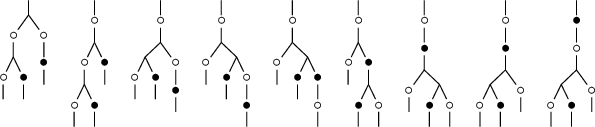
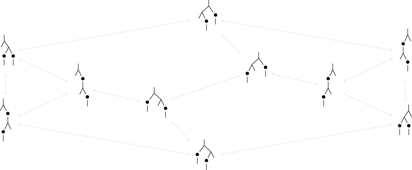
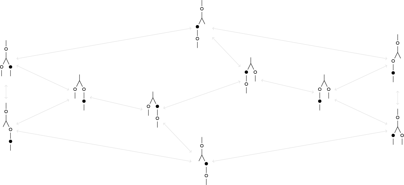
These extreme situations correspond to the right and left cases of Figure 9 respectively. Figure 10 illustrates a sequence of flips in maximal pebble trees of  . Figures 11 and 12 illustrate the flip graphs on maximal pebble trees of
 and
 (which are isomorphic by Proposition 2.10 as already mentioned before).
A sequence of flips in maximal
$\circ $
 -balanced and
$\bullet $
 -unbalanced
$\{\circ , \bullet \}$
 -pebble trees.

Figure 10: Long description
The diagram displays nine rooted trees in a horizontal row. Each tree consists of nodes represented by open circles or solid black bullets, connected by vertical and diagonal lines.
* The first tree on the left has a bifurcating root leading to two open circle nodes. The left branch splits again into an open circle and a black bullet. The right branch ends in a black bullet.
* Moving right, the second through sixth trees show a gradual shift in the branching structure. The root node becomes a single open circle with a vertical stem before branching. Black bullets shift positions from lower leaf nodes to higher internal nodes.
* In the seventh and eighth trees, the structure becomes more elongated. A black bullet appears higher up the main vertical stem, and the branching occurs lower down the structure.
* The ninth tree on the far right shows the final state where a black bullet is positioned at the very top of the vertical stem, followed by an open circle, which then branches into a complex lower structure with both open circles and black bullets at the terminal ends.
The flip graph on pebble trees of  .

The flip graph on pebble trees of  .

Figure 12: Long description
The graph consists of twelve nodes arranged in a large hexagonal ring with internal connections. Each node is a rooted tree with three leaves. Two pebbles, one black and one white, are placed on the edges or vertices of these trees.
* At the top center, a tree has a white pebble on the root edge and a black pebble on the right branch.
* Moving clockwise, the next node shows the black pebble shifted to the right leaf edge.
* The rightmost nodes show vertical stacks where pebbles move between the root and branch edges.
* At the bottom center, the white pebble is on the root edge and the black pebble is on the right leaf edge.
* The leftmost nodes mirror the right, with pebbles alternating between the root and the left branch edges.
* Internal arrows connect trees where a single ‘flip’ or pebble move transforms one configuration into another, such as moving a pebble from a branch to the root edge.
As the dual graph of a pure simplicial pseudomanifold, the pebble tree flip graph is regular. Its degree is
$\ell (1 + b + u) - u - 2$
 . As we will see in Theorem 3.8 that it is the graph of a simple polytope, it has the connectivity of its degree. Among various further properties of this graph that would require more investigations, we mention the following problem in connection to [Reference Sleator, Tarjan and ThurstonSTT88, Reference PourninPou14].
Problem 2.20 Evaluate the diameter of the flip graph on maximal pebble trees of  .
Finally, note that Proposition 2.10 and Remark 2.11 directly translate to morphisms between the flip graphs on the corresponding trees.
3 Pebble tree geometry
This section is devoted to the geometry of pebble trees. After quickly reminding the reader some geometric preliminaries (Section 3.1), we construct the pebble tree fan (Section 3.2) and the pebble tree polytope (Section 3.3).
3.1 Geometric preliminaries
We refer to [Reference ZieglerZie98] for a reference on polyhedral geometry, and only remind the basic notions needed later in the paper.
A (polyhedral)  is the positive span
 of a finite set
 of vectors of
$\mathbb {R}^d$
 or equivalently, the intersection of finitely many closed linear half-spaces of
$\mathbb {R}^d.$
 The
 of a cone are its intersections with its supporting hyperplanes. The
 (resp.
 ) are the faces of dimension
$1$
 (resp. codimension
$1$
 ). A cone is
 if its rays are linearly independent. A (polyhedral)
 $\mathcal{F} $
 is a set of cones such that any face of a cone of
$\mathcal{F} $
 belongs to
$\mathcal{F} $
 , and any two cones of
$\mathcal{F} $
 intersect along a face of both. A fan is
 if the intersection of its cones is the origin,
 if the union of its cones covers
$\mathbb {R}^d$
 , and
 if all its cones are simplicial.
Note that a simplicial fan defines a simplicial complex on its rays (the simplices of the simplicial complex are the subsets of rays which span a cone of the fan). Conversely, given a simplicial complex
$\Delta $
 with ground set V, one can try to realize it geometrically by associating a ray
 of
$\mathbb {R}^d$
 to each
$v \in V$
 , and the cone
 generated by the set
 to each
$\triangle \in \Delta $
 . To show that the resulting cones indeed form a fan, we will need the following statement, which can be seen as a reformulation of [Reference De Loera, Rambau and SantosDRS10, Corollary 4.5.20].
Proposition 3.1 Consider a closed simplicial pseudomanifold
$\Delta $
 with ground set V and a set of vectors
 of
$\mathbb {R}^d$
 , and define
 for any
$\triangle \in \Delta $
 . Then the collection of cones
 forms a complete simplicial fan of
$\mathbb {R}^d$
 if and only if
-
• there exists a vector ${\boldsymbol {v}}$
of
$\mathbb {R}^d$
contained in only one of the open cones for
$\triangle \in \Delta $
, -
• for any two adjacent facets $\triangle , \triangle '$
of
$\Delta $
with
$\triangle \smallsetminus \{v\} = \triangle ' \smallsetminus \{v'\}$
, we have
$\alpha _v \alpha _{v'}> 0$
where denotes the unique (up to rescaling) linear dependence on.


 for





 .
A  is the convex hull of finitely many points of
$\mathbb {R}^d$
 or equivalently, a bounded intersection of finitely many closed affine half-spaces of
$\mathbb {R}^d$
 . The
 of a polytope are its intersections with its supporting hyperplanes. The
 (resp.
 , resp.
 ) are the faces of dimension
$0$
 (resp. dimension
$1$
 , resp. codimension
$1$
 ).
The  of a face
 of a polytope
 is the cone generated by the normal vectors to the supporting hyperplanes of
 containing
 . Said differently, it is the cone of vectors
${\boldsymbol {c}}$
 of
$\mathbb {R}^d$
 such that the linear form
${\boldsymbol {x}} \mapsto \left \langle \, {\boldsymbol {c}} \; \middle | \; {\boldsymbol {x}} \, \right \rangle $
 on
 is maximized by all points of the face
 . The
 of
 is the set of normal cones of all its faces.
Consider now a complete simplicial fan
$\mathcal{F} $
 of
$\mathbb {R}^d$
 with rays
 and cones
 for
${\triangle \in \Delta }$
 , where
 as in Proposition 3.1. To realize the fan
$\mathcal{F} $
 , one can try to pick a height vector
 and consider the polytope ℙ
h
: = {
x
∈ℝ
d
| 〈
r
v |
x
〉≤h
v
for all v∈V}. The following classical statement characterizes the height vectors
${\boldsymbol {h}}$
 for which the fan
$\mathcal{F} $
 is the normal fan of this polytope
 . We borrow the formulation from [Reference Chapoton, Fomin and ZelevinskyCFZ02, Lemma 2.1].
Proposition 3.2 Let
$\mathcal{F} $
 be an essential complete simplicial fan in
$\mathbb {R}^n$
 with rays
 and cones
 for
$\triangle \in \Delta $
 . Then the following are equivalent for any height vector
${\boldsymbol {h}} \in \mathbb {R}^V$
 :
-
• The fan $\mathcal{F} $
is the normal fan of the polytope -
• For two adjacent facets $\triangle , \triangle '$
of
$\Delta $
with
$\triangle \smallsetminus \{v\} = \triangle ' \smallsetminus \{v'\}$
, the height vector
${\boldsymbol {h}}$
satisfies the $$\begin{align*}\alpha_v \, h_v + \alpha_{v'} \, h_{v'} + \sum_{w \in \triangle \cap \triangle'} \alpha_w \, h_w> 0 \end{align*}$$where
denotes the unique linear dependence on such that
$\alpha _v + \alpha _{v'} = 2$
.







 such that

3.2 Pebble tree fan
Fix
$\ell , b, u \in \mathbb {N}$
 and consider the intervals

whose union is the interval

We work in the Euclidean space
$\mathbb {R}^I$
 with canonical basis
$({\boldsymbol {e}}_i)_{i \in I}$
 . We denote by
 the characteristic vector of a subset
$J \subseteq I$
 . As our constructions actually live in the linear subspace

we define the vector

for each subset
$J \subseteq I$
 . It is immediate to check that these vectors satisfy the linear dependences

for any
$J, K \subseteq I$
 . Finally, we associate to any pebble subtree S the vector
 where
 and
 denote the sets of leaves and of balanced colors in S, and the operation
$\boxtimes $
 was defined in Definition 2.13. Note that
 when S is the entire tree T (because
 and
 so that
$\lambda (T) = I_0$
 ) or when S is a leaf i (because
 and
 so that
$\lambda (S) = \varnothing $
 ). We now use these vectors
 to construct the pebble tree fan.
Definition 3.1 The 
 is the collection of cones

for all pebble trees  , where
 .
Example 3.3 In the extreme situations of Example 2.1:
-
• the pebble tree fan
is the braid fan, with a ray for each proper subset
${\varnothing \neq J \subsetneq [b]}$
and a maximal cone for each permutation
$\sigma $
of
$[b]$
, defined by the inequalities
${x_{\sigma (1)} \le \dots \le x_{\sigma (b)}}$
, -
• the pebble tree fan
is the sylvester fan, with a ray for each proper interval J of
$[\ell ]$
and a maximal cone for each binary tree T, defined by the inequalities
$x_i \le x_j$
whenever there is a path from i to j in the tree T labeled in inorder and oriented toward its root.
 is the braid fan, with a ray
 for each proper subset

 for each permutation



 is the sylvester fan, with a ray
 for each proper interval J of

 for each binary tree T, defined by the inequalities

Note that the sylvester fan coarsens the braid fan: the cone  of the sylvester fan can also be obtained by glueing the cones
 of the braid fan corresponding to the linear extensions
$\sigma $
 of T.
Theorem 3.4 The pebble tree fan  is an essential complete simplicial fan in
$\mathbb {H}_\ell ^{b,u}$
 , whose face lattice is the pebble tree contraction poset
 .
The proof of Theorem 3.4 relies on the description of the linear dependences among adjacent maximal cones described in Lemma 3.6. To obtain these dependences, we need the following preliminary statement, where we use the operation
$\otimes $
 defined in Definition 2.13.
Lemma 3.5 For any maximal pebble tree S and any  , there are in S some distinct unary subtrees
$U_1, \dots , U_k$
 with children
$V_1, \dots , V_k$
 respectively such that
 .
Proof If a subtree U has a  -pebble and a unique child V, then we have
 because
 and
 . Hence, for any
 , if we denote by
$U_1, \dots , U_k$
 the closest descendants of S with a
 -pebble and by
$V_1, \dots , V_k$
 their respective children, then we have
 because
 . The result follows since
 .
Lemma 3.6 Let T and
$T'$
 be two adjacent maximal pebble trees and let S and
$S'$
 be the subtrees of T and
$T'$
 such that
$\Lambda (T) \smallsetminus \{\lambda (S)\} = \Lambda (T') \smallsetminus \{\lambda (S')\}$
 . Then there is a linear dependence among the rays
 associated with the subtrees R of T and
$T'$
 where the rays
 and
 both have coefficient
$1$
 .
Proof We analyse the five possible types of flips described in Figure 9. In all cases, we denote by R the parent of S and
$S'$
 . See Figure 13 here.
The four cases of the proof of 3.6.

Figure 13: Long description
The diagram presents five cases of tree transformations from left to right.
* Case 1: A tree with root R branching into S and Z, where S branches into X and Y, transforms into a tree with root R branching into X and S prime, where S prime branches into Y and Z.
* Case 2: A tree with root R branching into S and Y, with a black dot next to S and Y, and S leading to X, transforms into a vertical line with root R, a black dot, S prime, and a branch to X and Y with a black dot next to Y.
* Case 3: A tree with root R branching into X and S, with black dots next to X and S, and S leading to Y, transforms into a vertical line with root R, a black dot, S prime, and a branch to X and Y with a black dot next to X.
* Case 4: A tree with root R branching into S and Y, with a black dot next to S, and S leading to X, transforms into a tree with root R branching into X and S prime, with a black dot next to S prime, and S prime leading to Y.
* Case 5: A vertical line with root R, an open circle, S, and a black dot, leading to X, transforms into a vertical line with root R, a black dot, S prime, and an open circle, leading to X.


Since  (resp.
 , resp.
 ) is a linear combination of the rays
 for some subtrees P of S distinct from S (resp. of
$S'$
 distinct from
$S'$
 , resp. of Y) by Lemma 3.5, this is indeed a linear dependence among the rays
 associated with the subtrees Q of T and
$T'$
 where the rays
 and
 both have coefficient
$1$
 .

Again, we can develop  using Lemma 3.5, so that we indeed obtained a linear dependence among the rays
 for the subtrees Q of T and
$T'$
 where the rays
 and
 both have coefficient
$1$
 .
Case 3. The case of the third flip of Figure 13, is symmetric to Case 2.

We have

and moreover  . Using Lemma 3.5, we get

or, written differently

Now if R has no ancestor with a
$\bullet $
 -pebble, then using that
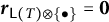 , we obtain similarly

where
-
• $U_1, \dots , U_k$
are the closest descendants of the root of T but not descendants of R which have a
$\bullet $
-pebble, -
• $V_1, \dots , V_k$
are the (unique) children of
$U_1, \dots , U_k$
respectively.


Proof of Theorem 3.4
Note that  is included in
$\mathbb {H}_\ell ^{b,u}$
 since all rays
 are. To prove that it is a complete simplicial fan, we just check the two criteria of Proposition 3.1. The second criterion is guaranteed by the description of the linear dependences in Lemma 3.6. For the first criterion, consider the vector

and a pebble tree T such that
${\boldsymbol {v}}$
 is contained in the interior of
 . As the last
$\ell -1$
 coordinates of
${\boldsymbol {v}}$
 are strictly larger than all other coordinates, each of the last
$\ell -1$
 leaves of T is preceded by a unary node with pebble colored by
$b+u$
 . Repeating the argument, we obtain that the first leaf of T is preceded by a chain of unary nodes with pebbles colored
$1, \dots , b$
 while each of the last
$\ell -1$
 leaves if T is preceded by a chain of unary nodes with pebbles colored
$1, \dots , b+u$
 . Finally, we obtain that the rest of the tree T is the left comb since it is the only Schröder tree whose cone in the sylvester fan contains the vector
 . Finally,
 is essential as the dimension of its cones matches the dimension of
$\mathbb {H}_\ell ^{b,u}$
 .
Remark 3.7 A few observations on the pebble tree fan:
-
• The simple descriptions of Example 3.3 for the braid fan and for the sylvester fan unfortunately fail for arbitrary $b,u \ge 0$
. Indeed, there is a natural way to label the nodes of a maximal pebble tree: label the binary nodes in inorder by
${[\ell -1]}$
and the unary nodes by the only leaf first covered by this pebble. This labeling yields a cone for each maximal pebble tree T, defined by
$x_i \le x_j$
whenever there is a directed path from i to j in the tree T oriented toward its root. However, the cones for all maximal pebble trees T do not define a complete simplicial fan (check out the case
$\ell = 2$
,
$b = 1$
and
$u = 0$
). In fact, our pebble tree fan is not refined by the braid fan in general -
• Our definition of the pebble tree fan
respects some symmetries of the pebble tree complex but not all. See Proposition 3.11 for a precise statement directly on polytopes. -
• Lemma 3.6 actually proves that the pebble tree fan
is smooth, meaning that the principal vectors spanning the rays of any maximal cone of form an integral basis of the space (in other words, the corresponding toric variety is smooth).


 for each maximal pebble tree T, defined by

 for all maximal pebble trees T do not define a complete simplicial fan (check out the case


 is not refined by the braid fan in general
 respects some symmetries of the pebble tree complex
 but not all. See Proposition
 is smooth, meaning that the principal vectors spanning the rays of any maximal cone of
 form an integral basis of the space (in other words, the corresponding toric variety is smooth).
3.3 Pebble tree polytope
Our next step is to construct a polytope whose normal fan is the pebble tree fan, using the criterion of Proposition 3.2.
Definition 3.2 A  on n is a map f from the subsets of
$[n]$
 to
$\mathbb {R}_{\ge 0}$
 such that
$f_\varnothing = 0$
 and

for any subsets A and B of
$[n]$
 . We then define

where the minimum ranges over all subsets A and B of
$[n]$
 such that
$A \not \subseteq B$
 and
$A \not \supseteq B$
 . Note that
-
• $\sum _{i \in [k]} f_{A_i} - f_A \ge (k-1) \cdot \Delta f$
for any
$A = \bigcup _{i \in [k]} A_i$
where
$A_1, \dots , A_k$
are pairwise disjoint, -
• $\Delta \lambda f = \lambda \Delta f$
for any scalar factor
$\lambda $
.

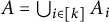


We say that f is  when
$\Delta f> 0$
 .
Theorem 3.8 Pick three strictly submodular functions f on
$\ell $
 , g on
$\ell $
 , and h on
$b+u$
 such that

Then the pebble tree fan  is the normal fan of the

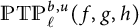 , the
$(\ell + \ell b + \ell u - u - 2)$
 -dimensional polytope defined in the subspace
$\mathbb {H}_\ell ^{b,u}$
 by the inequalities

for all
$1 \le s \le t \le \ell $
 and all
$B \subseteq [b+u]$
 .
Proof To shorten notations in this proof, we define for a maximal pebble subtree S

Observe that if V is the unique child of U, then
$\varphi _U - \varphi _V = g_U + h_U - h_V$
 because
 and
 . We just need to prove that the function
$\varphi $
 satisfies the wall-crossing inequalities of Proposition 3.2 for each of the linear dependences boxed in the proof of Lemma 3.6.
Case 1. By Lemmas 3.5 and 3.6, we have

for distinct unary subtrees
$U_1, \dots , U_k$
 of S (resp.
$U^{\prime }_1, \dots , U^{\prime }_{k'}$
 of
$S'$
 , resp.
$U^{\prime \prime }_1, \dots , U^{\prime \prime }_{k"}$
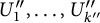 of Y) with respective children
$V_1, \dots , V_k$
 (resp.
$V^{\prime }_1, \dots , V^{\prime }_{k'}$
 , resp.
$V^{\prime \prime }_1, \dots , V^{\prime \prime }_{k"}$
 ). Since
 and
 , we have

where the last inequality holds since
$U_i \ne U_j$
 (resp.
$U^{\prime }_i \ne U^{\prime }_j$
 , resp.
$V^{\prime \prime }_i \ne V^{\prime \prime }_j$
 ) for
$i \ne j$
 , and the pebble tree T has
$\ell b + \ell u - u$
 unary subtrees. Since
$f, g, h$
 take non-negative values and
$\varphi _U - \varphi _V = g_U + h_U - h_V$
 when V is the unique child of U, we obtain that
$\varphi $
 satisfies the wall-crossing inequality

Case 2. By Lemma 3.6, we have

for distinct unary subtrees
$U_1, \dots , U_k$
 of Y with children
$V_1, \dots , V_k$
 , such that
 . Since
 , we obtain that

where the last inequality holds since
$S \ne U_i \ne U_j$
 for
$i \ne j$
 , and the subtree R has at most
$\ell b + \ell u - u$
 unary subtrees. Since
$f, g, h$
 take non-negative values and
${\varphi _U - \varphi _V = g_U + h_U - h_V}$
 when V is the unique child of U, we obtain that
$\varphi $
 satisfies the wall-crossing inequality

Case 3. Symmetric to Case 2.
Case 4. Assume first that R has an ancestor with a
$\bullet $
 -pebble. Then by Lemma 3.6, we have

Since  , we obtain that

where the last inequality holds since
$S \ne U_i \ne U_j \ne S'$
 for
$i \ne j$
 , and the subtree
$U_0$
 has at most
$\ell b + \ell u - u$
 unary subtrees. Since
$f, g, h$
 take non-negative values and
${\varphi _U - \varphi _V = g_U + h_U - h_V}$
 when V is the unique child of U, we obtain that
$\varphi $
 satisfies the wall-crossing inequality

Assume now that R has no ancestor with a
$\bullet $
 -pebble. Then we have

The wall-crossing inequality is thus even easier to satisfy since
$\varphi _{U_0} - \varphi _{V_0}$
 does not appear.
Case 5. By Lemma 3.6, we have

Since  and
 , we have

Remark 3.9 Note that the conditions of Theorem 3.8 are just sufficient conditions to ensure the wall-crossing inequalities. To find functions satisfying these conditions, pick three arbitrary strictly submodular functions
$f, g, h$
 and rescale first g by a factor
$4 (\ell b + \ell u - u + 1) \cdot \max h / \Delta g$
 , and then f by a factor
${(\ell b + \ell u - u) \cdot (\max g + \max h) / \Delta f}$
 . We just write
 if we want to consider
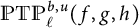 for arbitrary
$f,g,h$
 satisfying the conditions of Theorem 3.8.
Example 3.10 In the extreme situations of Example 2.1:
-
• the pebble tree fan
(a.k.a. braid fan) is the normal fan of the classical permutahedron, which can be obtained for
$h_B = \binom {b+1}{2} - \binom {|B|+1}{2}$
(the functions f and g are irrelevant here, since
$[s,t]$
is constant to
$[1]$
), -
• the pebble tree fan
(a.k.a. sylvester fan) is the normal fan of the classical associahedron [Reference Shnider and SternbergSS93, Reference LodayLod04], which can be obtained for
$f_X = \binom {\ell +1}{2} - \binom {|X|+1}{2}$
(the functions g and h are irrelevant here, since B is constant to
$\varnothing $
).
 (a.k.a. braid fan) is the normal fan of the classical permutahedron, which can be obtained for



 (a.k.a. sylvester fan) is the normal fan of the classical associahedron [


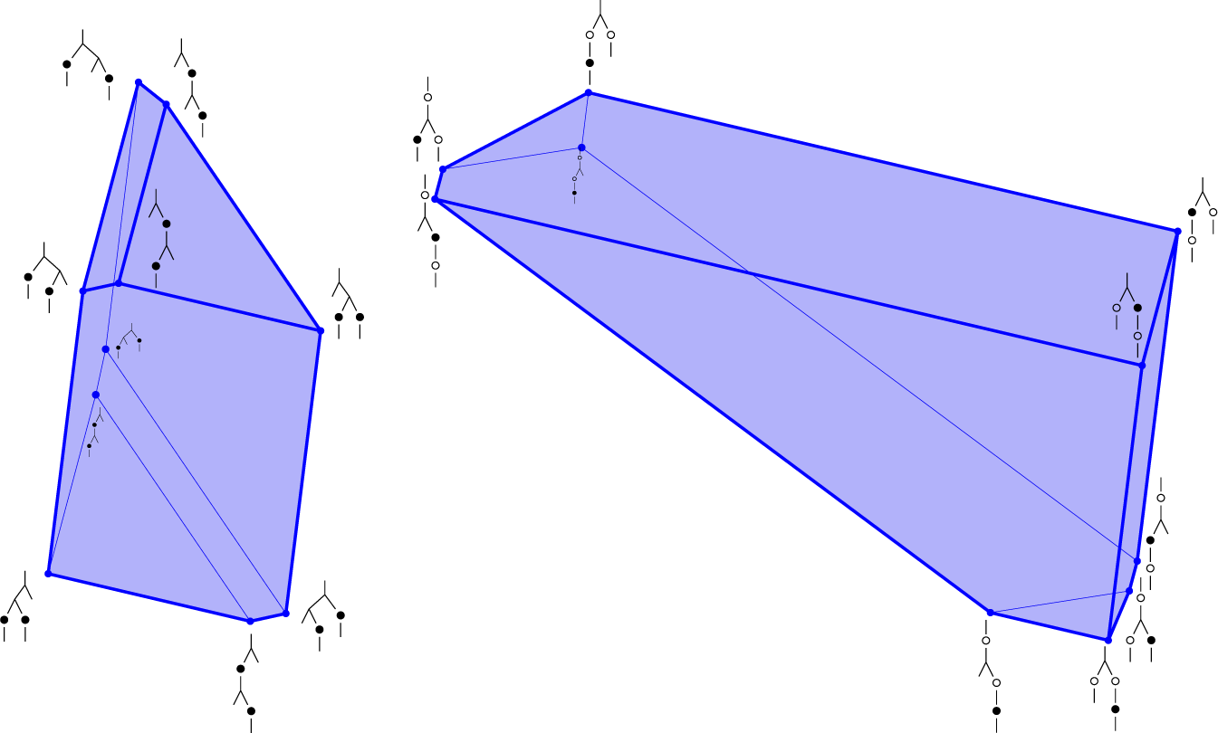
Figure 14 illustrates polytopal realizations of the pebble tree fans  and
 . Note that, while they have the same combinatorics by Proposition 2.10, their geometric realizations differ.
The pebble tree polytopes  (left) and
 (right).

Figure 14: Long description
The diagram consists of two panels.
Left panel: A three-dimensional blue translucent polytope, P T P super 0, 1 sub 3, with a tall, irregular prismatic shape. It has several vertices and edges highlighted in dark blue. Surrounding the polytope are eight tree diagrams acting as labels for specific vertices. These trees consist of branching lines with black circular nodes. The trees vary in their branching structure, representing different combinatorial states of the pebble tree.
Right panel: A wider, more elongated blue translucent polytope, P T P super 1, 1 sub 2. This shape is more flattened and stretched horizontally compared to the first. It is surrounded by ten tree diagram labels. These labels are more complex than the first panel, featuring both solid black nodes and hollow white nodes on the branching structures. The labels are positioned around the perimeter of the polytope, corresponding to its various vertices and facets.
Finally, we translate the first three points of Proposition 2.10 and Remark 2.11 to pebble tree polytopes. Note that the last two transformations of Proposition 2.10 do not respect the geometry of the pebble tree polytopes.
Proposition 3.11 Consider the operations of Definitions 2.2–2.4.
-
(1) The map defined by ${\boldsymbol {e}}_{\ell j + i - \delta _{j \ne 0}} \mapsto {\boldsymbol {e}}_{\ell (j + 1) - i}$
for any
$(i,j) \in ([\ell ] \times [0,b+u]) \smallsetminus \{(\ell ,0)\}$
induces an isometry of the pebble tree polytope . -
(2) If $u> 1$
, the pebble tree polytope is a facet of the pebble tree polytope . Hence, is a codimension u face of . -
(3) The pebble tree polytope
is a codimension
$\ell $
face of the pebble tree polytope where
$h(X) = h'(\left \{ x+1 \;\middle |\; x \in X \right \})$
for
$X \subseteq [b+u]$
.


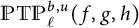 .

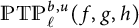 is a facet of the pebble tree polytope
 . Hence,
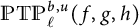 is a codimension u face of
 .
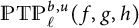 is a codimension

 where


Remark 3.12 Following Remarks 2.5, 2.11, and 2.18, observe that for any signature  , the
$\alpha $
 -assocoipahedron of [Reference Poirier and TradlerPT18] is realized by a face of the pebble tree polytope
 . For instance, Figure 15 shows faces of the pebble tree polytopes
 and
 which realize the
$\alpha $
 -assocoipahedra for
 and
 presented in [Reference Poirier and TradlerPT18, Figures 8, 9, 14, and 15]. Note that the combinatorics of the
 -assocoipahedra represented in Figure 15 (right) is also isomorphic to the pebble tree polytopes
 represented in Figure 14 by combining Points (2) and (4) of Proposition 2.17.
The
$\alpha $
 -assocoipahedra for
 (left) and
 (right), realized as faces of the pebble tree polytopes
 and
 .

Figure 15: Long description
Two panels show geometric realizations of P T P super 1, 0 sub 4 and P T P super 1, 0 sub 3.
Left Panel: A complex blue translucent polytope with multiple facets. It is the alpha-assocoipahedra for alpha equals O I I O I. Small black tree diagrams are positioned near each vertex. Starting from the top and moving clockwise, the trees show varying branching structures with black dots representing nodes. Some trees are simple vertical lines with two dots, while others are more complex with multiple bifurcations and up to five dots.
Right Panel: A simpler blue translucent polytope representing alpha equals O O O I. It has fewer vertices and larger facets compared to the left panel. Similar tree diagrams are anchored to its vertices. The trees on this side generally appear less complex, with many consisting of a single main stem and one or two branches, reflecting the different alpha value. Both polytopes use blue lines for edges and lighter blue shading for faces to indicate three-dimensional volume.
4 Pebble tree numerology
In this section, we compute the generating functions of the maximal pebble trees (Section 4.1) and of all the pebble trees (Section 4.2), and gather explicit expansions of these generating functions (Section 4.3). While the methods are standard computations based on generatingfunctionology [Reference Flajolet and SedgewickFS09], the results reveal a few surprises. All references like A000108 are entries of the Online Encyclopedia of Integer Sequences [OEI10].
4.1 Enumeration of maximal pebble trees
We start with the enumeration of the maximal pebble trees which is significantly simpler.
Definition 4.1 For
$\ell , u, b \in \mathbb {N}$
 , we denote by
$m_\ell ^{b,u}$
 the number of maximal pebble trees of
 (i.e., with
$\ell $
 leaves, b balanced and u unbalanced colors). We consider the generating function

Proposition 4.1 The generating functions  satisfy the functional equations

where
$\delta $
 is the Kronecker delta. Hence,
 is algebraic for any
$b,u \in \mathbb {N}$
 .
Proof A maximal pebble tree in  is:
-
• either a leaf if $s = t$
and
$B = \varnothing $
, -
• or a unary node with a single pebble colored by
and a child in , -
• or a binary node with no pebble and two children in
and for some
$r \in [s,t]$
and
$V \subseteq U$
.


 and a child in
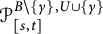 ,
 and
 for some


The functional equations for  are immediate consequences of this structural decomposition by classical generatingfunctionology [Reference Flajolet and SedgewickFS09]. The algebraicity of
 follows as it belongs to a system of finitely many polynomial equations (all equations for a given sum
$b+u$
 ).
Example 4.2 When
$b = u = 0$
 , we recover the functional equation
${\mathfrak{M}^{0,0}(x)=x+\mathfrak{M}^{0,0}(x)^{2}}$
 which yields the classical Catalan generating function

Example 4.3 For
$b + u = 1$
 , we obtain that

from which we can compute the expansions

These functions actually both satisfy a cubic equation, namely

Example 4.4 For
$b + u = 2$
 , we obtain


From which we can compute the expansions:

The expansion of  is quite surprising, but can be explained by a tiny functional miracle. Indeed, observe that we obtain that
 from Equation (4.1) and that
 from Equation (4.2). Replacing
 on both sides of Equation (4.3), we obtain

This shows that
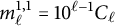
$m_\ell ^{1,1} = 10^{\ell -1} C_\ell $
 , where
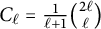
$C_\ell = \frac {1}{\ell +1} \binom {2\ell }{\ell }$
 is the Catalan number.
Consider the map sending a maximal pebble tree of  to its underlying binary tree. In view of the formula
${m_\ell ^{1,1} = 10^{\ell -1} C_\ell }$
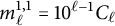 , it is natural to expect that its fibers all have size
$10^{\ell -1}$
 . However, while the size of the fiber of a binary tree T is clearly invariant under reordering the children of T, it is not constant on all binary trees already for
$\ell = 4$
 . Namely, the fiber of the binary tree whose children are both the tree on
$2$
 leaves contains
$968$
 pebble trees of
 , while the fiber of each of the remaining
$4$
 binary trees on
$4$
 leaves contains
$1008$
 pebble trees of
 .
Despite this disappointing observation, one can provide a bijective explanation for the appearance of the Catalan numbers in
$m_\ell ^{1,1}$
 . It requires the following observation.

Long description
The image contains a block of text on the left and two tree diagrams on the right.
Text content:
Any maximal white-circle-balanced black-circle-unbalanced pebble tree can be uniquely obtained from a right comb by attaching
* to each left leaf, a maximal {white-circle, black-circle}-balanced pebble tree,
* to the right leaf, a maximal white-circle-balanced black-circle-unbalanced pebble tree, whose root is
- either a unary node with a white-circle pebble, whose unique child X is {white-circle, black-circle}-unbalanced,
- or a binary node with no pebble, whose left child Y is white-circle-balanced black-circle-unbalanced and whose right child Z is {white-circle, black-circle}-balanced.
These two options are illustrated on the right. A similar decomposition holds with a left comb instead of a right comb.
Diagrams:
* Top diagram: A tree with a main spine sloping down to the right. Left-branching leaves are labeled T sub 1 through T sub k. The spine terminates at a node with a white circle pebble, which has a single vertical child labeled X.
* Bottom diagram: A similar tree with a main spine sloping down to the right. Left-branching leaves are labeled T sub 1 through T sub k. The spine terminates at a binary branching node with no pebble, which splits into a left child Y and a right child Z.
We now proceed to define, for
$\ell , r \ge 1$
 , an explicit bijection
$\psi $
 sending a triple
$(T, L, R)$
 of maximal pebble trees of
 ,
 , and
 respectively to a maximal pebble tree of
 . The image
$\psi (T, L, R)$
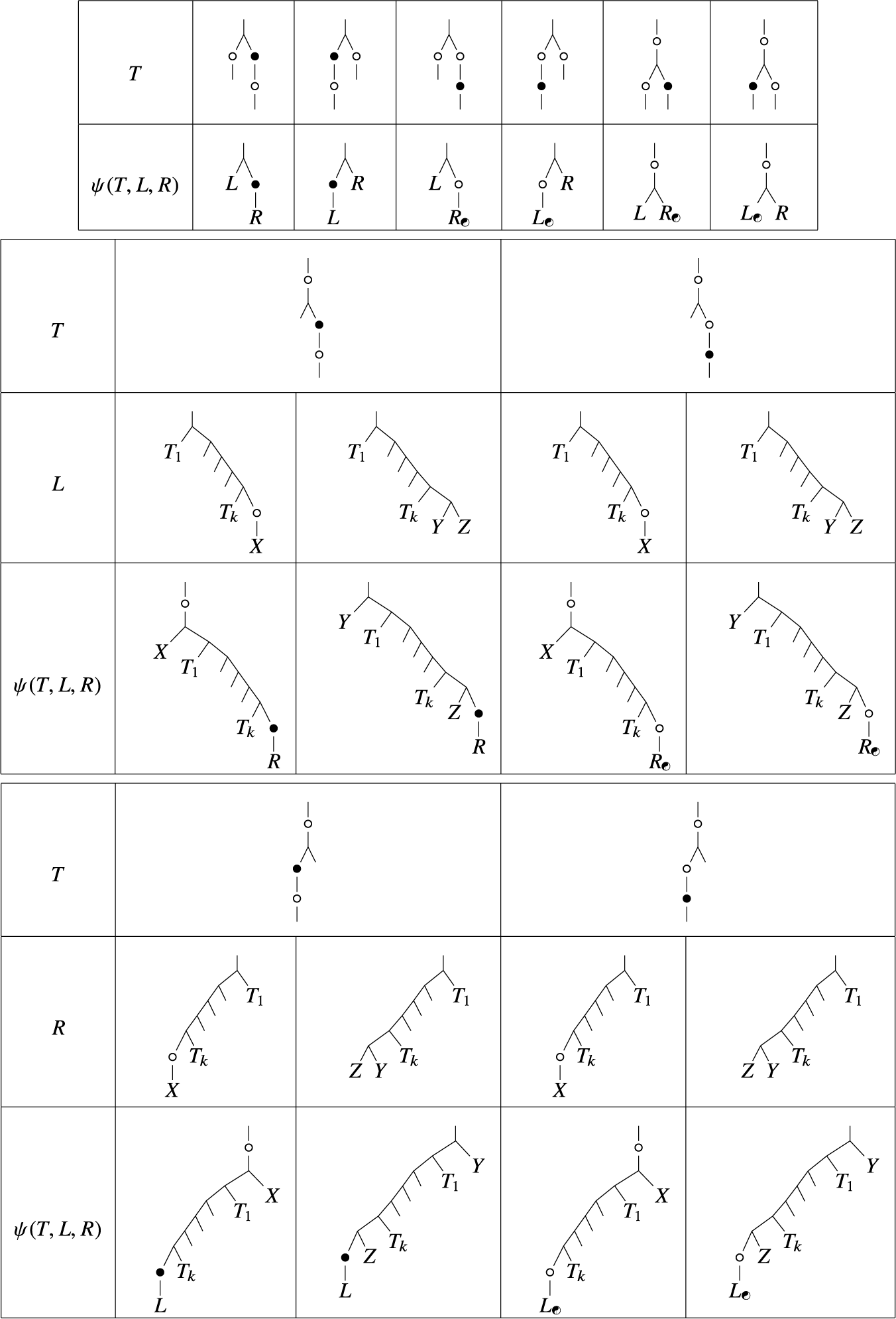
 is described in Figure 16. Note that
$\psi (T, L, R)$
 sometimes depends on the type of L or R in the sense of the decomposition of Remark 4.5. In this description, we denote by
 the
$\bullet $
 -balanced
$\circ $
 -unbalanced pebble tree obtained by exchanging the
$\circ $
 and
$\bullet $
 pebbles in a
$\circ $
 -balanced
$\bullet $
 -unbalanced pebble tree T. As the decomposition of Remark 4.5 is unique, the map
$\psi $
 is well defined, and it is immediate to check that the resulting trees are maximal pebble trees of
 . Again by Remark 4.5, it is straightforward to check that
$\psi $
 is bijective. Finally, as
$m_2^{1,1} = 10$
 , the existence of the bijection
$\psi $
 directly implies Equation (4.4), hence the fact that
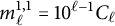
${m_\ell ^{1,1} = 10^{\ell -1} C_\ell }$
 .
Bijection
$\psi $
 sending a triple
$(T, L, R)$
 of maximal pebble trees of
 ,
 and
 respectively to a maximal pebble tree of
 .

Figure 16: Long description
The diagram consists of three horizontal tables.
Top Table: Contains two rows. The first row, labeled T, shows six small tree configurations with open and closed circles (pebbles) at different nodes. The second row, labeled psi (T, L, R), shows the corresponding output trees where L and R are attached as subtrees to the nodes of T based on the pebble positions.
Middle Table: Focuses on cases where L is a larger tree structure. It has three rows: T, L, and psi (T, L, R).
- The T row shows two specific tree configurations.
- The L row shows four variations of a right-leaning comb-like tree structure with nodes labeled T sub 1 through T sub k, and terminal nodes X, Y, or Z.
- The psi (T, L, R) row shows the resulting complex trees where the L structure is integrated into the T framework, often with R attached at the bottom right.
Bottom Table: Focuses on cases where R is a larger tree structure. It has three rows: T, R, and psi (T, L, R).
- The T row shows two tree configurations.
- The R row shows four variations of a left-leaning comb-like tree structure with nodes labeled T sub 1 through T sub k, and terminal nodes X, Y, or Z.
- The psi (T, L, R) row shows the resulting complex trees where the R structure is integrated into the T framework, with L attached at the bottom left.
Throughout the diagram, open circles represent empty pebble slots and solid black circles represent filled pebble slots, determining the grafting points for the bijection.
4.2 Enumeration of all pebble trees
We now consider all pebble trees.
Definition 4.2 For
$\ell , n, u, b \in \mathbb {N}$
 , we denote by
$p_{\ell ,n}^{b,u}$
 the number of pebble tree with
$\ell $
 leaves, n nodes, b balanced and u unbalanced colors. We consider the generating function

Proposition 4.6 The generating functions  satisfy the functional equations

where
$\delta $
 is the Kronecker delta, where each
$X_i$
 ranges among arbitrary subsets of
$[d]$
 while each
$Y_j$
 ranges among strict subsets of
$[d]$
 , and where
 and
 for any
$k \in [d]$
 . Hence,
 is algebraic for any
$b,u \in \mathbb {N}$
 .
Proof A pebble tree of  is:
-
• either a leaf if $s = t$
and
$B = \varnothing $
, -
• or a unary node with some pebbles colored by a non-empty subset $S \subseteq B$
(one pebble of each color in S) and a child in , -
• or a node with some pebbles and $d \ge 2$
children in respectively, for some
$s = s_1 \le t_1 = s_2 \le \dots \le t_d = t$
and
$B_i \subseteq B$
and
$U_i \subseteq U$
for all
$i \in [d]$
, such that
$\bigcap _{i \in [d]} U_i = \varnothing $
.


 ,

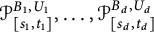 respectively, for some




The functional equations for  are immediate consequences of this structural decomposition by classical generatingfunctionology [Reference Flajolet and SedgewickFS09]. The algebraicity of
 follows as it belongs to a system of finitely many polynomial equations (all equations for a given sum
$b+u$
 ).
Example 4.7 When
$b = u = 0$
 , we recover the functional equation

which yield the classical Schröder generating function

The expansions of the generating functions  and
 for
$b + u \le 2$
 can be found in Section 4.3. Finally, we observe that the evaluations of
 at
$y = 1$
 and
$y = -1$
 have a geometric meaning.
Proposition 4.8 For any
$b,u \in \mathbb {N}$
 , the evaluation
 is the generating function of the total number of faces of the pebble tree polytope
 , and

Proof By Theorem 3.8,
$p_{\ell ,n}^{b,u}$
 is the number of
$(\ell + \ell b + \ell u - u - 2 - n)$
 -dimensional faces of the
$(\ell + \ell b + \ell u - u - 2)$
 -dimensional pebble tree polytope
 . This implies that
-
• $\sum _n p_{\ell ,n}^{b,u}$
is the total number of faces of , -
• $\sum _n p_{\ell ,n}^{b,u} (-1)^n = (-1)^{\ell + \ell b + \ell u - u - 2}$
by Euler’s formula.

 ,

This immediately implies the statement.
4.3 Expansions of generating functions
Below are the expansions of the generating functions  ,
 and
 of Definitions 4.1 and 4.2 for all
$b + u \le 2$
 .
$\underline {b = 0 \text { and } u = 0}$
 .

$\underline {b = 1 \text { and } u = 0.}$


$\underline {b = 0 \text { and } u = 1.}$


$\underline {b = 2 \text { and } u = 0.}$


$\underline {b = 1 \text { and } u = 1.}$


$\underline {b = 0 \text { and } u = 2.}$


Acknowledgements
I am grateful to Doriann Albertin for discussions around Example 4.4 and for a very constructive proofreading, to Wenjie Fang for pointing out Remark 2.6 and for discussions on Propositions 4.1 and 4.6, to Guillaume Laplante-Anfossi for motivating me to find polytopal realizations of the assocoipahedra, to Thibaut Mazuir for algebraic discussions on the assocoipahedra, and to Anna de Mier, Jordi Castellví Foguet and Clément Requilé for discussions on Example 4.4 during the 3rd Workshop on Geometric, Algebraic and Probabilistic Combinatorics in Monserrat on July 2022. Finally, I am grateful to an anonymous referee for useful suggestions on the presentation of this paper. This research benefited from computations and tests done using the open-source mathematical software Sage [Sd16] and its combinatorics features developed by the Sage-combinat community [SCc16], and from the Online Encyclopedia of Integer Sequences [OEI10].






















 Open access

