Implications
The commercial application of genomic selection implies that relatively large numbers of important breeding animals are genotyped using high-density markers. This opens up the possibility to perform quantitative trait loci (QTL)-mapping studies with greater power and precision than was possible beforehand, while the estimated SNP effects are valid for the whole evaluated population rather than, for instance, only within a sire family. Some of the models applied for genomic breeding value prediction find their origin in QTL mapping. For instance, the internal model (or rather single-nucleotide polymorphisms (SNP)) selection step in BayesB, in fact assesses the probability that a SNP is linked to a QTL. This implies that applying such models, as a ‘by-product’ yield the probability that QTL exist across the genome. Although QTL mapping in itself is not the primary goal, identification of regions that heavily influence a number of traits, would greatly help to further disentangle the nature of different traits, as well as the genetic correlation between them.
Introduction
An important tool in genetic improvement of livestock species is the prediction of breeding values. Breeding value prediction depends on knowledge of relationships between individuals. Defining genetic relationships between animals allows estimation of the proportion of phenotypic variance that is heritable. A major breakthrough in animal breeding was the application of best linear unbiased prediction (BLUP) to predict breeding values, made possible by direct derivation of the inverse additive relationship matrix (Henderson, Reference Henderson1975). Three disadvantages from applying this method to predict breeding values are the following: (i) to estimate reliable breeding values for selection candidates, phenotypic information of the animal itself or close relatives is needed; (ii) BLUP favours close relatives leading to increased inbreeding; and (iii) the infinitesimal model is assumed, meaning that an infinite number of genes with small effect underlie a trait. Efforts to apply quantitative trait loci (QTL) mapping, to allow implementation of marker-assisted selection (MAS), tried to tackle both issues (Dekkers and Hospital, Reference Dekkers and Hospital2002). These approaches identify QTL that have a large effect on a trait and trace those to enhance reliability of predicted breeding values, before phenotypic information is available.
Early applications of QTL mapping have the disadvantage that still phenotypic records are needed from the animals themselves or from their close relatives, because they use linkage mapping, where the linkage phase between marker and QTL has to be estimated for instance for each (grand) sire family (e.g. Weller et al., Reference Weller, Kashi and Soller1990). More recent developed methods of QTL mapping rely on population-wide linkage disequilibrium (LD) information. This means that in the model it is assumed that across the population each separate allele of a QTL locus generally is transmitted together with a separate allele at a marker locus. This assumption holds when recombination between a QTL and a marker is limited, that is, the physical distance between a marker and QTL locus that are in LD should be small and thus a high marker density is needed. With increasing distance between two loci that are in LD, the chance of recombination increases, and therefore, the accuracy of forward prediction using estimated single-nucleotide polymorphisms (SNP) effects decreases. The recent availability of high-throughput SNP genotyping provides dense marker maps at reasonably low cost, and allows to map more and smaller QTL. However, the effect of small QTL is hard to estimate, implying that the inaccuracy and bias of estimated QTL effects may increase.
Both the efficiency and the accuracy of detecting QTL can be increased by applying multiple QTL models (Jansen, Reference Jansen1993; Zeng, Reference Zeng1994). Meuwissen et al. (Reference Meuwissen, Hayes and Goddard2001) applied a multiple QTL model and skipped the QTL-mapping step in a method that is termed genomic selection. This method simultaneously estimates the effects for a large number of markers across the chromosome, for example, approximately 50 000 are currently applied in cattle (Van Tassell et al., Reference Van Tassell, Smith, Matukumalli, Taylor, Schnabel, Lawley, Haudenschild, Moore, Warren and Sonstegard2008), and directly sums those effects to total so-called genomic estimated breeding values (GEBVs). The fact that all effects are estimated simultaneously implies that, even though individual marker effects may be overestimated, the expected variance of the total estimated breeding values, including all estimated marker effects, does not exceed the total genetic variance.
The objective of this paper is to review the methods and procedures applied for genomic prediction, as well as the prediction of GEBVs and the accuracy of GEBVs.
Genomic prediction – the process
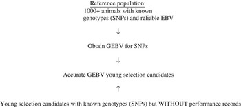
The key issue in genomic prediction is estimation of effects of individual SNP alleles on a trait of interest. These SNP effects are estimated using a reference population, also termed training data (Meuwissen, Reference Meuwissen2007) (Figure 1). This reference population typically comprises at least 1000 individuals that have reliable phenotypic as well as genotypic information. This phenotypic information could be own phenotypic performance, but also breeding values obtained from (national) evaluations based on phenotypic information (De Roos et al., Reference De Roos, Schrooten, Mullaart, Calus and Veerkamp2007; De Roos et al., Reference De Roos, Schrooten, Mullaart, Van der Beek, De Jong and Voskamp2009; Lund and Su, Reference Lund and Su2009), deregressed proofs (Berry et al., Reference Berry, Kearney and Harris2009; Schenkel et al., Reference Schenkel, Sargolzaei, Kistemaker, Jansen, Sullivan, Van Doormaal, VanRaden and Wiggans2009; VanRaden et al., Reference VanRaden, Van Tassell, Wiggans, Sonstegard, Schnabel, Taylor and Schenkel2009), daughter-yield deviations or average offspring performance (González-Recio et al., Reference González-Recio, Gianola, Long, Weigel, Rosa and Avendaño2008). By linking the genotypic and phenotypic information together, estimates for each of the SNPs are obtained. The last step in the process involves genotyping of young selection candidates, whose GEBVs are obtained by summing up all the relevant SNP effects.
Genomic selection – the process.

An important question is which animals need to be included in the reference population. Several approaches can be taken. In dairy cattle, for instance, the most straightforward approach is to use proven bulls (De Roos et al., Reference De Roos, Schrooten, Mullaart, Calus and Veerkamp2007; VanRaden et al., Reference VanRaden, Van Tassell, Wiggans, Sonstegard, Schnabel, Taylor and Schenkel2009), that have reliable national breeding values, which allows to derive reliable deregressed proofs. This approach is an obvious choice when obtaining reliable phenotypes is time consuming and expensive, compared with the cost of genotyping. Furthermore, the young selection candidates may be close relatives (such as offspring) of the phenotyped animals in the reference population, which may enhance the reliabilities of the breeding values (Habier et al., Reference Habier, Fernando and Dekkers2007). When animals for the reference population both need to be genotyped and phenotyped, and costs of phenotyping are low compared with genotyping costs, the design of the reference population may be optimized cost effectively. Although so far not much research is done on the optimal composition of a reference population, theoretically the optimal reference population should comprise the whole range of phenotypes and genotypes, to allow reliable prediction across these ranges. However, this is not possible in real life, so the reference population should be designed to reflect the whole range of phenotypes and genotypes as close as possible. Since prediction of GEBVs is shown to be more reliable when juvenile animals share their recent pedigree with animals in the reference population (Habier et al., Reference Habier, Fernando and Dekkers2007), it seems straightforward that composing a reference population closely related to the juvenile selection candidates is an optimal strategy. De Roos et al. (Reference De Roos, Hayes and Goddard2008a), however, showed, that it is particularly important that at least some of the animals in the reference population originate from the same pedigree or line as the juvenile animals. This indicates that a reference population that needs to serve multiple lines may optimally contain animals from all lines, and yield nearly as accurate predictions for each of the lines as a line-specific reference population may do. The likely reason for this is that combining animals from different families or lines ensures that only LD that persists across those families or lines is utilized in the prediction equations. This is, however, only possible if marker density is sufficiently high such that each QTL has at least one SNP that is in sufficiently high LD across multiple lines or breeds. De Roos et al. (Reference De Roos, Hayes, Spelman and Goddard2008b) showed that in order to accurately predict GEBVs for Jerseys, using prediction equations based on a Holstein–Friesian reference population, at least 300 000 SNPs are needed, while the current available SNPs (approximately 50 000) are sufficient for accurate predictions within the same breed. In addition, Harris et al. (Reference Harris, Johnson and Spelman2008) reported that based on 44 146 SNPs, GEBVs for Jerseys using SNP effects estimated in Holstein, and vice versa, were not accurately predicted. Since within the Holstein–Friesian breed, the average r 2 between adjacent SNPs at a marker density that resembles the currently used 50 000 SNPs is between 0.15 and 0.20 (De Roos et al., Reference De Roos, Hayes, Spelman and Goddard2008b; Khatkar et al., Reference Khatkar, Nicholas, Collins, Zenger, Al Cavanagh, Barris, Schnabel, Taylor and Raadsma2008), it is expected that panels that may be used to predict breeding values across breeds or lines should capture at least the same level of LD across those breeds or lines.
Genome – wide breeding value estimation
Sources of data
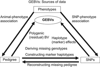
In terms of sources of information, the simplest model to predict GEBVs only uses phenotypic and genotypic data (e.g. Meuwissen et al., Reference Meuwissen, Hayes and Goddard2001), where genotypic data in recent commercial applications nearly always consist of SNP genotypes. In addition, pedigree data may be used (Figure 2). This allows to derive an additive relationship matrix and incorporation of polygenic breeding values in the model (Calus and Veerkamp, Reference Calus and Veerkamp2007). Whenever pedigree information is not available, the additive relationship matrix can be constructed directly from the genotypic information (e.g. Fernando, Reference Fernando1998). In terms of pre-processing data, pedigree information can be compared with SNP information to discover possible genotype or pedigree errors, while pedigree and SNP information may be used jointly to derive marker haplotypes (e.g. Meuwissen and Goddard, Reference Meuwissen and Goddard2001).
Sources of data that may be used in genome-wide prediction of breeding values.

The model
Generally, the model to predict GEBVs, considering only additive genetic effects, is described as:

where yi may be a phenotype, national EBV, daughter-yield deviation, deregressed EBV or average offspring performance of animal i; fixed effects are a set of fixed effects, which may only be the overall mean, animali is a polygenic effect, Σ(SNPijk) is the sum of both SNP effects (k = 1, 2), summed across all loci (j) for animal i. Note that for both alleles, a separate effect may be estimated (k = 1, 2), or alternatively, one allele substitution effect a may be estimated per locus.
The GEBVs of animal i can be obtained as follows:

Parameterization of the model
The simplest parameterization of the model consists of estimating effects for each SNP allele, or estimating allele substitution effects for each SNP locus (e.g. Xu, Reference Xu2003b). This implies that both the order of the SNPs along the genome and the linkage phase of the SNP alleles do not need to be known. A disadvantage of fitting the SNP alleles is that the model ignores the effect of recombination, which may change the linkage between marker and QTL alleles. Estimating effects of constructed marker haplotypes solves this problem to some extent: copies of each unique haplotype are assumed to carry the same QTL alleles. In this case, the marker haplotypes are treated to be alike-in-state (AIS; e.g. Meuwissen et al., Reference Meuwissen, Hayes and Goddard2001; Villumsen and Janss, Reference Villumsen and Janss2008).
The assumption that copies of each unique haplotype carry the same QTL allele can be relaxed by treating haplotypes to be identical-by-descent (IBD; Meuwissen and Goddard, Reference Meuwissen and Goddard2001). Two haplotypes are IBD whenever they consist of the same marker alleles due to inheritance from a common ancestor. Since the probability that two haplotypes are IBD is nearly always larger than zero and smaller than one, predicted IBD probabilities between haplotypes are included in the model to account for the relationships between haplotypes (Meuwissen and Goddard, Reference Meuwissen and Goddard2001). An additional difference between marker AIS and IBD haplotypes is that the IBD status of haplotypes is evaluated at one position in the genome (a so-called putative QTL position), whereas AIS haplotypes are considered to be AIS across the whole haplotype. When IBD probabilities between two haplotypes are close to one, those haplotypes are usually considered to be the same to reduce the number of effects that needs to be estimated and thereby increasing power to estimate effects (Yu et al., Reference Yu, Xu, Rao and Province2005) and speeding up convergence (Calus et al., Reference Calus, Meuwissen, Windig, Knol, Schrooten, Vereijken and Veerkamp2009).
Underlying QTL distribution
Estimated SNP or haplotype effects capture at least partly the underlying QTL effects. Consequently, the distribution of estimated SNP or haplotype effects should resemble the distribution of the underlying QTL effects. Estimated distributions of QTL effects suggest that there are many loci of small (near zero) effect and that there are few loci with large effect (Hayes and Goddard, Reference Hayes and Goddard2001). However, for many traits, the distribution of underlying QTL may largely be unknown a priori. The design of QTL-mapping studies may lead to overestimated effects for large QTL (Xu, Reference Xu2003a), while small QTL may not be picked up at all. Furthermore, the effect of a single QTL may be explained by multiple SNPs, leading to more SNP supposedly linked to QTL, on average having relatively smaller effects than the QTL. This suggests that prior information on the distribution of QTL effects should be used with caution when designing models to estimate SNP effects, or, alternatively, that models should be able to make inferences from the data with regard to the distribution of QTL effects.
Methods to solve the model
The main challenge for models that estimate SNP effects is that generally phenotypes are available from a few thousand animals, while the number of SNP is much larger, for instance, approximately 50 000 SNPs for cattle. A practical problem is how this set of equations can be solved. Another issue is that the distribution of QTL effects implies that there are many loci of small (near zero) effect and that there are few loci with large effect (Hayes and Goddard, Reference Hayes and Goddard2001). This implies that methods may have to be able to eliminate loci with (near) zero effect and/or have to be able to deal with the problem that the number of loci whose effect need to be estimated, is much larger than the number of records available. A straightforward approach is to select a reduced set of explaining loci. This can be done by just looking at the genomic variation, that is, by selecting a subset of SNPs (so-called tag-SNPs), that together explain a large part of the genomic variation in the full set of SNPs (e.g. Ke and Cardon, Reference Ke and Cardon2003). Another approach is to select a subset of SNPs that may be associated with a phenotype of interest. Applied approaches are, for instance, machine learning classification procedures (Long et al., Reference Long, Gianola, Rosa, Weigel and Avendaño2007), or forward stepwise regression to determine for each SNP whether it significantly explains phenotypic variance, given the effects of the already selected SNPs (Habier et al., Reference Habier, Fernando and Dekkers2007).
Conceptually more appealing is to incorporate a step in the model that determines for each of the SNPs whether it is associated with a QTL or not, and therefore, whether it has a non-zero effect on the phenotype or not. Such an approach was implemented in a Bayesian model by Meuwissen et al. (Reference Meuwissen, Hayes and Goddard2001), and termed BayesB. In BayesB, a Metropolis–Hastings step is used in every iteration to determine for each locus whether it has an effect on the phenotype or not. If it has not, the effect of that locus is set to zero. One concern about this model is that it relies quite heavily on the considered prior information to infer the SNP effects (Gianola et al., Reference Gianola, Fernando and Stella2006).
An alternative approach is to apply a mixture model, where one distribution of variances is assumed for loci with an association with the phenotype, and a distribution with very small values is assumed for loci with no association with the phenotype (Meuwissen and Goddard, Reference Meuwissen and Goddard2004; Calus et al., Reference Calus, Meuwissen, De Roos and Veerkamp2008; Janss et al., Reference Janss, Gregersen, Bendixen and Lund2008). This method allows to apply Gibbs sampling, while avoiding the Metropolis–Hastings step that is used in BayesB. The benefit of this method is that all loci for which no clear evidence is found for a direct association, together still may explain a substantial part of the genetic variance (Calus et al., Reference Calus, Meuwissen, De Roos and Veerkamp2008). This makes that these mixture models are able to combine the properties of the BayesB and the ‘genomic BLUP’ (GBLUP) model; the distribution with large effects is expected to pick up the same SNPs as the BayesB model, while the other SNPs still all explain a roughly equal small amount of the variance as in the GBLUP model. The GBLUP model assumes that each of the SNPs equally contributes to the additive genetic variance (Meuwissen et al., Reference Meuwissen, Hayes and Goddard2001). It has been shown that constructing a genomic relationship matrix based on all markers and included in a regular mixed model, instead of a pedigree-based relationship matrix, is equivalent to the GBLUP method (Goddard, Reference Goddard2009). The contribution of each locus to the genomic relationship matrix can be weighted to account for different variances per locus or differences in local marker density (VanRaden, Reference VanRaden2008).
Several other models have been considered for genome-wide prediction. Apart from a few methods that assume equal contribution to the genetic variance by all loci, a common feature of these methods is to reduce the dimension of the SNP data. Reported alternatives include non-parametric kernel methods (Gianola et al., Reference Gianola, Fernando and Stella2006; Bennewitz and Meuwissen, Reference Bennewitz and Meuwissen2008; Gianola and van Kaam, Reference Gianola and van Kaam2008), partial least squares (PLS) regression (Raadsma et al., Reference Raadsma, Moser, Crump, Khatkar, Zenger, Cavanagh, Hawken, Sölkner and Tier2008; Solberg, Reference Solberg2008), principal component analysis (PCA; Solberg, Reference Solberg2008), genetic algorithms, and Bayesian LASSO (de los Campos et al., Reference de los Campos, Naya, Gianola, Crossa, Legarra, Manfredi, Weigel and Cotes2009). Kernel methods were shown to yield similar results as the Bayesian methods for purely additive models (Bennewitz and Meuwissen, Reference Bennewitz and Meuwissen2008), but may outperform the Bayesian models when considering non-additive effects (González-Recio et al., Reference González-Recio, Gianola, Long, Weigel, Rosa and Avendaño2008). PCA reduces dimensionality of the SNP data matrix by finding a few variables explaining as much variance as possible, while PLS does the same, yet conditional on the dependent variable (i.e. the phenotypic information).
Nearly all of the mentioned studies only considered additive genetic effects in the model. Some models have been presented that explicitly include dominance (Xu, Reference Xu2003b) or epistatic effects (Xu and Jia, Reference Xu and Jia2007). The main problem with the epistatic effects is that for a high number of markers the number of potential interactions becomes unreasonably high, and evaluating all of them is impossible. A suggested solution involves modelling one genetic term that includes additive and epistatic effects, without discriminating explicitly between them (Gianola et al., Reference Gianola, Fernando and Stella2006; Gianola and van Kaam, Reference Gianola and van Kaam2008).
Accuracies of GEBVs
Results from simulation studies
In the following, the term accuracy is used for the correlation between true and estimated breeding values, usually denoted as rTI . The accuracy of GEBV depends partly on the parameterization of the model and the statistical model that is used to solve it. Comparisons, based on simulated data, indicated that at low marker density the IBD-haplotype parameterization yielded considerable higher accuracy followed by the IBS-haplotype parameterization and the single SNP model (Calus et al., Reference Calus, Meuwissen, De Roos and Veerkamp2008). At high marker density, with LD comparable to the marker density of commercially available SNP chips, the differences in accuracy between the models were negligible (Calus et al., Reference Calus, Meuwissen, De Roos and Veerkamp2008). Including a polygenic effect in the model also increased the accuracy of GEBVs at low marker density (Calus and Veerkamp, Reference Calus and Veerkamp2007), while at high marker density, or in a situation where the markers already explained most of the genetic variance, including a polygenic effect, hardly increased the accuracy of the GEBVs (Calus and Veerkamp, Reference Calus and Veerkamp2007; Solberg, Reference Solberg2008).
In simulation studies, Bayesian models, including BayesB and mixture models, have been reported to yield accuracies for animals without phenotypic records ranging from 0.7 to 0.8, when the marker density was equivalent to one SNP per cM and approximately 1000 animals were included in the reference population (Meuwissen et al., Reference Meuwissen, Hayes and Goddard2001; Habier et al., Reference Habier, Fernando and Dekkers2007; Calus et al., Reference Calus, Meuwissen, De Roos and Veerkamp2008; Solberg et al., Reference Solberg, Sonesson, Woolliams and Meuwissen2008). In these studies, the simulated QTL followed a gamma (Meuwissen et al., Reference Meuwissen, Hayes and Goddard2001; Calus et al., Reference Calus, Meuwissen, De Roos and Veerkamp2008; Solberg et al., Reference Solberg, Sonesson, Woolliams and Meuwissen2008) or normal distribution (Habier et al., Reference Habier, Fernando and Dekkers2007). Both distributions imply that a limited number of loci explains a large amount of the genetic variance, which fits the assumption of those Bayesian models. When the number of QTL (8700) was large relative to the number of markers (8729), a model that assumed equal contribution to the additive variance by each SNP (i.e. including a genomic relationship matrix instead of a pedigree-based relationship matrix) was shown to need at least 5000 (out of 8729) markers across the genome to give an accurate prediction of the simulated heritability (Hayes and Goddard, Reference Hayes and Goddard2008). These results suggest that fine-tuning the model depending on the trait and the underlying QTL distribution greatly adds to the fit of the model to the data.
Results based on real data
In applications to real dairy cattle data, allowing unequal contributions of SNPs to the genetic variance yielded GEBVs that had only a slightly higher reliability than GEBVs estimated with a model that assumed equal contributions of SNPs to the genetic variance (Hayes et al., Reference Hayes, Bowman, Chamberlain and Goddard2009; VanRaden et al., Reference VanRaden, Van Tassell, Wiggans, Sonstegard, Schnabel, Taylor and Schenkel2009). Reliabilities were, however, substantially higher using BayesB for traits that are affected by DGAT (VanRaden et al., Reference VanRaden, Van Tassell, Wiggans, Sonstegard, Schnabel, Taylor and Schenkel2009). These results suggest that the distribution of QTL effects in real data is generally less extreme than assumed in the above-mentioned simulation studies, but more research is needed to verify this.
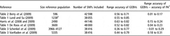
Table 1 gives a summary of ranges of GEBV accuracies for several dairy cattle breeding traits obtained from published studies based on real data with approximately 40 000 SNPs. Dairy cattle was used here as an example, because the results published on other species are limited so far. The accuracies from the different studies in Table 1 were obtained using different methods, apply for different groups of animals and may be for GEBVs or GEBVs blended with traditional proofs. Here, accuracies were used that were obtained for blended proofs of young bulls, or attempted to resemble those, whenever available. All studies presented in Table 1 showed that the accuracy of GEBVs was up to 0.31 higher than for pedigree indexes for bulls without any phenotypic data on offspring available, although for some traits, the GEBVs did not outperform pedigree indexes. Although inclusion of many different traits and use of different methods to assess the accuracy in different studies makes comparison of the obtained accuracies difficult, the reported maximum accuracy of each study was for a milk production trait. Those maximum values per study show that having 600 reference bulls resulted in lower accuracies (0.71) than when using at least 1200 reference bulls (accuracy ⩾0.77). Despite the limited number of studies in Table 1, and differences among the studies, the results suggest that there is a trend of increasing accuracy of GEBVs with increasing numbers of bulls in the reference population. Therefore, it seems advisable to include >1000 bulls in the reference population to obtain GEBVs for juvenile selection candidates with accuracies that are higher than those for pedigree indexes for all traits.
Ranges of accuracies for genomic estimated breeding values across traits as estimated in different countries for various sizes of the reference population

GEBVs = genomic estimated breeding values; PA = parent average.
1That is, pedigree index.
2Calculated as 80% of the reported 1548 bulls in the reference population.
Factors affecting the accuracy of GEBVs
Independent of the applied model to estimate marker effects, the accuracy of GEBVs strongly depends on the LD between marker and QTL loci that is consistent between the reference population and the animals for which GEBVs are predicted, and the accuracy of the estimated marker effects (Goddard, Reference Goddard2009). The accuracy of the estimated marker effects depends on the characteristics of the reference population, such as the number of included phenotypes (Hayes et al., Reference Hayes, Bowman, Chamberlain and Goddard2009; VanRaden et al., Reference VanRaden, Van Tassell, Wiggans, Sonstegard, Schnabel, Taylor and Schenkel2009), sampling of animals from the population (Habier et al., Reference Habier, Fernando and Dekkers2007) and the heritability of the trait (Calus et al., Reference Calus, Meuwissen, De Roos and Veerkamp2008; Hayes et al., Reference Hayes, Bowman, Chamberlain and Goddard2009). The ‘phenotypes’ of the reference population that are used to estimate the SNP effects may be deregressed EBVs, as applied in many cases for dairy bulls. In this case, the heritability is effectively increased per animal, by adjusting the residual variance by a weight that is calculated from the number of offspring contributing to the EBVs of the bull (e.g. Fikse and Banos, Reference Fikse and Banos2001). The LD between marker and QTL loci depends largely on the marker density. This indicates that the accuracy of GEBVs can be increased by increasing the number of animals in the reference population (Meuwissen et al., Reference Meuwissen, Hayes and Goddard2001), by sampling animals within families relevant for selection (Legarra et al., Reference Legarra, Robert-Granié, Manfredi and Elsen2008), by increasing the marker density (Meuwissen et al., Reference Meuwissen, Hayes and Goddard2001; Calus et al., Reference Calus, Meuwissen, De Roos and Veerkamp2008; Solberg et al., Reference Solberg, Sonesson, Woolliams and Meuwissen2008) and by increasing the heritability (Calus et al., Reference Calus, Meuwissen, De Roos and Veerkamp2008; Solberg, Reference Solberg2008).
The accuracy of prediction of GEBVs across and within different families or lines may be different, because the marker effects may absorb polygenic effects from one pedigree structure that are different from another structure (Habier et al., Reference Habier, Fernando and Dekkers2007; Legarra et al., Reference Legarra, Robert-Granié, Manfredi and Elsen2008). This does have a consequence not only for the construction of the reference population set, but also for the evaluation of different methods to predict GEBVs. An important additional parameter to compare different methods may therefore be the amount explained within and across family variance (Legarra and Misztal, Reference Legarra and Misztal2008).
Persistency of LD and accuracy of GEBVs across generations
Accurate genomic breeding value prediction strongly depends on the persistency of LD between markers and QTLs across generations. LD within a population can be created and maintained by selection, migration, mutation and drift (Lynch and Walsh, Reference Lynch and Walsh1998). The same forces may, however, decrease the LD between two loci, especially if the allele frequency at either locus is substantially changed. As a consequence, when marker effects are not re-estimated, the accuracy of GEBVs across generations is expected to decrease. In simulation studies, it was shown that the accuracy of GEBV decrease slowly when mating is random (Meuwissen et al., Reference Meuwissen, Hayes and Goddard2001; Solberg, Reference Solberg2008), and more rapid when selection is considered (Muir, Reference Muir2007). Since recombination will break up LD in both situations, this indicates that selection is an important factor to break up LD between markers and QTL.
The breakup of LD between markers and QTL, and consequently the reduction of accuracy of GEBVs across generations of selection, is one factor that determines the optimal frequency to re-estimate SNP effects. Another factor, from the perspective of the breeding program, is the frequency in which reliable phenotypes become available to re-estimate the SNP effects. In dairy cattle, a practical approach would be to continuously add phenotypic daughter information that becomes available for bulls that were selected as juveniles based on their GEBVs. In the time required to obtain this daughter information, two to three generations of selection maybe performed purely based on GEBVs (Villumsen et al., Reference Villumsen, Janss and Lund2009). Some studies showed that depending on the frequency of re-estimating the effects, different methods may be more suitable to obtain SNP effects whose accuracies are more persistent across generations. For instance, methods that are better able to disentangle between LD and linkage information show better persistency of GEBV accuracy across generations (Habier et al., Reference Habier, Fernando and Dekkers2007; Zhong et al., Reference Zhong, Dekkers, Fernando and Jannink2009). Despite the finding that approximately 50 000 SNPs are sufficient for within-breed genomic breeding value prediction in cattle, larger SNP arrays that undoubtedly will become available in the future will increase the LD between SNPs and QTL, leading to slower reduction of the accuracy of GEBVs across generations.
In most applications of genomic breeding value estimation, only additive genetic effects are considered. Despite this, a part of the estimated genetic effects may actually be non-additive by nature (Hill et al., Reference Hill, Goddard and Visscher2008). This may decrease the predictive ability of GEBVs across generations as well. For instance, in the situation that an epistatic effect between two unlinked loci is partially absorbed in the estimated additive effects due to extreme allele frequencies, the inheritance of this ‘additive’ effect will not follow the Mendelian rules. As a consequence, these fitted ‘additive’ effects may improve the fit of the model to the data, but actually decrease the accuracy of forward prediction.
Conclusions
Genomic selection is the ultimate application of markers in animal breeding. Using a reference population of animals with known genotypes and phenotypes enables to predict breeding values of young selection candidates that have reported accuracies that are up to 0.31 higher than those of pedigree indexes. Published results indicate that for dairy cattle at least approximately 1000 bulls are required in the reference population to obtain GEBVs with accuracies that compete with the accuracies of EBVs based on progeny testing for all traits. Several methods, of which most aim at reducing the dimension of the marker data, can be applied to estimate marker effects. The accuracy of genomic selection strongly depends on the characteristics of the reference population, as well as the relationship between the evaluated animals and the reference population. Breakup of LD between markers and QTL across generations advocates frequent re-estimation of marker effects to maintain the reliability of GEBVs at an acceptable level. Therefore, at low frequencies of re-estimating marker effects, it becomes more important that the model that estimates the marker effects capitalizes on LD information that is persistent across generations.
Acknowledgements
The author acknowledges the financial support of the Netherlands Organization for Scientific Research (NWO – Casimir), CRV and Hendrix Genetics. Two anonymous reviewers are thanked for useful and constructive comment on the manuscript.