I. INTRODUCTION
Shape memory alloys (SMAs) possess the ability to recover their original shape either after deformation (superelastic behavior) or through a postdeformation heating (shape memory effect) due to a reversible thermoelastic austenite–martensite phase transformation.Reference Otsuka and Wayman1 Among a wide variety of SMAs, the Ni–Ti (NiTi)-based ones are the most popular due to their attractive properties, such as low elastic anisotropy, high ductility, biocompatibility, high corrosion, and abrasion resistance.Reference Otsuka and Wayman1–Reference Rocher, El Medawar, Hornez, Traisnel, Breme and Hildebrand6 Therefore, they are either used or being considered for a wide variety of applications such as couplings, valves, actuators, and biomedical implants. In most of these applications, the SMA components are in the form of either thin wires or sheets or tubes. This smaller final size of the components means a fairly large number of thermomechanical processing steps become essential for breaking down of the large cast ingots to the required sizes. Also, hot deformation is an essential process for production of high-quality semifinished products of NiTi alloys.Reference Otsuka and Wayman1 Since the final microstructure controls the structural as well as functional properties and performance of SMAs, which are known to be sensitive to parameters such as grain size and texture, it becomes imperative to exercise careful control over the process parameters during high-temperature deformation. Extensive studies have been carried out about various thermomechanical treatment of NiTi alloys over the years.Reference Jean and Tsai7–Reference Paula, Mahesh, Santos, Fernandes and Viana15 Marked reduction in the tensile strength of NiTi alloys starts above 350 °C, whereas ductility starts rising at 550 °C, exceeding 100% at 630 °C. On this basis, it has been suggested that the optimum heating temperature for hot working of NiTi alloys is 800 °C.Reference Otsuka and Wayman1 However, few studies have been reported in literature about the deformation in NiTi alloy systemsReference Lin and Wu16–Reference Morakabati, Kheirandish, Aboutalebi, Karimi Taheri and Abbasi21 at high temperatures (above 800 °C). In particular, systematic scientific studies, which seek to identify the optimum combination of temperature and strain rate that yields a good microstructure postdeformation, have not yet been reported in open literature. In this article, we report such a study, wherein we use the processing maps approach to identify the hot working conditions for NiTiCu alloy, which is a widely used actuator alloy. The addition of Cu to NiTi has been extensively examined in literature in the view of improving shape memory and pseudoelastic characteristics.Reference Melton and Mercier22–Reference Lo, Wu and Horng27 Addition of Cu is effective for avoiding ageing effects, reduced compositional sensitivity of martensitic start temperature (Ms), reduced transformation hysteresis, and improving actuation response and fatigue properties.Reference Otsuka and Wayman1 Hence, NiTiCu alloys are attractive candidates for actuator applications.Reference Otsuka and Ren2, Reference Tang, Sandstrom, Wei and Miyazak28–Reference Grossmann, Frenzel, Samphath, Depka and Eggeler31
II. EXPERIMENTS
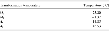
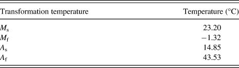
As cast Ni42Ti50Cu8 alloy (hereafter referred to as NiTiCu in the reminder of the text) was made by induction melting at 30-kg scale in a high-density graphite crucible and cast in a rectangular split graphite mould of 50 × 70 mm2 cross section under half atmosphere pressure argon gas after evacuation. High-purity Ni (99.99%), Cu (99.99%), and commercial purity ASTM 256 grade II Ti were used. The transformation temperatures of the alloy were obtained using differential scanning calorimetry (with scan rates of 10 °C/min). They are given in Table I. It is seen that the alloy is in the austenitic state at room temperature. Cylindrical specimens of 15-mm height and 10-mm diameter were used for the high-temperature uniaxial compression tests. Concentric circular grooves of 0.5 mm were made on the top and bottom surfaces of these specimens to help in retention of lubricant. High-temperature borosilicate lubricant was applied on the grooves to reduce the frictional stresses that were generated between the platens and the specimen during the deformation. In addition to this, a 1 mm and 45° chamfer was made at the corners of the cylindrical specimen to avoid foldover of the material during initial stages of compression testing. A hole of 0.8-mm diameter and 5-mm depth (i.e., halfway of the diameter of the cylindrical specimens) was drilled to attach a chromel/alumel thermocouple to the specimens. This thermocouple was used for measuring the specimen temperature directly.
Transformation temperatures of the NiTiCu alloy examined in this study.
The compression tests were performed on a servohydraulic machine with split furnace attached to it. The specimens, including the platens, remained covered by the furnace with four SiC heating elements. The temperature of the furnace chamber was measured by a thermocouple (platinum/platinum–rhodium), which extended up to the midway of the furnace. Temperature control of the furnace was accurate up to ± 2 °C. The compression tests were conducted at temperatures (T) of 800, 850, 900, 950, 1000, and 1050 °C. At each temperature, tests were conducted at constant true strain rates ( ) of 10−3, 10−2, 10−1, 10°, 101, and 102 s−1 to true strains of ∼0.7 (which corresponds to 50% deformation). Thus, a total of 36 tests were conducted.
Detailed microstructural analysis of the deformed samples was conducted on cross sections that were cut along the compression axis. It is well known that obtaining good quality optical micrographs of NiTi-based SMAs, especially those in the austenitic condition, is difficult. Therefore, electron backscatter diffraction (EBSD) was used to analyze the grain structure of each of these samples. The EBSD measurements were performed on FEI Quanta 3D FEG scanning electron microscope (FEI, Hillsboro, OR) using an orientation imaging microscopy (OIM; TexSEM Laboratories, Provo, UT) package. In each sample, an approximate area of about 0.3 × 0.9 mm2 was scanned with a step size of 0.5 μm. Care was taken to ensure that the beam and video conditions remained identical for all the scans. In EBSD analyses, a misorientation of 15° was used to represent high-angle grain boundaries and 2° was the limit to demarcate the grains by low-angle grain boundaries. The EBSD data obtained was further analyzed by using the OIM software to observe inverse pole figures, grain size, grain aspect ratio (GAR), and misorientation parameters.
III. RESULTS AND DISCUSSION
A. Stress–strain responses
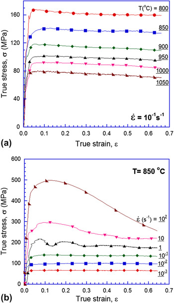
Figure 1 shows representative true stress–true strain curves obtained at a particular  [Fig. 1(a)] or temperature [Fig. 1(b)]. Note that the adiabatic correction factor is not yet accounted for in these plots. These plots show that the flow stress reduces with either a decrease in
 at a given T or with increasing T at a given
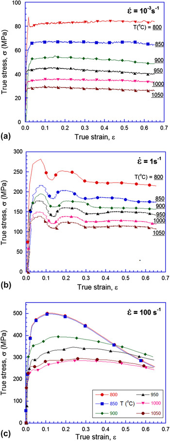
 . Figure 2 shows the response of the alloy at low, intermediate, and high values of
 . When
 is low, the alloy is essentially elastic-perfectly plastic, whereas at high strain rates marked flow softening beyond yield is observed. The latter is particularly prominent at low temperatures. At intermediate values of
 , the plastic flow was observed to be jerky in nature, similar to that reported in some Ti alloys.Reference Sen and Ramamurty32 The variations of yield stress with T and
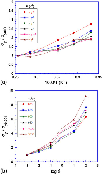
 are plotted in Figs. 3(a) and 3(b), respectively. Here, for comparison purposes the yield stress is normalized either with that obtained at 800 °C (at corresponding
 ) or with the yield stress obtained at a strain rate of 10−3 s−1 (at the corresponding T). The flow curves are monotonic in nature, i.e., the values of flow stress reduce with increasing T or decreasing
 (in all but 2 of the 36 points).
Representative true stress–true strain plots at (a) different temperatures and (b) different strain rates.

Representative true stress–true strain plots at (a) low, (b) intermediate, and (c) high strain rates. At low rates, the material behaves essentially as elastic-perfectly plastic, whereas marked flow softening is observed at high rates particularly at low temperatures. At intermediate strain rates, the flow is jerky in nature.

Variation of normalized yield stress with (a) temperature and (b) strain rate.

During plastic deformation, a temperature rise associated with flow softening due to heating could occur, particularly at high  , which needs to be taken into account. For the adiabatic correction, we have utilized the approach proposed by Goetz and SemiatinReference Goetz and Semiatin33 The change in temperature, ΔT, is measured with the help of the thermocouple attached to the specimen. The stress–strain data are corrected for adiabatic heating as,
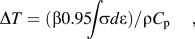
where ∫σdε is the area under the uncorrected stress strain curve, ρ and C p are the density and specific heat of the alloy, respectively. The factor, 0.95, represents part of the total mechanical work that is transformed to heat, with the remaining being used up in microstructural changes.Reference Prasad and Sasidhara34 The value of β, the adiabatic correction factor, is the fraction of the adiabatic heat retained in the workpiece without being lost to the dies, given by,

Typically, β is assumed to be independent of strain and temperature, which is also the assumption made in this work. There have been a few instances that have been reported in literature which contradict this behavior.Reference Charpentier, Store, Earnest and Thomas35, Reference Oh, Semiatin and Jonas36 The value of β in this study varies from 0 at  = 0.001 s−1 to 1.0 at
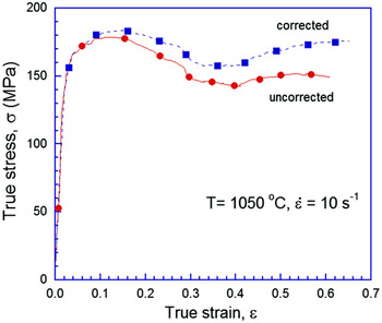
 = 10 s−1, which is in accordance with Ref. Reference Goetz and Semiatin33. Figure 4 is a representative plot which compares the adiabatic corrected (dashed line) and uncorrected (solid line) stress–strain responses at T = 1050 °C and
 = 10 s−1. The calculated (and independently observed by means of the thermocouple) temperature rise was negligible at lower strain rates. Expectedly, the adiabatic contribution was quite significant at higher strain rates, which resulted in a shift of the σ–ε curves in the higher strain rate regime (beyond 1 s−1).
Representative plot showing a comparison of adiabatic corrected and uncorrected stress strain responses. As strain rate increases, the corrected curve moves upward.

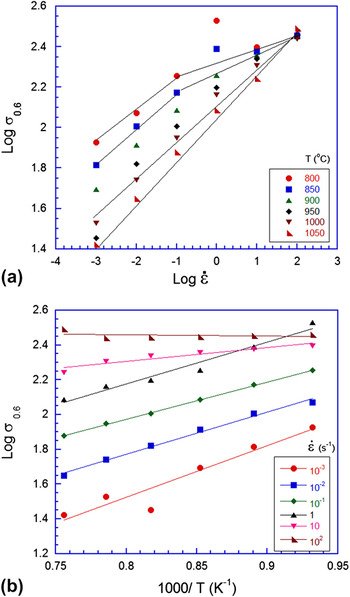
The variation of flow stress (adiabatic corrected) at a true strain of 0.6 with strain rate and temperature are plotted in Figs. 5(a) and 5(b), respectively. A power law

Variation of flow stress at a true strain of 0.6 with (a) strain rate and (b) temperature.

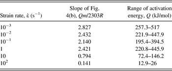
where K is a constant and m is the strain rate sensitivity is used to describe the trends. It can be seen that in Fig. 5(a), the points follow a linear fit (on a log–log graph), with the slope, m varying between 0.1 and 0.21 with the data converging in the lower temperature regime. In fact, a bilinear trend can be observed at lower temperatures (illustrated for lowest temperature), whereas the curve stays linear at high temperatures. The value of m can be utilized to get a range of activation energies from the slopes of flow stress versus (1/T) data at each strain rate. When flow stress at true strain of 0.6 is plotted against 1000/T [as shown in Fig. 5(b)], the slope obtained is Qm/2303R, where R is the universal gas constant (the 2303 results from conversion to logarithm of base 10) and Q is the activation energy. Estimated values of Q are listed in Table II, which suggests that Q reduces at higher  . This is mainly due to significant softening observed in the low T, high strain rate regime at ε = 0.6. Our efforts to compare these values with the literature data did not succeed as there are only a couple of studies, which examined the creep behavior of NiTi alloys in similar temperature regimes.Reference Mukherjee37, Reference Kato, Yamamoto, Hashimoto and Miura38 They, however, have tested the specimens in the low strain rate regimes only.
Activation energies, Q, at different strain rates.

B. Processing maps
The values of m were computed for each sample and at different temperatures from the local values (fit by a cubic spline) of slopes of the logarithmic plots of σ– .Reference Prasad and Sasidhara34, Reference Prasad39 A true strain value of 0.6 was used for the purpose. The efficiency of power dissipation, η, for microstructural changes is obtained asReference Prasad and Sasidhara34, Reference Prasad39
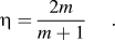
Isoefficiency contour maps in the two-dimensional (2D) space of T and  (η maps) are utilized to identify different deformation mechanisms that exist over different combinations of T and
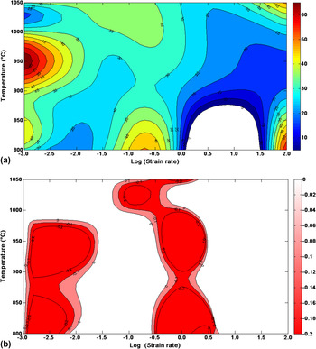
 . A 2D contour efficiency map for the NiTiCu alloy is shown in Fig. 6(a). Several high-efficiency regimes can be noted in the high strain rate corners of the map and also at medium strain rate–low-temperature regime. The maximum value of η in the map occurs at 950 °C and 10−3 s−1. Areas where the calculated efficiency is negative were set to zero (observed in the white regions of the efficiency map). The dynamic recrystallization (DRX) regime, which is important from the workability point of view, typically exhibits the highest values of η over a broad range with widely spaced contours indicating small gradation to the efficiency hill.Reference Prasad and Sasidhara34, Reference Prasad39 The width of the DRX regime obtained from the processing maps will dictate the limits, in terms of T and
 , for the industrial hot working schedule. However, a region with extremely high η value (>90) in the efficiency map can be misleading; it is also usually associated with void formation or it could also be an indication of a superplastic regime as well. Void formation is characterized by a rapid rise in η with the decrease in temperature. Therefore, the information from processing maps alone is insufficient to conclude about deformation mechanisms of a particular material.
Two-dimensional contour maps of (a) efficiency and (b) instability parameter at a true strain of 0.6.

An instability criterion, which is based on the maximum rate of entropy production, given by the following equation,Reference Prasad and Sasidhara34, Reference Prasad39
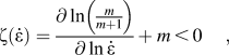
where ζ( ) is a dimensionless parameter that represents the instability in the system is used. Equation (5) is the condition for microstructural stability at a constant value of applied strain expressed in terms of ζ(
 ). Similar to η maps, 2D ζ contour maps can also be generated in the 2D T–
 space for a fixed value of ε. The region of instability is indicated areas in the map which have a negative ζ value. Instability can be inferred due to defects in processing, i.e., formation of cavities, shear band formation, flow localization, breaking of particles, etc.Reference Prasad and Sasidhara34 The η and ζ maps when superposed together can then be utilized to identify the domains that are suitable for hot working/industrial practice. They can be used as a thumb rule to prevent undesirable microstructures by avoiding regions of instability in the maps. The processing map approach has been successfully implemented to accurately predict hot working conditions for a large variety of metals and alloys (see for example, Refs. Reference Prasad and Sasidhara34, Reference Prasad39, Reference Sen, Kottada and Ramamurty40).
The instability map for the NiTiCu alloy is displayed in Fig. 6(b) (lower limit of color coding stopped at −0.2 to just indicate negative regions of the map). The areas in Fig. 6(b) with a positive value (white regions of the map) of the instability parameter indicate favorable regions for deformation. It can be observed that regions of instability exist in two different zones: low  –T range and at intermediate
 . In the lower regime, the value of instability parameter is low (about −0.2), whereas in the other (larger) regime, it spikes all the way up to −5.
C. Microstructures
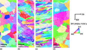
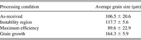
Microstructures obtained using the EBSD for as-received alloy and three different representative deformation conditions are shown in Fig. 7. (We note here that the purpose of conducting EBSD was not to go in detail into the texture evolution during deformation. Rather, the main purpose was to obtain microstructures as conventional “polishing–etching–optical microscopy” route proved to be futile.) The latter three correspond to regions of (a) instability (900 °C and 1 s−1), (b) maximum efficiency (950 °C and 0.001 s−1), and (c) grain growth (1050 °C and 0.001 s−1). These three conditions are referred to as RI, ME, and GG here afterwards, whereas the as-received condition is referred to as AR. From Fig. 7, it is seen that relatively strain-free equiaxed grain structure is present in the AR sample. Some grain refinement takes place in the ME regime, indicating that this combination of temperature and strain rate correspond to that of the DRX regime. GG can be seen in Fig. 7(d), which is taken from the sample that was deformed at the highest temperature and at the slowest strain rate, factors that help GG. It can be seen that there is considerable amount of streaking and “spread” in color in the instability region (IR) sample when compared to patterns of the other samples. This indicates that there is possibly some “remnant strain” in the sample (more on this later.) The average grain sizes for each of these cases have been indicated in Table III. The RI sample did not show any major departure from the initial grain size.
Electron backscatter diffraction patterns of samples in (a) as-received (AR), (b) instability region (IR), (c) maximum efficiency (ME), and (d) grain growth (GG) regions of the processing map. The mentioned regions have been explained in the text.

Average grain sizes of the samples processed in four different regions of the processing map.
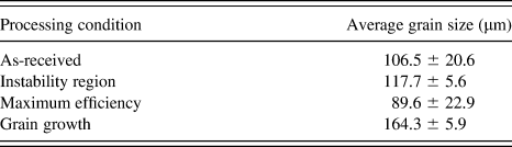
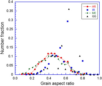
Figure 8(a) shows the distribution of GAR for each case. Here, GAR is obtained by approximating every grain to an ellipse and the ratio of length of minor to major axis for every grain averaged over the scan area is taken as GAR. Both the AR and ME samples show a bell-shaped symmetric distribution with a maximum around 0.45, whereas both RI and GG samples show distributions that are skewed in favor of higher values of GAR.
Distribution of grain aspect ratio for various sample processing conditions.

In EBSD, the quality of the obtained images depends largely on material-related parameters like crystal structure and orientation, composition, surface condition, and sample preparation. When the periodicity of the underlying crystal structure of the grain is disturbed by defects in the range of the interaction volume, the quality of patterns suffer, i.e., they become more diffuse. Thus, the image quality parameters can be used to assess remnant plastic strain and recrystallization kineticsReference Lehockey, Lin, Lepik, Schwartz, Kumar and Adams41, Reference Randle and Engler42 and are related to retained defect content in a region close to the sample surface. There are other practical difficulties that can arise as well. As a result, other metrics such as misorientation density analysis, which uses variations in crystal orientation to elucidate the state of recrystallization in observed microstructure, is advantageous in characterizing residual plastic deformation over traditional image quality measurements.Reference Lehockey, Lin, Lepik, Schwartz, Kumar and Adams41 In this study, a point-to-point misorientation method called kernel average misorientation (KAM) was used to analyze the microstructure obtained in the four cases. In every case, a scan area of approximately 0.3 × 0.9 mm2 close to the center of the specimen (and oriented such that the length of the scan corresponds to the compression axis/z direction of the specimen) was used for analysis of residual plastic strain. Here, local misorientation was characterized using a misorientation kernel approach. For a given point, the average misorientation of that particular point with all its neighbors (immediate neighbors in the perimeter of the kernel in this case) was calculated with the proviso that misorientations exceeding some tolerance value (in this case, it was 5°) are excluded from the averaging calculation. The value of KAM thus obtained is then assigned to the center of the chosen kernel.
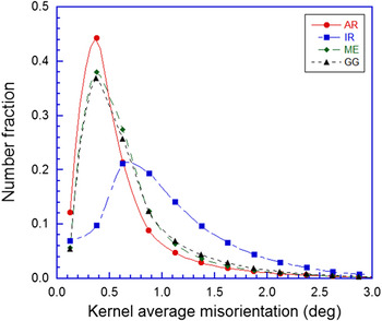
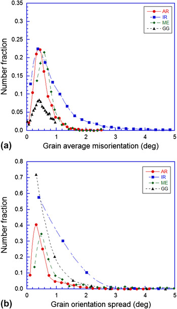
Figure 9 is a plot of the misorientation parameter KAM for all the samples. The sample IR showed a departure from the frequency distribution of other samples in the sense that the KAM distribution is much shallower in the low misorientation domain as compared to the AR sample. On the other hand, the GG and ME samples displayed similar behavior to the AR sample, i.e., a peak was observed close to 0.5°, with around 80% of the points in the scan lying below a KAM value of 0.8°. In contrast, for the IR sample, the corresponding KAM value below which 80% of the points in the scan lie within is approximately 1.3°, which indicates that the sample in the IR region does not recrystallize during deformation and hence carries residual strain when compared to the other cases. A similar behavior can be seen in Figs. 10(a) and 10(b) where other misorientation metrics like grain average misorientation (GAM—the misorientation between every individual pair of points in a grain averaged out over the entire grain) and grain orientation spread (GOS—the average of misorientations of every individual point in a grain when compared to the average orientation of the grain) have been plotted for each of the processing conditions. In each case, the values of misorientation are much larger for the sample which was deformed in the IR, which indicates that the remnant plastic strain in the IR sample is much greater than the other samples in “good” working conditions. This in turn manifests as higher misorientation when the EBSD patterns were utilized for point-to-point analysis within individual grains over a large scan area (KAM/GAM/GOS).
Distribution of kernel average misorientation for various sample processing conditions.

Distribution of (a) grain average misorientation and (b) grain orientation spread for various sample processing conditions.

Even though the ME area may appear to be suitable for metal working, for industrial practice, the proximity of the ME point to the IR could be a potential problem. That said, in industrial conditions, it is much easier to control strain rate than temperature. However, for a truly “safe” window for industrial processing is in the range of 800–850 °C and at 0.1 s−1, appears to be more suitable for industrial practice. The microstructure of the alloy that was obtained after deformation in this condition is nearly identical to that obtained in the ME condition (hence it was not shown here).
IV. SUMMARY
The hot deformation behavior of a Ni42Ti50Cu8 SMA was studied with a view of controlling the microstructure of the finished product during material processing. The processing maps approach was used to generate 2D contour maps of efficiency and instability parameter maps in the range of temperatures between 800 and 1050 °C and at a range of strain rates between 10−3 and 102 s−1. EBSD patterns were analyzed by various misorientation metrics on samples processed in different processing conditions. Using the DRX regime for processing results in grain refinement and strain-free grains. Regions of the instability (having a negative value of instability parameter) indicate higher remnant strains, which are likely to affect the performance of the SMA. A processing window suitable for industrial practice was suggested.
ACKNOWLEDGMENTS
The authors acknowledge financial support by Rolls–Royce Plc and The Boeing Company for this work. The authors are also thankful to S. Sasidhara and K. Rajasimha for their assistance in conducting the compression experiments, K. Shyamprasad for his help in writing the code that is used for the processing maps, and R. Basu for conducting the EBSD scans at the National Facility (OIM and x-ray bulk texture) at IIT-B under the guidance of I. Samajdar. Technical discussions with Y.V.R.K. Prasad, R.S. Kottada, I. Sen, and K. Suresh, which helped this work in many ways, are gratefully acknowledged.