

1 Introduction
The mixing layer emerging from the interaction of two parallel streams characterized by different velocities  $U_{1}$ and
 $U_{2}$ is a classical paradigm case for free-shear turbulent flows. This case has been widely investigated via numerical simulation in time evolution, see e.g. Sandham & Reynolds (Reference Sandham and Reynolds1991), Rogers & Moser (Reference Rogers and Moser1994), Balaras, Piomelli & Wallace (Reference Balaras, Piomelli and Wallace2001) and Delport, Baelmans & Meyers (Reference Delport, Baelmans and Meyers2011), or in space evolution, as in e.g. Yee, Sandham & Djomehri (Reference Yee, Sandham and Djomehri1999), McMullan, Gao & Coats (Reference McMullan, Gao and Coats2007), Wang, Tanahashi & Miyauchi (Reference Wang, Tanahashi and Miyauchi2007), Meldi, Salvetti & Sagaut (Reference Meldi, Salvetti and Sagaut2012), Meldi & Poux (Reference Meldi and Poux2017) and Hug & McMullan (Reference Hug and McMullan2019). The investigations reported in the literature indicate that the emergence and evolution of turbulent features for this flow configuration exhibit high sensitivity to the parametric set-up of the test case. Among these parameters, the shear intensity
 $\unicode[STIX]{x1D6FC}=(U_{1}-U_{2})/(U_{1}+U_{2})$, which measures the intensity of the shear effect versus the average advection, plays a dominant role in the mixing-layer evolution (Rogers & Moser Reference Rogers and Moser1994; Pope Reference Pope2000). However, numerous other features of the inlet flow, which might not be exactly estimated or controllable in practical applications or even experiments, can affect the features of the turbulent mixing region. In particular, one assumption for classical analysis of mixing layers is that
 $U_{1}$ and
 $U_{2}$ are perfectly aligned. Real cases usually involve effects leading to the emergence of a three-dimensional behaviour of the flow, such as variations of the velocity of the streams in the spanwise direction (see e.g. Fiedler et al. Reference Fiedler, Nayeri, Spieweg and Paschereit1998).
Many practical applications, such as those involving three-dimensional flow separations, are characterized by a skew angle between the two streams. Complex test cases of industrial interest include the flow around blades in compressors and turbines, three-dimensional boundary layer separation over wings as well as the flow around vehicles operating with lateral wind gust conditions. When compared with the comprehensive literature references of the classical test case, mixing layers exhibiting skew angles have been addressed much more rarely. Experimental studies can be found in Hackett & Cox (Reference Hackett and Cox1970), Fiedler et al. (Reference Fiedler, Nayeri, Spieweg and Paschereit1998) and Naughton, Cattafesta & Settles (Reference Naughton, Cattafesta and Settles1997). The first two studies consider large skew angles, while the work by Naughton et al. (Reference Naughton, Cattafesta and Settles1997) investigates several values of the normalized swirl parameter for the turbulent round jet case. The values investigated roughly correspond to a skew angle  $\unicode[STIX]{x1D703}\in [\unicode[STIX]{x03C0}/12,\unicode[STIX]{x03C0}/3]$. Stability studies for skewed mixing layers were reported in Lu & Lele (Reference Lu and Lele1993, Reference Lu and Lele1999a,Reference Lu and Leleb). In particular, Lu & Lele (Reference Lu and Lele1993) explored configurations for
 $\unicode[STIX]{x1D703}\in [0,\unicode[STIX]{x03C0}/2]$ and they found that the amplification rate of disturbances grows with the skew angle. This effect becomes more significant as
 $\unicode[STIX]{x1D6FC}$ decreases.
In the present study, we focus on small skew angles and on how parametric variations applied at the inlet affect the evolution of the flow. The motivation for this choice is threefold. Small skew angles can be a consequence of the epistemic uncertainties affecting experiments, and, thus, a description of their effect can be important for the comparison between numerical and experimental results. Also, a non-trivial question is how such perturbations may affect the evolution of the flow. Thus, uncontrolled perturbations in the alignment of the co-flows may be responsible for difficulties in reliable comparison between experimental and numerical results. In particular, effects may emerge due to the interactions of  $\unicode[STIX]{x1D703}$ and
 $\unicode[STIX]{x1D6FC}$ over the evolution of the mixing layer and on the flow features in both the initial transitional region and the turbulent region downstream. Moreover, the impact of skew angles on the turbulence features, as e.g. the components of the Reynolds stress tensor, may give useful indications for the development of turbulence or subgrid-scale models for shear flows in which skew effects are present. As previously said, this kind of flow is relevant to many applications of practical interest. Finally, the last question is how these three-dimensional features, due to a small skew angle, can be exploited to control the flow configuration optimizing some key features, such as the mixing-layer growth rate or the related mixing. In addition, a second objective is the determination of what degree of accuracy in the prescribed value of the skew angle is required to exploit such control techniques. These strategies are envisioned in the framework of parametric variation, which can only be applied at a specific location in space, such as for actuators. In the present study, the parametric variation is applied at the inlet, and the emergence of associated features of the flow is investigated.
To address these aims, a comprehensive sensitivity analysis of the statistical features of spatially evolving mixing layers to three-dimensional effects due to a small skew angle between the streams is performed. The sensitivity analysis includes a second parameter of investigation, the shear intensity parameter  $\unicode[STIX]{x1D6FC}$. This parameter is analysed over an extended range, which includes the values used in previous studies in the literature on classical mixing layers (Mehta Reference Mehta1991; Slessor, Bond & Dimotakis Reference Slessor, Bond and Dimotakis1998; Wang et al. Reference Wang, Tanahashi and Miyauchi2007; McMullan, Gao & Coats Reference McMullan, Gao and Coats2009; Attili & Bisetti Reference Attili and Bisetti2012) and which are relevant to practical application. As previously discussed, this parameter has a remarkable impact on the development of classical mixing layers, in particular in the fully developed turbulence region, downstream from the inlet. In the present study, the focus is on the features of the flow in this region, although the initial transitional region is also analysed. The research work is developed using instantaneous and time-averaged results obtained from a database of 18 direct numerical simulations (DNS). Each simulation is run for prescribed, fixed values for
 $\unicode[STIX]{x1D703}$ and
 $\unicode[STIX]{x1D6FC}$. In addition, a stochastic methodology relying on tools from uncertainty quantification (UQ) is adopted.
Stochastic approaches have been increasingly used in the past few years for uncertainty quantification and sensitivity analysis in numerical simulation of turbulent flows (see e.g. Lucor, Meyers & Sagaut Reference Lucor, Meyers and Sagaut2007; Ko, Lucor & Sagaut Reference Ko, Lucor and Sagaut2008; Meldi et al. Reference Meldi, Salvetti and Sagaut2012; Gorle & Iaccarino Reference Gorle and Iaccarino2013; Edeling et al. Reference Edeling, Cinnella, Dwight and Bijl2014; Margheri et al. Reference Margheri, Meldi, Salvetti and Sagaut2014; Mariotti et al. Reference Mariotti, Salvetti, Omrani and Witteveen2016; Wu, Wang & Xiao Reference Wu, Wang and Xiao2016; Mariotti, Siconolfi & Salvetti Reference Mariotti, Siconolfi and Salvetti2017; Edeling, Iaccarino & Cinnella Reference Edeling, Iaccarino and Cinnella2018; Xiao & Cinnella Reference Xiao and Cinnella2019). In this framework, the two input parameters investigated are considered as random variables with a given probability distribution over the range of investigation prescribed. The uncertainty is then propagated through the computational model to statistically quantify their effect on the results. In order to reduce the computational costs, a surrogate model is used to build a continuous response surface in the parameter space starting from the DNS available in the database. The stochastic tools then provide the complete response surface from the database of DNS performed. This non-intrusive approach is based on the tool known as generalized polynomial chaos (Xiu & Karniadakis Reference Xiu and Karniadakis2002; Lucor & Karniadakis Reference Lucor and Karniadakis2004; Le Maître & Knio Reference Le Maître and Knio2011). This tool relies on the representation of the quantities of interest in the uncertainty space using an orthonormal polynomial basis for the uncertain random parameters.
The paper is organized as follows. In § 2 the numerical solver used to perform the DNS is presented together with the simulation set-up. In § 3 details about the gPC approach and the stochastic investigation strategy are provided. In § 4 a parametric analysis of the flow sensitivity to the considered parameters is carried out by considering time-averaged and instantaneous features of the velocity field. In § 5 a comprehensive stochastic analysis of a number of statistics is performed. Discussion bridging instantaneous structural organization of the flow and stochastic analysis is developed. Finally, in § 6 the concluding remarks are drawn.
2 Numerical methodology and simulation set-up
The DNS are performed by numerical discretization of the Navier–Stokes equations for incompressible flow through the open-source C++ library OpenFOAM (OpenCFD 2004). This is a well-known tool used in recent years in computational fluid dynamics and based on a face-centred finite-volume method. More precisely, the numerical fluxes are here computed using second-order centred schemes, while the time derivative is discretized using an explicit second-order backward scheme. Finally, a PISO (pressure implicit with splitting of operators) algorithm is adopted to solve the system formed by the discretized Navier–Stokes equation and the Poisson equation that implements the solenoidal field incompressibility condition (Issa Reference Issa1986; Ferziger & Peric Reference Ferziger and Peric2001).
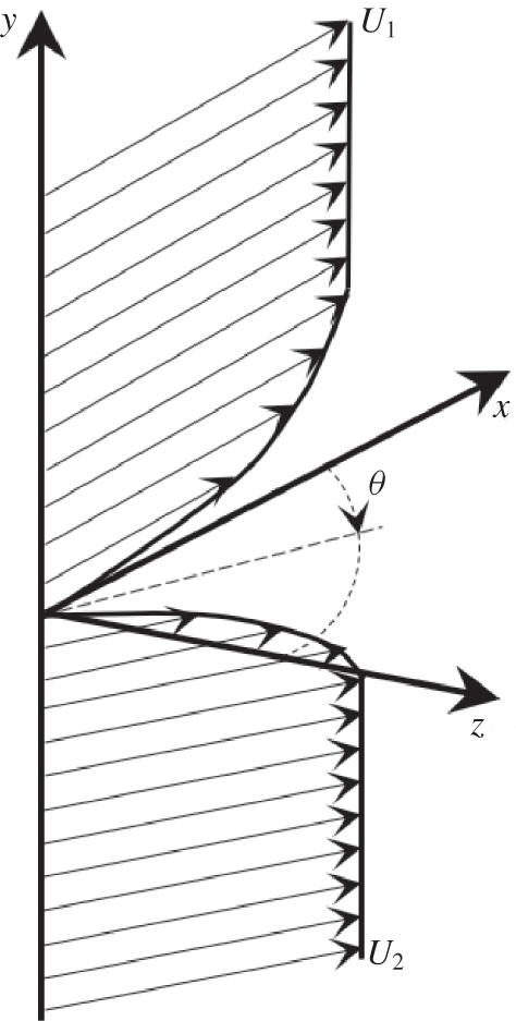
As previously discussed, the turbulent spatially evolving mixing layer is characterized by the interaction of two homogeneous co-flows having different asymptotic velocities,  $\boldsymbol{U}_{1}$ and
 $\boldsymbol{U}_{2}$. In classical analyses, the frame of reference is usually defined so that
 $x$ is the streamwise direction of the two asymptotic streams,
 $y$ is the normal (or cross-wise) direction in which asymptotic velocity gradients are observed and
 $z$ is the spanwise direction. In this work, the lack of perfect alignment between the two asymptotic velocities is measured by the skew angle
 $\unicode[STIX]{x1D703}$, which is constant and measured on the
 $x{-}z$ planes. The frame of reference has been chosen so that the higher asymptotic velocity,
 $U_{1}$, is aligned with the streamwise direction
 $x$ and
 $\boldsymbol{U}_{1}=[U_{1}^{x},U_{1}^{y},U_{1}^{z}]=[U_{1},0,0]$. A sketch is shown in figure 1. Therefore, the lower asymptotic velocity,
 $U_{2}$, can be represented in this frame of reference as
 $\boldsymbol{U}_{2}=[U_{2}^{x},U_{2}^{y},U_{2}^{z}]=[U_{2}\cos \unicode[STIX]{x1D703},0,U_{2}\sin \unicode[STIX]{x1D703}]$. As a consequence, the mean flow velocity and the velocity gradient must be determined using vector norms, which are here reported for the sake of clarity:
 $$\begin{eqnarray}\displaystyle & \Vert \boldsymbol{U}_{j}\Vert =\sqrt{(U_{j}^{x})^{2}+(U_{j}^{y})^{2}+(U_{j}^{z})^{2}}, & \displaystyle\end{eqnarray}$$
 $$\begin{eqnarray}\displaystyle & \Vert \boldsymbol{U}_{1}+\boldsymbol{U}_{2}\Vert =\sqrt{(U_{1}+U_{2}\cos \unicode[STIX]{x1D703})^{2}+(U_{2}\sin \unicode[STIX]{x1D703})^{2}}, & \displaystyle\end{eqnarray}$$
 $$\begin{eqnarray}\displaystyle & \Vert \boldsymbol{U}_{1}-\boldsymbol{U}_{2}\Vert =\sqrt{(U_{1}-U_{2}\cos \unicode[STIX]{x1D703})^{2}+(U_{2}\sin \unicode[STIX]{x1D703})^{2}}. & \displaystyle\end{eqnarray}$$
Sketch of the mixing layer.

For every simulation, the Reynolds number is  $Re_{\unicode[STIX]{x1D6FF}}=\unicode[STIX]{x1D6FF}\Vert \boldsymbol{U}_{1}-\boldsymbol{U}_{2}\Vert /\unicode[STIX]{x1D708}=200$, where
 $\unicode[STIX]{x1D6FF}$ is the value of the vorticity thickness imposed at the inlet and
 $\unicode[STIX]{x1D708}$ is the kinematic viscosity of the flow. These two physical parameters are the same for every simulation, which implies as well that
 $\Vert \boldsymbol{U}_{1}-\boldsymbol{U}_{2}\Vert$ is a constant. The flow is investigated in a physical domain of size
 $[x]\times [y]\times [z]\in [0,24\unicode[STIX]{x1D6EC}]\times [-9\unicode[STIX]{x1D6EC},6\unicode[STIX]{x1D6EC}]\times [-3\unicode[STIX]{x1D6EC},3\unicode[STIX]{x1D6EC}]$. Here
 $\unicode[STIX]{x1D6EC}=c_{inst}\unicode[STIX]{x1D6FF}=15.4\unicode[STIX]{x1D6FF}$ is the characteristic primary instability length for the Reynolds number investigated (McMullan et al. Reference McMullan, Gao and Coats2009; Delport et al. Reference Delport, Baelmans and Meyers2011). The parameters mainly affecting the value of the coefficient
 $c_{inst}$ are the Reynolds number and the perturbations imposed at the inlet. As will be discussed in the following, these parameters are fixed in the present analysis for each simulation. Thus, we can expect that
 $\unicode[STIX]{x1D6EC}$, which is a measure of the characteristic length of organization of the coherent structures, should be weakly affected by the parameters
 $\unicode[STIX]{x1D703}$ and
 $\unicode[STIX]{x1D6FC}$ (if at all). Such a large domain, in particular in the normal direction
 $y$, has been chosen in order to minimize the effect of boundary conditions over the flow evolution.
Furthermore, a traction-free condition is imposed at both normal boundaries, while periodic boundary conditions are used in the spanwise  $z$ direction. At the inlet, a hyperbolic tangent mean velocity profile is specified:
 $$\begin{eqnarray}u^{i}(x=0,y,z)=\frac{U_{1}^{i}+U_{2}^{i}}{2}+\frac{U_{1}^{i}-U_{2}^{i}}{2}\,\text{tanh}\left(\frac{2y}{\unicode[STIX]{x1D6FF}}\right).\end{eqnarray}$$
This steady velocity distribution is perturbed in both space and time to trigger the transition to turbulence. As for the perturbation in space, we adopted three-dimensional perturbations related to the position in the spanwise direction (see Colonius & Lele Reference Colonius and Lele1997) as follows:
 $$\begin{eqnarray}\displaystyle & \displaystyle P_{s}(z)=\mathop{\sum }_{g}2\cos (g\,fz),\quad g=1,2,3,~f=2\unicode[STIX]{x03C0}/\unicode[STIX]{x1D6EC},~z\in [0,6\unicode[STIX]{x1D6EC}], & \displaystyle\end{eqnarray}$$
 $$\begin{eqnarray}\displaystyle & \displaystyle u_{s}^{i}(x=0,y,z)=0.005\frac{\Vert \boldsymbol{U}_{1}+\boldsymbol{U}_{2}\Vert }{2}P_{s}(z)\exp (-0.5\sqrt{y/\unicode[STIX]{x1D6FF}}), & \displaystyle\end{eqnarray}$$
where  $u_{s}^{i}$ is the spatial perturbation in the direction
 $i$, applied to the mean velocity profile in (2.4). The perturbation is the same in each spatial direction
 $i$.
Finally, the resulting velocity profile has been perturbed at each time step by a white noise signal of maximum magnitude 2 % at the centreline. The resulting time perturbation  $u_{t}^{i}$ is the following:
 $$\begin{eqnarray}u_{t}^{i}(x=0,y,z)=0.02(2(\text{rand}(t)-0.5))(u^{i}+u_{s}^{i})\exp (-0.5\sqrt{y/\unicode[STIX]{x1D6FF}_{0}}),\end{eqnarray}$$
where  $\text{rand}(t)$ is a random variable with uniform probability density function (p.d.f.) included in the range
 $[0,1]$. This time perturbation is filtered out outside
 $y=[-\unicode[STIX]{x1D6EC},\unicode[STIX]{x1D6EC}]$. Thus, the total velocity imposed at the inlet for each velocity component is
 $u_{inlet}^{i}=u^{i}+u_{s}^{i}+u_{t}^{i}$.
Analyses using the stability theory for the mixing layer have traditionally investigated the sensitivity of the evolution of the flow to variations in the parametric description of the inlet. In particular, it is well known that the shape of the perturbation has a significant impact on the initial growth of the mixing layer (Ho & Huerre Reference Ho and Huerre1984; Lu & Lele Reference Lu and Lele1993; Ko et al. Reference Ko, Lucor and Sagaut2008). Thus, this could be an additional aspect worthy of investigation in combination with  $\unicode[STIX]{x1D703}$ and
 $\unicode[STIX]{x1D6FC}$. However, this would significantly increase the number of parameters to be investigated. Keeping in mind that each DNS requires large computational costs, including these additional parameters is presently unaffordable. We therefore use the previously specified perturbation shape for every simulation. Although the sensitivity to
 $\unicode[STIX]{x1D703}$ and
 $\unicode[STIX]{x1D6FC}$ observed in the initial mixing-layer evolution may be specific to the adopted perturbation, the flow behaviour in the fully turbulent region downstream may reasonably be assumed to be almost independent of it. Finally, an advective velocity condition is used at the outlet, in order to reduce as much as possible reflective waves in the physical domain (Salvetti, Orlandi & Verzicco Reference Salvetti, Orlandi and Verzicco1996; Meldi & Poux Reference Meldi and Poux2017).
Each simulation of the database is run for the same Reynolds number  $Re_{\unicode[STIX]{x1D6FF}}=100$. Also, as previously mentioned, the vorticity thickness
 $\unicode[STIX]{x1D6FF}$ imposed at the inlet is the same for every simulation of the database. This choice for normalization, which is less common than using the asymptotic high-speed velocity, has been adopted in order to use the same mesh for every calculation. This choice precludes uncontrolled numerical effects due to differences in the discretization of the domain. The kinematic viscosity
 $\unicode[STIX]{x1D708}$ is also the same for each simulation and, in particular, the values for the two quantities
 $\unicode[STIX]{x1D6FF}$ and
 $\unicode[STIX]{x1D708}$ are set so that
 $\unicode[STIX]{x1D6FF}/\unicode[STIX]{x1D708}=20~\text{s}~\text{m}^{-1}$. This implies that
 $\Vert \boldsymbol{U}_{1}-\boldsymbol{U}_{2}\Vert =10~\text{m}~\text{s}^{-1}$ is also a constant. The values of the asymptotic velocities
 $U_{1}^{x}$,
 $U_{2}^{x}$ and
 $U_{2}^{z}$ to be imposed at the inlet are then determined, once the values of
 $\unicode[STIX]{x1D703}$ and
 $\unicode[STIX]{x1D6FC}$ are fixed for each simulation. More precisely, the velocity components are obtained resolving this system of three equations, where
 $\unicode[STIX]{x1D703}$,
 $\unicode[STIX]{x1D6FC}$ and
 $\Vert \boldsymbol{U}_{1}-\boldsymbol{U}_{2}\Vert$ are known and
 $U_{1}^{x}$,
 $U_{2}^{x}$ and
 $U_{2}^{z}$ are the unknown variables:
 $$\begin{eqnarray}\displaystyle & \displaystyle \unicode[STIX]{x1D6FC}=\frac{\Vert \boldsymbol{U}_{1}-\boldsymbol{U}_{2}\Vert }{\Vert \boldsymbol{U}_{1}+\boldsymbol{U}_{2}\Vert }, & \displaystyle\end{eqnarray}$$
 $$\begin{eqnarray}\displaystyle & \displaystyle \unicode[STIX]{x1D703}=\text{acos}\left(\frac{U_{2}^{z}}{\Vert \boldsymbol{U}_{2}\Vert }\right), & \displaystyle\end{eqnarray}$$
 $$\begin{eqnarray}\displaystyle & \displaystyle \Vert \boldsymbol{U}_{1}-\boldsymbol{U}_{2}\Vert =\frac{\unicode[STIX]{x1D708}Re_{\unicode[STIX]{x1D6FF}}}{\unicode[STIX]{x1D6FF}}=10~\text{m}~\text{s}^{-1}. & \displaystyle\end{eqnarray}$$
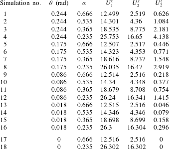
The computed values for the parameters are reported in table 1 for reference.
Database of DNS simulations used in the present analysis. Results from simulations 1–16 are used to reconstruct the response surfaces of the stochastic quantities analysed, by the use of a non-intrusive gPC approach. Simulations 17 and 18 are DNS simulations of the classical mixing-layer configuration.

The structured grid for the simulations is made by hexahedral elements. Extensive discussion about the mesh resolution and validation of the DNS results is reported in appendix A. A constant time step has been fixed choosing the value  $\unicode[STIX]{x0394}t=0.01t_{A}=0.01\times 2\unicode[STIX]{x1D6EC}/(U_{1}+U_{2})$. Here
 $t_{A}$ is the average advection characteristic time. This choice has been performed to ensure that the condition
 $CFL<0.35$ is respected at every time step (
 $CFL$ is the Courant–Friedrichs–Lewy number). Numerical simulations are initialized in the whole physical domain using an unperturbed hyperbolic tangent profile for the velocity equal to the value of
 $u^{i}$ imposed at the inlet, without time or space perturbations. The total simulation time is equal to 250 characteristic times
 $t_{A}$ (equivalent to 25 000 time steps) and statistical quantities are computed starting from
 $t=50t_{A}$ over a time of
 $200t_{A}$.
3 Stochastic sensitivity analysis: methodology and set-up
The generalized polynomial chaos (gPC) method is herein briefly introduced. More detailed discussion can be found in the comprehensive works by Ghanem & Spanos (Reference Ghanem and Spanos1991), Xiu & Karniadakis (Reference Xiu and Karniadakis2002) and Le Maître & Knio (Reference Le Maître and Knio2011).
The sensitivity of physical quantities of the flow to the parameters  $\unicode[STIX]{x1D703}$ and
 $\unicode[STIX]{x1D6FC}$ is cast into a probabilistic framework. Let one consider a random process
 $R$ which is a function of an
 $M$-dimensional random vector
 $\unicode[STIX]{x1D743}=[\unicode[STIX]{x1D709}_{1},\unicode[STIX]{x1D709}_{2},\ldots ,\unicode[STIX]{x1D709}_{M}]$ contained in the parameter space
 $\unicode[STIX]{x1D6FA}\subset \mathbb{R}^{M}$. The non-intrusive gPC approach is a spectral method used to perform a projection of
 $R$ over a known orthogonal polynomial base
 $\unicode[STIX]{x1D6F9}$. The gPC representation can be written using a term-based notation as follows:
 $$\begin{eqnarray}R=\mathop{\sum }_{j=0}^{+\infty }\unicode[STIX]{x1D6FD}_{j}\unicode[STIX]{x1D6F9}_{j}(\unicode[STIX]{x1D743}),\end{eqnarray}$$
where  $\unicode[STIX]{x1D6F9}_{j}(\unicode[STIX]{x1D743})$ is the gPC multivariate polynomial of generic index
 $j$ (which involves products of the one-dimensional polynomials) and
 $\unicode[STIX]{x1D6FD}_{j}$ is the related Galerkin projection coefficient. In practice, the polynomial expansion is truncated to a finite limit,
 $T$:
 $$\begin{eqnarray}R=\mathop{\sum }_{j=0}^{T}\unicode[STIX]{x1D6FD}_{j}\unicode[STIX]{x1D6F9}_{j}(\unicode[STIX]{x1D743}),\end{eqnarray}$$
where  $T$ is a function of the number of considered parameters
 $M$ and of the maximum degree
 $P$ of the retained polynomials. The integrals involved in the computation of the gPC expansion coefficients
 $\unicode[STIX]{x1D6FD}_{j}$ can be computed numerically. A key issue is the choice of the polynomial family used in the gPC expansion. A suitable polynomial family, i.e. able to give an accurate response surface in the parameter space using a few terms in the gPC expansion, depends on the shape of the p.d.f. of the uncertain parameters.
In the framework of the present work, the determination of a suitable p.d.f. for  $\unicode[STIX]{x1D703}$ and
 $\unicode[STIX]{x1D6FC}$ is challenging. In fact, this description is intimately connected with the physical mechanism generating the mixing layer. Thus, p.d.f.s for
 $\unicode[STIX]{x1D6FC}$ would exhibit important differences for practical applications or changing operative conditions. On the other hand, since
 $\unicode[STIX]{x1D703}$ is thought herein to represent an uncontrolled misalignment in experiments or an unknown perturbation of flow control, for this quantity there is no a priori knowledge of the p.d.f. For these reasons, it is here chosen to employ the most simple and general p.d.f. to describe the distribution of the parameters under investigation. More precisely, the p.d.f.s have been considered herein as uniform. Owing to the choice to use uniform p.d.f.s for both parameters, the Legendre polynomial family is employed for the spectral projection in (3.2). This is a well-suited choice since the inner product weighting function is directly proportional to the set p.d.f.
As previously introduced, the skew angle  $\unicode[STIX]{x1D703}$ and the shear parameter
 $\unicode[STIX]{x1D6FC}$ are considered as random uncertain parameters. The uniform p.d.f. describing them is defined over the following ranges.
(i)
 $\unicode[STIX]{x1D703}\in [0,\unicode[STIX]{x03C0}/12]$ rad: As discussed in the introduction, this choice has been performed in order to investigate the effect of a rather small angle between the two streams, which may be interpreted as a controlled or uncontrolled perturbation of the classical mixing-layer configuration.
(ii)
$\unicode[STIX]{x1D6FC}\in [0.2,0.7]$: The size of the range of investigation has been determined after a comprehensive review of the configurations reported in the literature. Experimental analyses are usually performed for low $\unicode[STIX]{x1D6FC}$ values, which correspond to velocity ratios close to unity. For example, Mehta (Reference Mehta1991) performed investigations in the range $\unicode[STIX]{x1D6FC}\in [0.05,0.33]$, Abdul Azim & Sadrul Islam (Reference Abdul Azim and Sadrul Islam2003) in the range $\unicode[STIX]{x1D6FC}\in [0.05,0.18]$ and Slessor et al. (Reference Slessor, Bond and Dimotakis1998) for $\unicode[STIX]{x1D6FC}=0.43$. Conversely, values investigated in numerical simulation are noticeably higher, in order to avoid issues in triggering three-dimensional instabilities observed for similar velocities of the co-flows. Wang et al. (Reference Wang, Tanahashi and Miyauchi2007) and McMullan et al. (Reference McMullan, Gao and Coats2009) employ a value of $\unicode[STIX]{x1D6FC}=0.33$, Attili & Bisetti (Reference Attili and Bisetti2012) chose $\unicode[STIX]{x1D6FC}=0.5$, Yang et al. (Reference Yang, Zhang, Chan and Lin2004) $\unicode[STIX]{x1D6FC}=0.53$ and Hug & McMullan (Reference Hug and McMullan2019) investigated configurations in the range $\unicode[STIX]{x1D6FC}\in [0.33,0.66]$. The present range of investigation includes values used in numerical applications as well as a large part of the configurations studied via experiments.


One could argue that the range of investigation for the parameter  $\unicode[STIX]{x1D6FC}$ is much larger than for the parameter
 $\unicode[STIX]{x1D703}$. This is consistent with the motivation of the present investigation, in which the effect of perturbation in the alignment of two co-flows is studied over a range of operative configurations. At the same time, one can expect that the parameter
 $\unicode[STIX]{x1D6FC}$ will be responsible for larger variations of the physical quantities investigated.
In the present work,  $P=3$ for both the random variables investigated (i.e. a third-order expansion is employed). The analysis of the projection coefficients
 $\unicode[STIX]{x1D6FD}_{j}$ reveals that the contribution of third-order polynomials is very small, as shown in appendix A via the comparison of the results obtained using
 $P=2$ and
 $P=3$. This implies that convergence of the reconstruction of the response surface is well achieved for
 $P=3$, assessing the choice performed in the analysis. The non-intrusive strategy relies on the usage of data from a database of DNS simulations. Each run is performed for fixed values of
 $\unicode[STIX]{x1D703}$ and
 $\unicode[STIX]{x1D6FC}$. A Gaussian quadrature formula is employed here, defining
 $m_{i}=P+1$ quadrature points per parameter. Owing to this choice, input information is needed in four quadrature points for each parameter. This sums up to a total of
 $4^{2}=16$ discrete points in the uncertainty space. For each of these points, a DNS with fixed values for
 $\unicode[STIX]{x1D703}$ and
 $\unicode[STIX]{x1D6FC}$ has been performed. Results have then been reconstructed on the continuous two-dimensional uncertainty space via gPC. In addition, two classical (
 $\unicode[STIX]{x1D703}=0$) numerical simulations have been performed for comparison. The value chosen for
 $\unicode[STIX]{x1D6FC}$ corresponds to the higher/lower value resulting from the Gaussian quadrature, respectively. These values are used to determine the features of the velocity field as reported in (2.8), (2.9) and (2.10).
4 Mixing-layer evolution and features for varying $\unicode[STIX]{x1D703}$ and $\unicode[STIX]{x1D6FC}$


A qualitative analysis of the main instantaneous and time-averaged flow features as obtained in DNS simulations for varying  $\unicode[STIX]{x1D6FC}$ and
 $\unicode[STIX]{x1D703}$ is now developed. Here the reader should be reminded that the variation of the parameters is imposed at the inlet. Thus, the uncertainty in the parametric description affects the whole structural organization of the flow moving downstream. The first physical quantity investigated is the momentum thickness
 $\unicode[STIX]{x1D6E9}$, which is by definition
 $$\begin{eqnarray}\unicode[STIX]{x1D6E9}(x)=\frac{1}{6\unicode[STIX]{x1D6EC}}\frac{1}{(\Vert \boldsymbol{U}_{1}-\boldsymbol{U}_{2}\Vert )^{2}}\int _{-3\unicode[STIX]{x1D6EC}}^{3\unicode[STIX]{x1D6EC}}\int _{-9\unicode[STIX]{x1D6EC}}^{6\unicode[STIX]{x1D6EC}}(\widehat{U_{1}^{x}}(x)-\overline{u_{x}}(x,y,z))\,(\overline{u_{x}}(x,y,z)-\widehat{U_{2}^{x}}(x))\,\text{d}y\,\text{d}z.\end{eqnarray}$$
The quantities indicated with a  $\,\widehat{\;}\,$ denote the value of the velocity outside the mixing layer; the second mesh element far from the boundary, the first that is not directly affected by the boundary traction-free condition, has been used. As is well known, the momentum thickness provides a measure of the growth rate of the mixing layer.
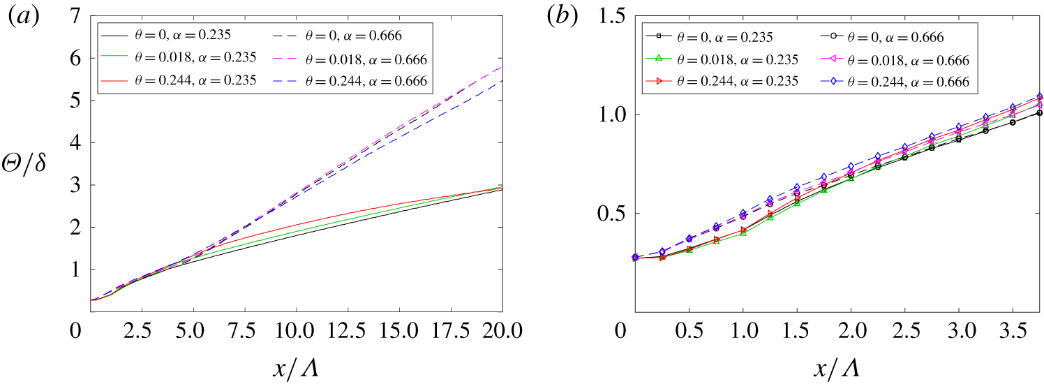
In figure 2 results are shown for the simulations 1, 4, 13, 16, 17 and 18 of the database, i.e. the two classical DNS and the four simulations carried out for the extreme values of  $\unicode[STIX]{x1D6FC}$ and
 $\unicode[STIX]{x1D703}$ in the database. The results in the whole physical domain reported in figure 2(a) indicate that
 $\unicode[STIX]{x1D6FC}$ is the main parameter driving the evolution of
 $\unicode[STIX]{x1D6E9}$. As expected, low-
 $\unicode[STIX]{x1D6FC}$ simulations exhibit a slower increase of
 $\unicode[STIX]{x1D6E9}$. However, for both
 $\unicode[STIX]{x1D6FC}=0.235$ and
 $\unicode[STIX]{x1D6FC}=0.666$ the results from the simulation for
 $\unicode[STIX]{x1D6E9}=0.244$ exhibit remarkable differences when compared with the corresponding classical mixing-layer evolution. The differences are larger for
 $\unicode[STIX]{x1D6FC}=0.235$ and for
 $x/\unicode[STIX]{x1D6EC}>7.5$. On the other hand, the evolution of
 $\unicode[STIX]{x1D6E9}$ in the inlet region for
 $x/\unicode[STIX]{x1D6EC}<4$ is mostly independent of the parameters of investigation, as shown in figure 2(b). This confirms that the initial development of the mixing layer
 $\unicode[STIX]{x1D6E9}$ is governed by the perturbations prescribed at the inlet, which are the same for each simulation. In addition,
 $\unicode[STIX]{x1D703}$ and
 $\unicode[STIX]{x1D6FC}$ have a secondary effect on the mixing-layer growth in this region.
Evolution of the momentum thickness  $\unicode[STIX]{x1D6E9}$ normalized over the initial vorticity thickness
 $\unicode[STIX]{x1D6FF}$. Results are reported for six simulations of the DNS database for (a)
 $x/\unicode[STIX]{x1D6EC}\leqslant 20$ and (b) a zoom for
 $x/\unicode[STIX]{x1D6EC}\leqslant 3.75$.

The analysis of the near-inlet dynamics is now extended to the statistical behaviour of the velocity fluctuations. The integral normalized cross-wise component of the velocity fluctuation energy is defined as
 $$\begin{eqnarray}V=\frac{1}{\Vert \boldsymbol{U}_{1}-\boldsymbol{U}_{2}\Vert ^{2}\unicode[STIX]{x1D6E9}}\iint _{yz}\overline{u_{y}^{\prime }u_{y}^{\prime }}\,\text{d}y\,\text{d}z,\end{eqnarray}$$
where  $u^{\prime }$ represents the fluctuating field and the overbar is the time average. For fully turbulent flows,
 $\overline{u_{y}^{\prime }u_{y}^{\prime }}$ is the cross-wise component of the Reynolds stress tensor.
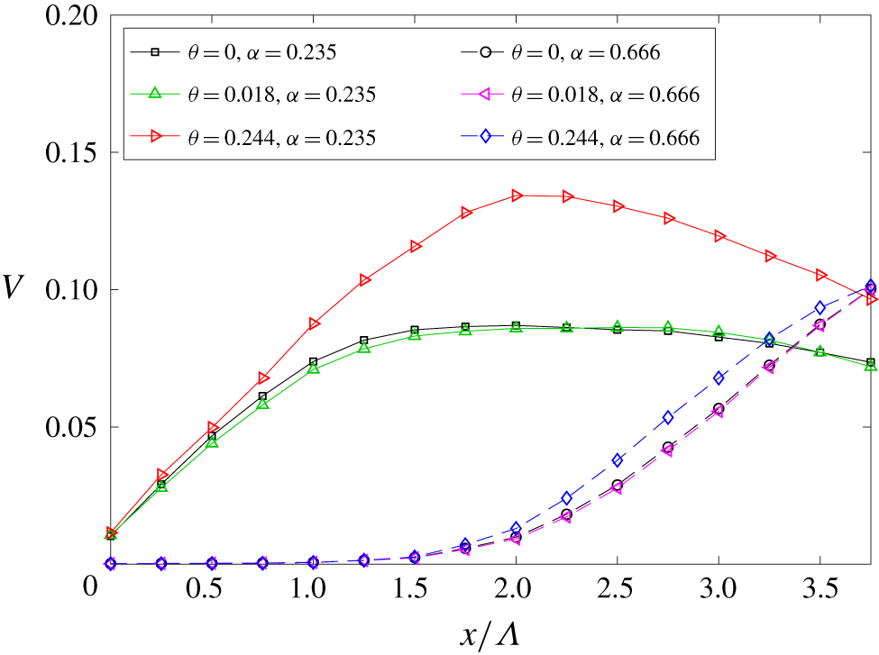
The evolution of  $V$ for
 $x/\unicode[STIX]{x1D6EC}<4$ is reported in figure 3. The behaviour of
 $V$ is governed by the parameter
 $\unicode[STIX]{x1D6FC}$. The simulations for
 $\unicode[STIX]{x1D6FC}=0.235$ exhibit a faster increase of the velocity fluctuating energy when compared with the other DNS investigated. This seems to be related to the perturbations imposed at the inlet, whose energy is proportional to the magnitude of the flow
 $\Vert \boldsymbol{U}_{1}+\boldsymbol{U}_{2}\Vert$ and, thus, inversely proportional to
 $\unicode[STIX]{x1D6FC}$ (as
 $\Vert \boldsymbol{U}_{1}-\boldsymbol{U}_{2}\Vert$ is constant). More interestingly, important differences are again observed for the simulations for
 $\unicode[STIX]{x1D703}=0.244$. For these simulations, the total cross-wise velocity fluctuation energy is significantly increased, in particular for
 $\unicode[STIX]{x1D6FC}=0.235$.
Evolution in space of the integral normalized cross-wise component of the velocity fluctuation energy  $V$ for
 $x/\unicode[STIX]{x1D6EC}\leqslant 3.5$.

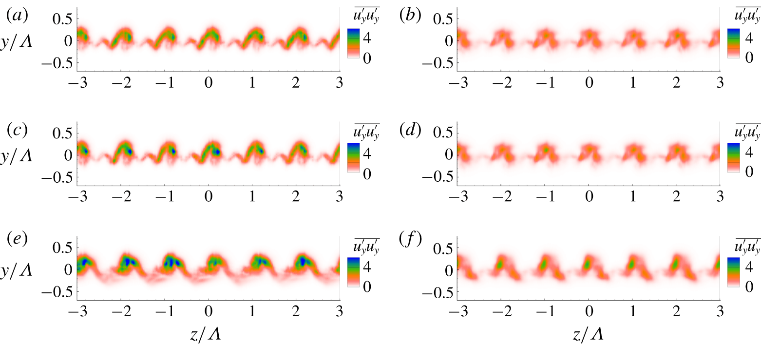
This aspect is further investigated via the analysis of  $\overline{u_{y}^{\prime }u_{y}^{\prime }}$, which is now sampled over two-dimensional
 $y{-}z$ planes for
 $x/\unicode[STIX]{x1D6EC}=3$. This streamwise station has been chosen because
 $V$ is here close to its peak for low-
 $\unicode[STIX]{x1D6FC}$ configurations and it is ramping up for high-
 $\unicode[STIX]{x1D6FC}$ simulations. The isocontours are shown in figure 4. Results from the three simulations for
 $\unicode[STIX]{x1D6FC}=0.666$ are reported in the right column while those for
 $\unicode[STIX]{x1D6FC}=0.254$ are shown in the left column. One can see that the spatial organization of
 $\overline{u_{y}^{\prime }u_{y}^{\prime }}$ is mainly the same for fixed
 $\unicode[STIX]{x1D6FC}$ and it once again reflects the signature of the shape of the inlet spanwise perturbation. The principal difference is the higher magnitude that is exhibited by the case for
 $\unicode[STIX]{x1D703}=0.244$ in figure 4(e,f). Results for
 $\unicode[STIX]{x1D6FC}=0.235$ in the left column of figure 4 exhibit a more complex behaviour. It is thus confirmed that the larger the skew angle, the faster the amplification of the inlet disturbances, and that this effect is more important for low
 $\unicode[STIX]{x1D6FC}$ values. For the particular perturbation considered in the present work, this is consistent with the findings of Lu & Lele (Reference Lu and Lele1993).
Velocity fluctuation energy  $\overline{u_{y}^{\prime }u_{y}^{\prime }}$ sampled at the streamwise station
 $x/\unicode[STIX]{x1D6EC}=3$: (a)
 $\unicode[STIX]{x1D703}=0$ and
 $\unicode[STIX]{x1D6FC}=0.235$, (b)
 $\unicode[STIX]{x1D703}=0$ and
 $\unicode[STIX]{x1D6FC}=0.666$, (c)
 $\unicode[STIX]{x1D703}=0.018$ and
 $\unicode[STIX]{x1D6FC}=0.235$, (d)
 $\unicode[STIX]{x1D703}=0.018$ and
 $\unicode[STIX]{x1D6FC}=0.666$, (e)
 $\unicode[STIX]{x1D703}=0.244$ and
 $\unicode[STIX]{x1D6FC}=0.235$, and (f)
 $\unicode[STIX]{x1D703}=0.244$ and
 $\unicode[STIX]{x1D6FC}=0.666$.

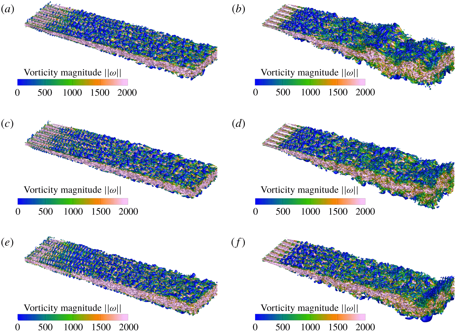
Isosurfaces of the vortex indicator  $\unicode[STIX]{x1D706}_{2}$ coloured by vorticity magnitude: (a)
 $\unicode[STIX]{x1D703}=0$ and
 $\unicode[STIX]{x1D6FC}=0.235$, (b)
 $\unicode[STIX]{x1D703}=0$ and
 $\unicode[STIX]{x1D6FC}=0.666$, (c)
 $\unicode[STIX]{x1D703}=0.018$ and
 $\unicode[STIX]{x1D6FC}=0.235$, (d)
 $\unicode[STIX]{x1D703}=0.018$ and
 $\unicode[STIX]{x1D6FC}=0.666$, (e)
 $\unicode[STIX]{x1D703}=0.244$ and
 $\unicode[STIX]{x1D6FC}=0.235$, and (f)
 $\unicode[STIX]{x1D703}=0.244$ and
 $\unicode[STIX]{x1D6FC}=0.666$.

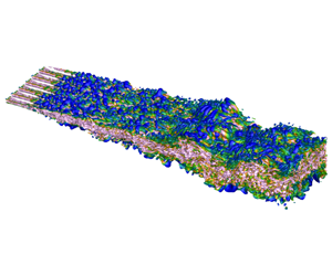
The mixing is now investigated via the analysis of instantaneous vorticity and velocity fields. Figure 5 shows the instantaneous isosurfaces of the vortex indicator  $\unicode[STIX]{x1D706}_{2}$ (Jeong & Hussain Reference Jeong and Hussain1995), coloured by the intensity of vorticity. Figure 5(a,b) reports the results obtained for the classical mixing-layer configuration (
 $\unicode[STIX]{x1D703}=0$) and for the extreme values of
 $\unicode[STIX]{x1D6FC}$. The comparison of the two panels highlights that, for larger values of
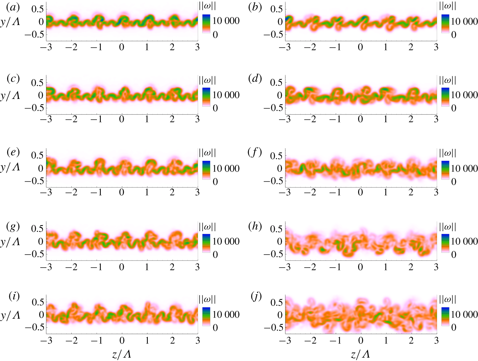
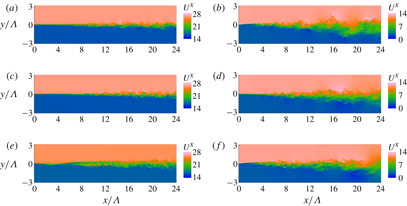
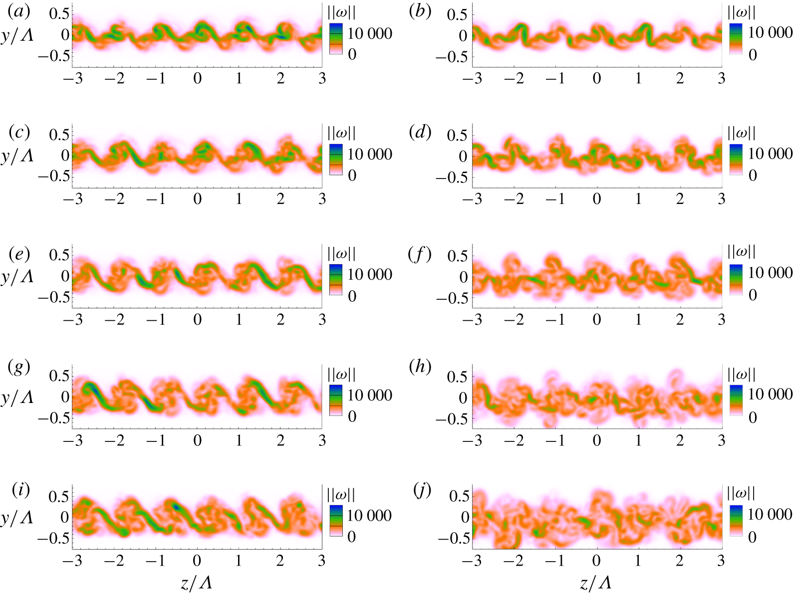
 $\unicode[STIX]{x1D6FC}$, the streamwise coherent structures originated by the inlet spanwise perturbations tend to lose organization more rapidly. This phenomenon comes along with the emergence of progressively smaller three-dimensional structures moving downstream and with a faster growth of the mixing layer, in agreement with the previous analysis of the behaviour of the momentum thickness. These conclusions are reinforced via observation of figures 6 and 7. Vorticity magnitude isocontours are reported in figure 6. The isocontours are shown for
 $y{-}z$ planes for several values of
 $x/\unicode[STIX]{x1D6EC}$. A faster growth of the mixing region for larger
 $\unicode[STIX]{x1D6FC}$ values is clearly visible. Similar conclusions can be drawn analysing the instantaneous streamwise velocity fields (
 $x{-}y$ plane for
 $z=0$) in figure 7(a,b).
Vorticity magnitude for (a,c,e,g,i)  $\unicode[STIX]{x1D703}=0$ and
 $\unicode[STIX]{x1D6FC}=0.235$ and (b,d,f,h,j)
 $\unicode[STIX]{x1D703}=0$ and
 $\unicode[STIX]{x1D6FC}=0.666$ on the planes (a,b)
 $x/\unicode[STIX]{x1D6EC}=3$, (c,d)
 $x/\unicode[STIX]{x1D6EC}=4$, (e,f)
 $x/\unicode[STIX]{x1D6EC}=5$, (g,h)
 $x/\unicode[STIX]{x1D6EC}=6$ and (i,j)
 $x/\unicode[STIX]{x1D6EC}=7$.

Free-stream velocity on the plane  $z/\unicode[STIX]{x1D6EC}=0$: (a)
 $\unicode[STIX]{x1D703}=0$ and
 $\unicode[STIX]{x1D6FC}=0.235$, (b)
 $\unicode[STIX]{x1D703}=0$ and
 $\unicode[STIX]{x1D6FC}=0.666$, (c)
 $\unicode[STIX]{x1D703}=0.018$ and
 $\unicode[STIX]{x1D6FC}=0.235$, (d)
 $\unicode[STIX]{x1D703}=0.018$ and
 $\unicode[STIX]{x1D6FC}=0.666$, (e)
 $\unicode[STIX]{x1D703}=0.244$ and
 $\unicode[STIX]{x1D6FC}=0.235$, and (f)
 $\unicode[STIX]{x1D703}=0.244$ and
 $\unicode[STIX]{x1D6FC}=0.666$.

Vorticity magnitude for (a,c,e,g,i)  $\unicode[STIX]{x1D703}=0.244$ and
 $\unicode[STIX]{x1D6FC}=0.235$ and (b,d,f,h,j)
 $\unicode[STIX]{x1D703}=0.244$ and
 $\unicode[STIX]{x1D6FC}=0.666$ on the planes (a,b)
 $x/\unicode[STIX]{x1D6EC}=3$, (c,d)
 $x/\unicode[STIX]{x1D6EC}=4$, (e,f)
 $x/\unicode[STIX]{x1D6EC}=5$, (g,h)
 $x/\unicode[STIX]{x1D6EC}=6$ and (i,j)
 $x/\unicode[STIX]{x1D6EC}=7$.

Figures 5 and 7 confirm the previous observations on the momentum thickness, i.e. that the presence of a skew angle enhances the mixing-layer growth, in particular for low values of  $\unicode[STIX]{x1D6FC}$. However, in this case the increased mixing-layer growth is not associated with a loss of coherence of the inlet vortical structures, as it conversely happens when increasing
 $\unicode[STIX]{x1D6FC}$, but rather to a faster growth of these structures themselves (see figure 8 showing the same quantities as in figure 6 but for
 $\unicode[STIX]{x1D703}=0.244$). This is consistent with the previous analysis of the normal contribution to the fluctuating velocity energy.
In conclusion, the analysis of the DNS of the database indicates that, as expected, variations of the parameter  $\unicode[STIX]{x1D6FC}\in [0.2,0.7]$ have a primary effect on the growth of the mixing region. This primary effect is associated with bulk shear effects, which are responsible for Kelvin–Helmholtz instabilities and transition to turbulence. However, a secondary effect associated with
 $\unicode[STIX]{x1D703}$ is observed. Higher values for the skew angle magnify the growth of inlet structures, which results in a faster increase of the mixing region. This effect is progressively less visible for higher
 $\unicode[STIX]{x1D6FC}$ values, due to the more rapid transition to turbulence, which then dominates the mixing-layer growth. These results are in agreement with the experimental findings by Naughton et al. (Reference Naughton, Cattafesta and Settles1997). The analysis of the turbulent round jet indicated that the initial evolution of the mixing layers, which was performed for low values of
 $\unicode[STIX]{x1D6FC}\in [0.21,0.4]$, does not show any apparent difference between the swirling mixing layer and the classical non-swirling case. However, moving downstream, both the spatial extent and amplitude of the largest turbulent fluctuations were found to be increased. So, the entrainment associated with an additional source of turbulence production is responsible for a larger mixing layer growth rate.
5 Stochastic analysis of time-averaged flow quantities
The stochastic analysis of some relevant statistical quantities of the flow is used herein to quantify the effects associated with the variability of  $\unicode[STIX]{x1D6FC}$ and
 $\unicode[STIX]{x1D703}$, whose effects were qualitatively described in § 4. The analysis here is performed relying on the use of the gPC to reconstruct multiple response surfaces, considering a uniform p.d.f. for the input parameters
 $\unicode[STIX]{x1D703}$ and
 $\unicode[STIX]{x1D6FC}$. Despite the level of approximation associated with this choice, these results are complementary to the findings obtained in § 4. In particular, they are useful to provide a quantification of the expected variance of the physical quantities over the parametric space investigated, as well as to highlight effects due to interactions of
 $\unicode[STIX]{x1D703}$ and
 $\unicode[STIX]{x1D6FC}$. One should keep in mind that these statistical measures describe the history of the flow when the perturbation is applied upstream at the inlet. Thus, while these measures describe the effects of the uncertainty over the evolution of the flow, they should not be considered as a statistical feature for a localized perturbation.
To this aim, the physical quantities calculated via DNS (such as the time-averaged velocity field) have been sampled on 161 planes normal to the streamwise section  $x$ in the range
 $x\in [4\unicode[STIX]{x1D6EC},20\unicode[STIX]{x1D6EC}]$. The distance between planes is constant and it is equal to
 $0.1\unicode[STIX]{x1D6EC}$. Here we excluded the region
 $x/\unicode[STIX]{x1D6EC}<4$ in order to focus the analysis on the region exhibiting turbulent features.
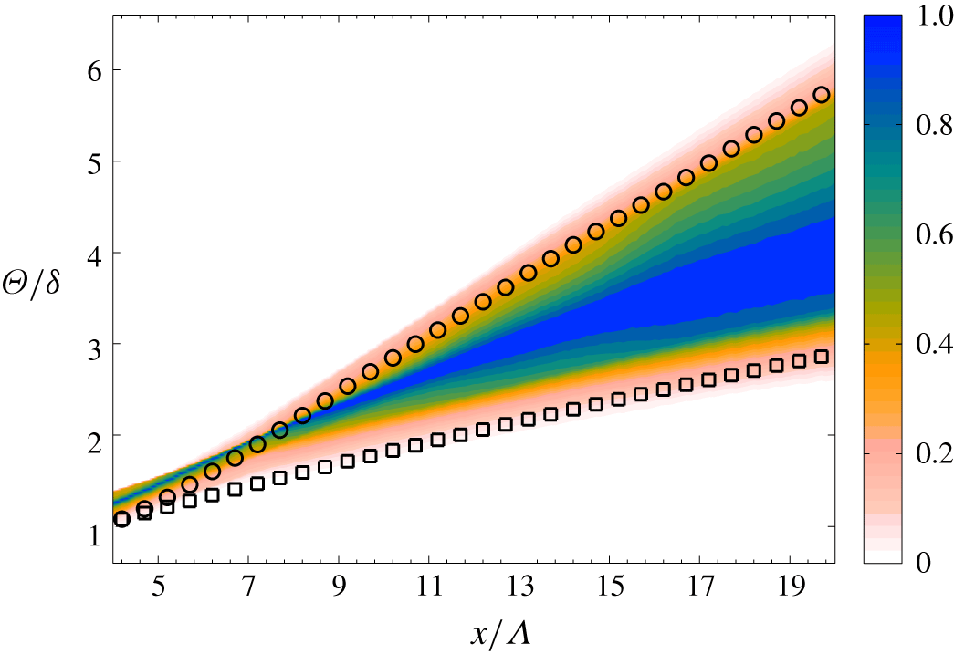
Normalized two-dimensional p.d.f. of the momentum thickness  $\unicode[STIX]{x1D6E9}$, obtained via gPC. Circle/square markers indicate results from the classical DNS for high/low
 $\unicode[STIX]{x1D6FC}$ value, respectively.

The first quantity investigated is the momentum thickness  $\unicode[STIX]{x1D6E9}$. The two-dimensional p.d.f. obtained for
 $\unicode[STIX]{x1D6E9}$ is shown in figure 9. What we refer to as two-dimensional p.d.f.s is actually an ensemble of one-dimensional p.d.f.s that are plotted together. For each of the streamwise sections previously introduced, a gPC analysis is performed and
 $3\times 10^{6}$ Monte Carlo samples are generated. From these samples, a smoothed p.d.f. is generated via a kernel smoothing function and all data are normalized over the peak of this distribution. The choice to perform such a normalization for each p.d.f. highlights the most probable configurations as a function of
 $x$ in the surface plot. However, considering that in this case
 $x$ does not have a probabilistic interpretation but is just a plot variable, some waviness of the p.d.f.s moving away from the most probable value can be observed. The gPC results are compared with those of the simulations of classical mixing-layer configurations (skew angle
 $\unicode[STIX]{x1D703}=0$,
 $\unicode[STIX]{x1D6FC}=0.66$ (round markers) and
 $\unicode[STIX]{x1D6FC}=0.23$ (square markers)). Figure 9 clearly shows that, upstream of
 $x\approx 5\unicode[STIX]{x1D6EC}$, occurrences of
 $\unicode[STIX]{x1D6E9}$ tend to cluster around values that are higher than the two classical simulations. As seen in § 4, this region is characterized by the presence and the evolution of coherent vortical structures generated at the inlet. In agreement with the analysis in § 4, lack of parallelism between the two asymptotic flows leads to a faster growth of these structures, and thus enhances mixing between the streams. These results are in agreement with stability analyses reported in the literature (Lu & Lele Reference Lu and Lele1993, Reference Lu and Lele1999a,Reference Lu and Leleb). However, the upstream region is characterized by a rather small variability of the momentum thickness (see also § 4).
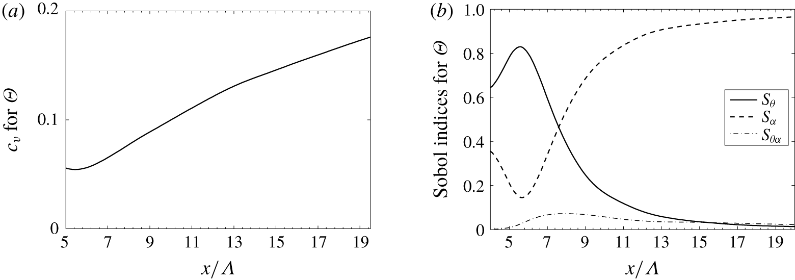
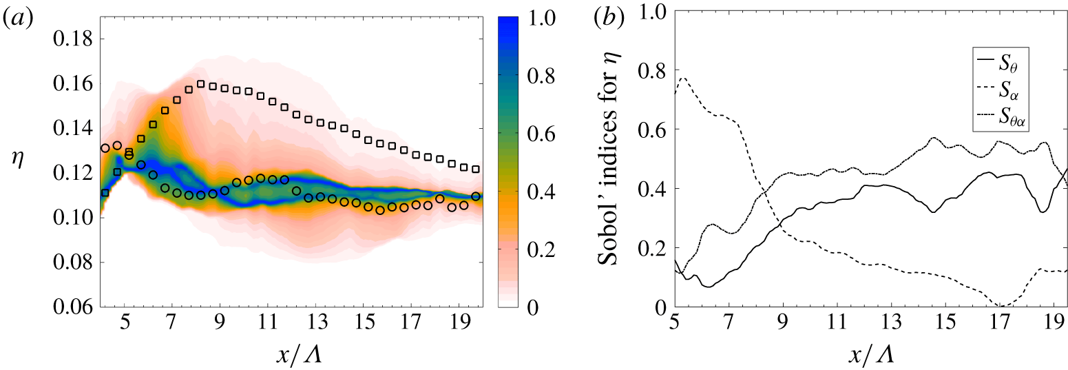
Similar conclusions can be drawn via analysis of the coefficient of variance  $c_{v}=|\unicode[STIX]{x1D6E9}^{\prime }/\overline{\unicode[STIX]{x1D6E9}}|$, which is reported in figure 10(a). Here
 $\unicode[STIX]{x1D6E9}^{\prime }$ is the standard deviation of
 $\unicode[STIX]{x1D6E9}$. Thus,
 $c_{v}$ provides an indication of the variance of the phenomenon investigated with respect to its mean value in the parameter space. For the quantities investigated, the mean value is usually very close to the most probable value shown in the two-dimensional p.d.f. in figure 9. The
 $c_{v}$ increases almost linearly from approximately 6 % to 18 % in the interval
 $x=5\unicode[STIX]{x1D6EC}$ to
 $x=19\unicode[STIX]{x1D6EC}$. The Sobol indices in figure 10(b), which provide a measure of the sensitivity of
 $\unicode[STIX]{x1D6E9}$ to each of the uncertainty parameters, confirm that the momentum thickness evolution in the upstream part of the mixing layer is mostly sensitive to
 $\unicode[STIX]{x1D703}$, even if the normalized variance indicated by
 $c_{v}$ is lower than towards the end of the investigation window. Moving downstream, the p.d.f. progressively shows a smoothed behaviour which encompasses the two classical simulations while the variance of
 $\unicode[STIX]{x1D6E9}$ increases almost linearly with
 $x/\unicode[STIX]{x1D6EC}$, as shown by the coefficient of variance in figure 10(a). Moreover, consistent with the observations in § 4, the effect of
 $\unicode[STIX]{x1D703}$ is progressively less intense as the flow transitions to fully developed turbulence. Inlet vortical structures lose coherence and the vorticity field exhibits a chaotic behaviour as the shear intensity
 $\unicode[STIX]{x1D6FC}$ becomes the dominant parameter. Finally, the interaction between the two parameters appears to be also minimal in this zone (
 $s_{\unicode[STIX]{x1D703}\unicode[STIX]{x1D6FC}}\approx 0$), indicating a clear separation of the dynamic effects.
Statistical properties of the momentum thickness  $\unicode[STIX]{x1D6E9}$, derived via stochastic analysis: (a) the coefficient of variance
 $c_{v}$ and (b) the Sobol indices.

Classical mixing layers are characterized by a so-called ‘self-similar’ region, in which the mean streamwise velocity profile in the normal direction, if properly rescaled, becomes invariant with  $x$ (see e.g. Pope Reference Pope2000). More precisely, the quantity
 $$\begin{eqnarray}\widetilde{U}=\frac{\overline{u_{x}}-{\textstyle \frac{1}{2}}\Vert \boldsymbol{U}_{1}+\boldsymbol{U}_{2}\Vert }{\Vert \boldsymbol{U}_{1}-\boldsymbol{U}_{2}\Vert }\end{eqnarray}$$
becomes independent of  $x$ if plotted as a function of the rescaled coordinate
 $\unicode[STIX]{x1D709}=(y-\unicode[STIX]{x1D6FF}_{U_{x}}(x))/x$, where
 $\unicode[STIX]{x1D6FF}_{U_{x}}(x)$ is the value of
 $y$ at which
 $\overline{u_{x}}=1/2\Vert \boldsymbol{U}_{1}+\boldsymbol{U}_{2}\Vert$ (McMullan et al. Reference McMullan, Gao and Coats2007). The distance from the inlet in the streamwise direction at which the self-similar region is completely established is mildly sensitive to the mixing-layer dynamics (parameter
 $\unicode[STIX]{x1D6FC}$). One could argue that, for higher
 $\unicode[STIX]{x1D6FC}$ values, intermittency and non-equilibrium of the flow should be more important, delaying the establishment of a complete self-similar state. The rate of convergence to a self-similar velocity profile is measured here using the following quantity:
 $$\begin{eqnarray}SS_{x}(x)=\frac{\displaystyle \left(\iint _{yz}(\widetilde{U}(x,\unicode[STIX]{x1D709})-\widetilde{U}(20\unicode[STIX]{x1D6EC},\unicode[STIX]{x1D709}))^{2}\,\text{d}\unicode[STIX]{x1D709}\right)^{0.5}}{\displaystyle \left(\iint _{yz}\widetilde{U}(20\unicode[STIX]{x1D6EC},\unicode[STIX]{x1D709})^{2}\,\text{d}\unicode[STIX]{x1D709}\right)^{0.5}},\end{eqnarray}$$
which is the  $L^{2}$ norm of the difference with respect to the
 $\widetilde{U}$ profile at the streamwise section
 $x=20\unicode[STIX]{x1D6EC}$, taken as a reference.
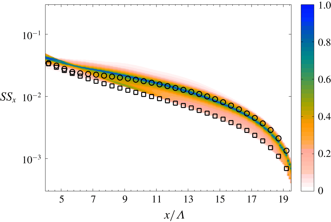
Normalized two-dimensional p.d.f. of the self-similarity indicator  $SS_{x}$, obtained via gPC. Circle/square markers indicate results from the classical DNS for high/low
 $\unicode[STIX]{x1D6FC}$ value, respectively.

Figure 11 shows the p.d.f. of  $SS_{x}$ as a function of the
 $x$ coordinate. It can be seen that most of the occurrences tend to cluster around the behaviour of the classical simulation, which has the lowest convergence rate, i.e. for higher
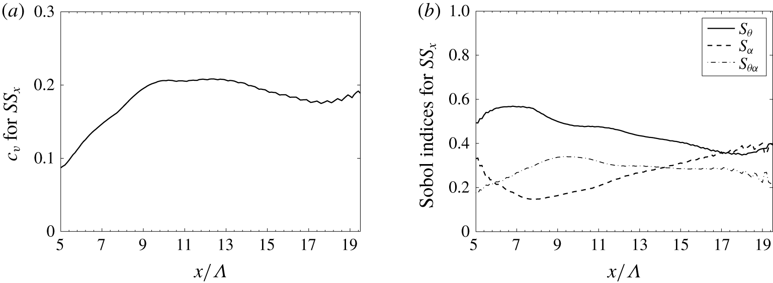
 $\unicode[STIX]{x1D6FC}$ value. However, the coefficient of variance shown in figure 12(a) is almost constant and very close to 20 % moving downstream, which indicates a non-negligible sensitivity of this quantity to the considered parameters. The analysis of the Sobol indices in figure 12(b) indicates that the sensitivity to the two parameters is similar and that there is a strong coupling between the effects of
 $\unicode[STIX]{x1D6FC}$ and
 $\unicode[STIX]{x1D703}$, resulting in a non-trivial response of this quantity in the parameter space.
Statistical properties of the self-similarity indicator  $SS_{x}$, derived via stochastic analysis: (a) the coefficient of variance
 $c_{v}$ and (b) the Sobol indices.

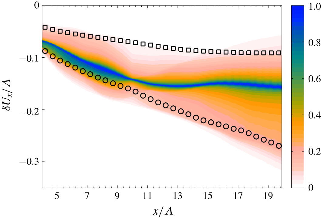
Classical mixing layers are characterized by an asymmetric growth with respect to the  $x$ axis due to the imbalance between the momentum of the two asymptotic flows, which pushes the mixing layer towards the lower-momentum region (Pope Reference Pope2000). A measure of this asymmetry is given by
 $\unicode[STIX]{x1D6FF}_{U_{x}}(x)$, previously defined. Figure 13 shows the p.d.f. of
 $\unicode[STIX]{x1D6FF}_{U_{x}}$ as a function of
 $x$, together with the behaviour obtained for classical mixing layers (
 $\unicode[STIX]{x1D703}=0$) for low and high values of
 $\unicode[STIX]{x1D6FC}$. As expected, for classical mixing layers,
 $\unicode[STIX]{x1D6FF}_{U_{x}}$ is significantly larger in magnitude for high
 $\unicode[STIX]{x1D6FC}$, due to the larger velocity difference between the streams (see table 1). The p.d.f. shows that in the upstream region most of the occurrences tend to cluster in proximity of the results for the high-
 $\unicode[STIX]{x1D6FC}$ classical simulation. This indicates that the presence of a skew angle enhances not only the growth of the mixing-layer thickness in this region, as previously observed in § 4 and from the momentum thickness behaviour, but also its displacement in the normal direction towards the slower stream, as can be qualitatively appreciated also from figure 7.
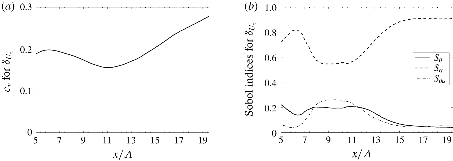
The Sobol indices in figure 14(b) confirm that in the upstream region, although  $\unicode[STIX]{x1D6FC}$ is the dominant parameter, there is a non-negligible influence of
 $\unicode[STIX]{x1D703}$, especially between
 $x\approx 7\unicode[STIX]{x1D6EC}$ and
 $11\unicode[STIX]{x1D6EC}$. In this region the impact of
 $\unicode[STIX]{x1D6FC}$ over the variance of
 $\unicode[STIX]{x1D6FF}U_{x}$ is not even 60 %, while the interaction between the two parameters accounts for up to 25 % of the total variation. One should consider that in this region the
 $c_{v}$ exhibits a minimum of approximately 17 % (see figure 14a). Moving downstream, the variance of
 $\unicode[STIX]{x1D6FF}U_{x}$ increases to
 $c_{v}\approx 28\,\%$, as the p.d.f. of
 $\unicode[STIX]{x1D6FF}_{U_{x}}$ is more spread and encompasses the values obtained for classical mixing layers for high and low
 $\unicode[STIX]{x1D6FC}$. As expected, the sensitivity to
 $\unicode[STIX]{x1D703}$ becomes negligible. Once again these results are consistent with the low impact of
 $\unicode[STIX]{x1D703}$ observed in the more downstream region for the mixing-layer growth (see § 4 and figure 10b).
Normalized two-dimensional p.d.f. of  $\unicode[STIX]{x1D6FF}_{U_{x}}$, obtained via gPC. Circle/square markers indicate results from the classical DNS for high/low
 $\unicode[STIX]{x1D6FC}$ value, respectively.

Statistical properties of the characteristic length  $\unicode[STIX]{x1D6FF}_{U_{x}}$, derived via stochastic analysis: (a) the coefficient of variance
 $c_{v}$ and (b) the Sobol indices.

5.1 Reynolds stress tensor
The stochastic analysis via gPC is now extended to the behaviour of the Reynolds stress tensor  $\overline{u_{i}^{\prime }u_{j}^{\prime }}$ and to the turbulent kinetic energy
 ${\mathcal{K}}=0.5(\overline{u_{x}^{\prime }u_{x}^{\prime }}+\overline{u_{y}^{\prime }u_{y}^{\prime }}+\overline{u_{z}^{\prime }u_{z}^{\prime }})$. Analysis of the simulations of the database indicates that the turbulence intensity in the mixing region (i.e.
 ${\mathcal{K}}/\Vert \boldsymbol{U}_{1}-\boldsymbol{U}_{2}\Vert ^{2}$) is approximately 3 %–10 %. The Reynolds stress tensor is an important indicator of the statistical properties of turbulence, and its sensitivity to parametric uncertainty can highlight the emergence of different physical mechanisms. The following quantities are investigated:
 $$\begin{eqnarray}\begin{array}{@{}rlrl@{}}\text{(i)}\ & K(x)=\displaystyle \iint _{yz}{\mathcal{K}}\,\text{d}y\,\text{d}z,\qquad & \text{(v)}\ & \overline{UV}(x)=\displaystyle \iint _{yz}\overline{u_{x}^{\prime }u_{y}^{\prime }}\,\text{d}y\,\text{d}z,\\ \text{(ii)}\ & \overline{UU}(x)=\displaystyle \iint _{yz}\overline{u_{x}^{\prime }u_{x}^{\prime }}\,\text{d}y\,\text{d}z,\qquad & \text{(vi)}\ & \overline{UW}(x)=\displaystyle \iint _{yz}\overline{u_{x}^{\prime }u_{z}^{\prime }}\,\text{d}y\,\text{d}z,\\ \text{(iii)}\ & \overline{VV}(x)=\displaystyle \iint _{yz}\overline{u_{y}^{\prime }u_{y}^{\prime }}\,\text{d}y\,\text{d}z,\qquad & \text{(vii)}\ & \overline{VW}(x)=\displaystyle \iint _{yz}\overline{u_{y}^{\prime }u_{z}^{\prime }}\,\text{d}y\,\text{d}z.\\ \text{(iv)}\ & \overline{WW}(x)=\displaystyle \iint _{yz}\overline{u_{z}^{\prime }u_{z}^{\prime }}\,\text{d}y\,\text{d}z,\qquad & \ & \end{array}\end{eqnarray}$$
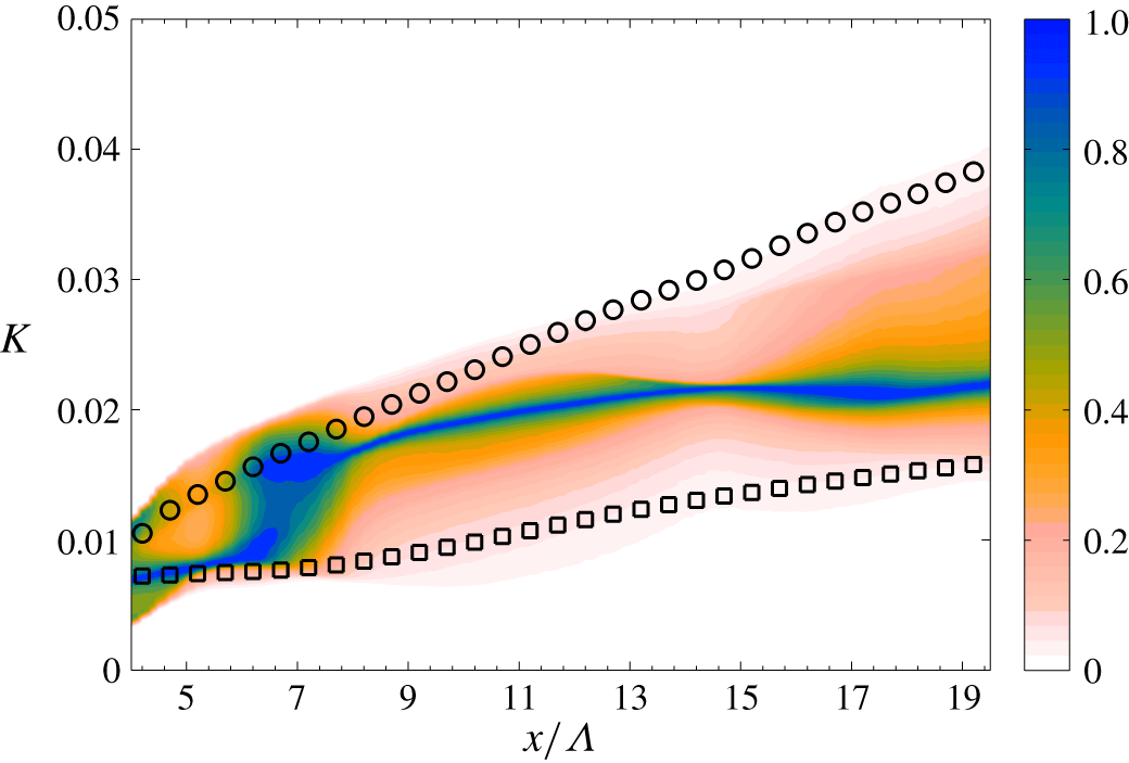
Normalized two-dimensional p.d.f. of the turbulent kinetic energy  $K$, obtained via gPC. Circle/square markers indicate results from the classical DNS for high/low
 $\unicode[STIX]{x1D6FC}$ value, respectively.

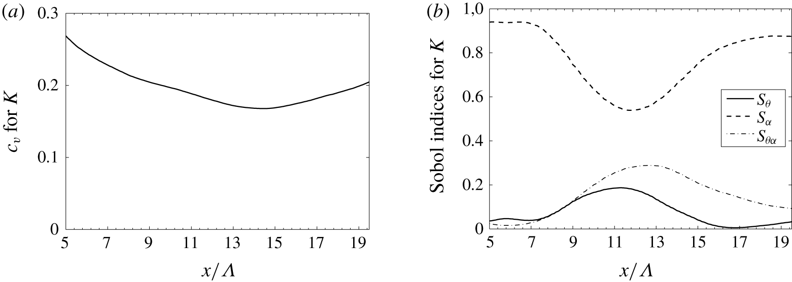
The evolution of the turbulent kinetic energy  $K$ is investigated in figure 15. It is possible to observe that, for
 $x\approx 8\unicode[STIX]{x1D6EC}$, the total turbulent kinetic energy tends to cluster around the high-
 $\unicode[STIX]{x1D6FC}$ classical configuration, i.e. the effects of the skew angle
 $\unicode[STIX]{x1D703}$ enhance the production of turbulent kinetic energy in the transition region. This feature becomes progressively less intense moving downstream, as turbulence forgets the initial instability mechanism and the interaction of the two asymptotic flows becomes more important. It is also interesting to observe similarities between this p.d.f. and the one in figure 13 for the wake displacement in the normal direction. Similar conclusions were drawn for that quantity. The analysis of the coefficient of variance
 $c_{v}$ and the Sobol indices in figure 16(b) confirms that, as for the quantity
 $\unicode[STIX]{x1D6FF}_{U_{x}}$, the parameter
 $\unicode[STIX]{x1D6FC}$ is governing before and after the transition, but that for
 $x\approx 10\unicode[STIX]{x1D6EC}$ the importance of
 $\unicode[STIX]{x1D6FC}$ and
 $\unicode[STIX]{x1D703}$ and in particular of their interaction is similar. In this case the influence of the interaction between the two parameters is even more relevant, as
 $c_{v}$ (shown in figure 16a) does not exhibit significant variations moving downstream. This observation reinforces the idea that small skew angles can actually be used to influence the physics of the transition to turbulence, which can provide new insights for the control of this class of flows.
Statistical properties of the turbulent kinetic energy  $K$, derived via stochastic analysis: (a) the coefficient of variance
 $c_{v}$ and (b) the Sobol indices.

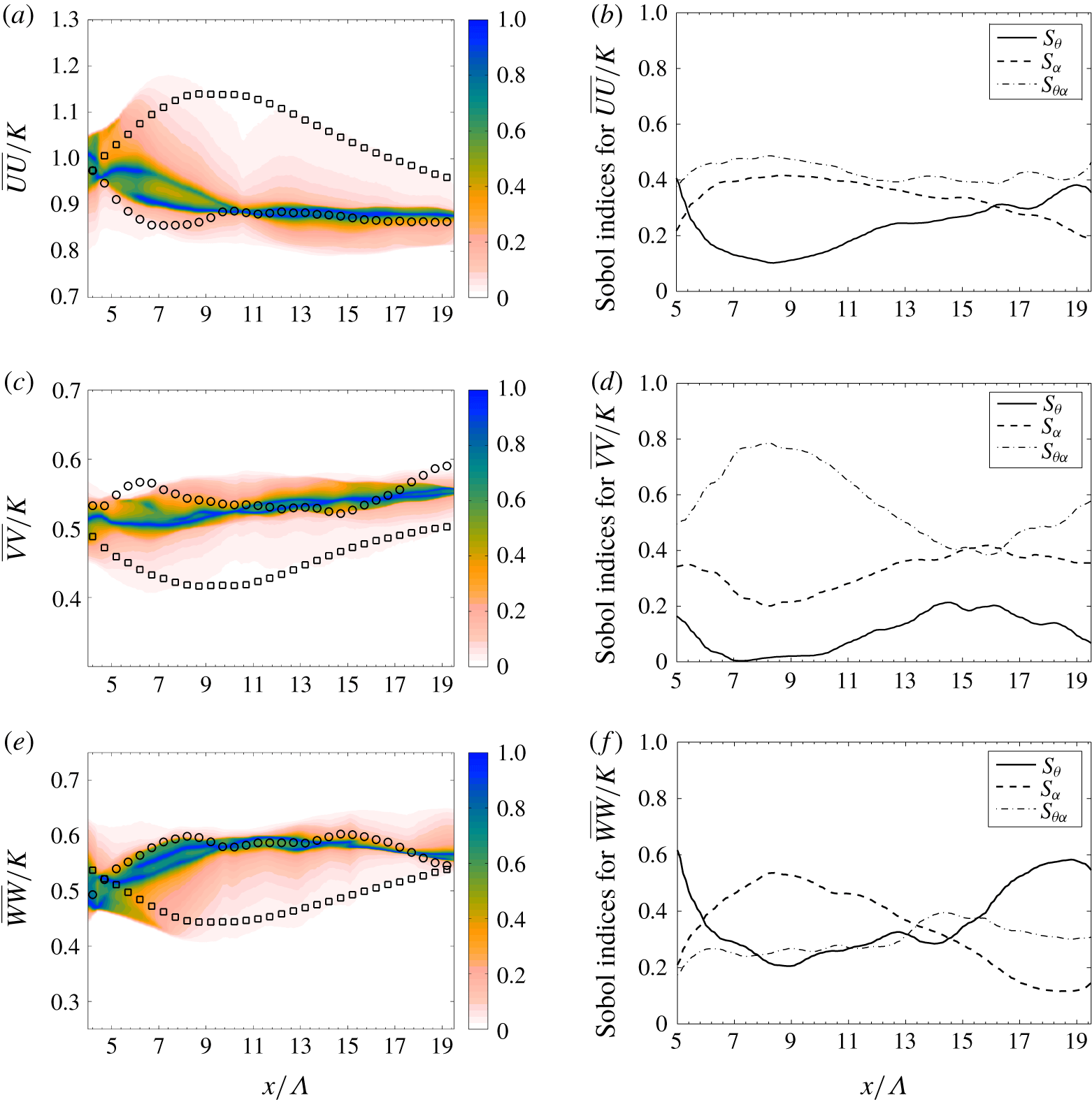
Statistical analysis of the diagonal elements of the Reynolds stress tensor, normalized over  $K$: (a,c,e) normalized two-dimensional p.d.f. and (b,d,f) Sobol indices, respectively. The quantities investigated are (a,b)
 $\overline{UU}/K$, (c,d)
 $\overline{VV}/K$ and (e,f)
 $\overline{WW}/K$. Circle/square markers indicate results from the classical DNS for high/low
 $\unicode[STIX]{x1D6FC}$ value, respectively.

When normalized over the total turbulent kinetic energy  $K$, the Reynolds stress tensor exhibits peculiar features. Two-dimensional p.d.f.s for
 $\overline{UU}$,
 $\overline{VV}$ and
 $\overline{WW}$ are shown in figure 17, along with the corresponding Sobol indices. One must keep in mind that, due to the normalization over
 $K$,
 $\overline{UU}+\overline{VV}+\overline{WW}=2$ for each streamwise section of each simulation. In this case, most of the occurrences for the three quantities cluster around the high-
 $\unicode[STIX]{x1D6FC}$ classical configuration. So, while the angle
 $\unicode[STIX]{x1D703}$ appears to have a localized effect over the distribution of
 $K$ and
 $\unicode[STIX]{x1D6FF}_{U_{x}}$, a global modification of the structure of the Reynolds stress tensor is observed. In particular, occurrences for
 $\overline{VV}$ and
 $\overline{WW}$ cluster around the
 $\unicode[STIX]{x1D703}=0$, high-
 $\unicode[STIX]{x1D6FC}$ behaviour and the mixing exhibits more isotropic features. However, it is also surprising to see that the contribution of
 $\unicode[STIX]{x1D703}$ and
 $\unicode[STIX]{x1D6FC}$ is much more similar for the components of the Reynolds stress tensor, and the way they interact is possibly the real governing element. The analysis of the coefficient
 $c_{v}$ shows that a peak for
 $c_{v}\approx 6\,\%{-}8\,\%$ for
 $x\approx 8\unicode[STIX]{x1D6EC}$ is observed for all three components. One can see that in this region
 $s_{\unicode[STIX]{x1D703}\unicode[STIX]{x1D6FC}}$ is important for
 $\overline{UU}/K$ and
 $\overline{WW}/K$ and it is the dominant index for
 $\overline{VV}/K$, where
 $s_{\unicode[STIX]{x1D6FC}\unicode[STIX]{x1D703}}\approx 0.8$. This last component of the Reynolds stress tensor is an indicator of the transition towards fully developed turbulence (Attili & Bisetti Reference Attili and Bisetti2012) and it was also analysed in § 4 in the region
 $x/\unicode[STIX]{x1D6EC}<4$.
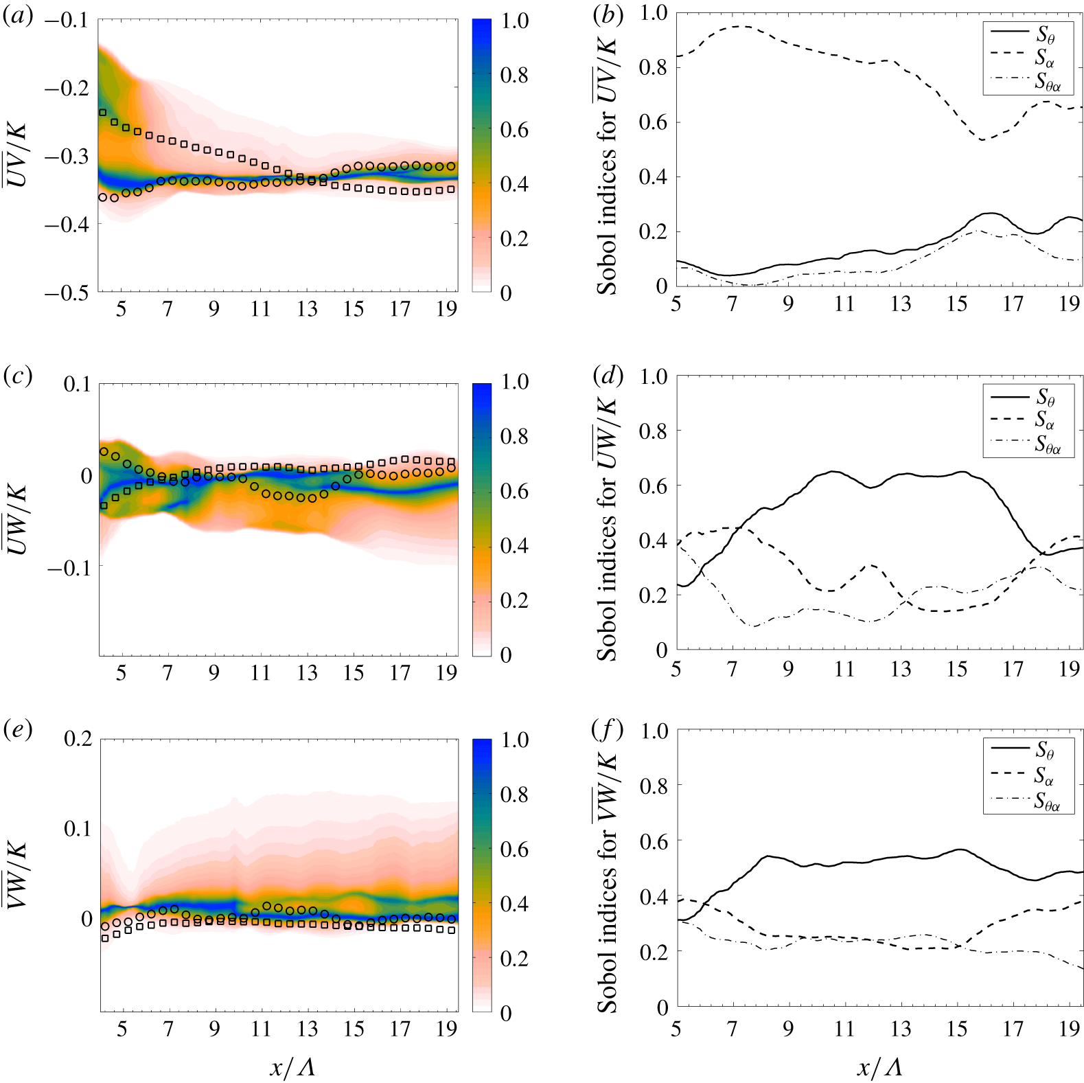
Important information can be deduced by the analysis of  $\overline{UV}$ in figure 18(a). This parameter is the true signature of turbulent shear effects for this test case. Considering that the shear-based Reynolds number is the same for every simulation of the database, one would expect to observe approximately the same value of this normalized quantity. This is true sufficiently downstream for
 $x>13\unicode[STIX]{x1D6EC}$. However, once again, most of the occurrences cluster around the high-
 $\unicode[STIX]{x1D6FC}$ classical configuration, showing that the presence of a skew angle can influence the nature of the turbulent state emerging by the interaction of the two asymptotic flows. However, the analysis of the Sobol indices in figure 18(b) indicates that the parameter
 $\unicode[STIX]{x1D6FC}$ is here more governing than in the other cases.
Finally, the two quantities  $\overline{UW}$ and
 $\overline{VW}$ are investigated. Normalized two-dimensional p.d.f.s are shown in figure 18(c,e). The simulations for
 $\unicode[STIX]{x1D703}=0$ exhibit almost zero values for these two quantities, indicating that production effects and pressure–strain interactions should be minimal for these cases. Small but non-zero values can be observed relatively upstream, which are associated with the complex inlet conditions applied (including non-zero average spanwise velocity). However, one can clearly see that the two components tend to zero sufficiently downstream. While most of the occurrences of the database tend to cluster around the classical configurations, a non-negligible part exhibits negative values for
 $\overline{UW}$ and positive values for
 $\overline{VW}$. Arguably, the analysis of these components of the tensor could more clearly highlight the presence of a bias in the direction of the co-flows, if parallelism is imposed or expected.
Also, the analysis of the Sobol indices in figure 18(d,f) indicates that, for these physical quantities,  $\unicode[STIX]{x1D703}$ is the governing parameter, consistent with previous discussion. Similar conclusions are drawn in the stability analysis by Lu & Lele (Reference Lu and Lele1999a) and in a numerical study for the backward-facing step flow by Kaltenbach (Reference Kaltenbach2003). In both analyses, it is stressed that turbulence production associated with the spanwise shear effect provides a significant amount of disturbance energy, which is responsible for the increase in the amplification rate for the growth of the mixing layer.
Statistical analysis of the diagonal elements of the Reynolds stress tensor, normalized over  $K$: (a,c,e) normalized two-dimensional p.d.f. and (b,d,f) Sobol indices, respectively. The quantities investigated are (a,b)
 $\overline{UU}/K$, (c,d)
 $\overline{VV}/K$ and (d,f)
 $\overline{WW}/K$. Circle/square markers indicate results from the classical DNS for high/low
 $\unicode[STIX]{x1D6FC}$ value, respectively.

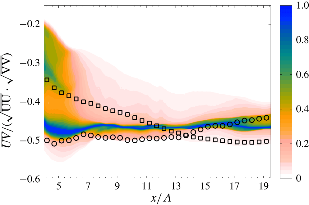
A qualitative discussion about the parameter  $\overline{UV}/\big(\sqrt{\overline{UU}}\,\sqrt{\overline{VV}}\big)$ is now provided. This parameter is widely used in the analysis of turbulent sheared flows and its value is approximately
 $-0.5$ (Champagne, Harris & Corrsin Reference Champagne, Harris and Corrsin1970). The two-dimensional p.d.f. of this parameter is provided in figure 19. One can see that for
 $x>7\unicode[STIX]{x1D6EC}$ (i.e. after the initial stages of transition towards turbulence) the parameter is included in the range
 $[-0.5,-0.4]$ for every simulation of the database. However, the classical DNS for lower
 $\unicode[STIX]{x1D6FC}$ exhibits a significantly slower convergence towards the asymptotic limit, due to the less intense mixing effect. On the other hand, most of the occurrences calculated via gPC cluster around the red circles for
 $x<13\unicode[STIX]{x1D6EC}$, proving again that the lack of parallelism between the two flows enhances mixing capacities. For
 $x>15\unicode[STIX]{x1D6EC}$ the gPC prediction becomes more homogeneous in the range
 $[-0.5,-0.42]$, which are the asymptotic values exhibited by the two classical configurations investigated.
Two-dimensional p.d.f. of the shear parameter  $\overline{UV}/\big(\sqrt{\overline{UU}}\,\sqrt{\overline{VV}}\big)$, obtained via uncertainty propagation using a gPC–DNS tool.

At last, the anisotropy of the Reynolds stress tensor is investigated (Tennekes & Lumley Reference Tennekes and Lumley1972; Hamilton & Bayoan Cal Reference Hamilton and Bayoan Cal2015). This quantity is obtained via manipulation of the matrix:
 $$\begin{eqnarray}\unicode[STIX]{x1D622}_{ij}=\frac{\overline{u_{i}^{\prime }u_{j}^{\prime }}}{2{\mathcal{K}}}-\frac{1}{3}\unicode[STIX]{x1D6FF}_{ij}.\end{eqnarray}$$
The calculation of the eigenvalues  $\unicode[STIX]{x1D706}_{i}$ of the matrix
 $\unicode[STIX]{x1D622}_{ij}$ provides the value of the anisotropy
 $\unicode[STIX]{x1D702}$ as
 $$\begin{eqnarray}\unicode[STIX]{x1D702}^{2}={\textstyle \frac{1}{3}}(\unicode[STIX]{x1D706}_{1}^{2}+\unicode[STIX]{x1D706}_{1}\unicode[STIX]{x1D706}_{2}+\unicode[STIX]{x1D706}_{2}^{2}).\end{eqnarray}$$
For isotropic turbulence,  $\unicode[STIX]{x1D702}=0$ and larger values indicate a higher anisotropy of the Reynolds stress tensor. In this test case, the value of
 $\unicode[STIX]{x1D702}$ is expected to tend to zero moving downstream, as turbulence exhibits a progressive return to isotropy. For each simulation, the anisotropy is calculated at the centre of the mixing layer, i.e. at the distance
 $-\unicode[STIX]{x1D6FF}_{U_{x}}(x)$ from the centreline
 $y=0$. The response surface reconstructed via gPC is shown in figure 20(a). The coefficient of variance
 $c_{v}$ for this quantity shows an almost constant value
 $c_{v}\approx 0.13$ in the range
 $7\leqslant x/\unicode[STIX]{x1D6EC}\leqslant 13$ before a linear decrease to a value of
 $c_{v}=0.05$ for
 $x/\unicode[STIX]{x1D6EC}=20$. In agreement with the analyses previously reported, most of the occurrences generated via gPC tend to cluster around the predicted
 $\unicode[STIX]{x1D702}$ for the classical DNS for higher
 $\unicode[STIX]{x1D6FC}$. This behaviour is a result of the enhanced mixing due to the skew angle
 $\unicode[STIX]{x1D703}$. Similar information is deduced from the analysis of the Sobol indices in figure 20(b). The shear intensity parameter
 $\unicode[STIX]{x1D6FC}$ is a governing parameter only for
 $x/\unicode[STIX]{x1D6EC}<8$, while
 $s_{\unicode[STIX]{x1D703}}+s_{\unicode[STIX]{x1D703}\unicode[STIX]{x1D6FC}}>0.8$ in the rest of the physical domain.
Anisotropy of the Reynolds stress tensor  $\unicode[STIX]{x1D702}$, obtained via uncertainty propagation using a gPC–DNS tool. This quantity is sampled at the centre of the wake. (a) The normalized two-dimensional p.d.f. and (b) the Sobol indices are shown, respectively.

6 Conclusions
A sensitivity analysis of DNS of the turbulent spatially evolving mixing layer has been performed. The effects of the shear parameter  $\unicode[STIX]{x1D6FC}$ and the skew angle
 $\unicode[STIX]{x1D703}$ measuring the lack of parallelism between the two flows over the physical features of the flow have been investigated. The choice of the parameters for the present investigation is performed with the objective to enhance the physical understanding of the considered flow features. This opens perspectives of application towards flow control, and reliable comparison between experiments, simulations and turbulence modelling. A database of 18 DNS has been used to perform the analysis, which encompassed observation of structural features as well as stochastic characterization of time-averaged quantities. The latter has been developed via response surface reconstruction using gPC.
The analysis of instantaneous and time-averaged flow features of the DNS of the database indicates that variations of the parameter  $\unicode[STIX]{x1D6FC}\in [0.2,0.7]$ has a primary effect on the growth of the mixing region. This is associated with shear effects due to the interaction of the co-flows, following the known mechanisms of classical mixing layers. A secondary effect associated with
 $\unicode[STIX]{x1D703}$ is observed as well. Higher values for the skew angle are responsible for a rapid increase of the growth of inlet structures, enhancing the development of the mixing region. This effect is associated with an increase of the cross-wise velocity fluctuation energy. However, this effect is hidden by bulk shear interactions for higher
 $\unicode[STIX]{x1D6FC}$ values.
The analysis of statistical features of the time-averaged velocity field, such as the momentum thickness  $\unicode[STIX]{x1D6E9}$, provides consistent results with the previous investigation. Additionally, the response surface reconstruction allows for a precise quantification of the effects of each parameter, as well as of the total variation rate in the parametric range investigated. Again, the parameter
 $\unicode[STIX]{x1D6FC}$ completely governs dynamics associated with the time-averaged velocity field in the fully developed turbulence region, while the effects of the parameter
 $\unicode[STIX]{x1D703}$ are not negligible in the inlet/transition region. In addition, the effects of the two parameters are mainly independent for these physical quantities.
Interesting results are observed via stochastic analysis of the Reynolds stress tensor, which describes the features of the turbulent field. While the behaviour of the integrated turbulent kinetic energy  $K$ is similar to the time-averaged quantity
 $\unicode[STIX]{x1D6FF}_{U_{x}}$ (i.e. governing effects of
 $\unicode[STIX]{x1D6FC}$ downstream), a global modification of the normalized diagonal components of the Reynolds stress tensor due to
 $\unicode[STIX]{x1D703}$ is observed. In particular, occurrences for
 $\overline{VV}$ and
 $\overline{WW}$ cluster around the
 $\unicode[STIX]{x1D703}=0$, high-
 $\unicode[STIX]{x1D6FC}$ behaviour and the mixing exhibits more isotropic features. In addition, the interaction between the parameters
 $\unicode[STIX]{x1D703}$ and
 $\unicode[STIX]{x1D6FC}$ is here the governing element. Similar conclusions can be deduced for the behaviour of the normalized component of the Reynolds stress tensor
 $\overline{UV}$ and the anisotropy
 $\unicode[STIX]{x1D702}$. These two quantities are indicators of the turbulent shear effect and of the mixing efficiency for this test case.
Future work envisions the investigation of the effects of the skew angle in combination with different inlet perturbations, in particular for the initial development of the mixing layer. The impact of variations of the Reynolds number could also be addressed.
Declaration of interests
The authors report no conflict of interest.
Appendix A. Validation of the DNS results and of the gPC strategy
In this section the validation of the numerical techniques employed in this work is provided. First, DNS results are investigated. The mesh resolution employed is the same as that proposed by Delport et al. (Reference Delport, Baelmans and Meyers2011) for the same inlet Reynolds number. Considering the size of the physical domain investigated ( $24\unicode[STIX]{x1D6EC}\times 15\unicode[STIX]{x1D6EC}\times 6\unicode[STIX]{x1D6EC}$), this results in
 $384\times 163\times 160$ mesh elements in the streamwise direction
 $x$, in the normal direction
 $y$ and in the spanwise direction
 $z$, respectively. The size of the mesh elements is homogeneous in the directions
 $x$ and
 $z$. More precisely, one characteristic length
 $\unicode[STIX]{x1D6EC}$ is discretized into
 $384/24=16$ mesh elements in the streamwise direction and in
 $160/6=26.67$ elements in the spanwise direction. In the normal direction
 $y$, elements are refined at the centreline and their resolution is coarsened moving towards the upper and lower traction-free boundary conditions. The rate of coarsening increases moving away from the centreline, while the size of the elements is almost constant in the range
 $-\unicode[STIX]{x1D6EC}<y<\unicode[STIX]{x1D6EC}$.
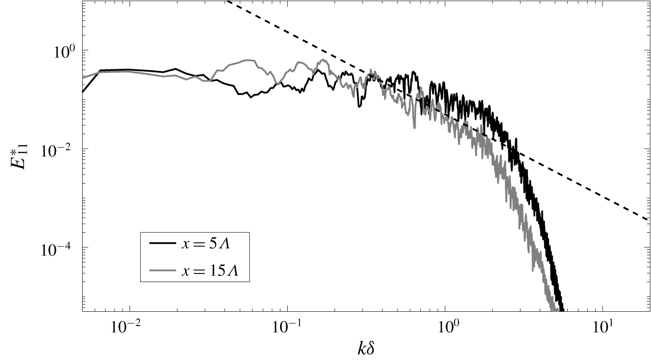
Normalized one-dimensional energy spectra  $E_{11}^{\star }=E_{11}/(\Vert \boldsymbol{U}_{1}-\boldsymbol{U}_{2}\Vert ^{2}\unicode[STIX]{x1D6FF})$. The spectra have been sampled for
 $y=0$,
 $z=0$ at the streamwise stations
 $x=5\unicode[STIX]{x1D6EC}$ and
 $x=15\unicode[STIX]{x1D6EC}$. Results shown are taken from the simulation for
 $\unicode[STIX]{x1D703}=0$,
 $\unicode[STIX]{x1D6FC}=0.666$.

The accuracy in the representation of turbulent features is assessed calculating the one-dimensional energy spectra for the streamwise fluctuating velocity  $E_{11}$. The spectra are shown in figure 21 for sensors positioned at the stations
 $[x,y,z]=[5,0,0]$ and
 $[x,y,z]=[15,0,0]$ in
 $\unicode[STIX]{x1D6EC}$ units. Results for the simulation
 $\unicode[STIX]{x1D703}=0$,
 $\unicode[STIX]{x1D6FC}=0.666$ are presented. The spectra show convincing results for the accurate representation of physical features such as a well-developed dissipative range as well as an increase of the Kolmogorov scale
 $\unicode[STIX]{x1D702}_{K}$ moving downstream. For the spectrum sampled at the streamwise station
 $x=15\unicode[STIX]{x1D6EC}$, one can clearly observe a scaling range of almost one decade proportional to
 $k^{-5/3}$. This result is consistent with the Reynolds number and the boundary conditions imposed at the inlet.
The strategy used in the present work to reconstruct the response surfaces via gPC is now assessed. The validation is performed comparing results obtained via a second-order ( $P=2$) and third-order (
 $P=3$) truncation of the polynomial expansion. This implies that the response surfaces for the investigated quantities are reconstructed using six and 10 polynomials, respectively. As an example, results for the quantity
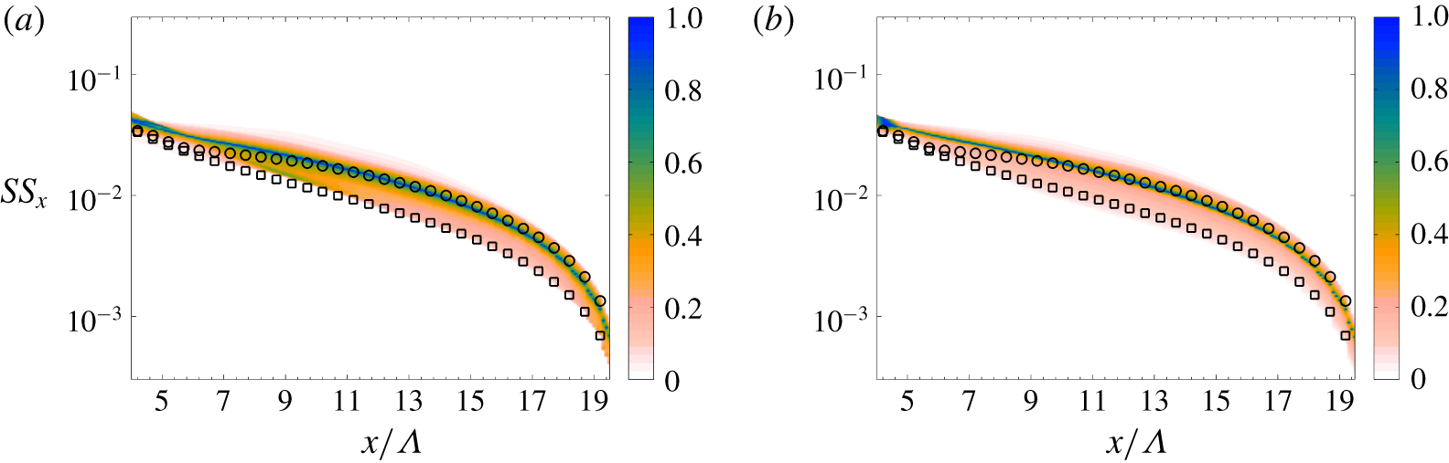
 $SS_{x}$ are reported in figure 22, whereas similar results are found for the other quantities of interest (not shown herein for the sake of brevity). No significant difference can be observed when comparing the gPC response surface for
 $P=2$ and
 $P=3$. This implies that convergence has been reached for
 $P=3$, which is the order of truncation of the polynomial expansion used in the present work.
Two-dimensional p.d.f. of the response surfaces calculated for the self-similarity parameter  $SS_{x}$. The response surfaces have been obtained using the gPC method truncating the polynomial expansion to (a) second order and (b) third order.