





Introduction
Diversification stands at the heart of the principles guiding agricultural transitions toward sustainability (Kremen and Miles, Reference Kremen and Miles2012; Tittonell, Reference Tittonell2014; Garibaldi et al., Reference Garibaldi, Aguiar, Aizen, Morales and Sáez2017). It refers to the intentional addition of functional biodiversity to agricultural systems, at multiple spatial and/or temporal scales (Kremen, Iles and Bacon, Reference Kremen, Iles and Bacon2012). Several studies show that enhancing biodiversity in agroecosystems increases long-term productivity while reducing dependence on synthetic inputs and cropland expansion (Garibaldi et al., Reference Garibaldi, Carvalheiro, Vaissière, Gemmill-Herren, Hipólito, Freitas, Ngo, Azzu, Sáez, Åström, An, Blochtein, Buchori, García, Da Silva, Devkota, Ribeiro and Freitas2016; Tamburini et al., Reference Tamburini, Bommarco, Wanger, Kremen, van der Heijden, Liebman and Hallin2020; Beillouin et al., Reference Beillouin, Ben-Ari, Malézieux, Seufert and Makowski2021). Yet, despite the recognition of the need for a multifaceted approach, sustainable agriculture research has predominantly concentrated on ecological facets (Rasmussen et al., Reference Rasmussen, Grass, Mehrabi, Smith, Bezner-Kerr, Blesh, Garibaldi, Isaac, Kennedy, Wittman, Batáry, Buchori, Cerda, Chará, Crowder, Darras, DeMaster, Garcia and Gómez2024). The interplay between ecological management, such as diversification of crops, and socioeconomic processes and outcomes remains inadequately explored, with economic impacts receiving even less attention. Moreover, the literature on the economic benefits of crop diversification remains limited, leaving important gaps in our understanding of how diversification affects farm income, risk, and overall economic sustainability.
Economic planning in agriculture is inherently intricate, and the degree of complexity is even higher in diversified farming systems. Farmers face multiple interrelated decisions, including crop selection, planting and harvesting schedules, the allocation of labor and capital, and the management of uneven cash flows, as expenditures and revenues occur at different moments of the production cycle. These decisions are highly interdependent (Bowman and Zilberman, Reference Bowman and Zilberman2013). In diversified systems, where several crops may overlap in space and time, these interactions create a dynamic and sometimes unpredictable environment (Prokopy et al., Reference Prokopy, Floress, Klotthor-Weinkauf and Baumgart-Getz2008; Hoshide, Reference Hoshide2023).
Many farmers’ decisions are based on experience, intuition, or historical practices rather than formal economic analysis. While experiential knowledge effectively guides farmers’ day-to-day management, it rarely provides systematic information on costs, revenues, and risks that could support more structured economic planning. Although agricultural research has developed decision-support tools to address this gap, these tools are often underutilized because they fail to adequately incorporate farmers’ local knowledge, context-specific practices, and on-the-ground constraints (Haraway, Reference Haraway1988; Altieri and Nicholls, Reference Altieri and Nicholls2005; Von Diest et al., Reference Von Diest, Wright, Samways and Kieft2020).
Economic sustainability in diversified systems
The economic dimension of agricultural sustainability is commonly framed in terms of long-term farm viability and is typically conceptualized around three core components: profitability, liquidity, and stability (Latruffe et al., Reference Latruffe, Diazabakana, Bockstaller, Desjeux, Finn, Kelly, Ryan and Uthes2016; Roesch et al., Reference Roesch, Gaillard, Isenring, Jurt, Keil, Nemecek, Rufener, Schüpbach, Umstätter, Waldvogel, Walter and Werner2017; Zorn et al., Reference Zorn, Esteves, Baur and Lips2018). In practice, these dimensions are operationalized through financial indicators derived from farm accounting data. As discussed by Buckwell et al. (Reference Buckwell, Nordang Uhre, Williams, Poláková, Blum, Schiefer, Lair, Heissenhuber, Schieβl, Krämer and Haber2014), numerous indicators have been proposed to assess the economic dimension of sustainability, reflecting both the richness and the methodological fragmentation of existing approaches. Assessing the economic sustainability of diversified farming systems is particularly challenging, as crops differ in their biological cycles, input requirements, and revenue streams. As a result, farm performance depends not only on aggregate outputs and annual profits but also on the timing and coordination of costs, revenues, and reinvestment opportunities across multiple activities. These temporal interactions are difficult to capture using conventional end-of-period indicators, which often overlook the dynamic nature of diversified production systems.
Some studies have addressed this complexity through the lens of risk diversification theory. O’Hara (Reference O’Hara2012) observes that crop diversification functions as a self-managed risk mitigation strategy: while adverse events—price shocks, pest outbreaks, or weather disruptions—can eliminate revenue in a specialized system, their impact on a diversified farm is contained to the affected crops, leaving others intact. Consistent with this argument, Burbano-Figueroa et al. (Reference Burbano-Figueroa, Sierra-Monroy, David-Hinestroza, Whitney, Borgemeister and Luedeling2022) and Paut, Sabatier and Tchamitchian (Reference Paut, Sabatier and Tchamitchian2019) apply Modern Portfolio Theory and decision analysis under uncertainty to evaluate crop diversification strategies. Their findings show that diversification can reduce income volatility by spreading risk across crops with different price and yield dynamics, thereby enhancing farm-level economic stability.
While these studies emphasize the role of diversification in reducing risk, the economic performance of small-scale diversified farms is also shaped by financial constraints that affect their liquidity and investment capacity. In many contexts, access to formal agricultural credit is limited, particularly for smallholders who often require relatively small loan amounts but face disproportionately high transaction costs and repayment structures that are poorly aligned with agricultural production cycles (Khan et al., Reference Khan, Nouman, Negrut, Abban, Cismas and Siddiqi2024). Under these conditions, the timing and availability of financial resources become critical determinants of farm performance, influencing farmers’ ability to cover production costs, sustain operations, and reinvest in subsequent production cycles.
Despite the importance of these financial dynamics, relatively little attention has been paid to how diversification affects the circulation of capital within farming systems. Most economic analyses focus on annual income, profitability, or risk reduction, while paying less attention to the temporal organization of costs, revenues, and reinvestment flows. In this study, we conceptualize crops not only as sources of yield and income but also as components of a dynamic capital system. Within this perspective, each crop generates returns that become available for reinvestment at different points of time in the cropping cycle, contributing to the circulation of capital within the farm. This approach allows us to explore additional benefits of diversification that emerge from the temporal distribution of costs and revenues. To this end, we present an economic analysis that isolates the effect of crop diversification from other agronomic and market-related factors, using the Profit Impact Simulator for Horticultural Farms (SIGCHA, from its Spanish acronym-Simulador de Impacto Ganancial para la Chacra Horticola). SIGCHA is specifically designed to model these interactions and translate complex dynamics into a set of key economic indicators, making it particularly well suited to the analysis of diversified agricultural systems.
Marketing of diverse crops
As farmers transition toward more diversified production systems, they often move away from conventional marketing structures based on selling large volumes of standardized products in integrated commodity markets. Instead of relying on intermediaries that purchase homogeneous products in bulk, diversified farmers must develop multiple marketing channels capable of handling smaller and more heterogeneous volumes. This shift increases logistical complexity, transaction costs, and the need for sustained investments in communication, promotion, and administrative management, leading to higher commercialization expenses (Dumont et al., Reference Dumont, Vanloqueren, Stassart and Baret2016; Chappell et al., Reference Chappell, Bernhart, Bachmann, Gonçalves, Seck, Nandula and Cristo dos Santos2018).
For diversified agriculture to develop, innovation must extend beyond technological and agronomic practices at the farm level to include social, economic, and institutional arrangements across local supply chains (Duru, Therond and Fares, Reference Duru, Therond and Fares2015; Tittonell, Reference Tittonell2019). In this context, short food supply chains (SFSCs) have emerged as a conceptual framework. By reducing the distance between farmers and consumers and limiting intermediaries, SFSCs allow farmers to capture higher prices and maintain greater control over the destination of their products, potentially improving the economic valorization of ecologically sustainable production (Chiffoleau, Millet-Amrani and Canard, Reference Chiffoleau, Millet-Amrani and Canard2016; Doernberg et al., Reference Doernberg, Piorr, Zasada, Wascher and Schmutz2022; Mengoni, Belletti and Marescotti, Reference Mengoni, Belletti and Marescotti2025). One rapidly expanding form of SFSC is community-supported agriculture (CSA). In CSA schemes, consumers make an upfront financial commitment in exchange for a share of the farm’s future harvest. Originally developed in Japan in the 1960s, CSA was introduced in North America and Europe during the 1980s and has since expanded to multiple continents (Cone and Myhre, Reference Cone and Myhre2000; Volz et al., Reference Volz, Weckenbrock, Cressot and Parot2016; Tian et al., Reference Tian, Zhang, Wang, Kang and Yang2024). CSA initiatives are now present in diverse cultural and socioeconomic contexts, including in Latin America, where they are developed alongside agroecological movements and adapted to local conditions (González-Azcárate et al., Reference González-Azcárate, Silva, Cruz-Maceín, López-García and Bardají2023).
In Argentina, CSA initiatives typically take the form of agroecological vegetable box schemes, in which local consumers purchase a weekly selection of seasonal produce. The upfront commitment typically takes the form of an advance payment by consumers at the beginning of the cropping season, locally referred to as pre-venta (‘pre-sale’). These advance payments provide liquidity to the farm at the time of purchasing production inputs, and have become a practice aimed at reducing risk and increasing liquidity in the context of the persistent economic instability and uncertainty in Argentina. However, systematic information on participation levels, economic performance, and organizational characteristics remains limited, making it difficult to assess the scale and economic significance of these initiatives in the Argentine context.
Although CSA models vary across institutional and socioeconomic contexts, they share a common feature: the establishment of long-term partnerships between farmers and consumers based on trust and shared commitments (Cone and Myhre, Reference Cone and Myhre2000; Volz et al., Reference Volz, Weckenbrock, Cressot and Parot2016). Through these arrangements, consumers share both the risks and rewards of agricultural production, reducing farmers’ exposure to market uncertainty and demand fluctuations (Cone and Myhre, Reference Cone and Myhre2000; Ostrom, Reference Ostrom, Hinrichs and Lyson2007). This risk-sharing function may be particularly relevant for diversified vegetable farmers, who often face structural barriers in accessing conventional crop insurance products designed for commodity crops (Belasco and Fuller, Reference Belasco and Fuller2022). More broadly, the literature suggests that these arrangements can strengthen farm resilience and support farmer livelihoods by creating more predictable economic conditions than those associated with conventional market channels (Ostrom, Reference Ostrom, Hinrichs and Lyson2007; Matzembacher and Meira, Reference Matzembacher and Meira2019).
Despite these expected economic benefits, empirical evidence on the economic performance of CSA farms remains mixed. While some studies report enhanced income stability and greater economic security associated with guaranteed markets and member commitments, others report persistent economic challenges among CSA farmers. Research from the United States and Europe has highlighted relatively low incomes, long working hours, and recurring patterns of self-exploitation, whereby farmers accept below-market returns in order to uphold social commitments and maintain the viability of the CSA model (Galt, Reference Galt2013; Paul, Reference Paul2019). Additional challenges include difficulties in member recruitment and retention, which may undermine the stability that CSA arrangements are intended to provide (Sulistyowati et al., Reference Sulistyowati, Afiff, Baiquni and Siscawati2023; Schmidt et al., Reference Schmidt, Egli, Gaspers, Zech, Gastinger and Rommel2025). As a result, the economic implications of CSA participation appear more complex than theoretical accounts of risk sharing and guaranteed markets alone would suggest.
Yet, there is still limited quantitative evidence regarding the mechanisms through which CSA participation affects farm economic performance. Existing studies have largely focused on outcomes such as income stability, farmer livelihoods, or organizational challenges, while paying comparatively little attention to the dynamics of financial processes through which CSA arrangements influence farm viability. In particular, little attention has been given to how preseason payments affect liquidity, capital requirements, and the circulation of financial resources within diversified farms. By shifting a portion of farm revenues to the beginning of the production cycle, CSA arrangements alter the temporal structure of financial flows within farming systems. However, such effects remain largely overlooked by conventional evaluation approaches, which typically focus on end-of-period outcomes and therefore fail to capture the temporal dimension of farm finances. Understanding these dynamics is particularly important given that economic factors remain one of the main barriers to the adoption of sustainable agricultural practices (Ansari and Tabassum, Reference Ansari and Tabassum2018; Coulibaly, Du and Diakité, Reference Coulibaly, Du and Diakité2021; Feliciano, Reference Feliciano2022). Robust evidence on the economic outcomes of diversification and alternative marketing strategies is therefore essential to support farmers’ decision-making processes.
This study analyzes the economic implications of crop diversification and alternative marketing strategies in horticultural systems in Northern Patagonia, Argentina. Using production and marketing data from three farms involved in a PAR process, we examine how diversification and participation in CSA schemes shape farm financial performance. Specifically, we address two research questions: (1) Is crop diversification economically beneficial? (2) How does participation in CSA schemes affect the financial structure and economic viability of diversified farms? To answer these questions, we simulate diversified farm management systems that integrate both productive and financial components in order to capture interactions between cropping strategies, cash-flow timing, and farm-level economic outcomes.
Research methods
SIGCHA: Profit impact simulator for horticultural farms
The economic analysis was conducted using SIGCHA, an economic planning and simulation tool designed to evaluate the dynamic effects of agronomic and economic decisions at the farm level. Developed in Argentina by the Coceplad Worker Cooperative (https://sigcha.streamlit.app/) in close collaboration with farmers, SIGCHA integrates production and financial information to assess how variations in key technical and economic parameters affect the overall economic performance of horticultural systems.
SIGCHA operationalizes a dynamic capital-turnover model developed in prior research, which conceptualizes production as a temporally structured process of capital commitment and recovery (Levín and Kicillof, Reference Levín and Kicillof1999; Romero and Benchimol, Reference Romero and Benchimol2008; Bonelli, Reference Bonelli2015; Etcheberry Mason and Bonelli, Reference Etcheberry Mason and Bonelli2015). At its core, the model reconstructs the chronological sequence of cash inflows and outflows of an enterprise. By assigning a precise time reference to each economic transaction, the model identifies the temporal structure of capital within the production cycle, referred to as its chronostructure. From this chronological reconstruction, the model’s dependent variables are derived: Committed Capital, Turnover Velocity, and Profit Rate. Together, these indicators provide a dynamic representation of economic performance grounded in the temporal configuration of cash flows.
The concept of Committed Capital is the central innovation of the SIG framework. It refers to the portion of capital that cannot be covered by revenues generated within the same period of analysis. In other words, when expenses exceed internally generated funds during the period under review, additional financing is required to sustain operations. Committed capital can be understood as the net financing need arising from the temporal mismatch between cash outflows and inflows within a given period. Thus, it represents the portion of expenses that must be financed through prior equity, accumulated reserves, or external funding due to timing mismatches between costs and revenues.
While conceptually related to working capital requirements, committed capital differs in that it is not defined as a balance-sheet stock (current assets minus current liabilities), but rather reconstructed dynamically from the chronological sequence of cash transactions. Similarly, it is linked to expended capital, as both derive from the expenditure structure of the production cycle. However, whereas expended capital represents total outflows during the period, committed capital isolates only those outflows that require external financing beyond internally generated funds.
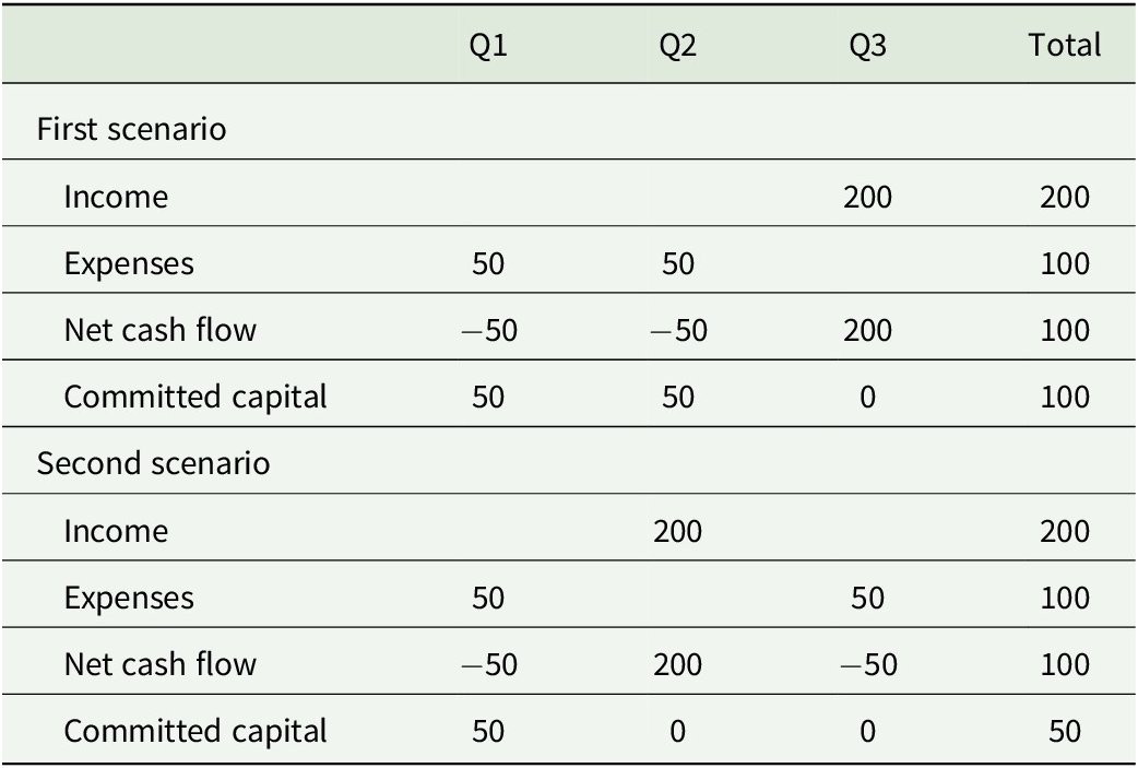
A simple example helps illustrate this concept. Suppose a farmer plans, over the course of a year, to spend $100 on inputs and receive $200 in income. Consider two alternative scenarios in which total costs and cash inflows are identical, but the timing of those inflows and outflows differs. The timing of these cash flows affects the farmer’s financial position. In the first scenario, the farmer must incur input expenses before receiving any income. Specifically, the farmer spends $50, then another $50, and only afterward begins to receive income. In this case, cash flow becomes negative by up to $100 before any income is received. As a result, the full $100 must be financed upfront, implying that all capital expenditure is also committed capital. In the second scenario, the timing of income allows for partial self-financing. The farmer first spends $50, then receives a payment of $200, and only afterward incurs the remaining $50 in costs. In this case, the maximum cash deficit is only $50, since the second round of expenses can be financed using the income already generated. Consequently, only $50 constitutes committed capital (Table 1).
Example of cash flow dynamics and committed capital

Table 1. Long description
The table is organized into five columns: Category, Q 1, Q 2, Q 3, and Total. It is divided into two main sections.
First scenario:
* Income: 200 in Q 3; Total 200.
* Expenses: 50 in Q 1; 50 in Q 2; Total 100.
* Net cash flow: minus 50 in Q 1; minus 50 in Q 2; 200 in Q 3; Total 100.
* Committed capital: 50 in Q 1; 50 in Q 2; 0 in Q 3; Total 100.
Second scenario:
* Income: 200 in Q 2; Total 200.
* Expenses: 50 in Q 1; 50 in Q 3; Total 100.
* Net cash flow: minus 50 in Q 1; 200 in Q 2; minus 50 in Q 3.
* Committed capital: 50 in Q 1; 0 in Q 2; 0 in Q 3; Total 50.
Note: The table compares two cash flow structures with identical aggregate costs and revenues. Differences in the sequencing of expenditures and revenues lead to distinct peak financing requirements.
Both scenarios have identical income and expense values. However, the amount of capital that must be committed differs substantially: 100 in the first scenario versus 50 in the second. This example shows that economic performance depends not only on aggregate costs and revenues, but also on the timing and sequencing of cash flows.
This becomes particularly relevant when considering farmers’ seasonal financing needs (such as purchasing seeds and fertilizers at the beginning of the season) and exposure to risks (such as weather or price variability), along with their access to credit. As Khan et al. (Reference Khan, Nouman, Negrut, Abban, Cismas and Siddiqi2024) note, these features differ from the standard repayment schedules of traditional loans, leading farmers to face what they define as supply constraints.
The second indicator is Turnover Velocity, defined as the ratio of expended capital to committed capital. It represents the frequency at which committed capital returns into the activity as reinvested earnings; i.e., the intensity with which committed capital is recovered and reinvested within the analyzed period (Romero and Benchimol, Reference Romero and Benchimol2008). Rather than constituting a conventional accounting turnover ratio, it reflects the circulation of capital that was effectively required to cover financing gaps within the analyzed period. It indicates the extent to which the valorization process of committed capital can finance capital expenditures, or in other words, the proportion of expended capital that is covered by the income generated through the valorization process of committed capital.
Finally, the Profit Rate is generally used as an indicator of the enterprise’s capacity to accumulate economic resources over time, as it expresses the relationship between net returns and the capital in production. Within the SIG framework, however, this ratio is conceptually redefined: the denominator is not the initial investment, but committed capital. Accordingly, the profit rate is measured as the ratio between net clash flow (NCF) and committed capital during the analyzed period. By relating net returns to the net capital effectively tied up in the production process (committed capital), the indicator captures the intensity with which the system valorizes the capital that must actually be financed within the analyzed period.
It is essential to distinguish between initial investment and committed capital. The initial investment refers to the stock of resources allocated at the outset of the project, typically fixed assets, infrastructure, or expenditures required to initiate operations. It is a point-in-time magnitude. Committed capital, by contrast, is a flow-based and structurally determined magnitude. It emerges endogenously from the interaction between cost structure, production timing, and revenue realization. While the initial investment may remain constant, committed capital can vary across periods depending on the system’s financial structure.
The profit rate defined in this way also differs from other measurement criteria such as net present value. NPV is an inter-temporal valuation tool that depends on an exogenously determined discount rate reflecting the opportunity cost of capital. It measures the net monetary surplus generated by a project after discounting future cash flows. While widely regarded as a consistent investment appraisal criterion, NPV does not constitute a profitability ratio in a strict sense, since it produces an absolute monetary value. Moreover, its result is highly sensitive to the selected discount rate, an estimate that, particularly in small-scale agricultural contexts, may involve substantial uncertainty regarding opportunity costs, risk premiums, and financing conditions. Although NPV can incorporate working capital requirements and temporary liquidity deficits, its analytical focus remains centered on inter-temporal valuation. In contrast, the SIGCHA framework shifts the analytical lens toward the endogenous configuration of capital flows within the production cycle. The profit rate, as defined, measures capital valorization as an emergent property of the system’s temporal and financial structure, rather than as a result derived from externally imposed discount assumptions.
Data collection
To explore the economic benefits of crop diversification and CSA systems on small-scale horticultural activity, we simulated three different farm management scenarios and compared their outcomes. These scenarios were constructed using detailed production and marketing data from three horticultural farms located in the Andean valley region Comarca Andina del Paralelo 42 (CAP42), in Northern Patagonia, Argentina. The study region is characterized by its cold temperate climate conditions, with an average annual temperature of 9.8°C, and substantial levels of rainfall, averaging around 900 mm per year. The region’s relative altitude and the orientation of its valleys, together with its fertile soils, create favorable climatic conditions conducive to agricultural and livestock activities (IICA, 2013). Weather conditions allow for year-round production with a high seasonality. The horticultural production season typically starts in June, peaks from December to March and gradually declines in April/May.
Data were collected as part of a PAR process in which a co-inquiry on economic farm management was conducted with a group of horticultural farmers (Frank et al., Reference Frank, Amoroso, Propedo and Kaufmann2022). Beyond exploring the unique specifics of each case, this type of research supports conceptual development and contributes to the building of broader theories related to social structures and processes (Eisenhardt, Reference Eisenhardt1989). This democratic and emancipatory perspective is deeply rooted in the theory of co-inquiry, wherein individuals possess the right to participate in research and influence the significance of the results about their own experiences, as well as to express their values in the research design. The methodological and conceptual findings from the conducted co-inquiry are reported elsewhere (Frank et al., Reference Frank, Amoroso, Propedo and Kaufmann2022).
The three farms involved in data collection were engaged in a joint management scheme covering 3 ha of intensive organic vegetable production for self-consumption and local marketing. Although these farms constituted distinct management units, they coordinated input procurement and product marketing. Over 30 vegetable species were cultivated in both greenhouses and irrigated fields, employing small-scale mechanization for soil preparation and seeding, while other cropping tasks were carried out manually.
One of the main challenges in obtaining economic evidence on diversified horticulture production lies in the lack of a farm data recording culture among farmers, and the lack of adequate tools for data systematization (Basir et al., Reference Basir, Buckmaster, Raturi and Zhang2024). After a review of partially existing farm data and methods recommended by the literature, it was decided to conduct a joint data collection process between researchers and farmers over two consecutive years, organized in two main stages. During the first stage (2019–2020), the work focused on collecting information on crop technical characteristics (such as sowing methods and yields), as well as economic and financial data. A total of 10 group sessions were held between the research team and six farmers from the participating farming projects to define data collection parameters and ensure methodological consistency across sites. During the second stage (2020–2021), the focus shifted to organizing, processing, and analyzing the information obtained during the previous season, with particular attention to economic and financial aspects, including the valuation of fixed capital and current accounts (i.e., cash inflows and outflows). In addition to the group sessions, in total, more than 20 individual meetings were conducted between researchers and farmers.
Base economic scenarios
The SIGCHA software models both technical and financial variables that influence farm activity, dynamically constructs the corresponding capital chronostructure, and calculates the associated indicators. It also allows the simulation of alternative scenarios by introducing variations in managerial decisions (e.g., crop rotations, planting dates, irrigation practices, machinery use, or varietal selection) and financial conditions (e.g., input prices, labor costs, interest rates, or output prices). Starting from a ‘base chronostructure’, these variations make it possible to construct counterfactual ‘what-if’ scenarios, such as the impact of a pest affecting a specific crop or a change in marketing strategy, and to quantify their effects on capital dynamics through changes in profit rate, committed capital, and turnover rate, thereby enabling systematic ex ante assessment of their economic implications (Levín and Kicillof, Reference Levín and Kicillof1999; Propedo, Reference Propedo, Intriago Barreno, Llerena Hidalgo and Intriago Barreno2019).
In this study, the simulation exercise is structured as an ex ante planning problem situated at the onset of the production cycle, where farmers allocate given endowments of fixed capital and labor under resource constraints. Within this decision framework, alternative crop portfolios and production scales are modeled and compared, contrasting higher versus lower levels of diversification to assess their relative effects on economic performance and capital dynamics.
To this end, three Base Economic Scenarios (BES) were developed: BES1 representing a highly diversified cropping system, BES2 a moderately diversified system, and BES3 a low-diversification system. The analysis is based on 1 ha of land, managed through crop rotation and intercropping practices (Figure 1). Production is organized in beds measuring 50 m in length and 1 m in width, consistent with the techniques and technologies used by the farms included in the study. The three scenarios were designed as ceteris paribus comparisons: technical conditions, farm area, and labor use were held constant across BES1, BES2, and BES3 to isolate the effect of crop portfolio composition on financial performance. The central analytical question is: holding technical conditions constant, which crop portfolio composition yields the most favorable financial performance?
Crops across base economic scenarios. Spatial distribution of crops under the three Base Economic Scenarios across 1 ha. Panel A (BES1) represents a highly diversified agroecological system based on a reference farm, comprising 35 crops. Panel B (BES2) represents a moderately diversified system comprising six crops, selected for profitability and co-designed with farmers. Panel C (BES3) represents a low-diversity system comprising three crops reflecting conventional horticultural production practices in the study region.

Figure 1. Long description
A three-panel illustration of circular farm plots labeled 1 Hectare.
* Panel A, Base Economic Scenario 1 High diversity, shows a circular plot divided into approximately 35 irregular, multi-colored polygonal segments. Each segment contains a different crop icon, including leafy greens, root vegetables like carrots and radishes, fruiting plants like tomatoes and eggplants, grains, and flowers, representing a complex agroecological system.
* Panel B, Base Economic Scenario 2 Moderate diversity, shows a circular plot divided into six equal wedge-shaped sectors. Clockwise from the top-left, the sectors contain: 12 carrots, 5 large pumpkins, 6 heads of cabbage, 5 small green squashes with radishes and bok choy, 12 more carrots, and 5 heads of bok choy.
* Panel C, Base Economic Scenario 3 Low diversity, shows a circular plot divided into three large unequal sectors. The largest sector on the right contains 24 onions. The bottom sector contains 12 heads of cabbage. The left sector contains 18 carrots. This represents a conventional horticultural production practice.
Following the structure and operational logic of the SIGCHA framework, a set of variables was defined to construct the chronostructures of BES1, BES2, and BES3:
1. Technical information on crops: key agronomic parameters defining the management and performance of each crop (Appendix). These include the sowing date and method (direct seeding or transplanting), spacing between plants and rows (cm), the number of days until the first harvest, the expected yield per square meter (kg), the number of successive crops per planting (for instance, how many times lettuce is sown within a season, as several crops complete more than one sowing–harvest cycle per season and are managed through sequential sowing sections to ensure a continuous harvest), and the interval between harvests (as in the case of chard or kale, which are sown once but harvested multiple times during the season). Technical information on crops was collected through participatory sessions between researchers and farmers between 2019 and 2020.
To assess yields, a field trial was planned and conducted to estimate the productivity of 12 different crops (kg per square meter). Crops were selected based on their relevance to farmers, considering both sales volume and cultivated area. For each crop, two linear meters of rows were randomly marked in two to three different patches after sowing or transplanting, to ensure randomization and allow for controlled harvesting and weighing. The corresponding area was converted into square meters to standardize yield estimates. Due to the diversity of crops, different methods were applied for recording harvested quantities, depending on each crop’s harvesting characteristics. For single-harvest crops, such as pumpkin or lettuce, the harvested quantities (in kilograms) were directly recorded for each sample. For continuous-harvest crops, where plants produce throughout the season, yields were recorded weekly over the entire production cycle. At the end of the season, the total kilograms harvested per crop were associated with the corresponding cultivated area. To calculate the cultivated area, the cropping calendar used by farmers, which included the number of sowings, the area, and the location of each crop, was cross-checked with field data on plot size and the square meters allocated to each crop.
For crops not included in the field trial, data collection relied on production planning records maintained by farmers, primarily spreadsheets and similar documents. Given time and resource constraints, missing information was supplemented using farmers’ experience and estimates. Since this knowledge had not been previously systematized, standardized Excel templates were created to organize and consolidate all available data. This process involved not only the systematization of yield data but also of all other information relevant for the subsequent economic calculations.
2. Sowing/transplanting and harvesting calendars: The crop calendar specifies the spatial distribution and quantities of each crop, along with their corresponding sowing and harvesting dates. BES1 was based on the crop calendar of one of the farms participating in this study, considered an agroecological reference model in the region. It includes 35 different crops cultivated on one hectare using crop rotation and intercropping practices. In defining BES2, we asked: given one hectare of land, which crop combination would maximize profitability? To address this question, we consulted all participating farmers to identify the crops they considered most profitable and reached consensus on a reduced set of crops: squash, carrot, zucchini, lettuce, chard, and cabbage. For BES3, we consulted a technical advisor from the Rural Change Program (Cambio Rural) of the National Institute of Agricultural Technology (INTA), who works closely with horticultural farmers in the region. Based on this consultation, we identified the crops most commonly cultivated in low-diversification horticultural systems, which are generally managed under conventional production practices. The resulting scenario included lettuce, onion, and carrot. In BES2 and BES3, the area allocated to each crop and the corresponding sowing schedules were co-designed with farmers and technical advisors, taking into account both technical constraints—such as the limited planting windows imposed by the cold climate—and market considerations. The resulting scenarios were designed to avoid both temporary overproduction of individual crops and periods without marketable produce, thereby reflecting farmers’ strategies for risk management and market coordination.
3. Labor expenses: In all scenarios, total labor use, and, therefore, labor costs, were held constant to isolate the effect of diversification strategies, given a fixed land area and labor capacity. This design choice reflects the model’s analytical objective: to identify which diversification strategy yields the most favorable capital structure and rate of return, given an equivalent endowment of resources, including labor use. The sensitivity of results to alternative labor use assumptions is examined separately in ‘Sensitivity analysis: Alternative labor assumptions’ section. Using detailed records of hours worked on the model farm, we estimated the labor requirements for a one-hectare horticultural system and calculated a monthly labor cost of $2,100, based on total hours worked during the 2019–2020 season, annualized over 12 months and valued at legal hourly wage rates in Argentina for 2020–2021.
4. Direct seed costs: Based on each crop’s technical parameters defined in ‘1’ and the crop calendar defined in ‘2’, SIGCHA computes the exact quantity of seeds required in the production season. All seeds were assumed to be purchased together on June 1, ensuring uninterrupted supply throughout the season.
5. Indirect costs: To project the remaining expenses, we analyzed the model farm’s income and expenditure records for the 2020–2021 season. Expenses were classified into the following categories: infrastructure rental, land rental, fuel, contracted machinery services, electricity and gas, administrative expenses, marketing expenses, infrastructure maintenance and repairs, machinery maintenance and repairs, agricultural inputs (excluding seeds, e.g., compost and fertilizers), and transportation. It is important to clarify that major investments in long-term assets (such as machinery) were excluded from the analysis. This decision is based upon the short-term scope of this analysis (1 year) and the presumption of the relative productive maturity of the enterprises, where major investments in fixed capital have been previously made. (Indirect cost: those costs that remain constant regardless of the production decision taken in terms of activities to be carried out and production levels. In a short-term analysis, they are generally represented by structural costs, amortization and interest on improvements, machinery and general expenses. Structural costs include expenses arising from administration, taxes and the structure of the farm as a productive unit and not related to any specific activity.)
6. Sales prices: The price matrix utilized was the price matrix established by the model farm for the 2020–2021 season.
SIGCHA estimates income by combining variables included in groups 1–3. Once the crop calendar and the yield per mt2 of each crop have been established, we used the SIGCHA model to compute the quantities of products available for sale throughout the season. By linking this with the price matrix, the total income for each crop is estimated. Similarly, temporary outflows (e.g., inputs, wages) are estimated based on variables encompassed in groups 3, 4, 5, and 6. In this way, the capital chronostructure is constructed, and the model’s dependent variables are calculated.
Results
Simulation 1: Financial performance across diversification levels
The chronostructures of three crop portfolio scenarios were constructed and compared (Table 2). BES3—comprising lettuce, onion, and carrot, representative of conventional horticultural production in the region—generates the lowest profit rate (239%) and the lowest net cash flow ($41,561). BES2, a moderately diversified system of six crops selected for profitability, generates a net cash flow of $62,564 and a profit rate of 347%. BES1, a highly diversified agroecological system of 35 crops, generates a net cash flow of $60,577—marginally below BES2—yet achieves the highest profit rate of 409%. Together, the three scenarios establish a clear profit-diversification gradient: BES3 (239%) → BES2 (347%) → BES1 (409%).
Economic indicators across simulated scenarios

Table 2. Long description
The table consists of six columns representing different scenarios under the heading Chronostructure: B E S 1, B E S 2, B E S 3, B E S 1 C S A 1, B E S 1 loan, and B E S 1 C S A 2.
* Profit rate (percent): B E S 1 is 409; B E S 2 is 347; B E S 3 is 239; B E S 1 C S A 1 is 519; B E S 1 loan is 519; B E S 1 C S A 2 is 483.
* Committed capital: B E S 1 is $14,808; B E S 2 is $18,032; B E S 3 is $17,362; B E S 1 C S A 1 is $11,308; B E S 1 loan is $11,306; B E S 1 C S A 2 is $11,308.
* Turnover rate: B E S 1 is 2.29; B E S 2 is 1.92; B E S 3 is 1.96; B E S 1 C S A 1 is 3.00; B E S 1 loan is 3.83; B E S 1 C S A 2 is 3.00.
* Income: B E S 1 is $94,472; B E S 2 is $97,239; B E S 3 is $75,537; B E S 1 C S A 1 is $92,582; B E S 1 loan is $102,030; B E S 1 C S A 2 is $88,539.
* Expenses: B E S 1 is $33,894; B E S 2 is $34,675; B E S 3 is $33,975; B E S 1 C S A 1 is $33,894; B E S 1 loan is $43,298; B E S 1 C S A 2 is $33,894.
* Net cash flow: B E S 1 is $60,577; B E S 2 is $62,564; B E S 3 is $41,561; B E S 1 C S A 1 is $58,688; B E S 1 loan is $58,732; B E S 1 C S A 2 is $54,644.
Note: This table reports key economic indicators for different production and financing scenarios, including BES1 (high diversity), BES2 (moderate diversity), and alternative financial arrangements applied to BES1 (CSA and loan schemes). Indicators include profit rate (calculated using the SIGCHA methodology as the ratio of net cash flow to committed capital), committed capital, turnover rate, total income, total expenses, and net cash flow. The comparison highlights how both production diversity and financial structures influence profitability and capital requirements.
The discrepancy between net cash flow and profit rate in BES1 and BES2 is analytically significant. Assessed by NCF alone, BES2 appears slightly more profitable ($62,564 vs. $60,577), generating an apparent disincentive to diversify. However, when the temporal dimension is incorporated through SIGCHA, this conclusion reverses: BES1’s profit rate exceeds BES2’s by 62 percentage points, explained by its lower committed capital ($14,808 vs. $18,032). BES2, though composed of individually profitable crops, concentrates long-cycle crops that require sustained expenditure without generating income until late in the season, increasing the need for external financing. In BES3, even the NCF metric suggests that less diversification is disadvantageous: the narrower crop portfolio generates substantially lower total income, and the profit rate—at 239%—is the lowest across all scenarios. Notably, BES3’s committed capital ($17,362) is marginally lower than BES2’s ($18,032), reflecting the presence of lettuce, a short-cycle crop that generates early-season income and partially offsets financing needs. Yet this modest reduction does not compensate for the substantial income loss associated with minimal crop diversity.
While the NCF provides a static measure of profitability at the end of the production cycle, it fails to capture the timing of cash inflows and outflows. In contrast, SIGCHA integrates the temporal dimension of financial processes by quantifying committed capital, revealing when production requires external financing and when it becomes self-sustaining through its own revenues. By introducing this dynamic dimension, SIGCHA conceptualizes crops as a portfolio of projects in different stages of maturity: the capital portions associated with each crop have different turnover rates, yet are interconnected through the returns that become available for new investments as each cycle completes. By accounting for overlapping and simultaneous turnover cycles, the framework captures the economic-financial effects of crop portfolio composition, effects that aggregate end-of-cycle metrics systematically obscure.
These results point to a central insight: the financial advantages of diversification are not a direct function of the number of crops grown, but of the temporal composition of the portfolio and the cash flow dynamics it generates. What sets BES1 apart is not simply the breadth of its crop portfolio, but the strategic interaction between short-cycle and long-cycle crops. Staggered cash flows progressively compensate for financing needs throughout the production season, reducing committed capital and increasing capital efficiency. BES3 illustrates the opposite: even when a short-cycle crop (lettuce) partially reduces the financial burden, the insufficient breadth of the portfolio limits total revenue and undermines overall financial performance. This has a direct practical implication: financial planning of diversified systems must account not only for which crops are grown, but for when the capital they mobilize enters and exits the production cycle.
Simulation 2: Comparing CSA scheme and loan as mechanisms for farm financing
To compare alternative financing options for annual production in diversified systems, we simulated different scenarios for BES1. We compare a simulation of a CSA program to a scenario involving the adoption of a bank loan. The CSA design aimed to ensure straightforward and feasible implementation for farmers. Recognizing that a full-scale transition would be challenging to achieve immediately, the program was conceived as a pilot phase, an initial step toward gradual adoption. Specifically, it was framed as part of a mixed marketing strategy, whereby a portion of total output would be commercialized through the CSA while the remainder continued through existing sales channels. This approach enables a progressive integration of the CSA model without disrupting ongoing production and marketing operations. The simulation represents a potential strategy considered by farmers: ‘What would happen if we sold 10% of our production in advance to improve cash flow at the beginning of the season?’
The design also sought to minimize implementation costs, particularly those associated with production and distribution. In practice, the CSA does not entail an increase in production but rather a reallocation of existing outputs, with a share of the produce allocated to the CSA instead of traditional outlets such as farmers’ markets. As a result, the model assumes that no additional production infrastructure is required and that additional logistics and transportation costs are minimized. Similarly, member recruitment was expected to leverage existing communication tools, as most farms already use social media platforms (e.g., Instagram, Facebook, WhatsApp) for regular sales promotion, implying no additional labor or resource requirements.
In the study region, some CSAs are designed to include a price discount in favor of consumers as an incentive for participation. To analyze the impact of such a system on profitability, we designed a CSA scheme for BES1 with the following characteristics:
-
1. Ten percent of the total estimated harvest, equivalent to 10% of total income ($94,472), is offered for pre-sale under the CSA scheme.
-
2. CSA consumers receive a 20% discount exclusively for advance purchases.
-
3. Pre-sale income is received at the beginning of September, coinciding with the start of the growing season.
-
4. The remaining 90% of production continues to be sold as originally planned, primarily through weekly sales at local farmers’ markets.
-
5. At this stage, the CSA is not yet designed at the operational level, i.e., we have not calculated how many individual CSA shares or subscriptions correspond to this 10% of production. Instead, the analysis focuses on the financial implications of reallocating a portion of the harvest, allowing us to explore the potential effects on cash flow, capital commitment, and profitability before scaling up to a fully operational CSA program.
Given these characteristics, this simulation implies an anticipated income of $7,557 (see the fourth column in Table 2), which corresponds to 10% of the total estimated income for the season in BES1 ($94,472), with a 20% discount on prices. Compared to BES1, the pre-sale strategy (allocating 10% of the total estimated production to CSAs) reduces the NCF from $60,577 to $58,688 due to the 20% price discount for CSA consumers. However, it decreases committed capital by 24% from $14,808 to $11,308. This reduction arises because the income received at the beginning of the season offsets expenses that would otherwise represent committed capital. In other words, although total revenues generated through the CSA scheme are lower than those obtained through conventional marketing channels (since the CSA design includes a price reduction to attract consumers), these early payments reduce the need to finance operating expenses through savings or credit. Consequently, it boosts the profit rate of the chronostructure, rising from 409% to 519%.
Within the framework of analyzing financing alternatives for diversified farming systems, following the evaluation of the 10% pre-sale strategy through a CSA scheme, a second approach based on access to bank credit was explored. This exercise enables a comparison between two alternative financial management mechanisms: one based on direct relationships with consumers and the other relying on the credit system. The objective was to determine what credit structure (in terms of loan term, interest rate, and repayment schedule) would be required for a loan equivalent to the amount received through the CSA pre-sale ($7,557) to yield comparable financial results (similar and committed capital).
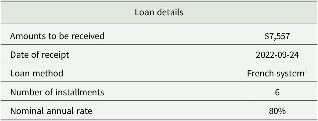
After simulating various alternatives, the loan with the conditions summarized in Table 3 was identified as the closest equivalent for the farmer (see fifth column in Table 2). When comparing the final results of the CSA pre-sale and the bank loan, the latter proves to be a more costly option. Although both scenarios result in the same level of committed capital, the loan increases total expenditures by $9,404 (from $33,894 to $43,298) due to interest payments. In other words, the financial cost of credit, represented by interest charges, is higher than the implicit cost of the CSA strategy, which stems from the price reduction offered to attract consumers (amounting to $1,889, corresponding to a 20% discount on 10% of total production). Thus, consumer-based financing mechanisms may represent a more sustainable strategy for diversified farming systems.
Loan characteristics comparable to CSA

Table 3. Long description
The table consists of a header row and five data rows.
Header: Loan details (spanning both columns).
Row 1: Amounts to be received is $7,557.
Row 2: Date of receipt is 2022-09-24.
Row 3: Loan method is French system super 1.
Row 4: Number of installments is 6.
Row 5: Nominal annual rate is 80%.
A footnote for super 1 explains that under the French amortization system, borrowers make equal periodic payments where the interest portion declines and the principal portion increases over time.
1 Under the French amortization system, borrowers make equal periodic payments over the loan term. Each payment includes both principal and interest, with the interest portion declining and the principal portion increasing over time.
Note: The table reports the parameters of a loan instrument constructed to mimic the intertemporal cash flow structure of a CSA, including disbursement, repayment schedule (French system), and nominal interest rate.
We also explored alternative financing configurations for CSA programs to assess which options are most feasible and beneficial for farmers. To this end, a new scenario was simulated to evaluate the financial implications of modifying the CSA conditions. In this case, instead of pre-selling 10% of the yield with a 20% discount, 20% of the yield was assumed to be pre-sold with a 30% discount for consumers who pay in advance. Using SIGCHA, this alternative was modeled and compared with the previous scenario (CSA1 in BES1).
The results show that the profit rate decreases to 483% (see sixth column in Table 2), as the reduction in committed capital (resulting from the income received earlier in the season) does not offset the decrease in total income (caused by the reduction price of 30%). This exercise illustrates the importance of carefully designing financial strategies within CSA schemes to balance liquidity improvements with potential income trade-offs, underscoring the need to continue developing information and management tools that support more resilient and sustainable farm economies.
Sensitivity analysis: Alternative labor assumptions
Labor requirements are likely to vary depending on diversification strategies. Several factors could account for such differences: managing a larger number of crops simultaneously may increase total labor input; planning, logistics, and coordination demands tend to grow with the complexity of the crop portfolio. However, in the context of this study, data on crop-specific labor requirements for the range of species and management practices represented in BES1 and BES2 are not available, which prevents the parameterization of differentiated labor scenarios. Furthermore, the available evidence in the broader literature does not provide consistent guidance regarding these differences. Some studies suggest that agroecological and diversified systems entail higher labor demands, especially during transition periods, while other studies find no systematic increase in already established systems, and simulation results indicate that labor requirements depend more on system design than on the level of diversity itself (Morel, San Cristobal and Léger, Reference Morel, San Cristobal and Léger2017; Stratton, Wittman and Blesh, Reference Stratton, Wittman and Blesh2021). The uncertainty surrounding this assumption is therefore examined through two complementary sensitivity analyses.
First, a sensitivity analysis was conducted on BES2 (moderate diversity—6 crops) by reducing the labor endowment by one and two workers while holding all other parameters constant. With one fewer worker, BES2’s profit rate (408%) converges to BES1’s baseline (409%), and with two fewer workers it exceeds it (483%). This finding is analytically relevant: it demonstrates that the ceteris paribus assumption does not structurally advantage BES1. Furthermore, BES1’s advantage is not primarily expressed through profit rate but through committed capital: even when BES2 is assumed to operate with two fewer workers, committed capital ($14,432) remains close to BES1’s baseline ($14,808). The structural contribution of diversification to reducing the financing burden is therefore preserved across all labor scenarios examined. These scenarios assume constant output levels regardless of the labor reduction—implying either surplus labor in the baseline or increased workload for remaining workers without additional compensation. The financial gains reported therefore represent an upper bound, which makes BES1’s committed capital advantage a conservative result. It should be noted, however, that the scenarios assuming one and two fewer workers imply the elimination of one and two permanent farm jobs, respectively. Improved profit rate under reduced labor is therefore achieved at a direct cost to rural employment—a trade-off that falls outside the boundaries of the financial model but carries significant implications for rural employment and livelihood.
A second analysis examined the effect of adapting worker allocation to the farm’s seasonal rhythm rather than remaining constant year-round. In this cyclical scenario, the number of workers ranges from 4 during the low-production months to 7 at peak season, reflecting seasonal staffing patterns documented among producers in the study region. Under this configuration, the profit rate rises substantially for both systems—BES1 reaches 572% and BES2 reaches 465%—while committed capital falls to $10,908 and $13,832 respectively, reflecting a reduced financing burden when labor costs adjust to match seasonal production intensity.
When one worker is removed from the cyclical BES2 variant, its profit rate (575%) marginally surpasses BES1’s (572%). As in the static sensitivity analysis, however, this near-convergence in profit rates does not undermine the case for diversification: BES1’s committed capital ($10,908) remains $1,124 lower than that of the reduced-labor cyclical BES2 scenario ($12,032), meaning that the financing burden is structurally lower in the more diversified system regardless of labor assumptions. The cyclical analysis instead highlights that adaptive labor management amplifies the financial returns of any production system, and that this effect is fully compatible with the benefits of crop diversification.
Discussion
Conventional, low-diversity agricultural models have led to various ecological, social, and economic issues, including biodiversity loss and adverse effects on small-scale farmers. Transitions toward sustainable agriculture require both ecological and social innovation and economic viability. While the ecological innovations have been extensively studied, less attention has been paid to the financial implications of adopting agroecological practices (Rasmussen et al., Reference Rasmussen, Grass, Mehrabi, Smith, Bezner-Kerr, Blesh, Garibaldi, Isaac, Kennedy, Wittman, Batáry, Buchori, Cerda, Chará, Crowder, Darras, DeMaster, Garcia and Gómez2024). However, economic considerations are crucial for the widespread adoption of sustainable practices (Ansari and Tabassum, Reference Ansari and Tabassum2018; Feliciano, Reference Feliciano2022). In this study, we focus on the adoption of crop diversification and CSA marketing practices in small-scale horticultural systems in Northern Patagonia, Argentina.
The results of Simulation 1 demonstrate that diversification can improve the economic performance of horticulture by generating more complex and temporally distributed cash flows. In highly diversified systems such as BES1, the combination of crops with different production cycles produces earlier income streams and lowers the reliance on external financing, resulting in a higher profit rate despite comparable overall net cash flows between BES1 and BES2. This pattern suggests that the economic advantages of crop diversification arise not merely from increased output, but from the structural dynamics of capital circulation it induces. Capturing these dynamics requires analytical tools capable of representing temporal variability and interdependencies among production components, such as the SIGCHA model.
These findings align with previous empirical research showing that diversified farms tend to experience lower income volatility and greater resilience to climatic and market shocks, even when their end-of-cycle profits are comparable to or slightly below those of specialized farms (Harkness et al., Reference Harkness, Areal, Semenov, Senapati, Shield and Bishop2021; Sánchez et al., Reference Sánchez, Kamau, Grazioli and Jones2022). Our results further suggest that diversification enhances cash-flow stability and reduces seasonal liquidity constraints by staggering income across different crops and over time. Likewise, studies on cash-crop systems with low levels of crop diversification highlight that long-cycle crops can generate delayed revenues and periods of liquidity stress (Anderman et al., Reference Anderman, Remans, Wood, DeRosa and DeFries2014; Melkani et al., Reference Melkani, Mason, Mather, Chisanga and Jayne2025). This is consistent with our finding that BES2, dominated by long-cycle crops, requires greater capital exposure during the production season. Therefore, our results reinforce the argument that diversification not only affects ecological or productive stability but also shapes the temporal structure of cash flows and financial resilience.
Nevertheless, while diversification influences internal cash-flow dynamics, external financing mechanisms also play a crucial role in determining overall liquidity stability. To explore this dimension, Simulation 2 examines the role of financing mechanisms. While CSA schemes have been associated with strengthened farmer–consumer relationships and increased resilience of local food systems (Galt, Reference Galt2013; Furness et al., Reference Furness, Sanderson Bellamy, Clear, Mitchell Finnigan, Meador, Mills, Milne and Sharp2022), our results suggest that they also provide not only social but also economic and financial benefits for farmers. The CSA scenario simulated for BES1 highlights the potential of consumer-based financing, such as the pre-selling concept, as a viable alternative to credit-based mechanisms. Although total income decreased due to the price discount offered to consumers, the scenario simultaneously reduced committed capital and improved the profit rate by more than 100 percentage points compared to the baseline. This result underscores the role of CSA schemes in mitigating early-cycle liquidity constraints. In contrast, the loan-based scenario (BES1 Loan) showed that interest payments substantially increase total expenditures. These findings are consistent with broader evidence showing that conventional loans often exacerbate liquidity stress when repayment schedules do not align with the dynamics of agricultural cash flows (Khan et al., Reference Khan, Nouman, Negrut, Abban, Cismas and Siddiqi2024). Therefore, the comparative analysis suggests that consumer-based financing may represent a more sustainable alternative for diversified systems, offering liquidity support without the burden of debt.
These liquidity benefits extend beyond farm-level capital dynamics to the income of farmer households. The committed capital metric provides a quantitative basis for understanding when the farm’s financing burden peaks and by how much—and this timing has direct implications for household cash availability. Producers in the study region fall into two broad profiles: those who depend exclusively on farm income, and those who supplement it with part-time off-farm employment during the low-production season. For both groups, the CSA pre-payment mechanism provides a concrete household benefit: by advancing revenues to the beginning of the production cycle, it makes cash available to pay labor—including the farmers themselves—precisely during the months when farm sales are lowest. Rather than merely offering an alternative source of financing, CSA pre-payments directly improve household liquidity at the moment when it is most constrained.
These findings must, however, be read alongside broader evidence documenting the economic challenges of CSA. Studies in other global contexts consistently show that CSA farmers struggle to earn adequate livelihoods, with farm incomes frequently falling below median wage levels (Paul, Reference Paul2019), and that the social obligations inherent to the CSA model can generate self-exploitation dynamics that erode the financial benefits of pre-financing arrangements (Galt, Reference Galt2013). These considerations reinforce the relevance of the second CSA scenario (BES1 CSA2) analyzed in this study: when discount rates in the pre-selling scheme are set too high or the pre-sold proportion exceeds an optimal threshold, liquidity benefits are outweighed by income losses. Evidence-based calibration of CSA design parameters is therefore not merely a matter of financial optimization but a safeguard against the self-exploitation dynamics documented in the empirical literature.
Beyond the design of the financing mechanisms, the robustness of the baseline results under alternative labor assumptions deserves attention. As detailed in ‘Sensitivity analysis: Alternative labor assumptions’ section, two complementary sensitivity analyses were conducted, given that crop-specific labor benchmarks for the diversification levels represented are unavailable for this context and the direction of any differential labor demand remains uncertain in the literature. The results reveal a trade-off between financial optimization and rural employment generation. Reducing the labor endowment in BES2 improves its profit rate—matching that of BES1 with one fewer worker and exceeding it with two fewer workers—but does so at the cost of eliminating permanent farm jobs. This highlights an employment dimension that aggregate profitability indicators do not capture: a highly diversified system can sustain higher levels of employment while maintaining greater capital efficiency.
The cyclical labor allocation analysis complements these findings. Allowing labor allocation to adapt to the farm’s seasonal requirements substantially improves the financial performance of both systems, increasing the profit rate to 572% in BES1 and 465% in BES2 while reducing committed capital accordingly. Even when one worker is removed from the cyclical BES2 scenario, BES1 retains its structural advantage in terms of committed capital. These findings suggest that adaptive labor management can improve financial performance across different production systems, while crop diversification continues to provide structural advantages in capital efficiency. In contexts of rural outmigration and precarious agricultural labor markets, the capacity of a farming system to generate stable employment constitutes an important dimension of economic sustainability that is not fully reflected in conventional profitability metrics.
Conclusions
This study examined the economic outcomes of adopting crop diversification and CSA in small-scale horticultural systems in Northern Patagonia, Argentina. A central conceptual contribution is the treatment of crops as a portfolio of overlapping capital cycles: the returns generated by each crop become available for reinvestment, and the temporal sequencing of these cycles determines the overall financing need of the system. Across the three baseline scenarios analyzed—BES3 (3 crops; profit rate 239%), BES2 (6 crops; 347%), and BES1 (35 crops; 409%)—profit rates increase systematically with diversification level. This gradient, however, is not a direct function of the number of crops grown: BES3 exhibits a marginally lower committed capital than BES2 despite being less diverse, because its portfolio includes a short-cycle crop that generates early-season income. The decisive advantage of BES1 lies in the deliberate temporal composition of its portfolio, in which staggered cash inflows from crops with heterogeneous production cycles progressively offset financing needs throughout the season. These findings suggest that the financial benefits of diversification depend critically on how diversity is planned in relation to cash flow dynamics, rather than on diversification as such.
We also found that the CSA model represents a marketing approach that substantially shapes the capital chronostructure. By advancing consumer payments to the beginning of the production cycle, CSA directly reduces the committed capital that farmers must finance through savings or credit—a period that has traditionally been associated with significant financial pressure. In the baseline CSA scenario, committed capital fell by 24%, and the profit rate rose from 409% to 519%, despite a reduction in total income due to the price discount offered to members. A loan structured to replicate the same liquidity effect required $9,404 in additional expenditure due to interest charges, compared to an implicit cost of $1,889 under the CSA arrangement. A second CSA scenario demonstrated that more aggressive parameterization—pre-selling 20% of production at a 30% discount—erodes these gains, with the profit rate declining to 483%. These results confirm that consumer-based financing can function as a financially rational alternative to credit, particularly for farmers facing capitalization constraints, provided that design parameters are calibrated to balance liquidity benefits against income losses.
Sensitivity analyses confirm the robustness of the baseline findings under alternative labor assumptions. When the labor endowment of BES2 is reduced, its profit rate converges toward or exceeds that of BES1; however, BES1’s structural advantage in committed capital is preserved across all scenarios. This finding carries an important social dimension: improvements in financial performance through labor reduction imply the elimination of permanent farm jobs—a trade-off that aggregate financial metrics do not capture, but that is consequential in contexts of rural outmigration and precarious agricultural labor markets. A cyclical labor analysis further demonstrates that adaptive labor management amplifies financial returns across all scenarios, reinforcing that labor flexibility and crop diversification are complementary rather than substitutable strategies.
Together, these findings advance our understanding of the economic dimensions of the transition toward more sustainable agricultural systems and illustrate the value of dynamic capital chronostructure analysis as a planning tool for farmers, advisors, and policymakers. By making the temporal structure of cash flows visible and quantifiable, the SIGCHA framework enables evaluation of diversification and financing strategies not only by their aggregate outcomes but by the capital dynamics they generate throughout the production cycle. Future research should address several open questions: empirical measurement of labor requirements per crop type in diversified horticultural systems would allow more refined scenario parameterization; extension of the framework to other agroclimatic regions would test the generalizability of these results; and household-level analysis integrating on-farm and off-farm income streams would provide a more complete account of financial resilience for smallholder families.
Data availability statement
The data that support the findings of this study are available from the corresponding author upon reasonable request. Due to privacy and ethical considerations related to participating farmers, some restrictions apply.
Acknowledgments
We are especially grateful to the farmers who generously participated in this project. Their openness and collaboration were essential, and we hope the results of this study will be of practical benefit to them. During the preparation of this work, the authors used ChatGPT (OpenAI) and Claude (Anthropic) to improve the readability and language of the manuscript (e.g., English grammar). After using this tool, the authors reviewed and edited the content as needed and take full responsibility for the content of the published article.
Author contribution
M.P. and M.F. collected the data. M.P. and M.G. analyzed the data. M.P., M.F., and H.W. designed the methodology. M.P. wrote the original draft. All authors contributed to the interpretation of the results, revised the manuscript, and approved the final version.
Funding statement
This research did not receive any specific grant from funding agencies in the public, commercial, or not-for-profit sectors. The first author’s research was supported by a doctoral fellowship from the Consejo Nacional de Investigaciones Científicas y Técnicas (CONICET), Argentina, and an Emerging Leaders in the Americas Program (ELAP) scholarship, Canada, which provided financial support during the period in which the analyses were conducted and the manuscript was prepared.
Competing interests
The authors declare no conflicts of interest.
Appendix: Technical crop information
This appendix summarizes the key agronomic parameters used to characterize crop management and performance in the analyzed scenarios. The information was gathered collaboratively from farmers and researchers and systematized into standardized spreadsheets to support modeling and comparative analysis.
Technical crop information

Table A1. Long description
The table consists of 8 columns: Crop, Sowing, Yield per m super 2 (kg), Distance between plants (cm), Distance between rows (cm), Days until first harvest, Number of harvests per planting, and Days between harvests.
Key data points for selected crops include:
* Basil: Seedling, 1 kg yield, 30 cm plant distance, 40 cm row distance, 68 days to harvest, 13 harvests.
* Beet: Direct seed, 8 kg yield, 5 cm plant distance, 30 cm row distance, 90 days to harvest, 21 harvests.
* Carrot: Direct seed, 10 kg yield, 1 cm plant distance, 15 cm row distance, 120 days to harvest, 21 harvests.
* Garlic: Direct seed, 2 kg yield, 15 cm plant distance, 30 cm row distance, 240 days to harvest, 1 harvest.
* Kale: Seedling, 5 kg yield, 45 cm plant distance, 60 cm row distance, 60 days to harvest, 21 harvests.
* Squash: Direct seed, 7 kg yield, 100 cm plant distance, 110 cm row distance, 120 days to harvest, 16 harvests.
* Tomato: Seedling, 5 kg yield, 45 cm plant distance, 110 cm row distance, 120 days to harvest, 13 harvests.
All crops listed have a consistent 7 days between harvests.




 Open access

