1 Introduction
Flow around a bluff body is a common phenomenon in our daily life, occurring when wind blows past a tall building and a power line or water flows past a submarine and a bridge pier. When the Reynolds number exceeds a critical value, periodic vortex shedding appears in the wake, causing a significant drop of base pressure, structural vibrations, acoustic noise, enhanced mixing and increases in the mean drag and lift fluctuations (Choi, Jeon & Kim Reference Choi, Jeon and Kim2008). Complex flow phenomena, such as flow separation, shear layer instability and vortex shedding, appear when flow passes across a bluff body (Huang, Hsu & Chiu Reference Huang, Hsu and Chiu2014). Effective control methods must be used in engineering applications to reduce the negative impacts of vortex shedding.
As a typical blunt body, the square cylinder has attracted the interest of many researchers. For the circular cylinder, flow separates from its continuous surface, while for the square cylinder, the separation points are fixed on the front corners. Therefore, control methods by changing the boundary-layer characteristics to delay separation are inapplicable. Flow control of the square cylinder acts on the wake directly, changing the behaviours of vortex shedding (Choi et al.
Reference Choi, Jeon and Kim2008). For cases where a small rod was set upstream of the square cylinder to control the flow, Igarashi (Reference Igarashi1997) changed the diameter of the control rod and the spacing between the rod and the prism, and observed two flow modes. In mode A, there were vortices shedding from the rod. In mode B, however, vortices shedding from the rod disappeared and shear layers of the rod reattached on the upward surface of the square cylinder. The critical spacing where the modes changed was defined. When the spacing exceeded the critical value, the Strouhal number decreased, meanwhile, the drag of the square cylinder decreased by 50 %. At the spacing below the critical value, the Strouhal number increased, and approximately 70 % drag reduction was achieved. Zhang et al. (Reference Zhang, Wang, Lu and Mi2005) investigated the aerodynamic characteristics of the flow around a square cylinder with an upstream rod in a staggered arrangement by pressure measurement and the hydrogen bubble technique. For the rod and the square prism in tandem, due to the ‘shield’ and ‘disturbance’ effects of the control rod, the turbulence intensity increased in the shear layers of the square cylinder and the drag reduced evidently because of the base suction pressure enhancement. When the staggered angle was introduced, the control effects of the rod attenuated, causing the increase of drag. Six different flow modes were observed as staggered angles and spacing ratios varied. Shao & Wei (Reference Shao and Wei2008) set elements with different section shapes in the effective zone downstream of the square cylinder. When the element size and angle of attack are within certain ranges, the velocity distribution in the near wake was changed locally by the existence of the element. The absolute-instability region where large-scale vortices are generated was diminished or even eliminated, hence vortex shedding was suppressed on both sides of the square cylinder, and the mean drag and lift fluctuation on the prism were reduced. Attaching a splitter plate to the rear face of a square cylinder can trigger the hydrodynamic interaction mechanisms between the near wake and the plate (Ali, Doolan & Wheatley Reference Ali, Doolan and Wheatley2011). The mutual interference of shear layers is delayed, and the vortices are forced to form away from the cylinder. Consequently, a remarkable drag reduction can be achieved due to the increase of base pressure (Bearman & Trueman Reference Bearman and Trueman1972). Tamura & Miyagi (Reference Tamura and Miyagi1999) conducted wind tunnel experiments and found that shear layers approached the side surfaces of the square cylinder with chamfered or rounded corners. Drag force was reduced by the decrease of the wake width. Hu, Zhou & Dalton (Reference Hu, Zhou and Dalton2006) and Kumar, Sohn & Gowda (Reference Kumar, Sohn and Gowda2015) investigated the influence of round corner radius on the near-wake characteristics of a stationary square cylinder and an oscillating square cylinder, respectively. The results of Kumar et al. showed that the wake narrowed as
 $r/B$
increased from 0 to 0.5, the fluctuating lift associated with vortex shedding decreased, indicating that the instability in the square cylinder was suppressed. The Strouhal number increased by approximately 50 % and the wake vortex strength attenuated by approximately 35 % under both stationary and oscillating conditions. Ueda et al. (Reference Ueda, Kurata, Kida and Iguchi2009) implemented a flow visualization experiment in which the front corners of the square cylinder were cut, and got similar results to those of Tamura & Miyagi (Reference Tamura and Miyagi1999). He, Li & Wang (Reference He, Li and Wang2014) analysed the statistical parameters and flow structures in the wake of the square cylinder with cut corners at the front edge. It was found that both the scale and the strength of wake vortices decreased for the cut-corner cases. The drag coefficient, as well as the velocity fluctuations, was also reduced.
Unlike passive control methods, external energy is put into the flow field for active control techniques such as rotation, oscillation, acoustic excitation, plasma, jet and so forth. The slot jet has been used to control the flow around a square cylinder in recent years. Koutmos, Papailiou & Bakrozis (Reference Koutmos, Papailiou and Bakrozis2004) carried out an experimental and numerical investigation on the control effect of spanwise planar jet injection into the vortex formation region behind a square cylinder. When the injection ratio (the jet to free-stream velocity ratio) was less than 1, the jet was not strong enough to penetrate the main vortex, and four counter-rotating recirculation regions were observed in the wake formation region. The total length of the recirculation region first increased with the injection ratio, but decreased at higher injection radios due to the splitting effect of the jet. The periodic vortex street eventually turned into irregular unsteadiness. Similarly, Akansu & Firat (Reference Akansu and Firat2010) performed a study on the flow behaviour around a square cylinder with a slot jet injection from the rear surface using smoke-wire flow visualization and pressure and velocity measurements. With the introduction of the jet, the pressure in the wake recovered. In the bistable mode, the drag coefficient based on the pressure distribution reduced by approximately 25 %. When the momentum at the jet exit was increased to a certain value, the jet played a role similar to a splitter plate, hence the movement of the rolling shear layers was precluded. The vortex-shedding frequency increased and the wake width became thinner.
A synthetic jet is a type of active control technique developed in the last twenty years. Owing to the time-period oscillation of a diaphragm or a piston in a sealed cavity, a series of counter-rotating vortex pairs are generated at the edge of an orifice. The vortex pairs interact with each other and produce a synthetic jet. Compared with continuous jets, the net mass injection of the synthetic jet is zero, although non-zero momentum is input into the flow field (Smith & Glezer Reference Smith and Glezer1998; Zhang, Wang & Feng Reference Zhang, Wang and Feng2008). The development of the synthetic jet in quiescent flow has been investigated in detail. Glezer (Reference Glezer1988) proposed the cylindrical-slug model in his research on the formation of vortex rings. On this basis, Smith & Glezer (Reference Smith and Glezer1998) pointed out that there were two important dimensionless parameters for the vortex pair: the dimensionless stroke length and the synthetic jet Reynolds number. They also studied the formation and evolution of a two-dimensional (2-D) synthetic jet in the near and far field. It was reported that the vortex pairs underwent transition, decelerated, lost their phase coherence and finally integrated with the mean jet flow as they were advected downstream. Cross-stream distributions of the time-averaged velocity and the root mean square velocity fluctuations for the synthetic jet were similar to the corresponding distributions for conventional 2-D jets. However, the synthetic jet had a higher streamwise decrease of the mean centreline velocity and a lower streamwise increase of the width and volume flow rate compared with conventional 2-D jets.
The synthetic jet has a wide application in controlling the boundary-layer separation and the vortex shedding for the circular cylinder. Tensi et al. (Reference Tensi, Boué, Paillé and Dury2002) positioned two synthetic jet injectors symmetrically on a circular cylinder at azimuthal angles of
 $\pm 112.5^{\circ }$
. The signals generated by these two injectors were identical. The results of particle image velocimetry measurement showed that the dead zone was slightly reduced and the flow in the near wake became more symmetric with the effect of the synthetic jet. Owing to its unsteady action and low energy cost, the synthetic jet is more efficient in delaying separation and reducing the drag force than continuous jets. Feng & Wang (Reference Feng and Wang2010), Feng, Wang & Pan (Reference Feng, Wang and Pan2011) conducted a series of studies on the flow over a circular cylinder controlled by a synthetic jet. When the 2-D synthetic jet was placed at the rear stagnation point of the circular cylinder, different wake vortex-shedding modes were observed with the increase of the momentum coefficient: antisymmetric shedding mode, shedding modes varying between the symmetric and antisymmetric ones, symmetric shedding mode (Feng et al.
Reference Feng, Wang and Pan2011). At a certain cylinder Reynolds number and stroke length, vortex synchronization occurred when the dimensionless excitation frequency was in the range of
 $1.67\leqslant f_{e}/f_{0}\leqslant 5.00$
. Moreover, the wake vortex shedding was converted into the symmetric mode from the antisymmetric mode affected by the symmetric perturbations of synthetic jet. As a result, the characteristics of the whole flow field were changed significantly (Feng & Wang Reference Feng and Wang2010).
Although the synthetic jet has been widely used in the flow control of a circular cylinder, so far, no similar investigations on the square cylinder have been found in the literatures. The control mechanism and effect of the synthetic jet on these two typical bluff bodies will not be the same due to the different characteristics of separation. The present study focuses on the variation of the wake vortex structures around the square cylinder under the control of a slot synthetic jet positioned at the rear surface, and the blowing and suction act directly on the wake. The statistical characteristics of the flow field are presented, and the wake vortex dynamics, including power spectrum analysis and the evolution of vortices, is discussed in detail at different excitation frequencies. These results are further compared with the work of Feng & Wang (Reference Feng and Wang2010) and Feng et al. (Reference Feng, Wang and Pan2011), in which a circular cylinder instead of a square cylinder was used as the experimental model. In this way, some new interaction mechanisms and regulations may be revealed.
2 Experimental set-up and parameters
The experiment was conducted in a low-speed recirculation water channel with a test section of 600 mm
 $\times$
600 mm
 $\times$
3000 mm (height
 $\times$
width
 $\times$
length) at the Beijing University of Aeronautics and Astronautics. The free-stream velocity was set at
 $U_{\infty }=42~\text{mm}~\text{s}^{-1}$
, with the corresponding free-stream turbulence intensity
 $Tu\leqslant 0.8\,\%$
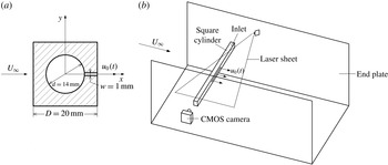
, the flow was of good quality. The experimental apparatus mainly included three parts: experimental model, synthetic jet excitation system and particle image velocimetry (PIV) system. The experimental model was a hollow square cylinder made of stainless steel with a side width
 $D=20$
mm and a span length
 $L=430$
mm. The cylindrical cavity inside was 14 mm in diameter, which was connected with the synthetic jet system. The cross-section shape at mid-span of the square cylinder is shown in figure 1(a). The origin of the coordinate system is located at the centre of the cross-section. The free stream flows towards the
 $+x$
direction. The vertical and spanwise directions are designated by
 $y$
-axis and
 $z$
-axis, respectively. A slot spanning in the range of
 $-2.5\leqslant z/D\leqslant 2.5$
with a length
 $l=100$
mm and a width
 $w=1$
mm was machined along the centreline on the rear surface of the square cylinder. Although the 3-D effects associated with the finite slot length did exist, the wake vortex-shedding modes were found to be qualitatively consistent along the span. According to previous research (Amitay & Cannelle Reference Amitay and Cannelle2006; Feng, Ma & Wang Reference Feng, Ma and Wang2014), the edge effects of the slot with the current aspect ratio were not so pronounced, especially on the flow near the mid-span regions in the near wake, where the interaction between the synthetic jet and the shear layers occurred. Our present study mainly focuses on the phenomena in these regions. End plates were used to maintain the two-dimensionality of the flow and to reduce the effects of the boundary layer developing along the channel walls on the flow field in the test section. The square cylinder was fixed on the end plates, with its axis perpendicular to the free stream and 310 mm away from the leading edge of the end plates.
(a) Schematic of the cross-section of the experimental square cylinder, (b) schematic of the experimental set-up.

The synthetic jet excitation system included computer, servo electromotor, eccentric disk, piston and so on. The servo electromotor received the sinusoidal signals exported by the computer and performed the circular motion together with the eccentric disk. The rotary motion was then transformed into the reciprocating motion of the piston via connecting rods. The outer diameter of the piston was
 $D_{p}=29$
mm. The excitation system was connected to the inlet end of the square cylinder by an ‘L’-shaped hollow cylinder. Thus the fluid inside the cylindrical cavity was injected and sucked through the slot periodically, resulting in the formation of the synthetic jet vortex pairs. The excitation frequency
 $f_{e}$
of the synthetic jet could be altered by adjusting the rotation speed of the servo electromotor.
The 2-D time-resolved PIV system was composed of computer, laser and high-speed CMOS camera. A continuous laser with output power of 5 W and wavelength of 532 nm was used to illuminate the flow field. The laser sheet perpendicular to the axis of the cylinder was fixed on the mid-span of the slot. The tracing particles were hollow glass beads with diameter
 $5{-}20~\unicode[STIX]{x03BC}\text{m}$
and density
 $1.05~\text{g}~\text{cm}^{-3}$
. A high-speed CMOS camera with a spatial resolution of 2048
 $\times$
2048 pixels was used to capture the particle images. The focal length of the lens used was 90 mm, and the corresponding field of view was in the range of
 $-2.5\leqslant x/D\leqslant 10.5$
(streamwise direction) and
 $-6.5\leqslant y/D\leqslant 6.5$
(vertical direction). Since the synthetic jet exit velocity became higher with the increase of the excitation frequency, the sampling frequency of the camera was increased gradually. The lowest sampling frequency was 100 Hz, and the highest one was 250 Hz. The exposure time was no longer than 5 ms. There were 5400 frames captured continuously at any one time and at least 10 800 snapshots were recorded for each case to enlarge the whole ensemble. The multi-pass iterative Lucas–Kanade (MILK) algorithm was applied to analyse the 8-bit particle images and to obtain the velocity vector fields (Champagnat et al.
Reference Champagnat, Plyer, Le Besnerais, Leclaire, Davoust and Le Sant2011). The size of the interrogation window was set to 32
 $\times$
32 pixels with a 75 % overlap.
The water temperature remained at
 $20\,^{\circ }\text{C}$
under the experimental conditions. The density of water at this temperature is
 $\unicode[STIX]{x1D70C}=998~\text{kg}~\text{m}^{-3}$
and the kinematic viscosity coefficient is
 $\unicode[STIX]{x1D708}=1.005\times 10^{-6}~\text{m}^{2}~\text{s}^{-1}$
. The Reynolds number based on the side length of the cylinder is
 $Re_{D}=U_{\infty }D/\unicode[STIX]{x1D708}=836$
. Considering the incompressibility of the working fluid and the acceptable 2-D characteristics of the synthetic jet, the instantaneous velocity at the synthetic jet exit can be estimated by
 $$\begin{eqnarray}\displaystyle u_{0}(t)=\frac{\unicode[STIX]{x03C0}^{2}D_{P}^{2}}{2lw}Af_{e}\sin (2\unicode[STIX]{x03C0}f_{e}t), & & \displaystyle\end{eqnarray}$$
where
 $A$
is the offset distance of the eccentric disk and
 $t$
is the excitation time. The time-averaged injection velocity during one whole cycle can be calculated by
 $$\begin{eqnarray}\displaystyle \overline{U_{0}}=\frac{1}{T}\int _{0}^{T/2}u_{0}(t)\,\text{d}t, & & \displaystyle\end{eqnarray}$$
here,
 $T=1/f_{e}$
is the cycle period. Smith & Glezer (Reference Smith and Glezer1998) proposed two primary dimensionless parameters to distinguish the synthetic jet. The first one was the dimensionless stroke length, which is the displacement of the jet moving at the exit velocity during the blowing stroke normalized by the width of the slot and is given by
 $$\begin{eqnarray}\displaystyle L_{0}/w=\frac{1}{w}\int _{0}^{T/2}u_{0}(t)\,\text{d}t=\frac{\unicode[STIX]{x03C0}AD_{p}^{2}}{2lw^{2}}, & & \displaystyle\end{eqnarray}$$
here,
 $L_{0}/w=72.6$
was obtained. The second one was the Reynolds number
 $Re_{\overline{U_{0}}}$
based on
 $\overline{U_{0}}$
, which is defined as
 $$\begin{eqnarray}\displaystyle Re_{\overline{U_{0}}}=\frac{\overline{U_{0}}w}{\unicode[STIX]{x1D708}}=\frac{\unicode[STIX]{x03C0}D_{p}^{2}Af_{e}}{2l\unicode[STIX]{x1D708}}. & & \displaystyle\end{eqnarray}$$
The definitions of the dimensionless stroke length
 $L_{0}/w$
and the Reynolds number
 $Re_{\overline{U_{0}}}$
were also adopted in previous studies (Amitay & Cannelle Reference Amitay and Cannelle2006; Feng & Wang Reference Feng and Wang2010; Feng et al.
Reference Feng, Wang and Pan2011).
In our current study, the offset distance of the eccentric disk was fixed at
 $A=5.5$
mm, thus the dimensionless stroke length
 $L_{0}/w$
was maintained as constant. The only variable parameter was the excitation frequency
 $f_{e}$
, we changed
 $f_{e}$
to alter the Reynolds number
 $Re_{\overline{U_{0}}}$
, which was proved to be associated with the vortex strength (Shuster & Smith Reference Shuster and Smith2007). Without control, the wake vortex-shedding frequency was
 $f_{0}=0.3$
Hz, the dimensionless frequencies for the control cases were selected at
 $f_{e}/f_{0}=0.5$
, 1, 2, 3, 4, 6, respectively. The corresponding Reynolds numbers were
 $Re_{\overline{U_{0}}}=11$
, 22, 43, 65, 87 and 130, respectively.
Comparable values of
 $Re_{D}$
,
 $L_{0}/w$
,
 $f_{e}/f_{0}$
and
 $Re_{\overline{U_{0}}}$
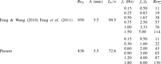
were adopted in the experiments of Feng & Wang (Reference Feng and Wang2010) and Feng et al. (Reference Feng, Wang and Pan2011). For convenience of comparison, these parameters are listed in table 1 together with those of the present study.
Experimental parameters for the control cases in the present paper and those in Feng & Wang (Reference Feng and Wang2010) and Feng et al. (Reference Feng, Wang and Pan2011).

3 Experimental results and discussion
3.1 Statistical characteristics of flow field
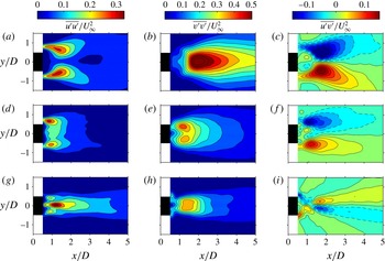
The time-averaged Reynolds stresses are displayed in figure 2. The distribution of the time-averaged streamwise Reynolds normal stress
 $\overline{u^{\prime }u^{\prime }}/U_{\infty }^{2}$
for the natural case presents a double-peak pattern with a maximum of 0.32. A similar pattern is shown for the case of
 $f_{e}/f_{0}=3$
, where the peaks are located more upstream and peak values do not change much compared with the natural case. For
 $f_{e}/f_{0}=6$
, however,
 $\overline{u^{\prime }u^{\prime }}/U_{\infty }^{2}$
exhibits a triple-peak distribution. Due to the strong blowing and suction effect of the synthetic jet, the peak on the centreline is much higher than those on both sides. The maximum of
 $\overline{u^{\prime }u^{\prime }}/U_{\infty }^{2}$
reaches 0.38, higher than the above two cases.
Time-averaged Reynolds stress distributions:
 $\overline{u^{\prime }u^{\prime }}/U_{\infty }^{2}$
,
 $\overline{v^{\prime }v^{\prime }}/U_{\infty }^{2}$
and
 $\overline{u^{\prime }v^{\prime }}/U_{\infty }^{2}$
for the natural (a–c),
 $f_{e}/f_{0}=3$
(d–f) and
 $f_{e}/f_{0}=6$
(g–i) cases. Contour intervals: (a,d,g)
 $\pm$
0.05, (b,e,h)
 $\pm$
0.05, (c,f,i)
 $\pm$
0.02.

The maxima of the time-averaged vertical Reynolds normal stress
 $\overline{v^{\prime }v^{\prime }}/U_{\infty }^{2}$
are 0.65, 0.44, 0.40 respectively for the natural case, the cases of
 $f_{e}/f_{0}=3$
and
 $f_{e}/f_{0}=6$
, decreasing as the excitation frequency increases. For the natural case, because the wake vortices from the upper and lower shear layers pass through almost the same position close to the centreline, the distribution of
 $\overline{v^{\prime }v^{\prime }}/U_{\infty }^{2}$
reveals a single-peak pattern with its peak located near
 $x/D=1.95$
. For the control case of
 $f_{e}/f_{0}=3$
, due to the interaction between the synthetic jet vortices and the shear layers, wake vortices have formed before reaching the centreline. Thus the distribution of
 $\overline{v^{\prime }v^{\prime }}/U_{\infty }^{2}$
turns out to be a double-peak pattern, and the peak is situated near
 $x/D=1.15$
, where the wake vortices detach from the shear layers (see figure 13
c). The distribution of
 $\overline{v^{\prime }v^{\prime }}/U_{\infty }^{2}$
for
 $f_{e}/f_{0}=6$
shows a plateau, which can be closely related to the behaviour of the synthetic jet vortex pair.
All the distributions of the time-averaged Reynolds shear stress
 $\overline{u^{\prime }v^{\prime }}/U_{\infty }^{2}$
are antisymmetric about the centreline. And the peak value of
 $\overline{u^{\prime }v^{\prime }}/U_{\infty }^{2}$
also decreases with the increase of the excitation frequency. For the natural case, the maximum absolute value is 0.18, located on the streamwise station of
 $x/D=1.7$
. In the region before
 $x/D=1.3$
, which is later proved in the recirculation region of the square cylinder (see figure 16
a),
 $\overline{u^{\prime }v^{\prime }}/U_{\infty }^{2}$
is positive above the centreline and negative below the centreline, while it is reverse outside of the recirculation region. This four-quadrant-type distribution induced by wake vortices was also captured in the research of flow over a circular cylinder (Balachandar, Mittal & Najjar Reference Balachandar, Mittal and Najjar1997; Kim, Yoo & Sung Reference Kim, Yoo and Sung2006). For
 $f_{e}/f_{0}=3$
, the Reynolds shear stress congregates in a smaller region. Its peaks move upstream near
 $x/D=1.1$
with the maximum absolute value reduced to 0.14. The strong synthetic jet causes a very different pattern for
 $f_{e}/f_{0}=6$
. The shear stress distributed outside of the recirculation region (shown in figure 16
b) has a negative value on the top and a positive one on the bottom before
 $x/D=1.2$
, while the distribution is opposite after
 $x/D=1.2$
. This distribution difference is caused by the synthetic jet.
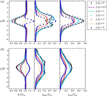
Figure 3 shows the profiles of velocity statistics measured at the streamwise stations of
 $x/D=2.5$
and
 $x/D=10$
for all the cases. For the natural case (
 $f_{e}/f_{0}=0$
), a mean streamwise velocity deficit appears in the wake due to the flow separation and the blockage effect of the cylinder. The maximum velocity deficit is smaller at
 $x/D=10$
than that at
 $x/D=2.5$
. For the control cases of
 $f_{e}/f_{0}\leqslant 3$
, the profiles of mean streamwise velocity are the wake distributions. Although the variation of velocity deficit with the excitation frequency seems irregular at
 $x/D=2.5$
, the maximum velocity deficits are all larger than that for the natural case. At
 $x/D=$
10, however, these values are all smaller under the control of the synthetic jet, and the maximum velocity deficit decreases with the increase of the excitation frequency. Thus it is manifest that the synthetic jet can accelerate the recovery of the velocity deficit. For the cases of
 $f_{e}/f_{0}=4$
, 6, more momentum is injected into the wake by the synthetic jet. Consequently, an obvious peak appears near the centreline of the mean streamwise velocity profiles at
 $x/D=2.5$
, which means that the flow tends to have a jet-like distribution. Further downstream, at
 $x/D=10$
, the peak values near the centreline decrease. The mean streamwise velocity is close to the free stream for the case of
 $f_{e}/f_{0}=4$
, but still remains with a jet-like distribution for the case of
 $f_{e}/f_{0}=6$
. Similar effects of the synthetic jet on the time-averaged streamwise velocity were obtained by Feng & Wang (Reference Feng and Wang2010) in the near wake of the circular cylinder. The velocity deficit decreases as the excitation frequency increases. The jet-like characteristic appears at
 $f_{e}/f_{0}\geqslant 2.50$
and
 $f_{e}/f_{0}=6$
for the circular cylinder and the square cylinder, respectively. It can thus be concluded that the circular cylinder wake is easier to control than the square cylinder wake.
Profiles of velocity statistics at different streamwise locations: (a)
 $x/D=2.5$
; (b)
 $x/D=10$
. Left column, mean streamwise velocity
 $U$
; middle column, root mean square of the streamwise velocity fluctuation
 $u_{rms}$
; right column, root mean square of the vertical velocity fluctuation
 $v_{rms}$
.

At
 $x/D=2.5$
, the profiles of the streamwise velocity fluctuation intensity exhibit a double peak for the cases of
 $0\leqslant f_{e}/f_{0}\leqslant 3$
, corresponding to the upper and lower separated shear layers. It is worth noticing that the streamwise turbulence intensity, as well as the peak value, is relatively small for
 $f_{e}/f_{0}=3$
, which is associated with the upstream movement of vortex shedding. The wake vortices gradually dissipate as they convect downstream, as a result, the two peaks almost disappear and the streamwise velocity fluctuation intensity decreases at
 $x/D=10$
. For the cases of
 $f_{e}/f_{0}=4,6$
, profiles of the streamwise velocity fluctuation intensity have only one peak and are symmetric about the centreline at
 $x/D=2.5$
. The streamwise turbulence intensity for
 $f_{e}/f_{0}=6$
is higher than that for
 $f_{e}/f_{0}=4$
near the centreline. Both of the streamwise fluctuations are weakened at
 $x/D=10$
due to the attenuation of the synthetic jet strength.
Only single peaks appear in the profiles of vertical velocity fluctuation intensity. It is evident that the vertical fluctuation can be reduced by means of the synthetic jet. For the cases of
 $0\leqslant f_{e}/f_{0}\leqslant 3$
, the vertical fluctuation intensity decreases monotonically with an increase of the excitation frequency. The profile with the lowest vertical fluctuation corresponds to the case of
 $f_{e}/f_{0}=4$
. The vertical fluctuation gets higher as the dimensionless excitation frequency
 $f_{e}/f_{0}$
is increased to 6, and it shows a significant decrease from
 $x/D=2.5$
to
 $x/D=10$
for all the cases.
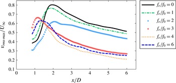
Figure 4 presents the streamwise variation of the maximum vertical velocity fluctuation
 $v_{rms\cdot max}$
. For each case, the
 $v_{rms\cdot max}$
increases first and then decreases. And the peak values of
 $v_{rms\cdot max}$
for all the control cases are reduced compared with the natural case. In addition, the peaks of the profiles for the cases of
 $f_{e}/f_{0}\geqslant 3$
are located more upstream than that for the natural case, suggesting that the wake vortices are formed much closer to the square cylinder. As the excitation frequency increases, the variation of
 $v_{rms\cdot max}$
after
 $x/D=2.1$
in figure 4 is found to be similar to that of
 $v_{rms}$
at
 $x/D=2.5$
and 10 in figure 3.
Variation of maximum vertical velocity fluctuation
 $v_{rms\cdot max}/U_{\infty }$
with streamwise locations.

The significant changes of flow structures at different excitation frequencies lead to the considerable variation in the velocity profiles, and the drag characteristics of the square cylinder are also changed. Antonia & Rajagopalan (Reference Antonia and Rajagopalan1990) used the time-averaged velocity profiles in the wake to calculate the drag coefficient
 $C_{d}$
. The formula is given by
 $$\begin{eqnarray}\displaystyle C_{d}=2\int _{-\infty }^{\infty }\frac{U}{U_{\infty }}\frac{U_{\infty }-U}{U_{\infty }}\,\text{d}\left(\frac{y}{D}\right)+2\int _{-\infty }^{\infty }\frac{\overline{v^{2}}-\overline{u^{2}}}{U_{\infty }^{2}}\,\text{d}\left(\frac{y}{D}\right), & & \displaystyle\end{eqnarray}$$
where the first item (
 $I_{1}$
) on the right-hand side is the momentum integral, and the second item (
 $I_{2}$
) represents the contribution from the Reynolds normal stresses.
 $U_{\infty }$
is the free-stream velocity.
 $U$
is the local mean velocity.
 $u$
and
 $v$
are the streamwise and vertical velocity fluctuations, respectively. Since the velocity at infinity cannot be measured in the experiment, the integral interval is chosen from
 $-6.5D$
to
 $6.5D$
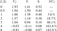
in the vertical direction where the velocity has been convergent. Drag coefficients are calculated at
 $x/D=10$
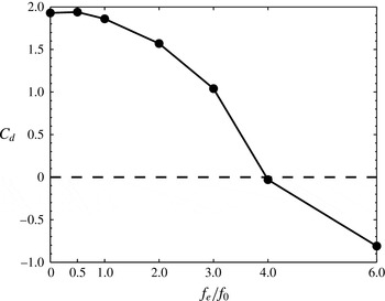
for various excitation frequencies, as shown in table 2. Figure 5 illustrates the variation of the drag coefficient
 $C_{d}$
with the dimensionless excitation frequency
 $f_{e}/f_{0}$
.
Variation of drag coefficient
 $C_{d}$
with dimensionless excitation frequency
 $f_{e}/f_{0}$
.

Drag coefficients at
 $x/D=10$
at different excitation frequencies.
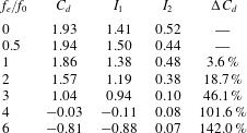
The drag coefficient
 $C_{d}$
for the natural case is 1.93, very close to the value of
 $C_{d}=1.95$
at
 $Re=1035$
in the experiment of He et al. (Reference He, Li and Wang2014). Although
 $C_{d}$
increases slightly (0.5 %) for
 $f_{e}/f_{0}=0.5$
, the drag can be considered unvaried in view of measurement uncertainty. Both
 $I_{1}$
and
 $I_{2}$
generally diminish as the excitation frequency increases, therefore, the total drag coefficient decreases and a significant drag reduction is achieved. The drag value reduces by 46.1 % for
 $f_{e}/f_{0}=3$
compared with the natural case. For the cases of
 $f_{e}/f_{0}=4$
, 6, where the wake is dominated by the synthetic jet, the drag coefficient
 $C_{d}$
is less than 0, indicating that a thrust is obtained due to the synthetic jet.
3.2 Wake vortex dynamics
3.2.1 Power spectrum analysis
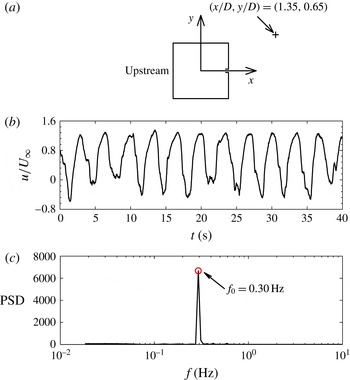
As seen in figure 6(a), a point is selected in the upper shear layer for the natural case where the root mean square of the streamwise velocity fluctuation
 $u_{rms}$
is maximal. Then the time history of the streamwise velocity at this point is extracted (figure 6
b) and a fast Fourier transformation (FFT) is used to obtain the power spectral density (PSD). The definition of the PSD function is defined with reference to Hosseini, Bourgeois & Martinuzzi (Reference Hosseini, Bourgeois and Martinuzzi2013). As shown in figure 6(c), the natural vortex-shedding frequency is
 $f_{0}=0.30$
Hz with an absolute uncertainty of
 $\pm$
0.02 Hz, corresponding to the Strouhal number
 $St=f_{0}D/U_{\infty }=0.14$
, which is consistent with the value obtained by He et al. (Reference He, Li and Wang2014).
Spectral analysis of the streamwise velocity at the point of
 $u_{rms\cdot max}$
in the upper shear layer for the natural case. (a) Location of the point
 $u_{rms\cdot max}$
, (b) time history of the streamwise velocity at
 $u_{rms\cdot max}$
, (c) power spectral density function of the streamwise velocity at
 $u_{rms\cdot max}$
.

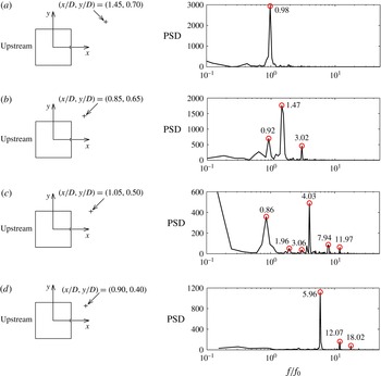
Figure 7 shows the power spectral density functions measured at the location of
 $u_{rms\cdot max}$
in the upper shear layer for several control cases, which illustrates the variation of vortex shedding frequency influenced by the synthetic jet disturbances. However, the FFT method can only represent the perturbation at one point. Ma et al. (Reference Ma, Feng, Pan, Gao and Wang2015) proposed a Fourier mode decomposition (FMD) algorithm based on the single-point discrete Fourier transformation (DFT) to give a global view of the dynamic information in a complex flow. As effective as dynamic mode decomposition (DMD), the FMD method decomposes the time-resolved data into a series of flow modes that can usually be linked to the coherent structures, according to the frequency characteristics shown on the global power spectrum which is a statistic term of the power spectrum for all the sampling points in the flow field. However, the calculation speed is accelerated for this method and it is thus more time saving. More details about the FMD algorithm can be found in the work of Ma et al. (Reference Ma, Feng, Pan, Gao and Wang2015).
Locations of the point
 $u_{rms\cdot max}$
in the upper shear layer and the corresponding power spectral density functions of the streamwise velocity at different excitation frequencies: (a)
 $f_{e}/f_{0}=2$
; (b)
 $f_{e}/f_{0}=3$
; (c)
 $f_{e}/f_{0}=4$
; (d)
 $f_{e}/f_{0}=6$
.

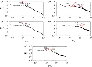
In our present study, the FMD method is applied to analyse the frequency characteristics of the global flow under the influence of the synthetic jet. For each case, the instantaneous flow fields were recorded with a high enough sampling frequency to make sure that the flow structures can be well resolved in the time dimension. Figure 8 shows the FMD spectra of the whole measured field for various excitation frequencies. With no control (figure 8
a), the spectrum shows a peak value at
 $f/f_{0}=0.98$
, illustrating that the dominant frequency is near the natural vortex-shedding frequency
 $f_{0}$
, in agreement with the FFT result. There are also small peaks near the locations of
 $2f_{0}$
and
 $3f_{0}$
. Pan, Yu & Wang (Reference Pan, Yu and Wang2011) interpreted these as high-order harmonics in their analysis of DMD, which correspond to the small-amplitude perturbations due to the sweeping and rolling effect of large-scale vortices.
FMD spectra at different excitation frequencies: (a)
 $f_{e}/f_{0}=0$
; (b)
 $f_{e}/f_{0}=2$
; (c)
 $f_{e}/f_{0}=3$
; (d)
 $f_{e}/f_{0}=4$
; (e)
 $f_{e}/f_{0}=6$
.

For
 $f_{e}/f_{0}=2$
, no apparent changes of the FFT and FMD results are observed compared to the natural case. This indicates that the control effect of the synthetic jet is weak in this case, thus the vortex-shedding frequency in figure 7(a) and the dominant frequency in figure 8(b) have not been affected and remain at approximately
 $f_{0}$
.
The vortex synchronization at half of the excitation frequency occurs for the case of
 $f_{e}/f_{0}=3$
. The vortex-shedding frequency and the dominant frequency are no longer
 $f_{0}$
, a prominent peak appears near the location of
 $1.5f_{0}$
. Besides, the spectra of FFT and FMD exhibit another noteworthy peak at
 $f/f_{0}=0.92$
, which means the perturbations induced by the natural vortex shedding still exist in the flow.
For the spectrum at the point
 $u_{rms\cdot max}$
shown in figure 7(c), the dominant frequency is approximated by the excitation frequency
 $4f_{0}$
for the case of
 $f_{e}/f_{0}=4$
. Although harmonics appear near the integral multiples of the natural vortex-shedding frequency,
 $2f_{0}$
and
 $3f_{0}$
, these peak values are smaller than those at the corresponding multiples of the excitation frequency. The high-frequency disturbances caused by the synthetic jet take over the inherent low-frequency disturbances and become the main inducement of flow instability. Moreover, the global power spectrum in figure 8(d) also has a dominant frequency of
 $4f_{0}$
and exhibits the characteristic frequencies of the power spectral density obtained by FFT, showing that the whole flow field has been governed by the synthetic jet.
The control effect of the synthetic jet for
 $f_{e}/f_{0}=6$
is more remarkable than that for
 $f_{e}/f_{0}=4$
. Both the spectrum at the single point (figure 7
d) and the FMD spectrum for the whole flow field (figure 8
e) show a dominant frequency near the excitation frequency
 $f/f_{0}=6$
. Meanwhile, its harmonics are observed and peaks below the excitation frequency disappear. In this case, the flow field is totally under the control of the synthetic jet.
The power spectral density at several points along the streamwise direction is presented in the investigation by Feng & Wang (Reference Feng and Wang2010). The natural von Kármán vortex-shedding frequency exists in the spectra for
 $f_{e}/f_{0}\leqslant 0.83$
. In our present study, however, the dominant frequency of the spectra remains the natural vortex-shedding frequency
 $f_{0}$
for
 $f_{e}/f_{0}\leqslant 2$
. This may be because the flow separation of the square cylinder, which starts from the front corners, is much stronger than that of the circular cylinder. For the square cylinder, the vortex synchronization at half of the excitation frequency occurs for
 $f_{e}/f_{0}=3$
, and the vortex shedding is locked on the excitation frequency for
 $f_{e}/f_{0}=4$
, 6. In the experiment of Feng & Wang (Reference Feng and Wang2010), the vortex synchronization at half of the excitation frequency was not observed. Vortex synchronization at the excitation frequency occurs in the range of
 $1.67\leqslant f_{e}/f_{0}\leqslant 5$
.
3.2.2 Evolution of vortex structures
Proper orthogonal decomposition (POD) is a powerful decomposition and reconstruction technique in fluid mechanics. It is frequently used to obtain the low-dimensional approximate descriptions of the high-dimensional data. The main idea of this method is to decompose the velocity signal into two independent parts: the coefficient varied with time and the POD modes orthogonal in space (Berkooz, Holmes & Lumley Reference Berkooz, Holmes and Lumley1993; Chatterjee Reference Chatterjee2000; Feng et al. Reference Feng, Wang and Pan2011). The POD modes are constructed with the eigenvectors of the velocity fluctuation autocovariance matrix and are ranked by their energy content. The large-scale coherent structures can be extracted from the flow field by the first few POD modes which carry most of the energy, at the same time, the effects of noise can be eliminated. Perrin et al. (Reference Perrin, Braza, Cid, Cazin, Moradei, Barthet, Sevrain and Hoarau2006) reported that POD is an effective approach to analyse the periodic evolution of vortices.
Strictly speaking, the wake vortex shedding behind the square cylinder is not periodic because the duration of each cycle is not the same. Therefore, when using the phase-averaging technique, the reference signal should be chosen properly in order to identify the phase of the instantaneous flow field. van Oudheusden et al. (Reference van Oudheusden, Scarano, van Hinsberg and Watt2005) proposed a phase identification method based on the first and second POD modes for quasi-periodic flow. More details can be found in the work of van Oudheusden et al. (Reference van Oudheusden, Scarano, van Hinsberg and Watt2005) and Pan, Wang & Wang (Reference Pan, Wang and Wang2013).
In the present study, the snapshot POD method (Sirovich Reference Sirovich1987; Meyer, Pedersen & Özcan Reference Meyer, Pedersen and Özcan2007) based on the streamwise and vertical velocity fluctuations is applied to analyse the evolution of vortex structures in the flow. Moreover, the time coefficients of the first two POD modes are used as the phase indicator to illustrate the periodic variation of coherent structures during the process of vortex shedding.
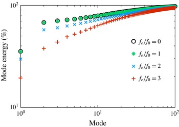
For the cases in which the drag coefficient is greater than 0, the percentage of cumulative POD mode energy to the total is shown in figure 9. It is clear that the first few modes representing the large-scale coherent structures contain most of the energy, for example, the first two modes account for nearly 70 % of the total energy for the natural case. Therefore, the shedding and convection process of wake vortices can be described by the first few modes (Dipankar, Sengupta & Talla Reference Dipankar, Sengupta and Talla2007; Feng et al.
Reference Feng, Wang and Pan2011; Baj, Bruce & Buxton Reference Baj, Bruce and Buxton2015). In our study, the spanwise vorticity is reconstructed using the first and second POD modes for the cases of
 $f_{e}/f_{0}\leqslant 3$
. For
 $f_{e}/f_{0}=1$
, the energy distribution is almost the same as that for the natural case because the synthetic jet is weak. The energy of the corresponding mode decreases as the excitation frequency increases, indicating that the control effect of the synthetic jet is enhanced and the scale of coherent structures may be reduced. Similar energy distributions were obtained by Feng et al. (Reference Feng, Wang and Pan2011) for a circular cylinder controlled by a synthetic jet.
Proportion of the accumulated POD mode energy to the total mode energy for different cases.

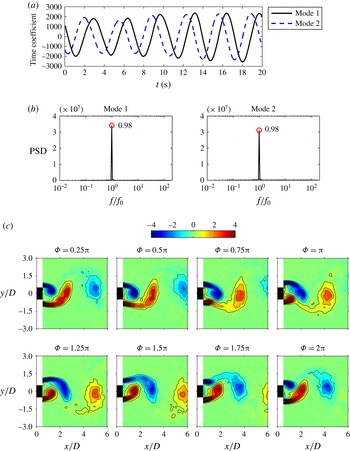
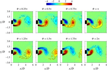
Figure 10 displays the phase-averaged results based on the first and second POD modes for the natural case. The time coefficients present similar quasi-sinusoidal variations with a phase difference (figure 10
a). The spectral analysis in figure 10(b) shows that the dominant frequency of these two sequence signals is
 $f/f_{0}=0.98$
, corresponding to the natural vortex-shedding frequency, which agrees well with the FFT and FMD results in figures 6(c) and 8(a). It can be seen from the evolution of the phase-averaged spanwise vorticity in figure 10(c) that wake vortices shed downstream antisymmetrically. During one cycle of vortex shedding, fluid is entrained into the rolling-up shear layer and grows into a vortex. The vortex develops constantly until it can draw the fluid from the other shear layer across the wake, it then detaches from the shear layer and convects downstream. A vortex with vorticity of opposite sign subsequently sheds from the shear layer on the other side after a similar process. The mechanics of the vortex formation can be found in Gerrard (Reference Gerrard1966).
Evolution of the phase-averaged spanwise vorticity
 $\unicode[STIX]{x1D714}_{z}D/U_{\infty }$
based on the first and second POD coefficients for the natural case. (a) Time histories of the first two POD coefficients, (b) power spectral density functions of the first two POD coefficients, (c) phase-averaged spanwise vorticity
 $\unicode[STIX]{x1D714}_{z}D/U_{\infty }$
at different phases in one vortex-shedding cycle. Contour intervals:
 $\pm$
0.8.

For the cases of
 $f_{e}/f_{0}=1$
and
 $f_{e}/f_{0}=2$
, the dominant frequency of the first two POD coefficients is still
 $f/f_{0}=0.98$
, near the natural vortex-shedding frequency. The evolution of the phase-averaged spanwise vorticity within one cycle for
 $f_{e}/f_{0}=1$
and
 $f_{e}/f_{0}=2$
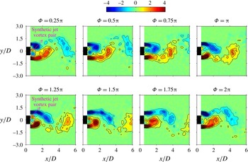
is shown in figures 11 and 12 respectively. In general, the vortex-shedding process maintains the antisymmetric mode and does not change significantly compared with the natural case. Note that for the case of
 $f_{e}/f_{0}=2$
, two excitation cycles are included in one wake vortex-shedding cycle. A synthetic jet vortex pair forms at the slot exit with a phase of
 $\unicode[STIX]{x1D6F7}=0.25\unicode[STIX]{x03C0}$
. The vorticity of the upper synthetic jet vortex is positive and the lower one is negative. Afterwards, due to the induction of the lower shear layer, the negative vorticity of the upper shear layer moves towards the centreline and merges with the negative vorticity of the synthetic jet vortex. Thus the positive vorticity of the other synthetic jet vortex is wrapped in the negative vorticity and is submerged gradually. Similarly, during the second excitation cycle, the positive vorticity of the upper synthetic jet vortex merges with that of the lower shear layer and the negative synthetic jet vortex disappears gradually. Since the synthetic jet Reynolds number
 $Re_{\overline{U_{0}}}$
is small in this case, the synthetic jet vortex pair is weak and its interaction with the shear layers is not strong enough to change the wake vortex-shedding frequency.
Evolution of the phase-averaged spanwise vorticity
 $\unicode[STIX]{x1D714}_{z}D/U_{\infty }$
based on the first and second POD coefficients for
 $f_{e}/f_{0}=1$
. Contour intervals:
 $\pm$
0.8.

Evolution of the phase-averaged spanwise vorticity
 $\unicode[STIX]{x1D714}_{z}D/U_{\infty }$
based on the first and second POD coefficients in one vortex-shedding cycle for
 $f_{e}/f_{0}=2$
. Contour intervals:
 $\pm$
0.8.

Evolution of the phase-averaged spanwise vorticity
 $\unicode[STIX]{x1D714}_{z}D/U_{\infty }$
based on the first and second POD coefficients for
 $f_{e}/f_{0}=3$
. (a) Time histories of the first two POD coefficients, (b) power spectral density functions of the first two POD coefficients, (c) phase-averaged spanwise vorticity
 $\unicode[STIX]{x1D714}_{z}D/U_{\infty }$
at different phases in one vortex-shedding cycle. Contour intervals:
 $\pm$
0.8.

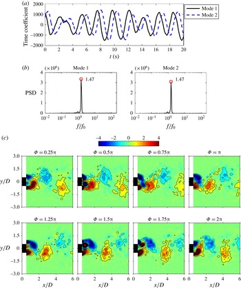
Figure 13(a,b) shows the time histories of the first two POD coefficients and their corresponding power spectral density functions for
 $f_{e}/f_{0}=3$
. The dominant frequency in figure 13(b) is
 $f/f_{0}=1.47$
, giving further evidence that synchronization at half of the excitation frequency occurs in this case. Similar to the case of
 $f_{e}/f_{0}=2$
, two excitation cycles are completed during one wake vortex-shedding cycle. The wake vortex structures present obvious changes under the influence of the synthetic jet vortices, as demonstrated in figure 13(c). At the phase of
 $\unicode[STIX]{x1D6F7}=0.25\unicode[STIX]{x03C0}$
, a counter-rotating synthetic jet vortex pair forms at the edge of the slot. But this vortex pair is not symmetric, the negative synthetic jet vortex downside is stronger than the positive one upside. Affected by the strong inducement of the positive shear layer, the negative synthetic jet vortex deflects downward and divides the lower shear layer into two parts (
 $\unicode[STIX]{x1D6F7}=0.75\unicode[STIX]{x03C0}$
). As a result, the concentrated positive vorticity detaches from the lower shear layer and rolls up into a wake vortex. At the same time, the negative vorticity of the synthetic jet vortex merges with the upper shear layer which tends to cross the centreline (
 $\unicode[STIX]{x1D6F7}=\unicode[STIX]{x03C0}$
). During the second excitation cycle, the positive synthetic jet vortex deflects upward from the centreline due to the inducement of the upper shear layer (
 $\unicode[STIX]{x1D6F7}=1.5\unicode[STIX]{x03C0}$
), hence a wake vortex with negative vorticity separates from the upper shear layer (
 $\unicode[STIX]{x1D6F7}=1.75\unicode[STIX]{x03C0}$
). Afterwards, the positive synthetic jet vortex merges with the lower shear layer (
 $\unicode[STIX]{x1D6F7}=2\unicode[STIX]{x03C0}$
). It can thus be seen that the wake vortices shed downstream with an antisymmetric mode for
 $f_{e}/f_{0}=3$
. Moreover, the process of vortex shedding is accelerated owing to the cutoff effect of the synthetic jet vortices on the shear layers. Compared with the phase-averaged spanwise vorticity for the natural case in figure 10(c), the vortex size for
 $f_{e}/f_{0}=3$
becomes much smaller, and the wake vortices are found to form closer to the square cylinder, indicating that the length of the vortex formation region is reduced by the synthetic jet.
The large-scale coherent structures are mainly concentrated in the near wake behind the square cylinder for the cases of
 $f_{e}/f_{0}=4$
and
 $f_{e}/f_{0}=6$
. The POD method is applied to decompose the velocity field in the range of
 $-0.5\leqslant x/D\leqslant 3$
,
 $-1.5\leqslant y/D\leqslant 1.5$
. Then the first six POD modes are used to reconstruct the instantaneous velocity field for these two cases, accounting for 59 % and 53 % of the total energy, respectively. Based on the reconstructed flow field, vortical structures are identified from shear layers with the
 $\unicode[STIX]{x1D706}_{ci}$
method.
 $\unicode[STIX]{x1D706}_{ci}$
is the imaginary part of the complex eigenvalue of the velocity gradient tensor (Zhou et al.
Reference Zhou, Adrian, Balachandar and Kendall1999), its rotation sense depends on the sign of the local vorticity. Figure 14 shows the instantaneous
 $\unicode[STIX]{x1D706}_{ci}$
field for
 $f_{e}/f_{0}=4$
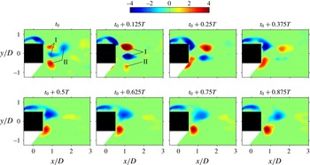
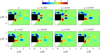
. The synthetic jet vortex pair I forms at the moment
 $t_{0}$
, then interacts with the wake vortices II which detach from the shear layers in the previous cycle, resulting in the break-up and dissipation of the wake vortices. The strength of the synthetic jet vortices is enhanced at time
 $t_{0}+0.125T$
, but attenuates gradually as they convect downstream. Induced by the synthetic jet vortex pair, vorticities accumulate near the tails of the shear layers on both sides of the square cylinder. The concentrated vorticities are found to move towards the centreline in proximity to the rear surface due to the suction of the synthetic jet. When the concentrated vorticities become large enough, they separate from the shear layers and roll up into vortex structures. Just as figure 14 shows, the flow structure in the near wake is almost symmetric but not perfectly symmetric during the evolution of the vortices.
Evolution of the instantaneous reconstructed
 $\unicode[STIX]{x1D706}_{ci}D/U_{\infty }$
field within one excitation cycle for
 $f_{e}/f_{0}=4$
.
 $T$
represents one excitation period of the synthetic jet.

As is evident from figure 15, the vortices shed symmetrically from the shear layers influenced by the symmetric perturbations of the synthetic jet for
 $f_{e}/f_{0}=6$
. Similar to the case of
 $f_{e}/f_{0}=4$
, the synthetic jet vortex pair I forms at time
 $t_{0}$
, its
 $\unicode[STIX]{x1D706}_{ci}$
value first increases and then decreases while convecting downstream. Affected by the suction stroke of the synthetic jet, the vortices II move towards the centreline in close proximity to the rear surface of the square cylinder. The vorticities III rolling up at the end of the upper and lower shear layers advect downstream gradually. At time
 $t_{0}+0.375T$
, the vortices III catch up with vortices II and they connect together. A small amount of vorticity IV drops down due to the induction of the synthetic jet vortex pair. The shear layers break off again. A new shedding vortex pair V emerges near the back corners of the square cylinder. The flow subsequently undergoes another excitation cycle. Figure 16 further displays the variation of flow structures around the square cylinder for the natural case and the case of
 $f_{e}/f_{0}=6$
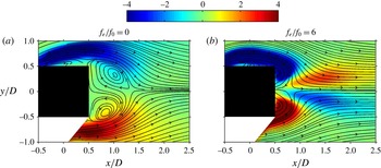
. Due to the limited spatial resolution of the PIV measurements, the flow details close to the model cannot be resolved well. Phenomena such as streamlines flowing across the square cylinder may be observed, and a similar problem was encountered in the study of van Oudheusden et al. (Reference van Oudheusden, Scarano, van Hinsberg and Watt2005). However, this does not affect our current analysis. For the natural case (figure 16
a), flow separates from the front corners, forming an obvious recirculation region behind the square cylinder. The saddle point at the end of the recirculation region is located at approximately
 $x/D=1.3$
. For
 $f_{e}/f_{0}=6$
, however, the saddle point moves upstream to the location of
 $x/D=0.8$
. The mean recirculation region thus becomes shorter in length than that for the natural case. In this case, the streamlines in the shear layer are much closer to the side surface and almost reattach to the rear surface of the square cylinder. The separation is suppressed effectively.
Evolution of the instantaneous reconstructed
 $\unicode[STIX]{x1D706}_{ci}D/U_{\infty }$
field within one excitation cycle for
 $f_{e}/f_{0}=6$
.
 $T$
represents one excitation period of the synthetic jet.

Time-averaged streamlines superimposed on time-averaged spanwise vorticity
 $\unicode[STIX]{x1D714}_{z}D/U_{\infty }$
around the square cylinder. (a) Natural, (b)
 $f_{e}/f_{0}=6$
.

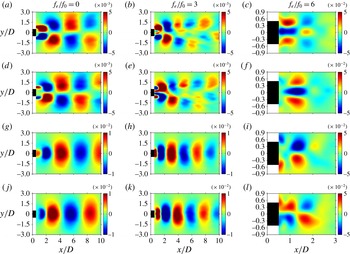
To assist the interpretation of the variation in flow structures under the synthetic jet actuation, figure 17 presents the spatial distributions of the first two POD modes which can be directly linked to the wake vortices. For the POD modes based on the streamwise velocity, usually, the antisymmetric distributions represent the antisymmetric vortex-shedding modes, while the symmetric distributions correspond to the symmetric shedding process. However, the relation between the POD modes based on the vertical velocity and the vortex-shedding modes is just the opposite (Feng et al.
Reference Feng, Wang and Pan2011). For the natural case, the signs of structures shown in figure 17 vary alternately. The POD modes based on the streamwise velocity and the vertical velocity are antisymmetric and symmetric about the centreline respectively, representing the antisymmetric vortex-shedding mode. The flow patterns presented by the first and second POD modes are in good agreement with those obtained by He et al. (Reference He, Li and Wang2014). Since the distributions of the first two POD modes do not change for
 $f_{e}/f_{0}=3$
, the wake vortices still shed downstream antisymmetrically. However, the scales of the coherent structures are smaller than those for the natural case, which can also be validated by the phase-averaged spanwise vorticity in figure 13(c). When the excitation frequency is increased to
 $f_{e}/f_{0}=6$
, the first and second POD modes based on the streamwise velocity are symmetric about the centreline while the modes based on the vertical velocity are antisymmetric. The size of the coherent structures becomes much smaller. It is reasonable to infer that the synthetic jet plays a dominant role in the wake for
 $f_{e}/f_{0}=6$
, and the wake flow becomes symmetric as a result of the strong symmetric perturbations introduced by the synthetic jet.
The first and second modes of the proper orthogonal decomposition. (a–c) The first mode of streamwise component, (d–f) the second mode of streamwise component, (g–i) the first mode of vertical component, (j–l) the second mode of vertical component.

In general, the states of wake vortex shedding change from the antisymmetric mode to the symmetric mode as the excitation frequency increases in the present study for a square cylinder. Feng et al. (Reference Feng, Wang and Pan2011) obtained a similar result in their investigation of a circular cylinder. However, the ranges of dimensionless excitation frequency corresponding to the symmetric modes are different for each bluff body. Another difference is reflected in the transition state of vortex shedding. For the square cylinder, the transition state happens when
 $f_{e}/f_{0}=3$
, the power spectra of the first two POD modes show a peak value of half of the excitation frequency and wake vortices shed downstream antisymmetrically. While the transition state for the circular cylinder occurs when
 $f_{e}/f_{0}=1.67$
, the dominant frequency of the first two POD modes is near the natural shedding frequency, both the antisymmetric shedding mode and the symmetric one were observed in this case.
4 Conclusions
The wake vortex evolution of a square cylinder controlled by a slot synthetic jet positioned at the rear surface has been investigated experimentally with the particle image velocimetry technique. The time-averaged Reynolds stress distributions, the velocity statistics in the wake and the drag reduction are compared at different excitation frequencies of the synthetic jet. The FFT and FMD methods are applied to analyse the frequency characteristics of the flow field, while the POD analysis is adopted to extract the large-scale coherent structures. Phase averaging based on the first and second POD modes and the POD reconstruction technique provide efficient tools for understanding the evolution of spanwise vortices. The following conclusions have been drawn.
The peaks of the time-averaged Reynolds stresses for
 $f_{e}/f_{0}=3$
appear more upstream than those for the natural case, illustrating that the interaction between the synthetic jet and the shear layers shortens the wake vortex formation length. When the excitation frequency is increased to
 $f_{e}/f_{0}=6$
, the distributions of the Reynolds stresses present significant changes due to the strength enhancement of the synthetic jet. The slot synthetic jet issuing from the rear surface of the square cylinder can accelerate the recovery of the mean streamwise velocity deficit and reduce the vertical velocity fluctuation intensity. For the control cases of
 $0\leqslant f_{e}/f_{0}\leqslant 3$
, the profiles of the mean streamwise velocity are the wake distributions, and the profiles of the streamwise velocity fluctuation intensity exhibit a double peak in the near wake. While for the cases of
 $f_{e}/f_{0}=4$
and
 $f_{e}/f_{0}=6$
, profiles of the mean streamwise velocity tend to have jet-like distributions and only one peak exists on the profiles of the streamwise velocity fluctuation intensity at
 $x/D=2.5$
. It is found that the synthetic jet has a remarkable effect on drag reduction. In general, the drag coefficient decreases with an increase in the excitation frequency. A drag reduction of 46.1 % is achieved for
 $f_{e}/f_{0}=3$
compared with the natural case. A thrust instead of drag reduction is obtained for
 $f_{e}/f_{0}=4$
and
 $f_{e}/f_{0}=6$
.
On the aspect of frequency characteristics, the peak frequency based on the spectral analysis at one point is consistent with the dominant frequency resolved by the FMD algorithm for the global flow. The wake vortex-shedding frequency for
 $f_{e}/f_{0}=0.5$
, 1, 2 is the same as that for the natural case. The vortex shedding is locked on half of the excitation frequency for
 $f_{e}/f_{0}=3$
. While the wake vortex shedding is synchronized with the synthetic jet excitation for
 $f_{e}/f_{0}=4$
and
 $f_{e}/f_{0}=6$
.
As for the evolution of vortex structures, for the control cases of
 $f_{e}/f_{0}\leqslant 2$
, because the synthetic jet is weak, the wake vortex structures do not change significantly. For
 $f_{e}/f_{0}=3$
, the wake vortices still shed downstream with an antisymmetric mode. The synthetic jet vortex deflects to one side due to the inducement of the shear layer. The interaction between the synthetic jet vortices and the shear layers accelerates the vortex-shedding process. Also, the wake vortices are found to form much closer to the square cylinder and their scales are significantly reduced. For
 $f_{e}/f_{0}=6$
, after rolling up from the upper and lower shear layers, the wake vortices move towards the centreline in close proximity to the rear surface of the square cylinder. The concentrated spanwise vorticities at the end of the shear layers shed symmetrically influenced by the symmetric perturbations of the synthetic jet. The mean recirculation region is shorter in length compared with that for the natural case and the flow separation is suppressed effectively.
Similarities and differences are compared between the control effect of synthetic jet on a square cylinder and a circular cylinder. For each bluff body, the synthetic jet gradually changes the wake vortex characteristics as the excitation frequency increases and finally dominates the global flow field. The wake vortex shedding is eventually locked on the excitation frequency and is converted from the original antisymmetric mode to the symmetric one. However, due to the different characteristics of flow separation, some flow details, such as the transition state of wake vortex shedding and the excitation frequency corresponding to the symmetric vortex-shedding mode, can be different. The square cylinder wake is more difficult to control than the circular cylinder wake.
Acknowledgements
This work was supported by the National Natural Science Foundation of China (no. 11202015) and the Fundamental Research Funds for the Central Universities (nos YWF-16-BJ-Y-06 and YWF-16-JCTD-A-05).