1 Introduction
Wall-bounded turbulent flow over rough walls occur in a wide range of engineering surfaces. In most engineering systems, roughness increases the skin-friction coefficient
 $C_{f}$
(which is the ratio between the wall shear stress
 $\unicode[STIX]{x1D70F}_{w}$
and the dynamic pressure
 $\unicode[STIX]{x1D70C}U_{b}^{2}/2$
, where
 $U_{b}$
is the bulk velocity and
 $\unicode[STIX]{x1D70C}$
the density of the fluid), which consequently decreases the efficiency of the system as additional energy is expended to overcome drag. While the effect of roughness on drag is fairly well understood, there is less understanding in terms of how surface roughness modifies turbulent flow structures, particularly in the near-wall region, and within the roughness canopy, which remain inaccessible to the majority of laboratory experiments.
1.1 Near-wall structures
The near-wall structures of a rough-wall flow depend greatly on the topological features of the surface. The differences in the flow due to two-dimensional and three-dimensional roughness have been substantially investigated (e.g. Antonia & Krogstad Reference Antonia and Krogstad2001; Orlandi & Leonardi Reference Orlandi and Leonardi2006; Volino, Schultz & Flack Reference Volino, Schultz and Flack2011). Krogstad & Antonia (Reference Krogstad and Antonia1999) conducted rough-wall experiments on a turbulent boundary layer flow over woven stainless steel mesh (three-dimensional roughness) and spanwise circular rods (two-dimensional roughness). Both of these roughnesses had a similar Hama roughness function
 $\unicode[STIX]{x0394}U^{+}$
, which is the measure of the downward shift in the scaled mean velocity profile of the rough case compared to the smooth-wall case at the equivalent Reynolds number. Despite both surfaces having similar measurements of drag, it was found that the two-dimensional circular rods had a larger effect on the outer region of the flow as there was a lack of collapse in both the wall-normal turbulence intensity and Reynolds shear stress profiles between the smooth and rough cases. De Marchis, Milici & Napoli (Reference De Marchis, Milici and Napoli2015) simulated two- and three-dimensional roughness by superposition of sinusoidal surfaces of varying roughness height and wavelength. From their simulations, they found that the streaky structures still persist near the wall but are selectively modified by the roughness. While these structures are able to meander around the three-dimensional roughness, the streamwise streaks are abruptly broken by the two-dimensional roughness elements as the infinite spanwise length of the roughness elements only allows for the fluid to flow over and not around the roughness elements.
It has also been found that the arrangements of the roughness elements can substantially change the turbulent near-wall flow. Orlandi & Leonardi (Reference Orlandi and Leonardi2006) found that when cube array roughness is ordered in a staggered arrangement, the
 $\unicode[STIX]{x0394}U^{+}$
for the rough surface is higher than the streamwise aligned cubes despite both having the same planar density.
 $\unicode[STIX]{x0394}U^{+}$
is lower for the aligned roughness due to the sheltering effect of the roughness elements where the cube element lies within the wake of the upstream cube. In addition, the alignment of the roughness creates a path of low resistance so that the flow is channelled between axial rows of cubes. When considering the streamwise vorticity, it is found that these structures exist predominantly above the crest of the cube roughness for the aligned case, whereas these structures reside deeper within the roughness canopy in the staggered case. This consequently causes an increase in the wall-normal fluctuations at the crest of the cubes for the staggered case, due to higher turbulent mixing. The work of Sadique et al. (Reference Sadique, Yang, Meneveau and Mittal2016) and Yang et al. (Reference Yang, Sadique, Mittal and Meneveau2016) explored the possibility of quantifying the effects of sheltering by developing a volumetric sheltering model for a flow over rectangular-prism-shaped roughness elements.
In recent years, large-scale spanwise heterogeneity in the roughness has been identified as causing large secondary flows which disrupt the near-wall cycle of the boundary layer. Mejia-Alvarez & Christensen (Reference Mejia-Alvarez and Christensen2013) and Barros & Christensen (Reference Barros and Christensen2014) found that the spanwise variations in the roughness height of their test surface (a damaged turbine blade due to the deposition of foreign material), which resulted in alternating regions of low and high momentum (known as high-momentum paths (HMPs) and low-momentum paths (LMPs)), caused the occurrence of secondary flows. These secondary flows are found to be ‘stress-induced’ due to the spatial gradients of the Reynolds stress components and are categorised as Prandtl’s secondary flow of the second kind (Willingham et al.
Reference Willingham, Anderson, Christensen and Barros2014; Anderson et al.
Reference Anderson, Barros, Christensen and Awasthi2015). It is generally agreed that the spanwise variation of the skin-friction velocity
 $U_{\unicode[STIX]{x1D70F}}$
(
 $\equiv \sqrt{\unicode[STIX]{x1D70F}_{w}/\unicode[STIX]{x1D70C}}$
), whether due to physical roughness or modelled in numerical simulations, induces secondary flows (Willingham et al.
Reference Willingham, Anderson, Christensen and Barros2014; Anderson et al.
Reference Anderson, Barros, Christensen and Awasthi2015; Medjnoun, Vanderwel & Ganapathisubramani Reference Medjnoun, Vanderwel and Ganapathisubramani2018). To investigate this interesting phenomenon, Vanderwel & Ganapathisubramani (Reference Vanderwel and Ganapathisubramani2015) conducted a systematic laboratory experiment to determine how and when large-scale secondary flows occur in a rough-wall turbulent boundary layer. In that study, the spanwise spacing of the roughness elements
 $l_{s}$
(streamwise aligned Lego® bricks) was varied from
 $0.3\unicode[STIX]{x1D6FF}$
to
 $1.76\unicode[STIX]{x1D6FF}$
. They found that the intensity of the secondary flows is amplified when the spanwise spacings of the roughness elements are approximately equal to
 $\unicode[STIX]{x1D6FF}$
. The roughness elements push the flow upwards and create a pair of counter-rotating streamwise vortices which affect the flow all the way to the edge of the boundary layer. Large-eddy simulations conducted by Anderson et al. (Reference Anderson, Barros, Christensen and Awasthi2015) over heterogeneous roughness also observed these large secondary flows when the spanwise spacing of the roughness is larger than
 $\unicode[STIX]{x1D6FF}$
(albeit in the opposite orientation to those of Vanderwel & Ganapathisubramani (Reference Vanderwel and Ganapathisubramani2015)). Recent work by Yang & Anderson (Reference Yang and Anderson2018) defined three regimes based on the spanwise spacing of the roughness. The surface is considered a topography when
 $l_{s}/\unicode[STIX]{x1D6FF}\gtrsim 2$
and the surface behaves as a homogeneous roughness when
 $l_{s}/\unicode[STIX]{x1D6FF}\lesssim 0.2$
. For
 $0.2\lesssim l_{s}/\unicode[STIX]{x1D6FF}\lesssim 2$
, the surface is in the intermediate regime where secondary flows exist. These studies have shown that the ratio of the spanwise length scale of the roughness heterogeneity to the boundary layer thickness is a critical parameter in determining the occurrence of secondary flows.
When investigating the turbulent flow over converging–diverging riblets, Nugroho, Hutchins & Monty (Reference Nugroho, Hutchins and Monty2013) found that these aligned surfaces completely modulate the entire boundary layer despite having a relatively small roughness height (
 $k/\unicode[STIX]{x1D6FF}\approx 0.01$
with
 $k^{+}\approx 20$
), due to the occurrence of very large and intense secondary flows. A recent study by Kevin et al. (Reference Monty, Bai, Pathikonda, Nugroho, Barros, Christensen and Hutchins2017) suggests that these converging–diverging riblet surfaces are different to the previously mentioned heterogeneous roughness, since they represent a directional heterogeneity. They postulated that there might be a different driving mechanism other than the spanwise variation in wall drag which is commonly assumed to drive the secondary flows for spanwise heterogeneous roughness.
The topographical features of a rough surface are indeed important in determining the near-wall flow structures. When conducting direct numerical simulations (DNS) or scaled laboratory experiments of a replicated roughness, the raw surface typically has to be filtered to remove any measurement noise that is likely to exist from the surface scanning process and to remove features smaller than the computational mesh. To accurately capture the behaviour of the near-wall flow, Mejia-Alvarez & Christensen (Reference Mejia-Alvarez and Christensen2010) found in their experiments that the filtered rough surface must contain the dominant 95 % of the full set of basis functions of the raw surface. Over-filtering these rough surfaces would lead to an overprediction of the mean velocity profile (Busse, Lützner & Sandham Reference Busse, Lützner and Sandham2015). This clearly indicates that the turbulent flow is sensitive to small-scale changes in the roughness topography and that any manipulation of the raw surface data has to be minimal and justified. This often makes simulating turbulent flow over rough walls at high Reynolds number computationally prohibitive. One attempt to overcome this problem is to conduct DNS in a minimal-span channel which uses a much smaller computation domain than a full-span channel (Chung et al. Reference Chung, Chan, MacDonald, Hutchins and Ooi2015; MacDonald et al. Reference MacDonald, Chung, Hutchins, Chan, Ooi and Garca-Mayoral2017). In summary, it is undeniable that the near-wall structures for turbulent flow over rough walls are very specific to the characteristic features of the surface.
1.2 Outer-layer similarity
In the outer region of the flow, Townsend (Reference Townsend1976) hypothesised that the turbulent flow is not influenced by viscosity except through the wall shear stress. An extension of Townsend’s outer-layer similarity hypothesis (in relation to rough-wall-bounded flow) proposed by Raupach, Antonia & Rajagopalan (Reference Raupach, Antonia and Rajagopalan1991) states that the outer region turbulent flow is not affected by the viscosity and the wall roughness whose only effect is to set the friction velocity of the wall, the virtual origin offset
 $\unicode[STIX]{x1D716}$
and the boundary layer thickness
 $\unicode[STIX]{x1D6FF}$
.
Throughout the years, there have been conflicting opinions on outer-layer similarity in the literature for turbulent flow over rough walls. Depending on the statistics that are being considered, there has been work on turbulent flow over rough walls where outer-layer similarity is not observed (Krogstad, Antonia & Browne Reference Krogstad, Antonia and Browne1992; Krogstad & Antonia Reference Krogstad and Antonia1994, Reference Krogstad and Antonia1999; Tachie, Bergstrom & Balachandar Reference Tachie, Bergstrom and Balachandar2000; Bhaganagar, Kim & Coleman Reference Bhaganagar, Kim and Coleman2004). On the contrary, there has also been a variety of literature which supports outer-layer similarity (Andreopoulos & Bradshaw Reference Andreopoulos and Bradshaw1981; Raupach & Shaw Reference Raupach and Shaw1982; Schultz & Flack Reference Schultz and Flack2005; Flack & Schultz Reference Flack and Schultz2014; Squire et al.
Reference Squire, Morrill-Winter, Hutchins, Schultz, Klewicki and Marusic2016). There are multiple reasons why there have been such polarising views on this matter. One of the reasons is because outer-layer similarity depends on (i) the topology of the roughness (e.g. two-dimensional versus three-dimensional roughness, roughness spanwise heterogeneity) as highlighted in § 1.1. In addition, to satisfy the requirement for outer-layer similarity, (ii) the boundary layer thickness
 $\unicode[STIX]{x1D6FF}$
has to be much larger than the roughness elements. Jiménez (Reference Jiménez2004) in his review paper suggested that the ratio of the boundary layer thickness to the roughness height
 $\unicode[STIX]{x1D6FF}/k$
has to be at least 40 for outer-layer similarity to be observed. Flack, Schultz & Shapiro (Reference Flack, Schultz and Shapiro2005) used data in the open literature and found that a good collapse in the outer region of the flow is obtained when the height of the boundary layer thickness is normalised by the uniform sandgrain roughness height
 $k_{s}$
instead of
 $k$
for values of
 $\unicode[STIX]{x1D6FF}/k_{s}\geqslant 40$
. Turbulent flows which do not meet these requirements are treated as flow over obstacles rather than a roughness. The concern with data from numerical simulations is that all currently available literature on rough-wall DNS fail to meet this requirement. Most numerical simulations of rough walls have single digit values of
 $\unicode[STIX]{x1D6FF}/k$
(Coceal et al. (Reference Coceal, Thomas, Castro and Belcher2006):
 $\unicode[STIX]{x1D6FF}/k=4$
, Chan et al. (Reference Chan, MacDonald, Chung, Hutchins and Ooi2015):
 $\unicode[STIX]{x1D6FF}/k=6.75$
, Yuan & Piomelli (Reference Yuan and Piomelli2014):
 $\unicode[STIX]{x1D6FF}/k=7.1$
, Leonardi & Castro (Reference Leonardi and Castro2010):
 $\unicode[STIX]{x1D6FF}/k=8$
, Busse et al. (Reference Busse, Lützner and Sandham2015):
 $\unicode[STIX]{x1D6FF}/k=9$
) and even the largest value of
 $\unicode[STIX]{x1D6FF}/k=25$
in work conducted by Scotti (Reference Scotti2006) is still approximately half of what is required. Despite the low
 $\unicode[STIX]{x1D6FF}/k$
of these surfaces, Townsend’s outer-layer hypothesis appears to be satisfied at least when considering the mean statistics. This is because most rough-wall numerical studies have simulated an internal flow (channels and pipes) where
 $\unicode[STIX]{x1D6FF}$
is fixed and the stress at the centre of the domain is zero. This is not the case for external flows where the boundary layers are unbounded and more sensitive to the
 $\unicode[STIX]{x1D6FF}/k$
ratio. Therefore we arrive at a third possible explanation for the apparent disparity reported for outer-layer similarity, (iii) the type of flow also seems to play a role in determining outer-layer similarity. (iv) The streamwise spacing of the roughness to boundary layer thickness,
 $l_{x}/\unicode[STIX]{x1D6FF}$
ratio is also important as large streamwise spacings can cause the development of an internal boundary layer due to the sudden change in wall shear stress (Antonia & Luxton Reference Antonia and Luxton1971). In this paper, we present some evidence which shows that outer-layer similarity also depends on the (v) roughness spanwise spacing to boundary layer thickness,
 $l_{s}/\unicode[STIX]{x1D6FF}$
ratio. This is expected as dimensional analysis requires the roughness characteristic length (roughness height and wavelengths) to be small compared to the boundary layer thickness for outer-layer similarity to be observed.
This paper is a continuation of the previous work of Chan et al. (Reference Chan, MacDonald, Chung, Hutchins and Ooi2015) who focused on the mean statistics and the influence of the wavelength and height of the roughness elements on the drag penalty of a rough surface in a turbulent pipe flow. In this paper, we investigate the effects of roughness on the turbulent flow structures when the height and wavelength of the roughness elements are systematically varied. The use of DNS, which contains both the spatial and time information of the flow in all three velocity components, allows for quantitative analysis and qualitative observations to be carried out. Throughout this manuscript, the ‘
 $+$
’ superscript indicates the viscous-scaled quantities (e.g.
 $r^{+}=rU_{\unicode[STIX]{x1D70F}}/\unicode[STIX]{x1D708}$
for length,
 $u^{+}=u/U_{\unicode[STIX]{x1D70F}}$
for velocity and
 $t^{+}=tU_{\unicode[STIX]{x1D70F}}^{2}/\unicode[STIX]{x1D708}$
for time, where
 $\unicode[STIX]{x1D708}$
is the kinematic viscosity). The cylindrical coordinate system is used where
 $x$
,
 $\unicode[STIX]{x1D703}$
and
 $r$
denote the streamwise, azimuthal and radial directions, respectively. The ‘spanwise’ (azimuthal) length in the pipe is measured along the arclength
 $s=r\unicode[STIX]{x1D703}$
.
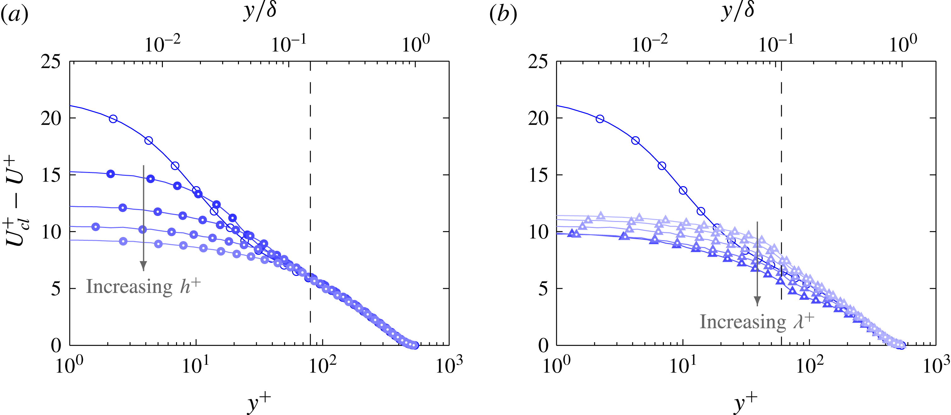
Computational details for the roughness cases.
 $N_{r,\unicode[STIX]{x1D703}}$
is the number of elements in an
 $(r,\unicode[STIX]{x1D703})$
plane,
 $N_{x}$
is the number of elements in the streamwise direction and
 $N_{\unicode[STIX]{x1D706}_{x}}$
is the number of elements per roughness wavelength.
 $\unicode[STIX]{x0394}r_{w}^{+}$
,
 $\unicode[STIX]{x0394}r\unicode[STIX]{x1D703}_{w}^{+}$
and
 $\unicode[STIX]{x0394}x_{w}^{+}$
are the mean grid spacings in wall units at the wall calculated using (the local, time averaged)
 $\overline{u}_{\unicode[STIX]{x1D70F}}$
and
 $\unicode[STIX]{x0394}t^{+}$
is the time step. The largest cells are located at the centre of the pipe where
 $\unicode[STIX]{x0394}r^{+}\approx \unicode[STIX]{x0394}r\unicode[STIX]{x1D703}^{+}\approx \unicode[STIX]{x0394}x^{+}$
. Nominal friction Reynolds number
 $Re_{\unicode[STIX]{x1D70F}}$
is shown.

2 Numerical procedure
The turbulent flows in rough-wall pipes are simulated using CDP which is a second-order, finite volume, energy conserving code (Ham & Iaccarino Reference Ham and Iaccarino2004; Mahesh, Constantinescu & Moin Reference Mahesh, Constantinescu and Moin2004). A conforming grid is used to explicitly mesh the roughness elements where the no-slip condition is applied. The inlet and outlet of the pipe are set to be periodic and the pipe has a length of
 $L_{x}=4\unicode[STIX]{x03C0}R_{0}$
, where
 $R_{0}$
is the reference radius of the pipe (which is equal to the mean radius of the pipe). The length of this domain is sufficiently long to obtain accurate mean and second-order statistics but is unable to capture the largest streamwise structures in the flow (Chin et al.
Reference Chin, Ooi, Marusic and Blackburn2010). However, as the length of the domain remains constant for all of the cases simulated, any changes to the large-scale structures are due to the influence of the roughness elements. A summary of the mesh parameters for all of the cases simulated is tabulated in table 1. The turbulent flow is simulated at a nominal friction Reynolds number of
 $Re_{\unicode[STIX]{x1D70F}}=540$
using a sufficiently fine mesh (
 ${\approx}120$
million cells per roughness case) and small time step (Courant number
 ${\leqslant}1$
) to ensure all physical and temporal length scales are fully resolved. For a turbulent flow over rough walls, the mesh not only has to resolve the wall unit,
 $\unicode[STIX]{x1D708}/u_{\unicode[STIX]{x1D70F}}$
, and the Kolmogorov length scale,
 $\unicode[STIX]{x1D702}$
, but also the topological features of the roughness (at least 24 elements per roughness wavelength,
 $N_{\unicode[STIX]{x1D706}_{x}}\geqslant 24$
). Due to the stringent computational requirements, the Reynolds number of the flow is limited so that a range of cases could be simulated. Statistics are gathered for at least 5 flow-through times
 $T=L_{x}/U_{b}$
, where
 $U_{b}$
is the bulk velocity, to ensure a sufficiently converged result. Further details of the computational domain and numerical setup can be found in Chan et al. (Reference Chan, MacDonald, Chung, Hutchins and Ooi2015).
3 Surface roughness parameters
The rough surface consists of three-dimensional sinusoidal roughness elements governed by the following equation
 $$\begin{eqnarray}R(x,\unicode[STIX]{x1D703})=R_{0}+h\cos \left(\frac{2\unicode[STIX]{x03C0}x}{\unicode[STIX]{x1D706}_{x}}\right)\cos \left(\frac{2\unicode[STIX]{x03C0}R_{0}\unicode[STIX]{x1D703}}{\unicode[STIX]{x1D706}_{s}}\right).\end{eqnarray}$$
 $h$
is the roughness semi-amplitude (half of the peak-to-trough height
 $k_{t}=2h$
) and
 $\unicode[STIX]{x1D706}_{x}$
and
 $\unicode[STIX]{x1D706}_{s}$
are the wavelengths of the roughness elements in the streamwise and azimuthal directions. For all of the rough cases simulated,
 $\unicode[STIX]{x1D706}_{x}=\unicode[STIX]{x1D706}_{s}=\unicode[STIX]{x1D706}$
. The rough cases are identified by the following identifying code

where the first two digits represent the viscous roughness height and the last three digits represent the viscous wavelength of the roughness elements. A sketch of the sinusoidal roughness for case 60_424 is presented in figure 1.
Sketch of the roughness case 60_424. The
 $x$
-axis is in the streamwise direction and the radial distance
 $r$
is measured from the centre of the pipe.
 $L_{x}$
is the length of the pipe and
 $y$
is the wall-normal direction measured from
 $R_{0}$
. Close-up sketch in (a) illustrates the streamwise and spanwise roughness wavelengths (
 $\unicode[STIX]{x1D706}_{x}$
and
 $\unicode[STIX]{x1D706}_{s}$
). Cross-sectional plane I and streamwise plane
 $A$
are the planes which are locally rough and cross-sectional plane II and streamwise plane
 $B$
are the planes which are locally smooth.
 $l_{s}$
is the spanwise roughness spacing corresponding to half the wavelength
 $\unicode[STIX]{x1D706}_{s}$
.
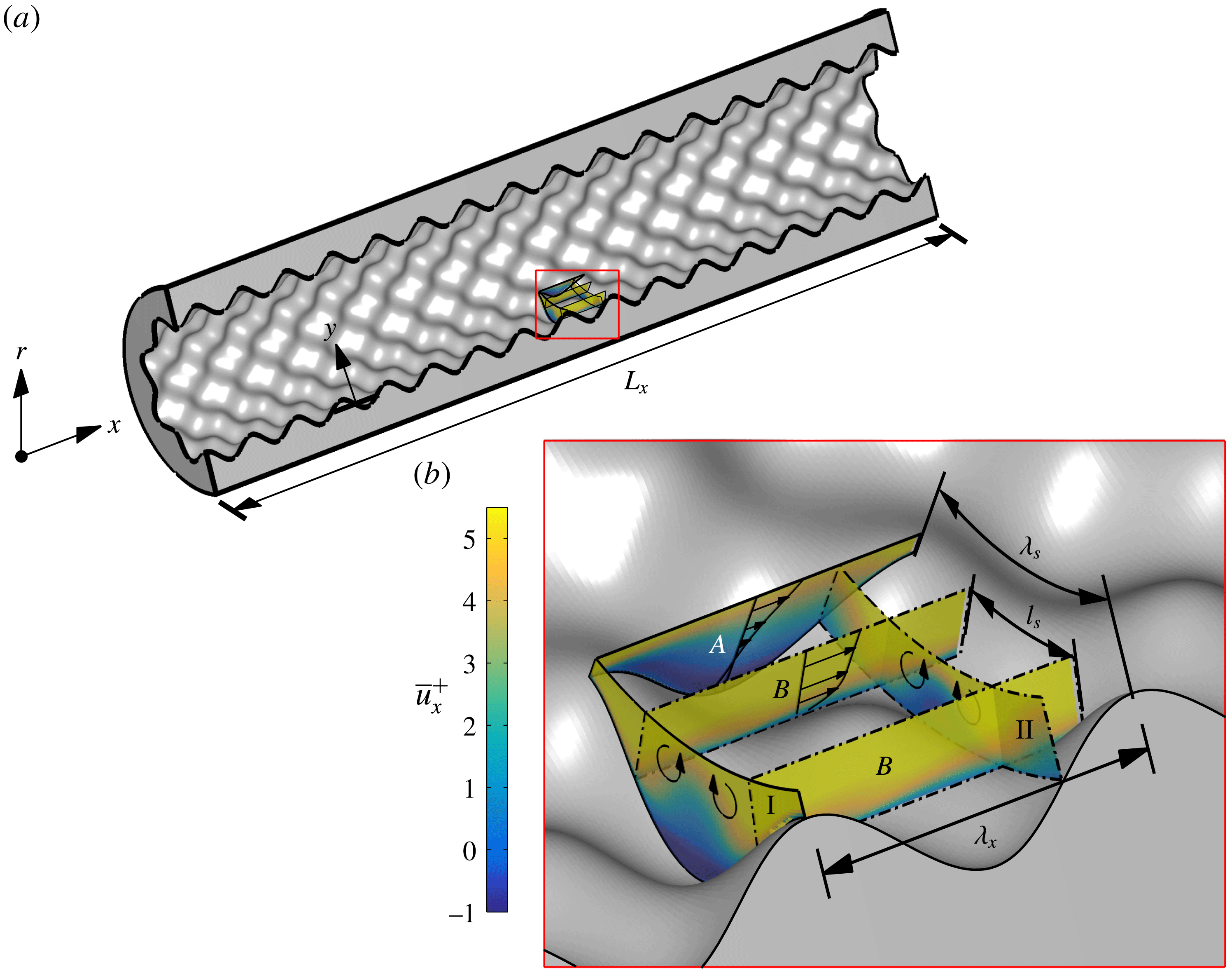
This sinusoidal roughness contains streamwise planes which are locally rough (plane
 $A$
) and locally smooth (plane
 $B$
) and cross-sectional planes which are locally rough (plane I) and locally smooth (plane II). Due to the staggered arrangement of the sinusoidal roughness elements, the spanwise spacing of the roughness is half of the roughness wavelength (
 $l_{s}=\unicode[STIX]{x1D706}_{s}/2$
) as there are two locally smooth pathways per spanwise wavelength. The sketch in figure 1(a) also shows the direction of secondary flows due to the spanwise variation of the mean streamwise velocity within the roughness canopy. As was discussed by Chan et al. (Reference Chan, MacDonald, Chung, Hutchins and Ooi2015), the virtual origin of the wall (
 $y=0$
) is set to be
 $R_{0}$
which is essentially the hydraulic radius of the pipe for the range of roughness simulated. The roughness parameters for the cases simulated are given in table 2.
 $k_{a}^{+}$
is the average roughness height which is the mean of the absolute roughness fluctuation from the mean roughness height
 $$\begin{eqnarray}k_{a}=\frac{1}{2\unicode[STIX]{x03C0}L_{x}}\int _{0}^{2\unicode[STIX]{x03C0}}\int _{0}^{L_{x}}|R(x,\unicode[STIX]{x1D703})-\overline{R}|\,\text{d}x\,\text{d}\unicode[STIX]{x1D703}\end{eqnarray}$$
and
 $k_{rms}^{+}$
is the root-mean-squared roughness height. Skewness of the roughness height
 $k_{skew}^{+}$
is zero for all of the cases simulated. The effective slope
 $ES$
, is defined as the mean of the absolute streamwise gradient and is related to solidity
 $\unicode[STIX]{x1D6EC}$
by
 $ES=2\unicode[STIX]{x1D6EC}$
(Napoli, Armenio & De Marchis Reference Napoli, Armenio and De Marchis2008). These roughness parameters are dominant factors contributing to drag and various roughness function models have been developed based on them (Flack & Schultz Reference Flack and Schultz2010; Chan et al.
Reference Chan, MacDonald, Chung, Hutchins and Ooi2015). Two groups of cases have been simulated where the roughness wavelength and height are systematically varied. The first group
 $C1$
consist of cases where the roughness elements are geometrically scaled from the transitionally rough to the fully rough regime. Typically, in laboratory experiments, turbulent flow in rough-wall pipes span from the transitionally rough regime to the fully rough regime by increasing the Reynolds number of the flow while maintaining a constant
 $\unicode[STIX]{x1D6FF}/k$
ratio. Simulating a turbulent flow at high Reynolds numbers is computationally prohibitive and therefore we have geometrically scaled our roughness elements while maintaining a constant
 $Re_{\unicode[STIX]{x1D70F}}$
. The second group
 $C2$
is where we alter the wavelength of the roughness elements while maintaining a constant roughness semi-amplitude
 $h^{+}$
. Figure 2 shows the cross-sectional sketch of the rough pipe for a range of roughness heights and wavelengths. The grey filled sketches are the cases which have been simulated in this study at
 $Re_{\unicode[STIX]{x1D70F}}=540$
. Cases 40_283 and 60_283 both have the same roughness wavelength but different roughness height and therefore different
 $ES$
.
Description of the roughness elements.
 $Re_{\unicode[STIX]{x1D70F}}$
,
 $Re_{cl}$
and
 $Re_{D}$
are the friction, centreline and bulk Reynolds number which are calculated using the reference radius of the pipe
 $R_{0}$
.
 $h$
is the roughness mean to peak amplitude,
 $\unicode[STIX]{x1D706}$
the roughness wavelength and
 $h/\unicode[STIX]{x1D706}$
the aspect ratio of the roughness elements.
 $k_{a}^{+}$
is the average roughness height,
 $k_{rms}^{+}$
is the root-mean-square height of the roughness and
 $ES$
is the effective slope of the surface (which is equal to twice the solidity,
 $ES=2\unicode[STIX]{x1D6EC}$
).
 $\unicode[STIX]{x0394}U^{+}$
is the Hama roughness function.
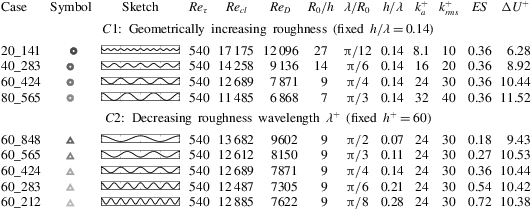
Cross-sectional sketch of the rough-wall pipe for a range of roughness heights and wavelengths. The thin grey line illustrates the surface at a streamwise offset of half a wavelength. The grey filled cross-sections are the cases which have been simulated at
 $Re_{\unicode[STIX]{x1D70F}}=540$
. Group
 $C1$
are the cases where the roughness elements are geometrically scaled and group
 $C2$
are the cases where only the wavelength of the roughness elements are varied while maintaining a constant roughness height.
4 Mean velocity profiles
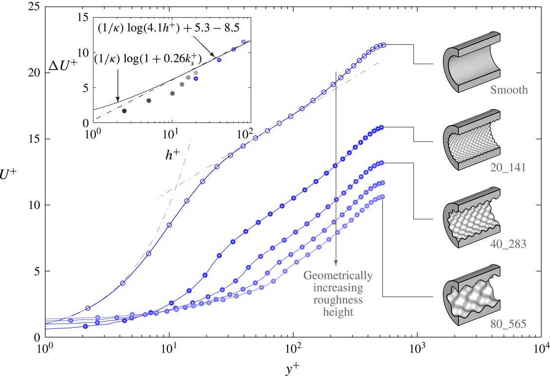
The mean velocity profiles for the geometrically scaled cases (
 $C1$
) are presented in figure 3. This figure is similar to the figure previously produced in Chan et al. (Reference Chan, MacDonald, Chung, Hutchins and Ooi2015) and is included here for ease of reference. The inset of figure 3 is the plot of the roughness function
 $\unicode[STIX]{x0394}U^{+}$
against
 $h^{+}$
.
 $\unicode[STIX]{x0394}U^{+}$
is calculated 300 viscous units above the crest of the roughness where the velocity profiles of both the smooth and rough cases are self-similar. As expected, increments of
 $h^{+}$
corresponds to an increase in
 $\unicode[STIX]{x0394}U^{+}$
. For
 $h^{+}\geqslant 60$
, it appears that
 $\unicode[STIX]{x0394}U^{+}$
increases logarithmically with
 $h^{+}$
, thereby indicating that the flow is approaching the fully rough regime. In addition, the wall shear stress for case 60_424 is mostly form/pressure drag (75 % of total drag due to pressure drag) as one would expect for this surface in the fully rough regime (Chan et al.
Reference Chan, MacDonald, Chung, Hutchins and Ooi2014). The roughness function for this roughness exhibits the inflectional type behaviour previously observed of sandgrain type roughness and approaches the fully rough asymptote from below. This roughness is in the region where the roughness function is independent of the effective slope
 $ES=0.36>0.35$
(Schultz & Flack Reference Schultz and Flack2009) and has an equivalent sandgrain roughness height of
 $k_{s}=4.1h$
(Chan et al.
Reference Chan, MacDonald, Chung, Hutchins and Ooi2015). Wavy surfaces on the other hand (
 $ES<0.35$
), such as those synthetically created by Barros, Schultz & Flack (Reference Barros, Schultz and Flack2017), are found to exhibit a Colebrook type roughness function where the roughness function profile reaches the fully rough asymptote from above.
Streamwise velocity profile for the geometrically increasing roughness cases (group
 $C1$
). Dash-dotted lines show
 $U^{+}=y^{+}$
and
 $U^{+}=(1/\unicode[STIX]{x1D705})\log (y^{+})+C$
,
 $\unicode[STIX]{x1D705}=0.40$
and
 $C=5.3$
. Inset: roughness function
 $\unicode[STIX]{x0394}U^{+}$
against roughness semi-amplitude
 $h^{+}$
. The solid circles are from the simulations of Chan et al. (Reference Chan, MacDonald, Chung, Hutchins and Ooi2015) at
 $Re_{\unicode[STIX]{x1D70F}}=180$
. Dash-dotted line of the inset flow demarcates the fully rough asymptote where
 $k_{s}^{+}=4.1h^{+}$
and the solid line represents Colebrook ‘universal’ roughness function (Colebrook Reference Colebrook1939).

Streamwise velocity profile for the increasing roughness wavelength cases (group
 $C2$
). Dash-dotted lines show
 $U^{+}=y^{+}$
and
 $U^{+}=(1/\unicode[STIX]{x1D705})\log (y^{+})+C$
,
 $\unicode[STIX]{x1D705}=0.40$
and
 $C=5.3$
. Dashed vertical line shows the wall-normal location of the crest of the roughness. Inset: roughness function
 $\unicode[STIX]{x0394}U^{+}$
against effective slope
 $ES$
. The red arrows illustrates the predicted trend when
 $ES\rightarrow 0$
and
 $ES\rightarrow \infty$
.

The mean velocity profiles for group
 $C2$
are plotted in figure 4. Case 60_424 which has
 $ES=0.36$
is in the fully rough regime. Therefore, it can be inferred that cases 60_283 and 60_212 with
 $ES>0.36$
are also close to the fully rough regime (since they have similar values of
 $\unicode[STIX]{x0394}U^{+}$
). Decreasing the wavelength of the roughness while maintaining the height of the roughness increases the
 $ES$
(or solidity) of the surface. Initially,
 $\unicode[STIX]{x0394}U^{+}$
increases steeply with increasing
 $ES$
but then plateaus (inset of figure 4). It is expected that at the limits, as
 $ES\rightarrow 0$
, the surface will approach a smooth wall and
 $\unicode[STIX]{x0394}U^{+}$
will be zero. On the other hand, as
 $ES\rightarrow \infty$
the velocity at the crest of the roughness approaches zero and becomes a smooth wall with a wall-normal offset equivalent to the roughness height (MacDonald et al.
Reference MacDonald, Chan, Chung, Hutchins and Ooi2016). Case 60_212 is entering the dense regime, where
 $\unicode[STIX]{x0394}U^{+}$
will start to decrease with increasing
 $ES$
or solidity (Jiménez Reference Jiménez2004). However, in truth 60_212 is very close to the solidity which yields a peak
 $\unicode[STIX]{x0394}U^{+}$
, and much larger increases in
 $ES$
than those simulated here would be required before one sees a noticeable drop in
 $\unicode[STIX]{x0394}U^{+}$
(refer to MacDonald et al. (Reference MacDonald, Chan, Chung, Hutchins and Ooi2016)). Nonetheless, the centreline Reynolds number and bulk Reynolds number for this particular case have also increased compared to case 60_283 (refer to table 2, which again confirms a slight reduction in
 $C_{f}$
).
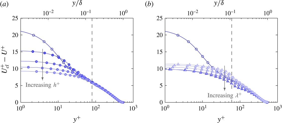
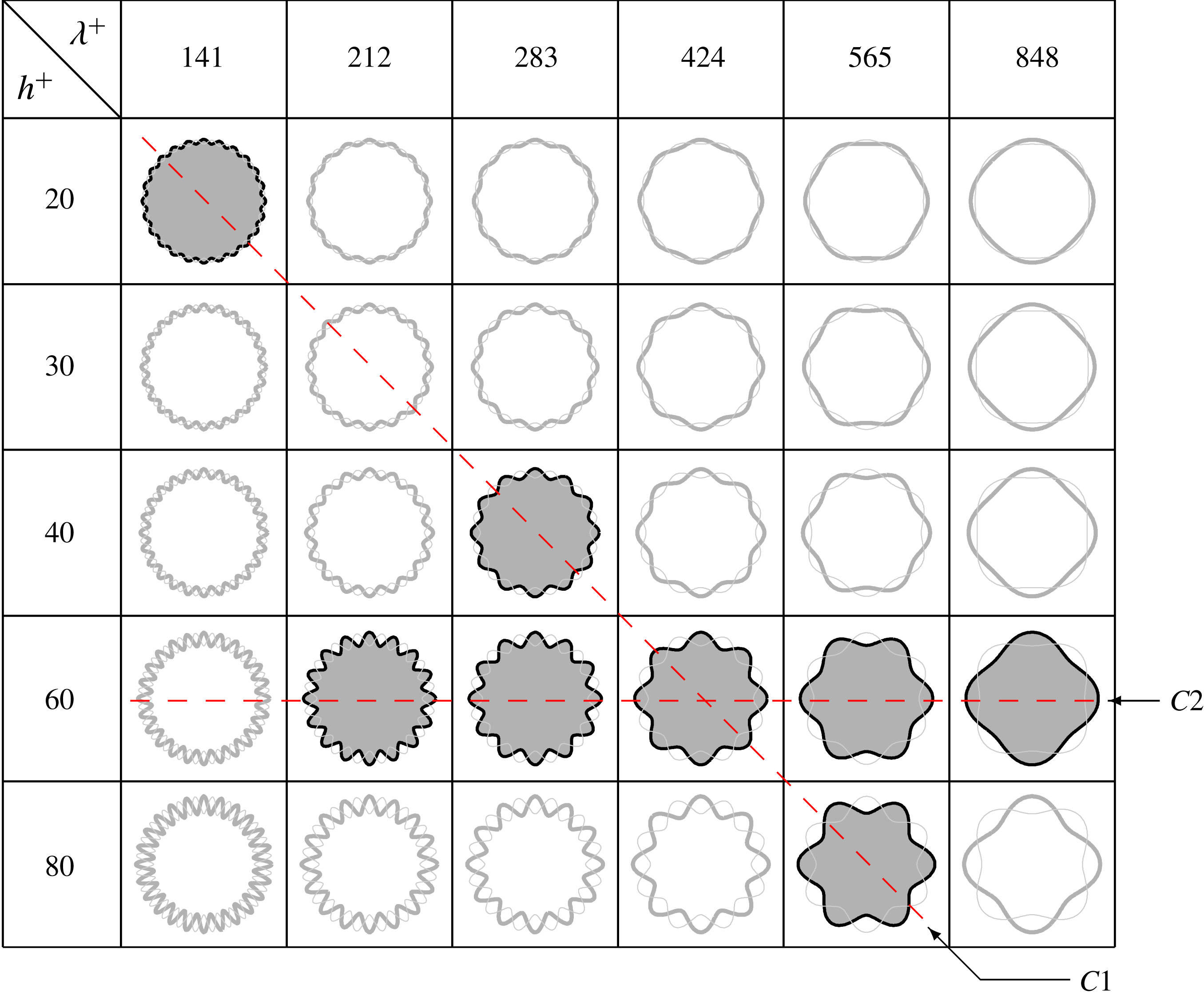
Plotting the velocity defect in figure 5, we observe that the profiles for group
 $C2$
(figure 5
b) are self-similar only when
 $y^{+}\geqslant 200$
. The notable outliers are cases 60_212 and 60_283 which have a relatively high solidity of
 $\unicode[STIX]{x1D6EC}=0.27$
and
 $0.36$
respectively (or
 $ES=0.54$
and
 $0.72$
). It is possible that the closely packed roughness has shifted the virtual origin of the wall closer to the crest of the roughness (MacDonald et al.
Reference MacDonald, Chan, Chung, Hutchins and Ooi2016). Current simulations are especially sensitive to the location of the virtual origin due to the large blockage ratio of the pipe
 $h/R_{0}$
. Another outlier is case 60_848 due to the occurrence of large secondary flows (as will be discussed in § 9). The previous study by Chan et al. (Reference Chan, MacDonald, Chung, Hutchins and Ooi2015) found that the velocity defect for the roughness group
 $C2$
in the transitionally rough regime (
 $h^{+}\leqslant 20$
) agrees well even in the vicinity of the roughness due to the much weaker secondary flow. The velocity defect profiles for group
 $C1$
(figure 5
a) are self-similar from approximately 20 viscous units above the crest of the roughness.
Velocity defect for groups (a)
 $C1$
and (b)
 $C2$
. Dashed vertical line shows the wall-normal location of the crest of the largest roughness in the group (
 $y^{+}=h^{+}$
).
5 Triple decomposition
A turbulent quantity can be decomposed into its mean and fluctuating component
 $$\begin{eqnarray}u_{i}(r,\unicode[STIX]{x1D703},x,t)=\overline{u}_{i}(r,\unicode[STIX]{x1D703},x)+u_{i}^{\prime \prime }(r,\unicode[STIX]{x1D703},x,t),\end{eqnarray}$$
where
 $\overline{u}_{i}$
is the time-averaged mean (where
 $\overline{\phantom{u}}$
denotes temporal averaging) and
 $u_{i}^{\prime \prime }$
is the fluctuation about the time-averaged mean (which is also known as the turbulent fluctuation) in the
 $i$
direction. This decomposition is known as the Reynolds decomposition. However, in a rough-wall flow, variations due to the unevenness of the spatial geometry must be taken into account when analysing the turbulent flow data. Therefore, a triple decomposition is applied to the turbulent quantity where it is decomposed into three components (Reynolds & Hussain Reference Reynolds and Hussain1972; Coceal & Belcher Reference Coceal and Belcher2004),
 $$\begin{eqnarray}u_{i}(r,\unicode[STIX]{x1D703},x,t)=U_{i}(r)+\tilde{u} _{i}(r,\unicode[STIX]{x1D703},x)+u_{i}^{\prime \prime }(r,\unicode[STIX]{x1D703},x,t).\end{eqnarray}$$
Here,
 $U_{i}=\langle \overline{u_{i}}\rangle$
is the spatial (
 $\langle \;\rangle$
denote in fluid spatial averaging) and temporally averaged mean, which is also known as the global mean and
 $\tilde{u} _{i}=\overline{u}_{i}-U_{i}$
is the spatial variation of the time-averaged flow around individual roughness elements which is defined as the coherent or dispersive component. The coherent fluctuation
 $\tilde{u} _{i}$
arises due to the unevenness of a surface and is only a function of the spatial coordinates. The sum of
 $\tilde{u} _{i}+u_{i}^{\prime \prime }=u_{i}^{\prime }$
is the fluctuation about the global (temporally and spatially averaged) mean which contains both the turbulent and coherent fluctuations. This quantity will be referred to as the total fluctuation. For a smooth wall,
 $\tilde{u} _{i}=0$
and therefore
 $u_{i}^{\prime }=u_{i}^{\prime \prime }$
. The triple decomposition is a result of double averaging, where the governing equations are averaged over time and then in space. This technique has been used to analyse plant canopy flows (Raupach & Shaw Reference Raupach and Shaw1982; Finnigan Reference Finnigan1985, Reference Finnigan2000) and also in open-channel flow over rough beds (Nikora et al.
Reference Nikora, Goring, McEwan and Griffiths2001, Reference Nikora, McEwan, McLean, Coleman, Pokrajac and Walters2007; Mignot, Barthelemy & Hurther Reference Mignot, Barthelemy and Hurther2009) where the rough surfaces are spatially inhomogeneous. These different fluctuating components will be used to analyse the turbulent features of the flow.
The premultiplied energy spectrum is an important tool which can be used to determine the dominant wavelengths of the turbulent structures in the flow. To calculate the spatial premultiplied energy spectrum, the Cartesian ‘O-grid’ has to be mapped to a cylindrical–polar grid where the grids are equally spaced in the azimuthal direction. A third-order cubic polynomial interpolation is used and the cylindrical–polar grid is mapped to the Cartesian grid as closely as possible to minimise the interpolation error. The largest error occurs at the centre of the pipe where there are only a few cells in the azimuthal direction. To calculate the energy spectrum within the roughness canopy, the area occupied by the roughness is zero padded. While this physically models the flow (velocity within the solid is zero), the zero padding reduces the value of
 $u_{rms}^{\prime \prime +}$
(root-mean-square fluctuations) when calculated from the spectrum. This difference becomes more prominent further within the roughness canopy and therefore one has to be careful when interpreting the results in this region. Above the crest of the roughness, the
 $u_{rms}^{\prime \prime +}$
values calculated from the premultiplied energy spectra agree well with the raw profiles (
 ${\leqslant}\pm 1\,\%$
difference for all three velocity components) therefore indicating that the interpolation has not significantly filtered the data.
Contours of the streamwise premultiplied energy spectrum for the streamwise velocity (a) total fluctuation
 $k_{x}E_{u_{x}^{\prime }u_{x}^{\prime }}^{+}$
, (c) coherent fluctuation
 $k_{x}E_{\tilde{u} _{x}\tilde{u} _{x}}^{+}$
and (e) turbulent fluctuation
 $k_{x}E_{u_{x}^{\prime \prime }u_{x}^{\prime \prime }}^{+}$
for case 20_141 and (g) for the smooth-wall case with contour levels of 0.25, 0.5 with subsequent 0.5 intervals. The smooth-wall case (thin black lines) is also plotted in (a) and (e) for reference. Horizontal and vertical black dashed line corresponds to the wavelength and the crest of the roughness elements (
 $y=h$
); ○ and
 $+$
symbols denote the peak in the contour for the smooth and rough cases respectively. Contours of the instantaneous streamwise velocity at
 $y^{+}\approx 20$
are plotted in (b,d,f,h) for the corresponding fluctuating terms. Inset contour shows a close-up view of the rectangular region and the flow is from left to right.
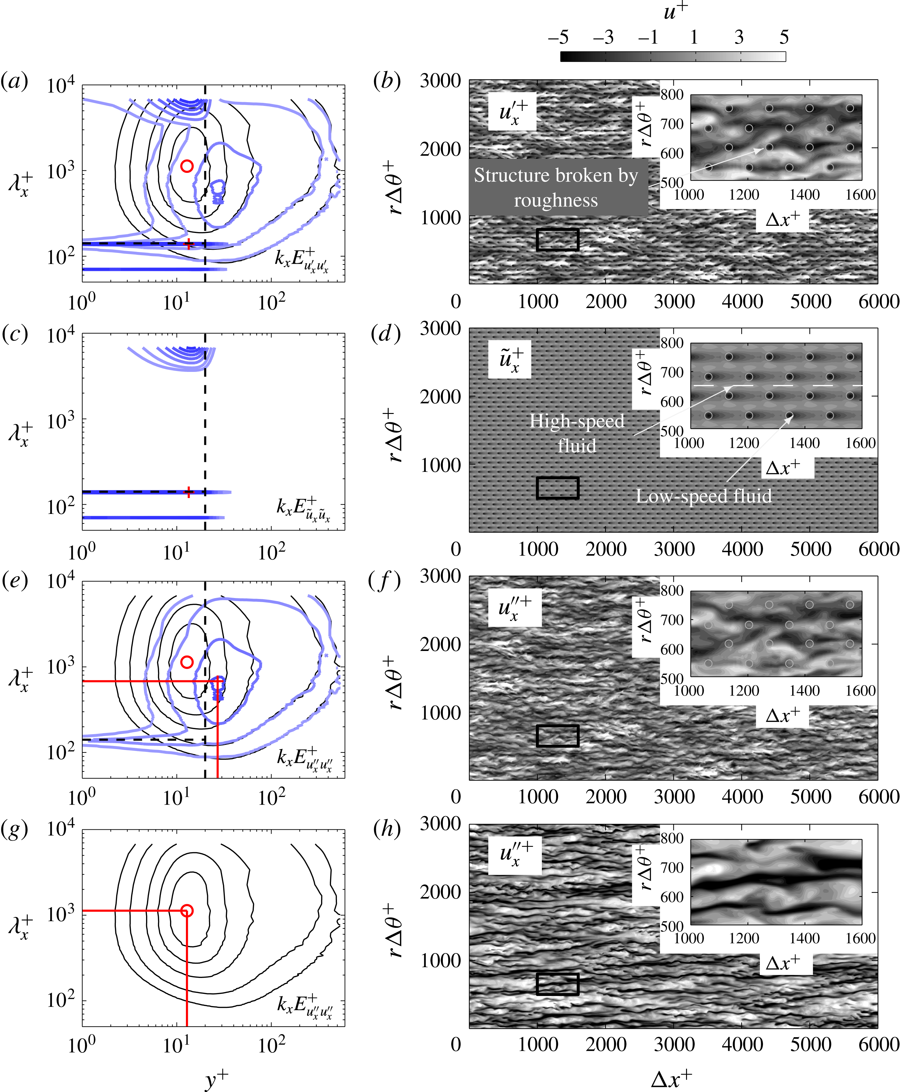
Figure 6 shows the streamwise premultiplied energy spectrum of the streamwise velocity (a) total fluctuation
 $k_{x}E_{u_{x}^{\prime }u_{x}^{\prime }}^{+}$
, (c) coherent fluctuation
 $k_{x}E_{\tilde{u} _{x}\tilde{u} _{x}}^{+}$
and (e) turbulent fluctuation
 $k_{x}E_{u_{x}^{\prime \prime }u_{x}^{\prime \prime }}^{+}$
for case 20_141. In the contours of
 $k_{x}E_{u_{x}^{\prime }u_{x}^{\prime }}^{+}$
in figure 6(a), we observe that large amounts of energy are concentrated at the wavelength corresponding to the length of the pipe and at wavelengths corresponding to the roughness wavelength and its harmonics. These peaks in energy are dominated by the coherent fluctuations as clearly observed in the contours of
 $k_{x}E_{\tilde{u} _{x}\tilde{u} _{x}}^{+}$
in figure 6(c). The coherent fluctuations are independent of time and only depend on the spatial topology of the roughness. For this particular sinusoidal roughness, high-speed fluid resides between the roughness elements which is the path of least resistance (see figure 6
d). These regions of high-speed fluid are infinitely long and correspond to the peak in the premultiplied energy spectrum at
 $\unicode[STIX]{x1D706}_{x}^{+}=L_{x}^{+}$
. The distinct peaks at the wavelength correlating to the wavelength of the roughness elements are due to the low-speed fluid in the wake of the roughness.
Removing the coherent fluctuations from the total fluctuations, we obtain the turbulent fluctuation of the fluid. Now, when plotting the contours of
 $k_{x}E_{u_{x}^{\prime \prime }u_{x}^{\prime \prime }}^{+}$
in figure 6(e), the spikes of energy are mostly removed but with clear remaining concentration at the roughness wavelength. While the coherent fluctuation is dominant within the roughness canopy and quickly reduces to zero at approximately 20 viscous units above the crest of the roughness elements (figure 6
c), energy of the turbulent fluctuation is redistributed to shorter streamwise lengths as compared to the smooth wall (shown as solid black lines) up to wall-normal height
 $y^{+}\approx 300$
for this particular roughness case (see figure 6
e). The inner peak of the contours of the streamwise premultiplied energy spectrum indicates that the near-wall cycle may still exist for this particular case which is in the transitionally rough regime. The inner peak is located at a higher wall-normal location and at a reduced streamwise length,
 $\unicode[STIX]{x1D706}_{x}^{+}\approx 681$
at
 $y^{+}\approx 27$
compared to the smooth-wall case where
 $\unicode[STIX]{x1D706}_{x}^{+}\approx 1100$
at
 $y^{+}\approx 13$
in figure 6(g). The peak energy is also significantly reduced, suggesting that, if it is still associated with the classical near-wall cycle, the cycle will have been substantially weakened.
Contours of total fluctuations
 $u_{x}^{\prime +}$
at radial location of
 $y^{+}\approx 20$
in figure 6(b) show the high-speed streaks being broken up by the roughness elements which are constricting the streamwise and spanwise size of these structures. The behaviour can be contrasted to the smooth-wall fluctuations at the same Reynolds number and
 $y^{+}$
as shown in figure 6(h). Plotting the contours of turbulent fluctuation
 $u_{x}^{\prime \prime +}$
in figure 6(f), the streaky high- and low-speed structures appear to still exist and are nominally similar to the structures observed in a smooth wall at the same wall-normal height in figure 6(h) although with slightly smaller streamwise length and less energy.
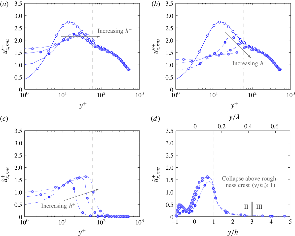
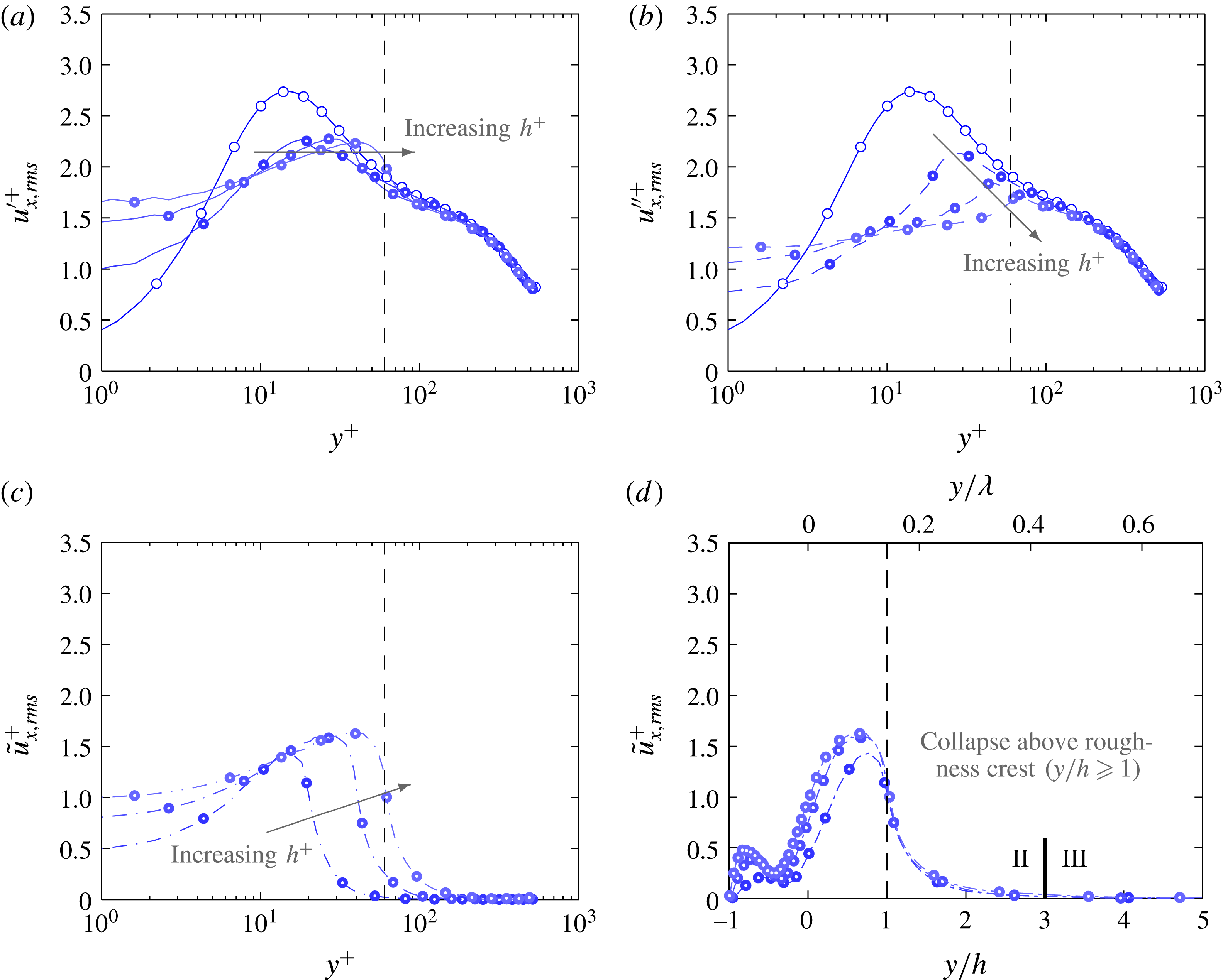
Streamwise velocity stress for group
 $C1$
due to (a) total fluctuation (solid lines), (b) turbulent fluctuation (dash lines) and (c) coherent fluctuation (dash-dotted lines) plotted against viscous wall-normal height and (d) wall-normal height normalised by roughness semi-amplitude. Dashed vertical line shows the wall-normal location of the crest of the largest roughness in the group (
 $y^{+}=h^{+}$
) and the solid vertical line in (d) demarcates the roughness sublayer (II) and the outer layer (III).
6 Stress profiles
The streamwise velocity stress profiles for
 $u_{x,rms}^{\prime +}$
,
 $u_{x,rms}^{\prime \prime +}$
and
 $\tilde{u} _{x,rms}^{+}$
for cases 20_141, 40_283 and 60_424 in group
 $C1$
are plotted in figure 7. With increasing roughness height, the location of maximum
 $u_{x,rms}^{\prime +}$
and
 $u_{x,rms}^{\prime \prime +}$
in figures 7(a) and 7(b) gets pushed to higher wall-normal heights and occur close to the crest of the roughness. The maximum value of the turbulent fluctuations
 $u_{x,rms}^{\prime \prime +}$
decreases with increasing
 $h^{+}$
whereas the maximum value of the coherent stress
 $\tilde{u} _{x,rms}^{+}$
in figure 7(c) marginally increases with increasing
 $h^{+}$
. Plotting
 $\tilde{u} _{x,rms}^{+}$
against the wall-normal height normalised by roughness semi-amplitude (
 $y/h$
) in figure 7(d), a good collapse is observed above the crest of the roughness for all of the cases in group
 $C1$
, regardless of whether the roughness is in the transitionally rough or fully rough regime. These roughness cases have constant
 $h/\unicode[STIX]{x1D706}$
ratio and therefore normalising the wall-normal height with the wavelength of the roughness (
 $y/\unicode[STIX]{x1D706}$
) would also lead to the same collapse. Maximum
 $\tilde{u} _{x,rms}^{+}$
located within the roughness canopy is associated with large velocity variation of the time-averaged flow as the flow is channelled between the roughness elements. Above the crest of the roughness, the profile decreases drastically and when
 $y/h\gtrsim 3$
(
 $y/\unicode[STIX]{x1D706}\gtrsim 0.43$
),
 $\tilde{u} _{x,rms}^{+}$
is approximately zero (less than 3.6 % of the value at
 $y/h=1$
).
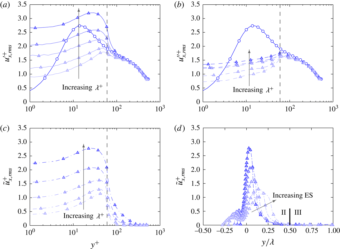
Streamwise velocity stress for group
 $C2$
due to (a) total fluctuation (solid lines), (b) turbulent fluctuation (dash lines) and (c) coherent fluctuation (dash-dotted lines) plotted against viscous wall-normal height and (d) wall-normal height normalised by roughness wavelength. Dashed vertical line shows the wall-normal location of the crest of the roughness in the group (
 $y^{+}=h^{+}$
) and the solid vertical line in (d) demarcates the roughness sublayer (II) and the outer layer (III).

The streamwise velocity stress profiles for
 $u_{x,rms}^{\prime +}$
,
 $u_{x,rms}^{\prime \prime +}$
and
 $\tilde{u} _{x,rms}^{+}$
for group
 $C2$
are plotted in figure 8. The peak of the total fluctuation
 $u_{x,rms}^{\prime +}$
in figure 8(a) increases as the wavelength of the roughness increases. This increase is also observed by Chau & Bhaganagar (Reference Chau and Bhaganagar2012) who found that the peak of the streamwise velocity fluctuation increases with decreasing
 $h/\unicode[STIX]{x1D706}$
ratio for their irregular roughness. However, looking at the plot of the turbulent fluctuations
 $u_{x,rms}^{\prime \prime +}$
in figure 8(b), the magnitude of the peak does not increase significantly with increasing roughness wavelength. Rather, the large increase in
 $u_{x,rms}^{\prime +}$
is due to the rise in the coherent component of the velocity fluctuation
 $\tilde{u} _{x,rms}^{+}$
(figure 8
c), which occurs because of the channelling of the flow around the roughness within the roughness canopy. Plotting
 $\tilde{u} _{x,rms}^{+}$
against
 $y/\unicode[STIX]{x1D706}$
in figure 8(d), reasonable collapse of the profiles is observed for
 $y/\unicode[STIX]{x1D706}\geqslant 0.25$
. Cases 60_283 and 60_212 are again outliers (previously observed in the velocity defect plot in figure 5
b) as the virtual origin of the wall has shifted to a higher wall-normal location. Selecting the virtual origin to be the location where
 $U^{+}=2$
(instead of
 $R_{0}$
) leads to a convincing collapse for the cases in group
 $C2$
(not shown in current manuscript).
 $\tilde{u} _{x,rms}^{+}$
reduces to approximately zero at wall-normal heights
 $y/\unicode[STIX]{x1D706}\gtrsim 0.5$
.
Wall-normal velocity stress due to (a,b) total fluctuation and (c,d) coherent fluctuation for groups (a,c)
 $C1$
and (b,d)
 $C2$
. Vertical dashed line shows the wall-normal location of the crest of the largest roughness in the group (
 $y=h$
). Region I (grey shade)- roughness canopy, region II (blue shade)- roughness sublayer, region III- outer layer. The solid vertical line in (d) demarcates the roughness sublayer (II) and the outer layer (III).
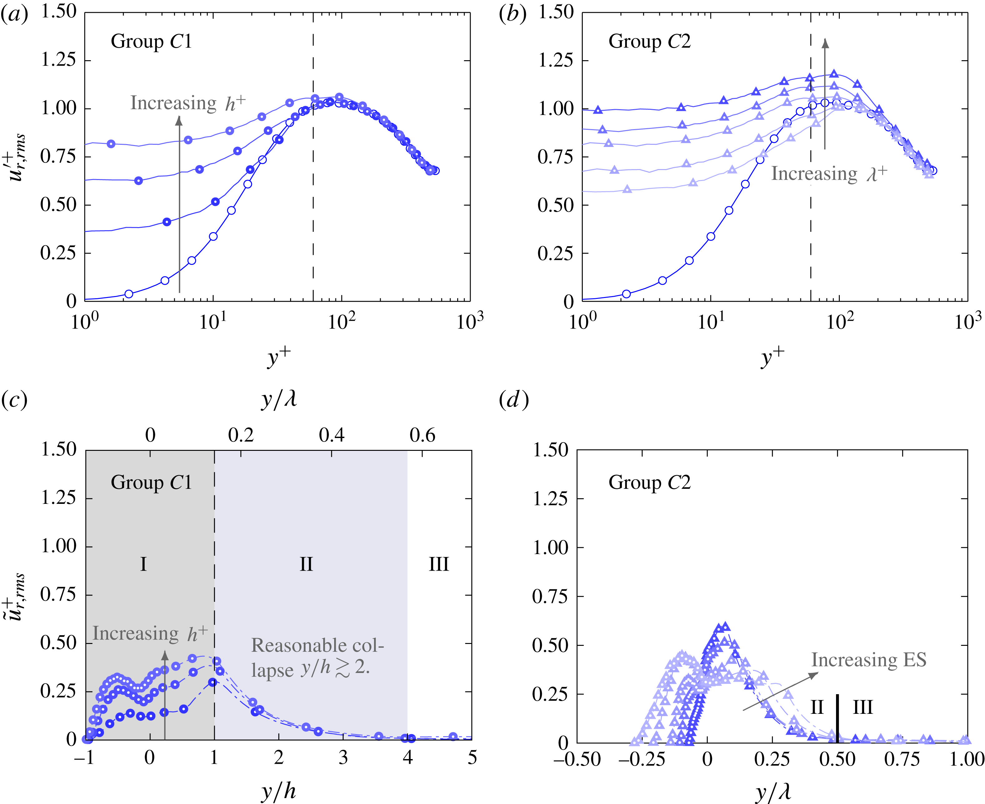
The radial velocity stress component due to the total fluctuation
 $u_{r,rms}^{\prime +}$
and coherent fluctuation
 $\tilde{u} _{r,rms}^{+}$
for both groups
 $C1$
and
 $C2$
are plotted in figure 9. The wall-normal velocity fluctuations contribute to the turbulent mixing of low-speed fluid near the wall with the high-speed fluid in the outer region of the flow. For group
 $C2$
, the maximum
 $u_{r,rms}^{\prime +}$
increases with increasing roughness wavelength (figure 9
b). For case
 $C1$
, the maximum
 $u_{r,rms}^{\prime +}$
seems to be invariant with roughness height (figure 9
a), although there is height-dependent behaviour within the canopy. For both
 $C1$
and
 $C2$
, these profiles collapse on top of each other in the outer region of the flow (
 $y^{+}\geqslant 300$
).
Plotting the
 $\tilde{u} _{r,rms}^{+}$
profiles for group
 $C1$
, it is noticed that the maximum value occurs at the crest of the roughness and increases slightly with increments of roughness height (figure 9
c). Good collapse in the
 $\tilde{u} _{r,rms}^{+}$
profiles for group
 $C1$
is observed at
 $y/h\geqslant 2$
and falls to zero for
 $y/h\gtrsim 4$
or
 $y/\unicode[STIX]{x1D706}\gtrsim 0.57$
. This wall-normal location is slightly higher than that of the
 $\tilde{u} _{x,rms}^{+}$
profile in figure 7(d). The maximum value of
 $\tilde{u} _{r,rms}^{+}$
also increases slightly with increasing wavelength for group
 $C2$
(figure 9
d). Again, good collapse is observed in the
 $\tilde{u} _{r,rms}^{+}$
profiles for
 $y/\unicode[STIX]{x1D706}\geqslant 0.25$
(except for cases 60_283 and 60_212) and
 $\tilde{u} _{r,rms}^{+}$
reduces to zero when
 $y/\unicode[STIX]{x1D706}\gtrsim 0.5$
for all cases in group
 $C2$
. For case 60_848, this occurs at
 $y^{+}\approx 424$
which is in the outer layer of the flow. This again indicates that there are large stationary features present in the flow.
From these observations we can define three distinct regions in the turbulent flow over rough walls (see figure 9
c). The first region where
 $-1\leqslant y/h\leqslant 1$
, is (I) the roughness canopy where the fluid resides within the roughness elements. In this region, the contribution of the dispersive stresses is significant. Above the roughness canopy is (II) the roughness sublayer, where the effects of the roughness are felt by the turbulent fluid. When considering the second-order statistics, simulations of group
 $C1$
and
 $C2$
indicate that the roughness sublayer scales with the roughness wavelength and extends up to
 $y/\unicode[STIX]{x1D706}\approx 0.5$
where
 $\tilde{u} _{x}^{+}$
and
 $\tilde{u} _{r}^{+}$
are approximately zero. Region (III) is the area where the turbulent statistics are independent of the influence of the roughness and collapses to the equivalent smooth-wall case. The good collapse in the
 $u_{x,rms}^{\prime \prime +}$
and
 $u_{r,rms}^{\prime \prime +}$
profiles in the outer region of the flow indicates support for Townsend’s outer-layer hypothesis. However, it is important to highlight that the Reynolds number of the flow (
 $540<Re_{\unicode[STIX]{x1D70F}}<667$
) is insufficient to discern between the near-wall inner scales and the log region outer scales (Hutchins & Marusic Reference Hutchins and Marusic2007). Therefore, the term ‘outer layer’ in the current context is used to define the region where the flow statistics of the rough wall are similar to the smooth wall (in the spirit of Townsend’s outer-layer similarity argument for rough walls (Townsend Reference Townsend1976)).
7 One-dimensional premultiplied energy spectra
The contours of the streamwise and spanwise premultiplied energy spectra for the streamwise velocity turbulent fluctuation (
 $k_{x}E_{u_{x}^{\prime \prime }u_{x}^{\prime \prime }}^{+}$
and
 $k_{s}E_{u_{x}^{\prime \prime }u_{x}^{\prime \prime }}^{+}$
) for selected cases in groups
 $C1$
and
 $C2$
are plotted in figures 10 and 11 respectively. When calculating the spanwise premultiplied energy spectrum in a pipe, the spanwise length changes with radial location and causes energy to be concentrated at
 $\unicode[STIX]{x1D706}_{s}^{+}\rightarrow 0$
as
 $r\rightarrow 0$
. The grey shaded region is the roughness canopy defined as
 $-h<y<h$
. When considering the contours of
 $k_{x}E_{u_{x}^{\prime \prime }u_{x}^{\prime \prime }}^{+}$
and
 $k_{s}E_{u_{x}^{\prime \prime }u_{x}^{\prime \prime }}^{+}$
, the roughness sublayer (blue shaded region) is defined as the region above the roughness canopy to the wall-normal height where the contours of the rough-wall spectrum begin to coincide with the smooth wall. This definition which demands similarity in turbulent structure will yield a roughness sublayer that extends further from the wall than definitions based on root-mean-squared quantities.
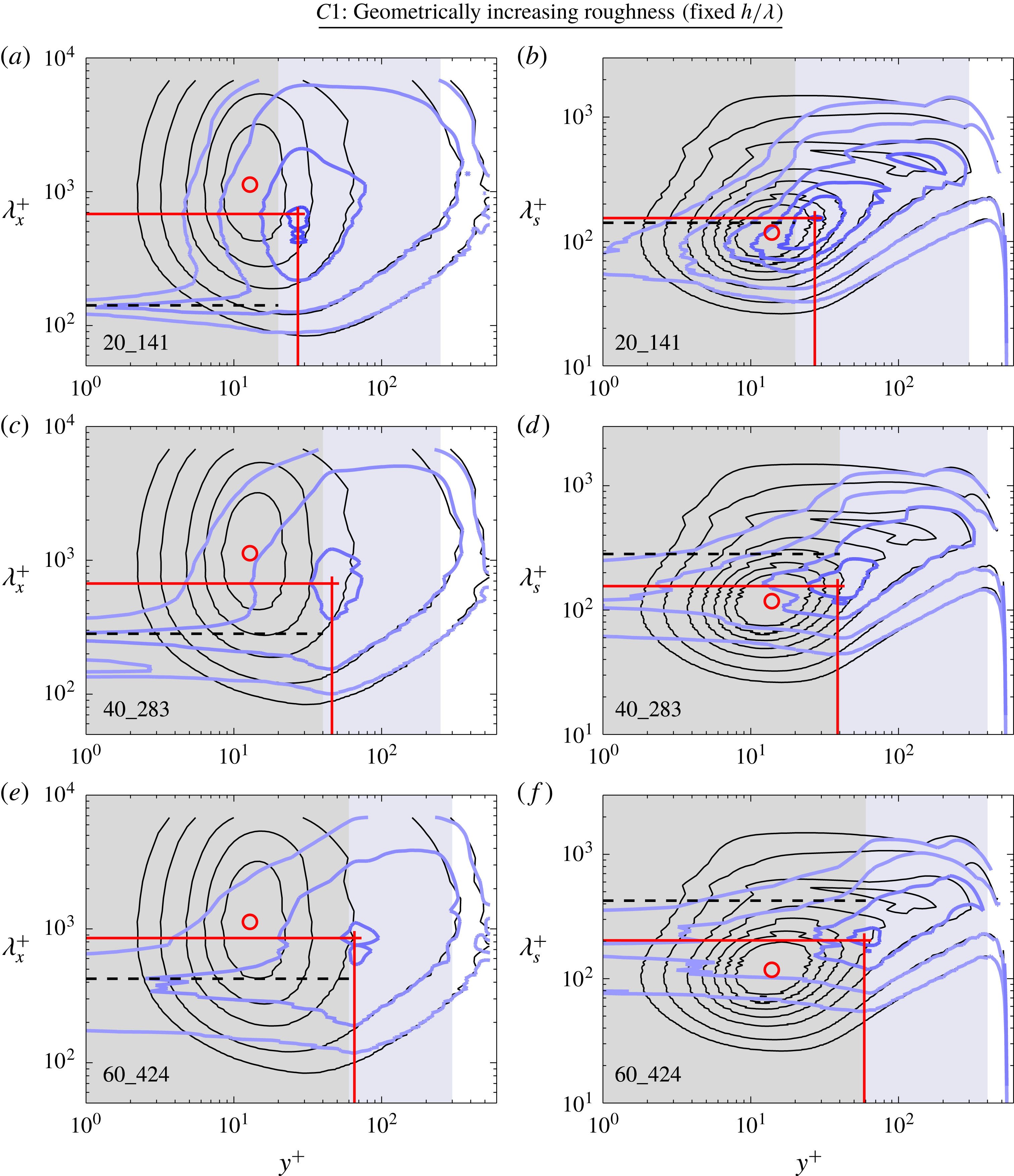
Contours of the (a,c,e) streamwise and (b,d,f) spanwise premultiplied energy spectra of the streamwise velocity turbulent fluctuation (
 $k_{x}E_{u_{x}^{\prime \prime }u_{x}^{\prime \prime }}^{+}$
and
 $k_{s}E_{u_{x}^{\prime \prime }u_{x}^{\prime \prime }}^{+}$
) for group
 $C1$
. Blue contour lines represent the rough case and thin black lines represent the smooth case. Contour levels start at 0.25, 0.5 with subsequent 0.5 intervals. ○ and
 $+$
symbols denote the peak in the contour for the smooth and rough cases respectively. Horizontal dashed line corresponds to the wavelength of the roughness elements. The grey, blue and white regions represent the roughness canopy, roughness sublayer and outer layer of the flow.
Contours of the (a,c,e) streamwise and (b,d,f) spanwise premultiplied energy spectra of the streamwise velocity turbulent fluctuation (
 $k_{x}E_{u_{x}^{\prime \prime }u_{x}^{\prime \prime }}^{+}$
and
 $k_{s}E_{u_{x}^{\prime \prime }u_{x}^{\prime \prime }}^{+}$
) for group
 $C2$
. Blue contour lines represent the rough case and thin black lines represent the smooth case. Contour levels start at 0.25, 0.5 with subsequent 0.5 intervals. ○ and
 $+$
symbols denote the peak in the contour for the smooth and rough cases respectively. Horizontal dashed line corresponds to the wavelength of the roughness elements. The grey, blue and white regions represent the roughness canopy, roughness sublayer and outer layer of the flow.
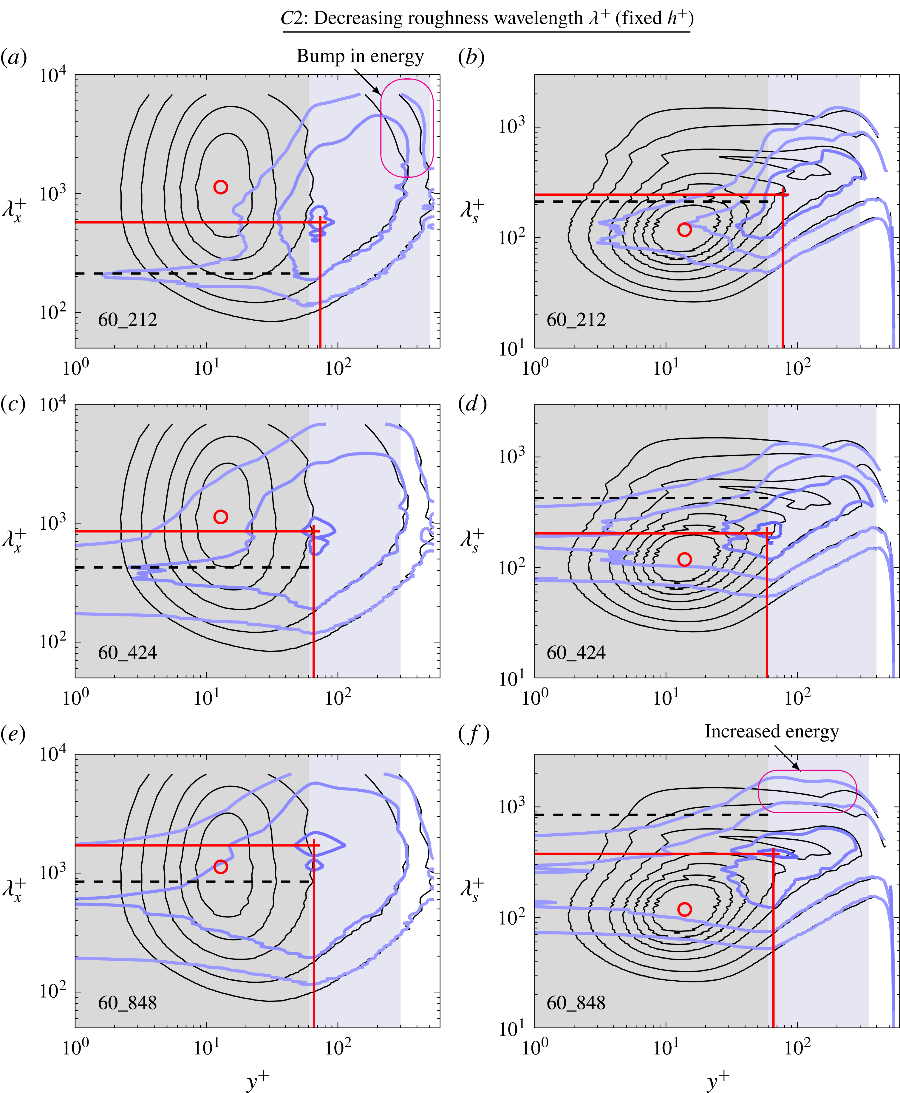
Energy within the roughness canopy in the streamwise premultiplied energy spectra is concentrated at wavelengths corresponding to the roughness wavelength (shown by the black dashed line) and the energy within the roughness canopy in the spanwise premultiplied energy spectra is concentrated at wavelengths half of the roughness wavelength as the flow is spatially confined (recall that we are zero padding the interpolated fields within the solid roughness).
With increasing roughness height (group
 $C1$
), the magnitude of the peaks of
 $k_{x}E_{u_{x}^{\prime \prime }u_{x}^{\prime \prime }}^{+}$
and
 $k_{s}E_{u_{x}^{\prime \prime }u_{x}^{\prime \prime }}^{+}$
in figure 10 decreases (as also observed in the profiles
 $u_{x,rms}^{\prime \prime +}$
in figure 7
b). For case 60_424 which is in the fully rough regime, the near-wall region which in a smooth wall is occupied by the near-wall cycle, is completely replaced by the flow within the roughness canopy. Therefore, for cases in the fully rough regime, the peak in the contour of
 $k_{x}E_{u_{x}^{\prime \prime }u_{x}^{\prime \prime }}^{+}$
does not necessarily represent the canonical near-wall cycle. The streamwise wavelength of the peak in case 60_424 is higher compared to case 40_283 (figure 10
c,e) and appears to scale with the roughness wavelength as the flow approaches the fully rough regime. The spanwise wavelength of the peak also increases albeit marginally from
 $\unicode[STIX]{x1D706}_{s}^{+}\approx 154$
for case 20_141 to
 $\unicode[STIX]{x1D706}_{s}^{+}\approx 203$
for case 60_424.
For group
 $C2$
, we observe that the peak energy in the streamwise direction (figure 11
a,c,e) is redistributed depending on the wavelength of the roughness elements. There is a bump in the contours of
 $k_{x}E_{u_{x}^{\prime \prime }u_{x}^{\prime \prime }}^{+}$
in the outer region for case 60_212 (figure 11
a) and the contour does not coincide with the contours of the smooth wall. This is possibly due to the high blockage ratio of the pipe as it approaches the dense regime. This difference in the redistribution of energy is not observed in the profile of
 $u_{x,rms}^{\prime \prime +}$
in figure 8(b) which agrees well with the other smooth and rough cases in the outer region of the flow. The spanwise wavelength of the peak energy for cases 60_848 occurs at
 $\unicode[STIX]{x1D706}_{s}^{+}\approx 376$
which is significantly higher than the other cases (figure 11
f). An increase in the energy contribution of the largest spanwise wavelength in the roughness sublayer is also observed for this particular case due to the occurrence of large secondary flows.
Overall, roughness decreases the energy contained in the larger-scale structures in the streamwise direction throughout most of the domain (up to
 $y^{+}\approx 300$
). The rough-wall contours of
 $k_{x}E_{u_{x}^{\prime \prime }u_{x}^{\prime \prime }}^{+}$
and
 $k_{s}E_{u_{x}^{\prime \prime }u_{x}^{\prime \prime }}^{+}$
collapse to the smooth-wall contours at a much higher wall-normal height compared to the first- and second-order statistics. Therefore, a larger roughness sublayer is obtained when considering the one-dimensional premultiplied energy spectrum, suggesting that subtle differences in the turbulent structures persist beyond where outer-layer similarity is observed in the first- and second-order statistics.
8 Instantaneous streamwise velocity contours
Figure 12 shows the contours of instantaneous streamwise turbulent fluctuation
 $u_{x}^{\prime \prime +}$
for the smooth and selected rough cases at
 $y^{+}\approx 30$
. The average streamwise and spanwise lengths of the structures are also plotted for reference. These average lengths are obtained from the maximum value of
 $k_{x}E_{u_{x}^{\prime \prime }u_{x}^{\prime \prime }}^{+}$
and
 $k_{s}E_{u_{x}^{\prime \prime }u_{x}^{\prime \prime }}^{+}$
at the particular wall-normal height. For case 20_141, this wall-normal height is 10 viscous units above the crest of the roughness and is located near the maximum value of
 $k_{x}E_{u_{x}^{\prime \prime }u_{x}^{\prime \prime }}^{+}$
. The low- and high-speed streaks in figure 12(b) are quite similar to the streaks observed in the smooth wall in figure 12(a) albeit being less intense and also having a shorter streamwise length, in line with the findings of MacDonald et al. (Reference MacDonald, Chan, Chung, Hutchins and Ooi2016) for roughness in the transitionally rough regime. At
 $y^{+}=30$
, the flow resides within the roughness canopy for cases 60_212 and 60_848. Interestingly, it appears that the structures are shorter in case 60_848 (figure 12
d) than case 60_212 (figure 12
c) where the roughness is more closely packed. There is also a noticeable increase in the spanwise length of these structures for case 60_848 as the flow has more space to meander around the roughness.
Contours of the instantaneous streamwise velocity turbulent fluctuation
 $u_{x}^{\prime \prime +}$
at
 $y^{+}\approx 30$
for the (a) smooth case, and rough cases (b) 20_141, (c) 60_212 and (d) 60_848. The horizontal and vertical solid red lines show the dominant streamwise and spanwise lengths of the structures obtained from the peak of the streamwise and spanwise premultiplied energy spectrum of the streamwise turbulent velocity at this wall-normal height.

Contours of the instantaneous streamwise velocity turbulent fluctuation
 $u_{x}^{\prime \prime +}$
at
 $y^{+}\approx 100$
for the (a) smooth case, and rough cases (b) 20_141, (c) 60_212 and (d) 60_848. The horizontal and vertical solid red lines show the dominant streamwise and spanwise lengths of the structures obtained from the peak of the streamwise and spanwise premultiplied energy spectrum of the streamwise turbulent velocity at this wall-normal height.

The contours of the
 $u_{x}^{\prime \prime +}$
at
 $y^{+}\approx 100$
are plotted in figure 13. For case 20_141, the energy from the largest structures is redistributed to the smaller wavelengths at this wall-normal height. However, it is difficult to distinguish the differences in the contours of
 $u_{x}^{\prime \prime +}$
between this rough-wall case (figure 13
b) with the smooth wall (figure 13
a) from qualitative comparison. The contours of
 $u_{x}^{\prime \prime +}$
for cases 60_212 and 60_848 in figures 13(c) and 13(d) are located at a wall-normal height close to the peak of
 $k_{x}E_{u_{x}^{\prime \prime }u_{x}^{\prime \prime }}^{+}$
. However, the high- and low-speed streaks observed do not resemble the streaks of the near-wall cycle as they are significantly wider. Rather, these structures better represent the large-scale structures which occur in the logarithmic region of the flow. There are distinct differences in the streamwise length of the structures for case 60_212 and 60_848 as they are greatly affected by the wavelength of the roughness (although again these differences are not immediately obvious from the instantaneous realisations).
9 Time-averaged velocity contours
Sketch of case 60_848 with isosurfaces of the time-averaged streamwise vorticity for one azimuthal roughness wavelength. The positive streamwise vorticity isosurface
 $\overline{\unicode[STIX]{x1D714}}_{x}^{+}=+0.01$
is coloured in red and the negative streamwise vorticity isosurface
 $\overline{\unicode[STIX]{x1D714}}_{x}^{+}=-0.01$
is coloured blue. Cross-sectional planes (a) I and (b) II show the contours of the time-averaged streamwise velocity
 $\overline{u}_{x}^{+}$
overlaid with line contours of
 $\overline{\unicode[STIX]{x1D714}}_{x}^{+}=\pm 0.01$
. Black arrows illustrates the transfer of low-speed fluid from the wall to the outer region of the flow and high-speed fluid from the outer region of the flow to the wall. (c) Cross-sectional sketch of the unwrapped rough-wall pipe. These counter rotating streamwise vortex pairs have a spacing of
 $l_{s}^{+}\approx 424$
. The white line shows the distribution of the time- and streamwise-averaged wall shear stress.

A sketch of the roughness geometry for case 60_848 is shown in figure 14. The tube-like surfaces coloured in red and blue are the isosurfaces of the positive and negative streamwise vorticity respectively. These alternating streamwise vortices indicate that there are secondary flows occurring above the roughness elements. Figure 14 also includes a closer look at the contours of the time-averaged streamwise velocity along cross-sectional plane I which is locally rough in the azimuthal direction (figure 14
a) and plane II which is locally smooth (figure 14
b). We observe regions of high-speed fluid residing along streamwise plane
 $B$
which is locally smooth in
 $x$
and low-speed fluid along streamwise plane
 $A$
which is locally rough in
 $x$
. The occurrence of these alternating low-momentum paths (LMPs) and high-momentum paths (HMPs) is due to the spanwise heterogeneity of the roughness which channels the flow. The red and blue contour lines are the positive and negative time-averaged streamwise vorticity (
 $\overline{\unicode[STIX]{x1D714}}_{x}^{+}=\pm 0.01$
). These secondary flows eject low-speed fluid from the wall to the outer region of the flow and transport high-speed fluid to the wall. This phenomenon can be explained simply by considering the mechanical energy balance where an imbalance in the local production and dissipation of turbulence gives rise to these secondary flows which assist in the transport of turbulent rich (poor) fluid to turbulent poor (rich) fluid (Hinze Reference Hinze1967; Anderson et al.
Reference Anderson, Barros, Christensen and Awasthi2015). The effects of these large secondary flows are clearly reflected in the streamwise and wall-normal velocity coherent stress profiles (figures 8
d and 9
d) which only reduce to zero in the outer region of the flow (
 $y^{+}\gtrsim 0.5\unicode[STIX]{x1D706}\approx 424$
). This roughness has an
 $ES$
of 0.18 which is similar to the pyramidal roughness of Schultz & Flack (Reference Schultz and Flack2009) which has an
 $ES$
of 0.19 and a shallow slope angle of 11
 $^{\circ }$
. They found that the roughness function for that wavy surface does not scale with the roughness height and this might due to the occurrence of large secondary flows which might be altering the outer layer of the flow.
Contours of the time-averaged streamwise velocity
 $\overline{u}_{x}^{+}$
overlaid with line contours of
 $\overline{\unicode[STIX]{x1D714}}_{x}^{+}=+0.01$
(red line) and
 $\overline{\unicode[STIX]{x1D714}}_{x}^{+}=-0.01$
(blue line) along plane I where the cross-section of the pipe is locally rough. The dashed black and white lines are at
 $y/\unicode[STIX]{x1D706}=0.5$
where the coherent stresses are zero. Flow is into the page.

The azimuthal variation of the mean wall shear stress (see figure 14
c) gives rise to these large-scale secondary motions. The variation of the wall shear stress for this three-dimensional sinusoidal roughness is periodic and has a wavelength half of the roughness wavelength
 $l_{s}=\unicode[STIX]{x1D706}_{s}/2$
. For case 60_848, the wavelength of the variation of these stresses is approximately equal to the boundary layer thickness (
 $l_{s}^{+}=424\approx \unicode[STIX]{x1D6FF}^{+}=540$
) which has been found to cause the development of large secondary flows that can penetrate the edge of the boundary layer (see § 1.1 of the introduction). These large secondary flows occurring in the pipe are similar to the secondary flows observed in duct flows (Brundrett & Baines Reference Brundrett and Baines1964). It is also worth mentioning that the square duct, when unwrapped/unrolled, becomes a straight inverted scalloped riblet with a fixed spanwise wavelength of
 $l_{s}=2\unicode[STIX]{x03C0}\unicode[STIX]{x1D6FF}/4$
. Therefore,
 $l_{s}/\unicode[STIX]{x1D6FF}=\unicode[STIX]{x03C0}/2$
, which is larger than 1, causes the occurrence of large secondary motions.
Secondary flows are also observed in the other roughness cases but reside mostly within the roughness canopy (see figure 15). It can be seen that the wall-normal and spanwise size of the secondary flows increases with increasing wavelength (figure 15
b,d,e,f). This is because the cases simulated here are in the intermediate state (
 $0.2\lesssim l_{s}/\unicode[STIX]{x1D6FF}\lesssim 2$
) where increments in the spanwise wavelength of the roughness results in a proportional increase in the size of the secondary flow (Yang & Anderson Reference Yang and Anderson2018). It is interesting that secondary flows are observed for this three-dimensional sinusoidal roughness where the roughness elements are staggered, which better represent a random roughness arrangement (Forooghi et al.
Reference Forooghi, Stroh, Magagnato, Jakirlić and Frohnapfel2017), whereas previous studies typically had streamwise aligned roughness (Goldstein & Tuan Reference Goldstein and Tuan1998; Vanderwel & Ganapathisubramani Reference Vanderwel and Ganapathisubramani2015; Medjnoun et al.
Reference Medjnoun, Vanderwel and Ganapathisubramani2018; Yang & Anderson Reference Yang and Anderson2018). It is important to note that the occurrence of these secondary flows is an artefact of the averaging of strong instantaneous turbulent events enhanced by the roughness (Kevin et al.
Reference Monty, Bai, Pathikonda, Nugroho, Barros, Christensen and Hutchins2017), hence in general they will not necessarily be obvious in instantaneous realisations.
10 Conclusion
DNS of a turbulent rough-wall pipe with a conforming grid was conducted at moderate Reynolds numbers where the height and wavelength of the three-dimensional sinusoidal roughness are systematically varied to enable a comprehensive investigation of secondary motion. The flow is simulated from the transitionally rough to the fully rough regime (group
 $C1$
) and from the wavy, sparse regime to the dense regime (group
 $C2$
). When analysing the statistics, the triple decomposition is used to separate the turbulent fluctuations from the coherent fluctuations which arise due to the roughness. The main findings of this paper can be summarised below:
(i) The coherent stress due to the coherent fluctuations is found to be dominant within the roughness canopy but quickly reduces above the crest of the roughness. Both simulations of groups
 $C1$
and
$C2$
have shown that the coherent stress depends on the roughness wavelength. For group
$C1$
, the coherent stress scales with the roughness height (and also the roughness wavelength as these cases are geometrically scaled) and approaches zero when
$y/h\gtrsim 4$
(
$y/\unicode[STIX]{x1D706}\gtrsim 0.57$
) both in the transitionally rough and fully rough regimes. For group
$C2$
, the coherent stress reduces to zero when
$y/\unicode[STIX]{x1D706}\gtrsim 0.5$
. This means that the lateral wavelength of a rough surface will likely influence our ability to observe outer-layer similarity over rough surfaces. Since the coherent stresses, which indicate the presence of secondary flows, extend up to
$y/\unicode[STIX]{x1D706}=0.5$
we would perhaps not expect to observe outer-layer similarity (or self-similar profiles) below this height. In cases where
$\unicode[STIX]{x1D706}\approx 2\unicode[STIX]{x1D6FF}$
(
$l_{s}\approx \unicode[STIX]{x1D6FF}$
) the coherent stresses (and secondary flows) would fill the entire boundary layer, and we would not expect to observe outer-layer similarity. This simple observation may provide some explanation for some of the discrepancy in the literature regarding outer-layer similarity over rough surfaces. Rather than focusing solely on
$\unicode[STIX]{x1D6FF}/k$
, the ratio
$\unicode[STIX]{x1D6FF}/l_{s}$
must also be considered.
(ii) Analysing the streamwise premultiplied energy spectra of the streamwise velocity turbulent fluctuation
$k_{x}E_{u_{x}^{\prime \prime }u_{x}^{\prime \prime }}^{+}$
, it is found that the energy contained in the larger structures are redistributed to shorter wavelengths even for the cases in the transitionally rough regime. This redistribution of energy extends up to
$y^{+}\approx 300$
, which is more than half of the outer-layer length scale of the pipe (
$y/\unicode[STIX]{x1D6FF}\approx 0.56$
). Results from the one-dimensional premultiplied energy spectra show a larger roughness sublayer than the mean velocity profile and second-order statistics. Higher-order statistics (unsurprisingly) present a more stringent interpretation on outer-layer similarity. It is possible that subtle structural modifications to turbulence over rough surfaces (compared to a smooth surface) may exist beyond heights where outer-layer collapse is observed in lower-order mean statistics.(iii) For the cases in the fully rough regime, the near-wall structures typically observed over a smooth wall are completely replaced by the flow within the roughness canopy for this particular roughness. The peak in the premultiplied energy spectra in the roughness sublayer (above the roughness crest) better represents the large-scale structures which occur in the logarithmic region of the flow.
(iv) Time-independent secondary flows are observed when analysing the time-averaged velocities. The size and wall-normal extent of these secondary flows scale with the spanwise roughness wavelength
$\unicode[STIX]{x1D706}_{s}$
. This is consistent with the findings of Yang & Anderson (Reference Yang and Anderson2018) as the current simulations lie in the intermediate regime where
$0.2\lesssim l_{s}/\unicode[STIX]{x1D6FF}\lesssim 2$
despite the current roughness being staggered and spatially homogeneous. For case 60_848, which resembles more of a wavy undulating surface than a roughness, the large secondary flows alter the azimuthal homogeneity of the time-averaged streamwise velocity up to the outer region of the flow.


Acknowledgements
The authors would like to gratefully thank the Australian Research Council for the financial support and the Victorian Life Science Computational Institute (VLSCI) for providing the computational time.