

1. Introduction
During the last decades, many countries have been experiencing severe demographic changes. In the United States, the old age dependency ratio and also the ratio of old to working age population are awaited to very nearly double by 2050. At the same time, the outlook is equally critical for Asia since the region is approaching an era of hyper-aging. Japan, whose “lost decade” started just as its labor force began to decrease in the late 1980s has been argued as the oldest country in the world in terms of the population age composition since nearly one-quarter of its population is 65 and older, followed closely by Italy and Germany [Jacobsen (Reference Jacobsen2011)].
Given the dramatic demographic changes that have taken or about to take place in the near future, a natural question arises: what is the influence of population aging on asset prices? There are many economists who have argued that the long-term upward trends of recent decades in the stock market and housing markets have been driven in part by the rise of the baby boomers. Truly, since the late 1980s, some economists have suggested that the influence of life cycle effects may lead to decreasing house prices as the baby boomers leave their asset accumulating over many years [Siegel (Reference Siegel2005), Dent (Reference Dent2015)]. In this paper, we support both theoretically and empirically the idea that major demographic shifts can affect asset prices. Our particular focus is the housing market as housing is perhaps the most important component of average household wealth.
In the theoretical part of our paper, we build an overlapping generation model in the tradition of Diamond (Reference Diamond1965). In the model, there are two generations: young and old. The young generation has labor income and saves part of it for when they become old. The old generation consumes the proceeds from selling the asset. The demand for the asset comes from the young individuals who wish to smooth their consumption across generations. The supply of the asset comes from the old individuals who have no incentive to save and consume their savings. We study in the context of the model the effects of a change in the demographic structure. Specifically, we analyze how asset prices respond when the fraction of old individuals to the whole population becomes larger. The model predicts that the supply of the asset relative to the demand becomes larger and leads to a decline in the price of the asset. This is consistent with the narrative that the relative increase in the old population will affect asset prices. To conduct the empirical investigation, we use data on house prices and population growth for several countries. Our data cover at most 59 countries starting as early as 1950 and ending in 2018.
Our basic framework regresses house price growth to population growth. All of our specifications point to a positive and statistically significant relationship between demographic changes and house prices. In particular, we find that if population growth increases by one percentage point, house price growth increases by 1.4 percentage points. When we include country and time fixed effects, the coefficient increases to 2.3 percentage points. Our estimates are robust to the inclusion of other control variables such as the country's gross domestic product (GDP), interest rate, and immigration flows. This confirms the theoretical link suggested from the model that aging population leads to a decrease in house prices.
The outline of the paper is as follows. Section 2 provides literature review. Section 3 describes the model and section 4 describes the empirical part. Finally, section 5 concludes the research.
2. Literature review
The aging of the baby boomers and assumptions over the potential effects on economic markets separates economists into two main parts: part one economists who believe in the doomsday scenario “the market failure” and part two those who do not. The meltdown outline holds that retiring baby boomers will be selling their assets to a smaller generation of young stockholders. This circumstance will decrease asset prices, leaving many baby boomers with a smaller nest-egg than foreseen. The opposing view retains that forward-looking economic markets are pricing assets to reflect the greatly foreseen aging of the baby boomer generation. Consequently, there may not be a market failure when the baby boomers retire, as that has already been priced in.
The life cycle hypothesis, which was researched by Franco Modigliani and Richard Brumberg from 1950, suggests that people's patterns of consumption and preserving tend to vary in an expected way as they are aged. The core idea is very clear: people try to smooth out their consumption over their lifetimes by borrowing when they are quite young, fortifying savings as their profit gets higher while they are working, and drawing down their savings after the depart. According to an extending generation model which is presented by Samuelson (Reference Samuelson1958), the young people keep their money for old age by buying assets, and on the other hand, the old sell assets to finance their retirement. The housing equity is the most essential asset of a majority fraction of older generation; as a matter of fact, these assets might be used to assistant depletion after retirement. Moore and Mitchell (Reference Moore and Mitchell1997) in their study reveal about asset holdings among people on the verge of retirement involving housing fortune in the set of assets that can be accessible to finance depart. Gustman and Steinmeier (Reference Gustman and Steinmeier1999) in their investigation analyzed used home equity and other assets in order to introduce an outright wealth of cohorts of 51–61 year olds. Takats (Reference Takats2010) in his study used a number of accurate theoretical models introducing the idea further. The asset purchases of an enormous working age generation, such as the baby boomers in the United States, drive asset prices up. Oppositely, if the economy is getting older, the subsequent young generation is relatively smaller, then asset prices decrease.
An article which was widely discussed by Mankiw and Weil (Reference Mankiw and Weil1989) planed the hypothesis that the abbreviation of fertility rates in the United States, the switch from baby boom to baby bust, would guide to an important contraction of housing requirement and a decrease in house prices in real terms of nearly 50% within the coming 20 years. Researchers have recorded changes in the number of births over time that lead to magnificent and foreseen changes in the demand for housing and they revealed that these changes in housing demand appear to have a meaningful influence on the cost of housing. Another research done by Mankiw and Weils had explored many occasions of modeling the effects of population aging on housing either rerunning regression for different countries, adding or dismissing a few variables, or taking a variety of approaches. Among various approaches to describing the relationship between demographics and house prices, there were many of these models which have created different outcomes. Whereas some articles have the same idea as Mankiw and Weils. According to them, aging population trends cause downward pressure on house fees; other works propose an opposite relationship or no relationship at all between housing requirement and house prices. Nevertheless, an agreement among scholars who deducted real house prices will decrease because of population aging that Mankiw and Weils forecast overstated the magnitude of this decrease. Even though there are some common model characteristics regardless of given disagreements and differing outcomes.
Berg (Reference Berg1996) approved the idea of Mankiw and Weils research and discovered a connection between demographic variables and house fees. The outcome of the study reveals that changes in the age ratio for age group 20–44 years put an upward stress on house fees through the required effect. For people between 45 and 64 years, it is completely different as there is a supply effect on the housing market which is considered to have downward tension on prices. Poterba (Reference Poterba2001) discovered a connection between demography and asset returns. According to his research which mainly concentrated on stocks, bonds, or accounts, he found that correlations that do emerge are more powerful between Treasury bill returns and long-term government bond returns, and demographic variables, compared with stock returns and these demographic variables. Takats (Reference Takats2010) approved that aging will lower real house fees compared to neutral demographics over the following 40 years. The research underlines that the asset price headwinds could be relevant for economic constancy. The results of his paper propose that the assets financed by accumulated substantial debt of prior economies, households, separate educational centers, and the society could come under long run stress, and long run asset price headwinds could hash the unwinding of leveraged financial positions. According to the lifecycle example of Nishimura and Takats (Reference Nishimura and Takats2012), the majority of large working-age people made savings for their retirement by insetting in property and broad money tools, like deposits. Previously, saved money by baby boomers increased property prices, as well as increased demand for money. When baby boomers depart, these acts will go into the opposite. Siegel (Reference Siegel2005) states that baby boomers across the personalized world will possibly see the price of their accumulated assets—stocks, bonds, and homes—increased up to 50% over their remaining life span, because they do their best unload of the assets on a smaller generation of costumers. Here the only solution for age wage crisis is cooperation with the developing and developed world; the only way to prevent that kind of meltdown is to let separating baby boomers to sell their assets to investors like Chinese, Indian, Indonesian, and Latin American, where soaring economies will make them net buyers in the next decades.
In his study, Brooks (Reference Brooks2006) unlike Siegel states that there is little proof to suggest that asset prices, stock and bond prices, will suffer abrupt decrease when the baby boomers depart. There are a number of countries where stock market participation is the greatest one, which involve Australia, Canada, New Zealand, the United Kingdom, and the United States. In the above mentioned countries, higher real economic asset fees tend to be associated with a large share of the people in the old tail of the age sharing. The present paper is consistent with a survey provided from the United States and aims to show that households increase economic fortune into old age after which they take little actions to run it down during retirement. Taken at face amount, this proposes that real economic asset fees in the above mentioned countries will be higher as people are aging though a couple of considerations, including the changing nature of markets over time and general equilibrium considerations, caution against coming to this kind of conclusion. However, suggested finding marks that historical proof gives little support for the hypothesis according to which asset fees and returns will fall unexpectedly when the baby boomers retire. Venti and Wise (Reference Venti and Wise2004) research established that in the absence of changes in household structure, the majority of elderly families are unlikely to go forward. According to their study, even moved ones’ families that continue to own typically do not shorten home equity. Nonetheless, precipitating shocks, such as the pass away of a spouse or entry into a nursing home, in many cases create liquidation of home equity. As a matter of fact, home equity is normally not liquidated to propose general non-housing consumption commitments. Previous analysis done by Sheiner and Weil (Reference Sheiner and Weil1992) revealed that the average levels of homeownership decrease dramatically with age, but these decreases were primarily connected with family status and health. Those who do not have children shorten their house equity more slowly compared with those who do.
Whether the elderly perceive home equity as a main source of funds for general use as they get older is an essential question. The biggest part of the mentioned documents treats assets as though they are competitively traded in an integrated financial world. Though that might be a given description of the markets for stocks and bonds, it does not have any connection with assets like land or owner-occupied housing. This kind of housing generally appears large on the balance sheets of older households in diverse countries and it may create an essential source of economic support as the answer to adverse shocks. Many researchers claimed that aged people would lead to lower housing demand and falling house prices. In nations with decreasing population numbers, as well as aging populations, the demand for housing will decrease in future years. This kind of actions will lead to a smaller total value of housing assets that may take place through a decrease in new construction, depreciation of the existing stock of housing, and/or a drop in the price of already existing houses. The drop in house prices is a kind of signal to builders to shorten the flow of new construction. Land prices may also decrease, as land, unlike residential building, does not depreciate.
3. Model
The goal of the paper is to explain how changes in population structure would affect house prices. We explain the link between population structure and house prices using an overlapping generation model (OLG). The model largely follows the work of Diamond (Reference Diamond1965). The economy consists of young and old households and a government. The young are of population $N_t^y$ and the old are of population $N_t^o$
 . We abstract from including firms to the model to simplify the analysis. This assumption implies that the household's labor income is given. The government levies taxes on the young and uses the proceeds to finance social security benefits for the old. Young and old are trading using an asset which we call a house. The asset is in a fixed amount which implies that there is no construction of houses in the economy.
3.1 Households
There are two types of agents in the model, young and old. The model assumes that there is a turnover in the population; new individuals are continually being born and old individuals are continually dying. Each individual is maximizing his lifetime utility. The individual's utility function takes the form:

$c_t^y$ is the consumption of an individual in period t, when he or she is young, and $c_{t + 1}^o$
 is the consumption when old. β is the discount factor.
The young divide their exogenous labor income after tax $w_t^y -T_t$ between consumption $c_t^y$
 and saving $p_ts_t^d$
 . Saving is done through divisible fiat asset $s_t^d$
 for the price p t. So the variable $s_t^d$
 is the demand for the asset by young household in period t. The consumption, incomes, and savings in the model are in real terms. This is because the price level of the good is normalized to one. Any changes in the price level of the good leave the utility of households unaffected. The budget constraint of the young living in period t is written as follows:

The consumption of the old in period t + 1, $c_{t + 1}^o$ is financed from first period savings $s_t^d$
 at the price p t+1. Moreover, the old receive retirement income $w_{t + 1}^o$
 . We assume that the labor income will be higher than the retirement income. This induces the young people to save and not to borrow. The young agents carry their saving forward to the next period and at time t + 1, when they are old, they sell the assets at price p t+1 to the next young generation and use the proceeds for consumption.

Old agents consume both their capital $p_{t + 1}s_t^d$ and retirement income $w_{t + 1}^o$
 and they die and exit the model. The household takes the paths of p and w as given.
3.1.1 Solution of household's problem
The individual maximizes utility (1) subject to the budget constraint of the young (2) and of the old (3). Combining equations (2) and (3), we construct the intertemporal budget constraint of the household:

Maximizing lifetime utility (1) subject to the intertemporal budget constraint (4) gives the following first-order condition:

Expression (5) implies that an individual's consumption may be increasing or decreasing over time depending on whether the asset price in period t + 1 is higher or lower than the asset price for period t and also the discount factor β. For example, if p t+1/p t >1/β then young will save more in period t anticipating higher returns on their savings relatively to their rate of impatience. This implies that consumption of young $c_t^y$ will decrease and consumption of old $c_{t + 1}^o$
 will increase.
Combining the first-order condition (5) with the intertemporal budget constraint (4) yields consumption of the young in period t:

Equation (6) shows that the income and asset prices determine the fraction of income the individual consumes in the first period. The expression highlights the intuition described above namely that higher p t+1, relatively to p t, decreases consumption of the young $c_t^y$ . Moreover, if $w_t^y$
 increases, then $c_t^y$
 of the young increases as well because young have more resources. If $w_{t + 1}^o$
 increases, then consumption of the young $c_t^y$
 increases as well expecting higher income in the future. If tax T increases, then consumption $c_t^y$
 decreases as income after taxes decreases. Substituting the previous equation (6) into the budget constraint of young (2) helps to find the fraction of income saved s t:

Equation (7) gives us the flow of savings $s_t^d$ . The equation shows that if p t+1 increases relatively to p t, then $s_t^d$
 increases as individuals will save more today and consume more tomorrow. Same logic applies with $w_t^y$
 . However, if $w_{t + 1}^o$
 increases, then $s_t^d$
 will decrease because to cover future consumption old need less savings. In sum, higher wage $w_t^y$
 increases both consumption of the young and savings of the young. This reflects the consumption smoothing motive in the model. If social security benefits $w_{t + 1}^o$
 increase, then consumption of young $c_t^y$
 increase but the amount of savings $s_t^d$
 decreases. So the total average savings of each individual depends on incomes and on return of capital that savers expect in the next period. We can therefore rewrite the previous equation of savings $s_t^d$
 times prices at p t at time t of each individual as follows:

3.1.2 Government
This model assumes that the government always runs a balanced budget. Its expenses $w_t^o$ are financed with taxes T. We assume that all taxes are distributed as social security benefits in the same time period. The government's budget constraint for the period t is written as follows:

The government levies taxes T on young population $N_t^y$ and pay social security benefits $w_t^o$
 to old population $N_t^o$
 . The taxes that finance the government's costs affect the household's budget constraint (2). However, the amount of income tax T is given in the model, so the government sets only the amount of social security benefits:

If the population is aging, which means $N_t^y /N_t^o$ decreases, then for the same amount of T t social security benefits will decrease. The intuition is that if there are not enough young people contributing to the system, the benefits necessarily will decrease.
3.1.3 Goods market
As described before, there is no firm in the model, hence no endogenous production (we assume that output is exogenous). The good markets equilibrium condition for the period t is the following:

Equation (11) reflects a closed economy without any imports or exports. If we had assumed an open economy, then total consumption by young and old $c_t^y N_t^y + c_t^o N_t^o$ would not necessarily equal the total output $w_t^y N_t^y$
 . The demand consists of consumption $c_t^y$
 of young with population $N_t^y$
 and consumption $c_t^o$
 of old with population $N_t^o$
 . The good market supply is the total amount of exogenous labor income $w_t^y$
 provided to the young generation.
3.1.4 Asset market
Derivation of asset market clearing: Given the goods market equilibrium and the government budget constraint, we can derive the equilibrium of the asset market. We start from the household's budget constraints for period t of young and old.


The reason that in equation (13) s t−1 is indexed by s and not by d is to represent that the asset is being sold by the old and demanded by the young.
We multiply equations (12) and(13) with population measures to get the aggregate quantities.


We add equations (14) and (15) and derive the following:

Equation (16) gives intertemporal resource constraint. Next we use the government budget constraint which is described in equation (9) and derive:

Finally, we use equilibrium in the goods market (11) and derive:

Equation (18) is the asset market clearing which we describe below.
Asset market clearing: Equilibrium in the asset market implies that the demand for the asset by the young (saving of the young) equals the supply of the asset by the old. The demand for the asset by the young is given by equation (7). As we mentioned before, this is the flow of savings in the economy. Furthermore, the price of the asset p t will enter asset market clearing through $s_t^d$ .
In every period t old individuals bring to the asset market their present holdings of assets $s_{t-1}^s$ to exchange it at the current price p t. The supply of asset by the old is given and it is the total stock of assets in the economy. We denote $s_{t-1}^s$
 as h t since we think of the asset as being houses. With the above assumptions, the asset market clearing condition for the period t can be written as:

The left-hand side of equation (19) is the aggregate demand for the asset and the right-hand side is the aggregate supply of the asset.
3.1.5 Steady-state equilibrium
We solve for an equilibrium where prices are constant for every period. This allows us to abstract from time subscripts. This also implies that p t = p t+1 = p*. As a result we rewrite equation (7) as:

Now we use the equation for asset market clearing (19) to derive the price level:

Equation (21) describes how the equilibrium price level of houses is determined. It shows that if the number of young people increases relative to the number of old people, then house prices increase as well. In contrast, if the population ages which means we have more old relative to young, then house price will decrease. This is in line with the notion that aging population could lead in the future to a decline in house prices, all else equal. Factors other than the population structure that might influence house prices are the available stock of houses h, the level of net income w y − T t, and the social security benefits w o. As we can see from equation (21) if the available stock of houses increases, then house prices decrease. Moreover, if the net income increases, then demand for houses increases and house prices increase. Finally, if social security benefits increase, the old individuals have more income so their willingness to sell the asset decreases. As a result, house prices decrease.
4. Empirical investigations
The empirical investigations are divided into three major parts. First, we describe our data and sources. In the second part, we explain the empirical framework and the main regression and in the last part we conduct some diagnostic tests.
4.1 Data description
To conduct our empirical analysis, we use data from the Organization for Economic Co-operation and Development (OECD) from the national accounts database. The main variable of interest is the change in house prices over time. For house price data, we use real house prices by OECD. This is given by the ratio of nominal house price to the consumer's expenditure deflator in the national economy, both seasonally adjusted. The nominal house price covers the sale of newly-built and existing dwellings. The indicator is an index with the base year 2010. In our empirical analysis, we will use house price growth as the dependent variable.
The most natural measure of demographic changes is population growth. Population is defined by the OECD as all nationals present in, or temporarily absent from a country, and aliens permanently settled in a country. This indicator shows the number of people that usually live in each country. Population growth rates are the annual changes in population resulting from births, deaths, and net migration during the year.
Alongside house prices and demographic variables, we consider a set of control variables that capture the intensity of economic activity. The first is GDP, which is defined as the expenditure on final goods and services minus imports. It is possible that population growth affects GDP and through it house prices. To control that scenario, as mentioned, we include in our regressions GDP.
The second variable is the interest rate on government bonds maturing after 10 years. House prices naturally depend on the ability of households to borrow at a low interest rate. Moreover, interest rates can substantially differ across countries and time.
The final variable is immigration inflows which is calculated based on the movements of foreigners considered to be settling in the country from the perspective of the destination country. It is important to distinguish between population growth arising from domestic population vs. population growth arising from immigration flows. According to Andrews (Reference Andrews2010), changes in population growth stemming from increases in net migration tend to have a greater influence on real house prices in the medium term than natural increases. Moreover, Pedersen et al. (Reference Pedersen, Pytlikova and Smith2007) find that immigration flows into OECD countries are largely explained by network effects. For this reason, we control immigration in our analysis.
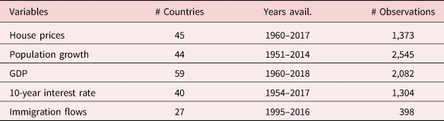
Our analysis certainly omits many variables that can potentially have explanatory power on house prices. Financial regulation, taxes, and changes in house price volatility or macroeconomic uncertainty over time can affect demand and supply conditions and thus house prices. Although a comprehensive analysis of house price dynamics is certainly worthwhile, we prefer to keep the analysis simple and focus on variables that first, are easy to measure and second, are considered standard in panel data regressions of population growth on house prices. Table 1 provides some descriptive statistics of our variables
Descriptive statistics

All variables are available at an annual frequency. Our analysis covers as many as 59 economies starting in many countries as early as 1950 and ending in 2018. A sample of countries included in our data include Australia, Austria, Belgium, Brazil, Canada, China, Czech Republic, Denmark, Estonia, Finland, France, Germany, Greece, Hungary, Iceland, India, Indonesia, Ireland, Israel, Italy, Japan, Korea, Latvia, Lithuania, Luxembourg, Mexico, the Netherlands, Norway, New Zealand, Poland, Portugal, Russia, Slovak Republic, Slovenia, South Africa, Spain, Sweden, Switzerland, the United Kingdom, the United States, and Turkey.
4.2 Regression
To estimate the effect of demographics on house prices, we use the following linear regression:

Y it is our main variable of interest namely house price growth of country i between the period t and t − 1. Moreover, X it represents the population growth of the country i in period t. Z it represents a vector of control variables, namely GDP, interest rates, and immigration inflows. Finally, D i is a country fixed effect and D t is a time fixed effect. Coefficient β gives us the change in house price growth if the population growth rate change by one percentage point. ε it is the residual in the regression.
4.3 Results
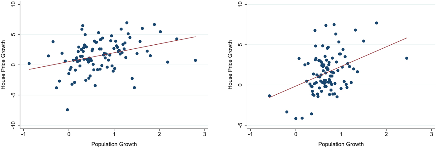
In this section, we report the results of our empirical exercise. Before reporting the result of the regression, we plot simple scatters of population growth and house price growth in Figure 1. The left panel of the figure plots the relationship without any fixed effects, while the right panel uses country fixed effects. Both scatters reveal a clear positive association between population growth and house price growth for our sample of OECD countries.
Scatter plot of house price growth and population growth for OECD countries.

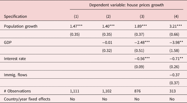
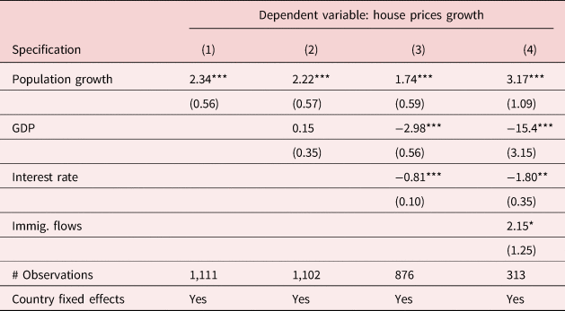
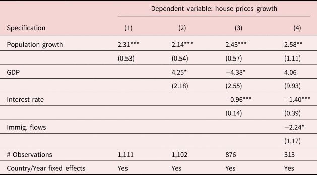
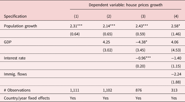
To analyze the effect controlling for other characteristics, we run the regression reported in equation (22). The total number of observations is more than a thousand since we have data on many countries for a relatively long period of time. We report our results using first, a specification without country or time fixed effects (Table 2), second, a specification with only country fixed effects (Table 3), and third, a specification with both country and time fixed effects (Table 4).
House prices and demographics (no country/year fixed effects)

Note: The standard errors are given in parentheses. One, two, and three stars denote significance at the 10%, 5%, and 1% levels, respectively.
House prices and demographics (w/ country fixed effects)

Note: The standard errors are given in parentheses. One, two, and three stars denote significance at the 10%, 5%, and 1% levels, respectively.
House prices and demographics (w/ country and year fixed effects)

Note: The standard errors are given in parentheses. One, two, and three stars denote significance at the 10%, 5%, and 1% levels, respectively.
4.3.1 The effect of population growth on house prices
Coefficient β gives the change (in percentage points) of house price growth if population growth increases by one percentage point. In all our specifications, we find a sizable and statistically significant positive effect of population growth on house price growth. In Table 2, which does not include any country or time fixed effects, the coefficient varies in the range of 1.47–3.21 percentage points. The inclusion of other controls does not substantially affect the coefficient. However, when we include immigration flows, the population growth coefficient increases dramatically which is perhaps explained by the sharp decrease in our available observations.
In Table 3, which controls for country fixed effects, the coefficient increases to the range of 1.74–3.17. So this implies that population growth has a stronger effect on house prices when we consider time variation within countries rather than looking across countries. In this case (country fixed effects), the coefficient decreases as we are adding more control variables with the exception of immigration flows which (as explained) substantially decreases the number of observations.
In Table 4, which controls for both country and time fixed effects, the coefficient is in the range of 2.14–2.58. This implies that when we control for both time and country fixed effects, the coefficient is less volatile across specifications with different controls.
Overall, we find a positive and statistically significant effect of population growth on house prices growth. What is worth nothing is that the effect is very robust to the inclusion of country fixed effects, time fixed effects, and other variables representing economic activity such as GDP, interest rate, and immigrations flows. This is exactly what our theoretical model predicts. A higher fraction of young people in the economy increases the demand for houses and increases house prices.
4.3.2 The effect of other economic and demographic characteristics on house prices
We discuss here the effect of our control variables on house prices. There is no clear effect of GDP on house prices from our regressions. Most specifications indicate a negative relationship, while others suggest a positive relationship (e.g., Table 4, columns 2 and 4). Moreover, very often the relationship is not statistically significant and it seems to be affected by the inclusion of interest rates.
The relationship between house prices and interest rate is more robust. Higher interest rate is associated with a smaller growth in house prices. Intuitively, when the cost to purchase a house is low, the demand is high which accelerates house price growth. Finally, we get a negative coefficient between house price growth and immigration flows. Nonetheless, these estimates are based on a small number of observations and the coefficients are not statistically significant.
4.4 Diagnostic checks
In this section, we perform some standard diagnostic tests regarding panel data analysis. We first explore our estimates if we cluster standard errors by country. We next evaluate if a fixed effect or a random effect specification is more appropriate for our exercise by running a Hausman test.
4.4.1 Clustering standard errors by country
It is possible that our standard errors are contaminated by correlation between the observations. To check this, we use the same regression as in section 4.3, but now we cluster standard errors at the country level. Our assumption implies that observations are correlated within a country but independent across countries (clusters). Table 5 replicates the specification in Table 4 (with country and time fixed effects) but cluster standard errors at the country level. So naturally, the coefficients are identical but the standard deviation changes. As we can see from Table 5, when we cluster standard errors at the country level, the standard errors increase slightly but coefficients are statistically significant at 1%. Once more, the only exception is the specification which controls for immigration flows which feature a small number of observations.
House prices and demographics (cluster S.E. by country)

Note: The standard errors are given in parentheses. One, two, and three stars denote significance at the 10%, 5%, and 1% levels, respectively.
4.4.2 Fixed effects vs. random effects: Hausman test
To evaluate if a fixed effect or a random effect model is more appropriate for our exercise, we run a Hausman test (Table 6). The test evaluates whether errors are correlated with the regressors or not. The null hypothesis in the test is that they are correlated.
Hausman test

Note: The table reports the Hausman test for analyzing the difference between fixed effect and random effect coefficient. One, two, and three stars denote significance at the 10%, 5%, and 1% levels, respectively.
Since the probability is higher than 5%, which implies that the difference is not significant, we conclude that the fixed effect model does not produce significantly different results from the random effect model.
5. Conclusion
In this paper, we analyze the relationship between house prices and demographics. The goal of the paper is to explain how aging population affects house prices. The question was approached in two steps. First, we built an overlapping generation model with a tradable asset which we think as a house. In every period, the house is being sold by old people to young people. If there is smaller population growth, then there would be an oversupply of houses in the market leading to a decrease in house prices. We establish this mechanism explicitly by showing how the equilibrium asset price is determined and how it is affected by demographics.
In the second step of the exercise, we provide empirical evidence of the proposed theoretical link. In particular, we collect data on house prices and demographics from the OECD. We find that countries that experience a faster population growth relatively to other countries also experience a higher house price growth relative to these countries. We find our empirical results to be robust to the inclusion of country and time fixed effects. Although this paper focuses on house prices, the basic mechanism applies for a variety of assets such as stocks, bonds, and precious metals. In future research, we intend to explore empirically the relationship between demographics and interest rates of financial assets such as government bonds or house mortgages.
Acknowledgements
I thank the Editor and an anonymous referee for extremely useful comments. For extremely useful suggestions and invaluable guidance throughout this project, I thank Karel Bruna. For helpful discussions and advice, I also thank Marios Karabarbounis and Nika Lazaryan. This paper was written with the assistance of F1/18/2017 project IGA in the University of Economics, Prague entitled “Macro-Financial Stability and Financial Cycle in Countries with Negative Net Investment Position.”