1. Introduction
In 1904, Lord Rayleigh (1842–1919) and his collaborator Sir William Ramsay (1852–1916) were awarded the Nobel Prize in physics and chemistry, respectively, primarily for their role in the discovery of argon, an inert gas in the atmosphere. The averse reaction to this discovery by Mendeleev (1834–1907) might have been the main reason for his not being awarded the Nobel prize in chemistry in 1906 (see Gordin Reference Gordin2004).
The discovery of argon resulted from a careful unraveling of an empirical discrepancy, initially detected by Rayleigh when measuring the density of nitrogen gas produced by two different procedures. After a long trial-and-error process based on a carefully designed sequence of experiments and guided by an informal (by today's standards) analysis of the resulting data (Larsen Reference Larsen1990), Rayleigh and Ramsay reached the conclusion that the atmospheric air contains argon, a hitherto unknown element.
The primary objective of this article is to revisit this historical episode, with a view to bringing out and systematizing this piecemeal learning from error that led to the discovery of argon. The error-statistical perspective (Mayo Reference Mayo1996) is used to systematize and formalize these scientists’ resourceful ways and strategies for detecting, eliminating, and obviating error as well as dealing with Duhemian problems and underdetermination issues (see Chalmers Reference Chalmers1999) as they arose in the context of their local research settings.
2. Why Is This Historical Episode Interesting?
The historical episode that led to the discovery of argon is interesting from the philosophy of science perspective for several reasons. First, it constitutes a case in which new scientific knowledge was not the result of a successful prediction from a well-established high-level theory but began as an empirical discrepancy detected at a ‘local’ (experimental) level while carrying out ‘normal’ science. This discrepancy triggered a sequence of investigations that led to the accumulation of local experimental knowledge (Mayo Reference Mayo1996), which eventually gave rise to a major revision of the periodic table and contributed to a new understanding of the nature of ‘matter’ more generally.
Second, the discovery of argon provides an example wherein the careful analysis of the data from a sequence of experiments guided scientists to pursue systematic ways in addressing the ensuing Duhemian problems and underdetermination issues and eventually led to unequivocal evidence for the existence of argon. This episode could potentially shed light on a number of philosophical issues, including the nature and justification of learning from data, the theory-data confrontation, and the nature of triggering mechanisms for large-scale theory change (see Mayo Reference Mayo, Mayo and Spanos2010).
Third, the statistical analysis performed by these scientists in the 1890s is particularly interesting because it is technically primitive by today's standards but highly sophisticated from the inductive-reasoning perspective. Indeed, this episode can be used to exemplify the potential role of experimental methods in conjunction with data analysis in addressing key philosophical problems as they arise in practice (see also Giunta Reference Giunta1998). These include how to determine the presence of a genuine anomaly, how to identify its cause, and whether its explanation calls for entirely new concepts and theories and even how to proceed in search of such more adequate explanations.
Last, the attempt to formalize the ‘learning-from-error’ process can help to demarcate the potential of the error-statistical perspective to account for and formalize different procedures and strategies used by scientists at the trenches in their attempt to circumvent Duhemian ambiguities (Staley Reference Staley2004). The most crucial Duhemian ambiguity pertaining to data-based inferences is whether the primary hypothesis is false or the auxiliary inductive premises invoked in testing it are invalid.
It is important to distinguish at the outset between error-statistical reasoning, which underlies learning from data in the presence of limited data, uncertainty, impurities, and noise (Mayo Reference Mayo1996), and the formal frequentist inference procedures developed in the 1930s by Fisher, Neyman, and Pearson (see Cox and Hinkley Reference Cox and Hinkley1974). The former offers a broader framework aiming to provide a more naturalistic perspective on philosophical problems of evidence and inference. Frequentist statistics provides a narrower special case grounded on probabilistic concepts aiming to systematize and formalize discerning scientific intuition in analyzing data, with a view to drawing reliable inferences. This should be contrasted with a Bayesian reconstruction (see Howson and Urbach Reference Howson and Urbach2005) in which one selects the prior probabilities to provide support for a certain narrative of the historical episode viewed retrospectively.
Section 3 summarizes the story of the discovery of argon, paying particular attention to the dialectic between perceptively mapped-out hypotheses and the inferences based on data resulting from carefully designed experiments that guide the search. Section 4 aims to make a case that Rayleigh's discerning intuition, implicit in his analysis of the experimental data, can be adequately accounted for and formalized by the error-statistical approach. Particular attention is paid to his endeavors to secure the reliability of his substantive inferences.
3. The Story of the Discovery of Argon
The story of the discovery of argon is well documented in chemistry (Wolfenden Reference Wolfenden1969; Giunta Reference Giunta2001, inter alia). The idea here is to provide a brief summary of that history, with a view to bringing out the ‘learning-from-data’ perspective of the dialectic between scientific hypotheses and the evidence from data resulting from a sequence of carefully designed experiments. This provides a prelude to the formalization of this learning process in the context of the error-statistical framework in section 4.
Rayleigh's investigations that led to the discovery of argon began in the early 1890s with an attempt to measure the atomic weight of nitrogen after his successes in determining the atomic weights of oxygen and hydrogen by evaluating their density. The story began routinely as another day at the lab, where he produced nitrogen gas from atmospheric air by removing the other known constituents. The conventional wisdom at the time was that atmospheric air was “a mixture of oxygen, nitrogen, and small quantities of carbon dioxide and water vapour, together with a trace of ammonia” (Ramsay Reference Ramsay1915, 148). The original procedure he used was to ‘bubble air through liquid ammonia’ and then pass it through a hot tube.
3.1. The Initial Detection of an Empirical Discrepancy
Rayleigh was ready to publish his results but decided to cross-check them using additional experiments in order to eliminate any potential errors that might be due to the particular method of production. The idea behind this move is that when several independent methods of producing nitrogen give rise to the same result within well-defined margins of experimental error, the evidence for the measured density is strengthened. This is an example of securing the robustness of a result using the argument from coincidence (Hacking Reference Hacking1983). To his surprise, when he weighed the nitrogen produced by the more traditional method of ‘treating air with hot copper’, “[it] proved to be one-thousandth part heavier than that obtained by the ammonia method; and on repetition, that difference was only brought out more clearly” (Rayleigh Reference Rayleigh1895, 702). After some additional investigation, he concluded that this discrepancy was (i) reproducible and (ii) could not be explained away as due to experimental error, whose magnitude was established by Rayleigh's earlier extensive work in measuring the density of oxygen and hydrogen.
3.2. Is the Observed Discrepancy Real or an Artifact?
Instead of trying to explain away the observed discrepancy, Rayleigh devised various experiments to bring it out more clearly. In particular, after realizing that—in addition to the nitrogen already in the atmospheric air—part of the nitrogen produced by his original method of treating air with liquid ammonia might be due to the reaction of ammonia with the oxygen in the air, he replaced air with pure oxygen to produce nitrogen of an entirely ‘chemical’ origin. Comparing this chemical nitrogen with the ‘atmospheric’ nitrogen produced by treating air with hot copper resulted in magnifying the discrepancy fivefold (Rayleigh Reference Rayleigh1895). This provided the initial clear clue that atmospheric nitrogen might contain unknown impurities.
To investigate that initial clue more thoroughly and appraise its robustness, Rayleigh proceeded to devise and apply a variety of different methods to produce atmospheric and chemical nitrogen. His objective was twofold. First, to ensure that both broad methods of producing nitrogen—using four different techniques for each—were giving rise to a homogeneous product. He understood that without this as a precondition, it would have been impossible to secure evidence for his second objective: to establish that the detected discrepancy was robust to the particular process, instruments, or chemicals used and was solely due to the difference between atmospheric and chemical nitrogen. The idea is that establishing the robustness of the discrepancy provides strong evidence of a real effect (Mayo Reference Mayo1996, 66).
The statistical analysis performed on these data by Rayleigh was technically rudimentary (by today's standards) but highly sophisticated in terms of his use of inductive reasoning. His primary tool was the method of ‘averaging’, going back to Gauss in 1809, which was known at that time as a way to enhance the reliability of estimating the magnitude of a ‘true’ quantity when the observed data differ from it by nonsystematic (white-noise) errors (see Stigler Reference Stigler1986). More formally, the sample mean

provides a more precise estimate of the true mean (E Zk = μ) than any one individual observation. This is because the mean of  $\overline{Z}$ is equal to μ, and its variance is n times smaller than that of any one component Z k—say
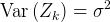 $\mathrm{Var}\,(Z_{k}) =\sigma ^{2}$ for
 $k=1,\, 2,\,\ldots \, ,\, n$—in the sense that

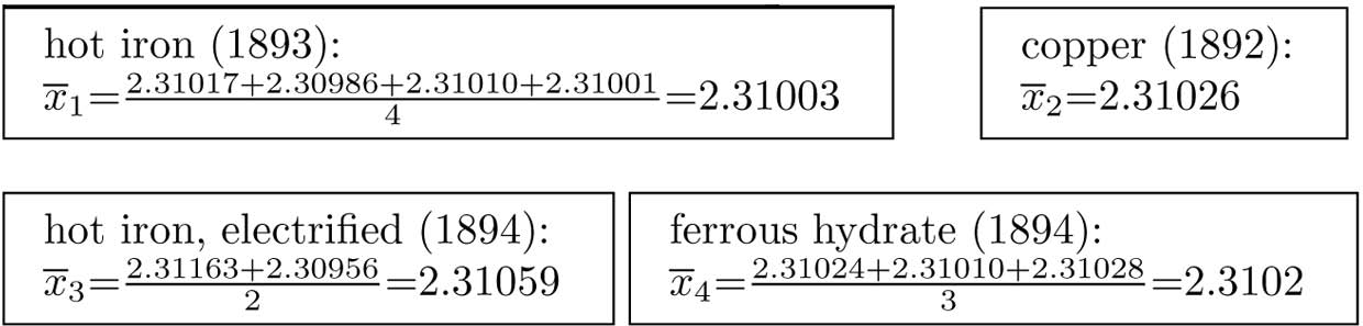
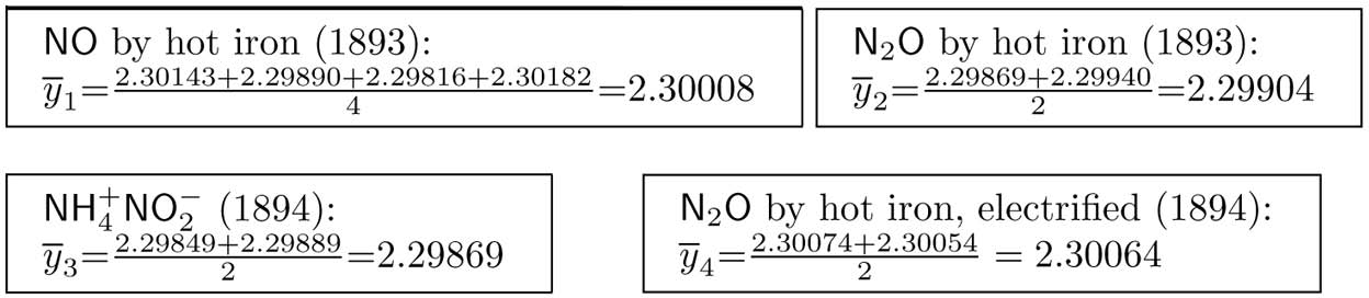
Rayleigh used the averaging in equation (1) for three different but interrelated purposes. First, he used it to enhance the ‘precision’ of the estimates associated with each different method of producing nitrogen, as shown in figures 1 ( $\overline{x}_{1},\,\ldots \, ,\,\overline{x}_{4}$) and 2 (
 $\overline{y}_{1},\,\ldots \, ,\,\overline{y}_{4}$). Second, he used averaging to ‘smooth out’ nonsystematic errors in assessing the homogeneity (nonsignificant differences) within each group (atmospheric or chemical) by comparing the individual observation with the group average. For atmospheric nitrogen, Rayleigh used four (fig. 1) different techniques to eliminate the oxygen: hot iron, ferrous hydrate, hot iron electrified, and copper. Each of the four methods is used to obtain an average, expecting that there will be some (small) variability even if they are all measuring the same unknown value. The question is whether the values are ‘close enough’ (within the experimental error bounds) to be regarded as homogeneous.
Atmospheric nitrogen.

Chemical nitrogen.

The smallness of the differences between each  $\overline{x}_{1},\,\ldots \, ,\,\overline{x}_{4}$,

and the group average  $\overline{x}=2.310221$ led him to infer that all four production techniques were giving rise to the same (homogeneous) product (see Rayleigh Reference Rayleigh1894, 343). That is, the deviations within the group were considered nonsystematic and inside the margins of the established experimental error (Rayleigh Reference Rayleigh1893).
Similarly, he used four different techniques to produce chemical nitrogen: nitric oxide (NO) by hot iron, nitrous oxide (N2O) by hot iron, N2O by hot iron electrified, and ammonium nitrite ( $\mathrm{NH}\,^{+}_{4}$
 $\mathrm{NO}\,^{-}_{2}$). Again, the smallness of the differences between each
 $\overline{y}_{1},\,\ldots \, ,\,\overline{y}_{4}\,\,$,

and the group average  $\overline{y}_{1}=2.299706$ indicated that all four chemical techniques were giving rise to a homogeneous product.
The third application of averaging by Rayleigh was to use the difference between the two overall group averages,

to argue that it was significantly different from zero because the magnitude of equation (5) was many times bigger than the average differences within the atmospheric nitrogen in figure 1 and the chemical nitrogen in figure 2. On the basis of equation (5), Rayleigh concluded, “The difference is about 11 milligrams, or about one-half per cent; and it was sufficient to prove conclusively that the two kinds of nitrogen—the chemically derived nitrogen and the atmospheric nitrogen—differed in weight, therefore, of course, in quality, for some reason hitherto unknown” (Reference Rayleigh1895, 702).
The difference of 11 milligrams was deemed—because of his extensive experience—well outside the experimental error range for this type of experiment (Rayleigh Reference Rayleigh1895). Ramsay, reflecting on the accuracy of Rayleigh's early results, asserted, “It is evident from inspection of the numbers quoted above that the accuracy of the density determination may be trusted to within 1 part in 10,000” (Reference Ramsay1915, 155).
3.3. How Reliable Was Rayleigh's Primary Inference?
The term “reliability” is used to denote probing for errors and ascertaining the relevant error probabilities at three different levels.
3.3.1. Experimental Reliability
Rayleigh was well aware of the ruining effects of systematic errors on the results of his experiments, and he discusses extensively the importance of securing “the unsystematic character” of experimental errors and made concrete suggestions on how to achieve that in measuring the density of gases (Rayleigh Reference Rayleigh1893, 135; see also Larsen Reference Larsen1990). In his experiments, he used every conceivable precaution to guard against impurities and uncontrolled influences: “I need not spend time in explaining the various precautions that were necessary in order to establish surely that conclusion. One had to be on one's guard against impurities, especially against the presence of hydrogen, which might seriously lighten any gas in which it was contained” (Rayleigh Reference Rayleigh1895, 702).
3.3.2. Statistical Reliability
At the level of the statistical analysis of data, Rayleigh's reasoning was based primarily on a comparison of the difference between the overall group averages  $( \overline{x}-\:\overline{y}) $ against the discrepancies within each group average (
 $[ \overline{x}_{1}-\:\overline{x}] ,\,\ldots \, ,\,[ \overline{x}_{4}-\:\overline{x}] $,
 $[ \overline{y}_{1}-\overline{y}] ,\,\ldots \, ,\,[ \,\overline{y}_{4}-\:\overline{y}] $). Viewed retrospectively, this can be best understood as an informal version of the t-test based on
 $( \overline{x}-\:\overline{y}) / [ \mathrm{Var}\,( \overline{x}-\:\overline{y}) ] ^{1/ 2}$. It turns out that this test constitutes a most effective procedure for detecting any departure from zero when present (see sec. 4).
In addition, Rayleigh was careful to assess the crucial assumption of homogeneity underlying the validity of his primary conclusion that the discrepancy between the density of atmospheric and chemical nitrogen was real and not an artifact. What is remarkable about his move, viewed retrospectively, is that it constitutes a crude, but effective, misspecification test for assessing the validity of his premises of inference (see sec. 4 for further discussion).
3.3.3. Substantive Reliability
Rayleigh used a blend of theoretical and experimental knowledge, in conjunction with data analysis, to go beyond the empirical discrepancy and establish a substantive discrepancy, which was instrumental in leading to the discovery of argon. His primary tools were ‘learning from trial and error’ and ‘reasoning from coincidence’ (see Chalmers Reference Chalmers1999) to secure the reliability and robustness of his conclusions concerning the magnitude and nature of the substantive discrepancy.
3.4. ‘Reasoning from Error’ to Establish the Discrepancy
Rayleigh published his preliminary results on the density of nitrogen in 1893, cautioning the reader about the existence of an empirical discrepancy. He was so concerned that he sought advice from other scientists, especially chemists, by publishing a letter in Nature in 1892, inviting them to suggest possible explanations of the discrepancy, but none of the early tendered explanations were helpful (Rayleigh Reference Rayleigh1895, 702). On the basis of his own evidence, Rayleigh reached a tentative conclusion: “Upon the assumption that similar gas should be obtained by both methods, we may explain the discrepancy by supposing either that [h1] the atmospheric nitrogen was too heavy on account of imperfect removal of oxygen, or that [h2] the ammonia nitrogen was too light on account of contamination with gases lighter than pure nitrogen” (Reference Rayleigh1894, 340).
The established theoretical knowledge at the time, used in conjunction with his data, played a crucial role in rendering the hypothesis h1 virtually impossible. Rayleigh argued that since the density of oxygen and nitrogen is similar, h1 must be false because the observed discrepancy would have required the produced nitrogen gas to contain a huge quantity of oxygen—“the nitrogen should have contained 1/30 of its volume of oxygen, or 1/6 of that present in air” (Reference Rayleigh1894, 341)—which was impossible on theoretical grounds. His experiments also rendered h2 rather implausible: “Of the possible impurities lighter than nitrogen, those most demanding consideration are hydrogen, ammonia, and water vapour. The last may be dismissed at once, and the absence of ammonia is almost equally certain. The question of hydrogen appears the most important. But this gas, and hydrocarbons, such as CH4, could they be present, should be burnt by the copper oxide; and the experiments already referred to, in which hydrogen was purposefully introduced into atmospheric nitrogen, seem to prove conclusively that the burning would really take place” (342).
Hence, the potential culprits (oxygen in h1 and hydrogen in h2) were eliminated by a combination of theoretical knowledge and a rudimentary analysis of the data from his experiments. His arguments constitute exemplars in dealing with Duhemian ambiguities by using existing knowledge in conjunction with reliable data to obviate potential errors, as well as posing sharp questions at the experimental level that could potentially yield incisive answers.
Rayleigh went on to consider and eliminate other possible explanations that might have given rise to h2, including the possibility that chemical nitrogen might have been contaminated by dissociated (i.e., monatomic) nitrogen, N1. In addition, he stored the chemical nitrogen for 8 months and reweighed it in order to ensure that the discrepancy persisted.
Reflecting on the hypotheses h1 and h2, one can see that they did not amount to a partition of the set of all possible explanations. In a move to render them exhaustive, Rayleigh went on to effectively recast the original hypotheses as follows:
 $\mathbf{h}^{\prime }_{1}$. The atmospheric nitrogen was too heavy because it contained a heavier gas.
 $\mathbf{h}^{\prime }_{2}$. The chemical nitrogen was too light because it contained a lighter gas.
At the end of a trial-and-error process, Rayleigh's primary conclusion was that “altogether, the balance of evidence seemed to incline against the hypothesis of abnormal lightness in the chemically derived nitrogen being due to dissociation, and to suggest strongly, as almost the only possible alternative, that there must be in atmospheric nitrogen some constituent heavier than true nitrogen” (Reference Rayleigh1895, 703). That is, Rayleigh's evidence pointed strongly toward  $\mathrm{h}\,^{\prime }_{1}$.
His 1892 letter in Nature seeking advice from other scientists eventually prompted the chemist William Ramsay in April 1894 to initiate a collaborative research effort that began by probing hypothesis  $\mathrm{h}\,^{\prime }_{1}$ from a number of different perspectives. The nature of their collaboration can be described as ‘working in parallel’ with “letters passed almost daily between them, describing the results of experiments which one or other had made” (Ramsay Reference Ramsay1915, 166). See Wolfenden (Reference Wolfenden1969) for further details on the nature of the collaboration and references to controversies concerned with Ramsay's role in the discovery of argon.
3.5. Explaining the Discrepancy by Identifying a Heavier Gas
A particularly promising suggestion they decided to pursue in earnest was to revisit an older experiment in 1783 by Cavendish, who demonstrated that after both the oxygen and the nitrogen were extracted from atmospheric air, there was a small residue that “amounted to about 1/120 part of the nitrogen taken” (Rayleigh Reference Rayleigh1895, 704). Cavendish's result was duly confirmed by Rayleigh using a larger-scale experiment with better apparatuses. In light of that, Ramsay proceeded to devise an experiment to remove all nitrogen from the sample of atmospheric nitrogen by passing it repeatedly over heated magnesium, with which nitrogen reacts to form magnesium nitride—a solid. This experiment left a 1% residual that was denser than nitrogen and would not react with any other chemical element.
To shed further light on the source of the residue from atmospheric air, Rayleigh devised a diffusion experiment in which atmospheric nitrogen was passed through a long sequence of porous clay pipes surrounded by a vacuum. The portion of nitrogen diffused through the clay was less dense than the remainder, indicating that the heavier gas must have been in the original atmospheric air. This sequence of experiments provided strong evidence against  $\mathrm{h}\,^{\prime }_{2}$: “the conclusion seems inevitable that ‘atmospheric nitrogen’ is a mixture and not a simple body” (Rayleigh and Ramsay Reference Rayleigh and Ramsay1895, 208).
To check the robustness and strengthen the reliability of this conclusion, the nitrogen from chemical nitrogen was removed by passing it repeatedly over heated magnesium, and no significant residue was detected. “While these experiments were in progress, Lord Rayleigh was occupied in preparing nitrogen from other sources, and in determining its density; and in every case it was evident that nitrogen from all sources except the atmosphere weighed somewhat less than atmospheric nitrogen” (Ramsay Reference Ramsay1915, 165).
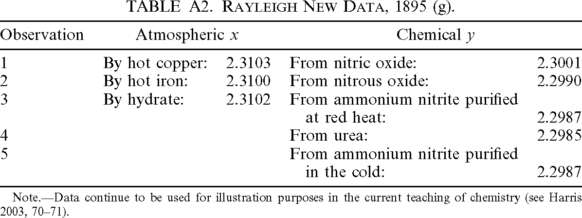
Rayleigh's new (more precise) data (table A2) enhanced the discrepancy:

affirming his initial findings beyond any reasonable doubt. Having established the presence of the heavier gas in atmospheric nitrogen, Rayleigh and Ramsay went a step further and argued that “if the newly discovered gas were not in the atmosphere, the discrepancies in the density of ‘chemical’ and ‘atmospheric’ nitrogen would remain unexplained” (Reference Rayleigh and Ramsay1895, 235). In Mayo's terminology, their claim amounts to hypothesis  $\mathrm{h}\,^{\prime }_{1}$ passing a severe test, in the sense that it “has withstood a scrutiny that it would very likely have failed, were it not correct” (Reference Mayo1996, 30).
3.6. Was the Heavier Gas a New Monatomic Element?
The last potential explanation they proceeded to eliminate was
h3. The heavier gas was triadic nitrogen N3.
The primary evidence in favor of a new element was provided by the spectral analysis applied by Ramsay to the residue from the improved Cavendish experiment that indicated hitherto unidentified spectral lines. The crucial evidence that the new element was monatomic came from the measurement of the specific heat capacities of the residual gas at constant pressure ( $C_{p}$) and at constant volume (
 $C_{v}$). It turned out that the Clausius relationship
 $K/ H=( 3/ 2) ( [ C_{p}-C_{v}] / C_{v}) $ (Scerri Reference Scerri2007), from kinetic theory, where K denotes the translational energy and H the total kinetic energy, just about eliminated the possibility of a nonmonatomic structure for the residual gas. The evaluation of the ratio's empirical value at (C p/C v) ≃ 1.65 implied that
 $K\simeq H$, which indicated strongly that “the gas has no energy except energy of translation of its molecules” (Rayleigh Reference Rayleigh1895, 710).
Weaving together all these pieces of corroborating evidence using systematic reasoning from error, Rayleigh and Ramsay were able to make a very strong case that the detected discrepancy is due to a hitherto unknown monatomic element found in the atmosphere. They called it argon (the Greek word for ‘inactive’) because of its chemical inertness. That is, their inference was that a more specific hypothesis passed a severe test in the sense of Mayo (Reference Mayo1996):
 $\mathbf{h}^{\prime \prime }_{1}$. Atmospheric nitrogen was more dense because it contained a heavier gas from atmospheric air, identified as a new monatomic element (argon).
Rayleigh and Ramsay made a preliminary (oral) announcement of their discovery of a ‘new constituent gas’ in atmospheric air at the Oxford meeting of the British Association in August 1894 (see Ramsay Reference Ramsay1915, 166). They submitted their discovery of argon for the 1894 Smithsonian Institutions’ Hodgkins prize, which they duly won; no publication before submission was a precondition. They presented their results to the Royal Society in early 1895 (see Rayleigh and Ramsay Reference Rayleigh and Ramsay1895).
3.7. Averse Reaction from the Old Guard
Predictably, the original 1894 claim for the discovery of argon was met with skepticism bordering on hostility. Several famous chemists of that period, including James Dewar and Dmitri Mendeleev, refused to accept the evidence for  $\mathrm{h}\,^{\prime \prime }_{1}$, and instead argued fervently in favor of h3 because it accorded well with the prevailing theoretical framework. In contrast,
 $\mathrm{h}\,^{\prime \prime }_{1}$ raised thorny problems because argon (i) did not fit into Mendeleev's periodic table—attempts to fit it, created a “pair reversal” problem with potassium—and (ii) its inertness raised the possibility of a zero-valence group of elements and made it impossible to study its properties (e.g., atomic weight) using chemical processes. For a detailed discussion on these issues, see Wolfenden (Reference Wolfenden1969) and Giunta (Reference Giunta2001).
Rayleigh was so frustrated by the incessant and unjustified (in his mind) criticisms by various chemists that he would herald his return to physics by declaring that in that field “second rate men seem to know their place” (Brock Reference Brock1992, 336). The hostility from Mendeleev and his group against  $\mathrm{h}\,^{\prime \prime }_{1}$ did not dissipate until the other noble gases were discovered in 1895 by Ramsay (helium), 1898 by Ramsay and Travers (neon, krypton, xenon), and 1900 by Dorn (radon); see Scerri (Reference Scerri2007).
3.8. Experimental Knowledge and Its Role in Theory Change
In summary, argon's discovery began as a mere empirical discrepancy, detected ‘locally’ in a particular experiment, but the subsequent search for adequate explanations within the prevailing theoretical framework led to a sequence of interconnected experiments that were catalytic in undermining that framework. The discovery of argon and the other noble gases initially added to the experimental knowledge, in the form of warranted claims established by data-driven procedures. This new experimental knowledge could not be accommodated within the then-prevailing theoretical framework, giving rise to a crisis that eventually led to a change of paradigms (Kuhn Reference Kuhn1970).
A new theoretical framework, which could accommodate this experimental knowledge, began to be fleshed out with Moseley's 1914 proposal to replace atomic weights with atomic numbers (the total number of protons in the element's atomic nucleus). Using atomic numbers resolved the existing inconsistencies with Mendeleev's periodic table, accommodating meticulously the noble gases (Scerri Reference Scerri2007).
4. Error Statistics and Formal Inductive Inference
Going from the initial discrepancy between atmospheric and chemical nitrogen to inferring that it was due to the presence of argon in atmospheric air, Rayleigh and Ramsay had to deal with numerous Duhemian ambiguities and underdetermination problems. First, they had to establish that the discrepancy was real (not an artifact) and evaluate its magnitude. Second, they had to trace the discrepancy, initially to atmospheric nitrogen and then to the presence of a new constituent gas (heavier than nitrogen) in atmospheric air. Third, they had to narrow that down, initially to a new element and then to a monatomic gas.
Looking at the sequence of experiments performed by Rayleigh and Ramsay from the error-statistical perspective, one can make a case that what did most of the work in guiding these two pioneers to the discovery of argon was their intuitively sound inductive reasoning in drawing inferences on the basis of the data at a local (experimental) level. This reasoning is particularly useful in this case because, when formalized, it enables one to combine experimental data and statistical concepts and methods in uncovering and explaining what really gave rise to the experimental knowledge. This is achieved by a pertinent embedding of a material experiment, and the data  $\mathbf{z}_{0}$ it gives rise to, into an appropriate statistical model. The key to pertinence is provided by the adequacy of the embedding statistical model in the sense that it accounts for the regularities in data
 $\mathbf{z}_{0}$. As argued in section 4.6, this can help in dealing with Duhem's and underdetermination problems and secure the reliability of inferences, enabling one to separate real effects from artifacts.
A question that arises is whether such an interpretation is even warranted in view of the fact that the inference methods used were not formally developed until the 1930s. By the same token, modern formal logic was developed in the early twentieth century, but nobody is likely to argue that sound deductive reasoning was not practiced before then. It is argued that the informal statistical reasoning used by these scientists is highly sophisticated from the inductive (learning-from-data) perspective, despite the absence of the formal modern statistical methods. Indeed, the latter can be used retrospectively to formalize their informal inductive reasoning.
The framework used to formalize and interpret the informal statistical analysis that led to the discovery of argon is known as error statistics. The term was coined by Mayo (Reference Mayo1996) to denote a refinement/extension of the framework for frequentist inference associated with Fisher, Neyman, and Pearson (see Spanos Reference Spanos2007).
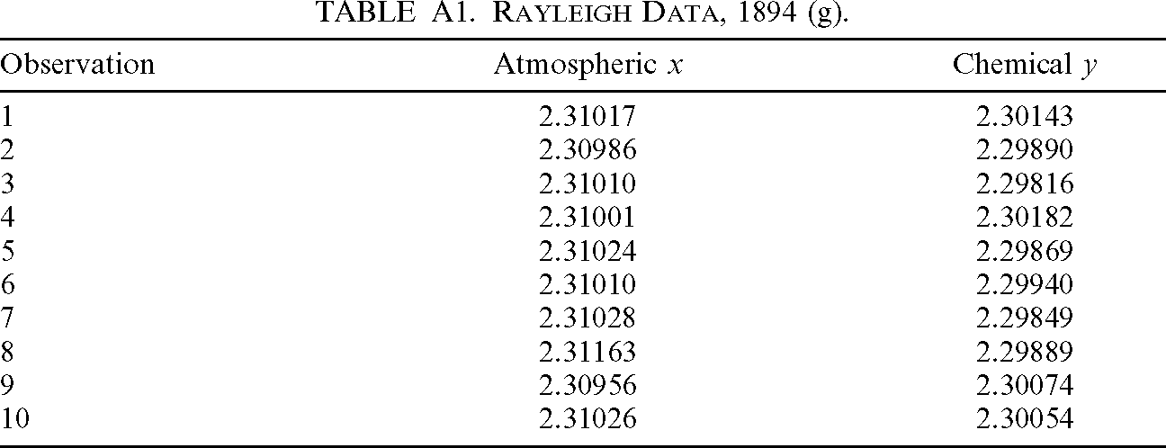
As argued in section 3, Rayleigh's intuitive learning-from-data reasoning was remarkably sophisticated in certain respects. The following discussion aims to make this case by answering these questions: How can one formalize and systematize (i) the procedures used by Rayleigh to reach the conclusion—using his data (table A1)—that the empirical discrepancy he detected is real, and (ii) how can one assess the reliability of his particular inferences?
4.1. Embedding a Material Experiment into a Statistical Model
From the error-statistical vantage point, it is known that the reliability of any data-based inference depends on the validity of certain probabilistic assumptions, collectively known as a statistical model that specifies the inductive premises of inference. We can bring out these implicit probabilistic assumptions by retrospectively unveiling the statistical model into which Rayleigh's material experiment, yielding data  $\mathbf{z}_{0}=( x_{1},\, x_{2},\,\ldots \, ,$
 $x_{n_{1}},\, y_{1},\, y_{2},\,\ldots \, ,\, y_{n_{2}}) $, can be appropriately embedded. The implicit presupposition is that
 $\mathbf{z}_{0}$ constitute a realization of a sample
 $\mathbf{Z}$ of the form

whose probabilistic structure is specified by

where NIID (μ, σ 2) denotes normal, independent, and identically distributed, with mean μ and variance σ 2. Model  $\mathstrut{\cal M} _{0}$ is known as the simple normal model. That is, the data
 $\mathbf{z}_{0}$ in table A1 are viewed as a typical realization of the sample
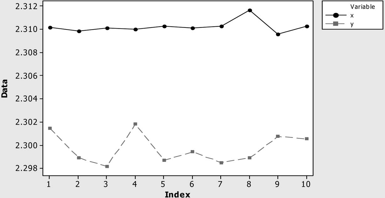
 $\mathbf{Z}$ whose probabilistic structure is given in equation (7). The k-plots of this data in figure A1 suggest that the IID assumptions are not unreasonable (see Spanos Reference Spanos1999, chap. 5).
Are the IID Assumptions Valid for  $\mathbf{z}_{0}$?

Although unaware that he was invoking such formally defined probabilistic assumptions, Rayleigh in effect did his level best to ensure their validity indirectly via his design of experiments by (i) ensuring that his experimental setups adequately secured the physical independence of the different production processes and (ii) securing the homogeneity of the produced nitrogen within the two (chemical and atmospheric) processes. He knew intuitively that to secure the reliability of his inference he needed i and ii. Does Rayleigh's averaging (implicitly) invoke the IID assumptions? The short answer is yes because without these assumptions the result in equation (2) is no longer valid. Instead,

and thus the enhanced precision and smoothing benefits of averaging are vitiated.
What about the Normality Assumption?
Without a distributional assumption, one cannot derive accurate enough error probabilities on the basis of a sample size ( $n=10$) to establish the optimality and reliability of inference procedures relating to μ. This became apparent with Student's (1908) classic article but was systematized later on by Fisher (Reference Fisher1922) in an article that founded modern model-based inference based on finite sampling theory (any
 $n> 1$). Statistical inference before then relied almost exclusively on procedures based on a ‘large enough’ n.
4.2. Formalizing the Testing for the Presence of a Discrepancy
Viewed in the context of equation (7), Rayleigh's substantive question of interest can be framed in terms of the mean of atmospheric and chemical nitrogen, μ 1 and μ 2, respectively, to form the statistical hypotheses:

In this statistical context, it can be shown that an optimal (uniformly most powerful) test for equation (9) exists. The property of uniformly most powerful refers to the capacity of a test to detect any discrepancy  $\gamma \geq 0$ from the null
 $\mu =0$ with higher probability than any other
 $\alpha $-significance-level test. This optimal
 $\alpha $-level test
 $T_{\alpha }$ is defined in terms of a test statistic
 $\tau ( \mathbf{Z}) $ in conjunction with a rejection region
 $C_{1}( \alpha ) $:

where c α denotes the rejection value for a given α; for example, for  $\alpha =.05$,
 $c_{\alpha }=1.734$. That is,
 $H_{0}$ is rejected by any data
 $\mathbf{z}_{0}$ such that
 $\tau ( \mathbf{z}_{0}) > 1.734$; otherwise,
 $H_{0}$ is accepted.
Note that  $( \overline{X},\:\overline{Y},\: s^{2}_{1},\: s^{2}_{2}) $ denote estimators of the parameters
 $( \mu _{1},\:\mu _{2},$
 $\sigma ^{2}_{1},\:\sigma ^{2}_{2}) $, and
 $s^{2}_{12}$ is an estimator of
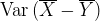 $\mathrm{Var}\,( \overline{X}-\overline{Y}) $. That is, the test statistic
 $\tau ( \mathbf{Z}) $ is a standardized (scaled by its standard deviation) distance between the two sample means, which is nothing more than a formalization of Rayleigh's informal comparison in equations (5) and (6).
The relevant type I error probability and power for this test are derived, respectively, from the following sampling distributions:

where “ $\stackrel{H_{0}}{\sim }\mathrm{St}\,( \nu ) $” reads “distributed under the null as Student's t with
 $\nu =( n_{1}+n_{2}-2) $ degrees of freedom,” and
 $\mathrm{St}\,( \delta ;\nu ) $ denotes a noncentral Student's t with
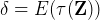 $\delta =E( \tau ( \mathbf{Z}) ) $ evaluated under H 1 (see Cox and Hinkley Reference Cox and Hinkley1974).
4.3. Establishing a Statistical Discrepancy
Let us apply formal statistical testing to appraise the informal analysis applied by Rayleigh. His data  $\mathbf{z}_{0}$ in table A1, based on
 $n_{1}=n_{2}=10$, yield the estimates

These, in turn, give rise to the observed test statistic:

with the associated p-value (.0000000), defined by

where  $\mathstrut{\Bbb P} ( .) $ denotes a probability function. The tiny p-value in conjunction with a small sample size, indicates that
 $\mathbf{z}_{0}$ provide strong evidence against the null (see Mayo and Spanos Reference Mayo and Spanos2006).
The result of the t-test in equation (11) indicates statistical significance, but that is not equivalent to Rayleigh's inference that atmospheric and chemical nitrogen have different weights. The latter refers to substantive significance, which does not follow automatically from statistical significance. Indeed, this is an example of the
Fallacy of Rejection. Evidence against H 0 is not evidence for a particular H 1.
This fallacy can arise when the test applied is oversensitive in the sense that it has enhanced capacity to detect even tiny discrepancies from H 0; this often arises when n is very large (Mayo Reference Mayo1996). There is an analogous fallacy in the case of a statistically nonsignificant result:
Fallacy of Acceptance. No evidence against H 0 is not evidence for it.
This can easily arise when the test applied is not sensitive enough to detect an existing discrepancy; this often arises when n is very small.
4.4. Establishing a Substantive Discrepancy
Historically, these two fallacies have bedeviled the traditional frequentist testing since the 1930s. To guard against these fallacies, one can adopt the more refined/extended error-statistical frequentist framework, wherein the accept/reject results and the p-values are scrutinized further using a postdata severity assessment (Mayo Reference Mayo1996). The idea underlying this assessment is to answer the basic question, when do data  $\mathbf{z}_{0}$ provide evidence for (or against) a hypothesis or a claim H? by establishing the discrepancy γ from H 0 warranted by test T α and data
 $\mathbf{z}_{0}$.
A test T α provides evidence for a hypothesis H only to the extent that the data  $\mathbf{z}_{0}$ accord with hypothesis H, and, in addition, such a good result would have been highly unlikely if H were false. When the null hypothesis in equation (9) is rejected, the relevant severity assessment concerns the largest discrepancy
 $\gamma \geq 0$ warranted by data
 $\mathbf{z}_{0}$. This results from evaluating ‘the probability of observing sample realizations
 $\mathbf{z}$ that accord less well with
 $\mu > \gamma $ than
 $\mathbf{z}_{0}$ do, under the scenario that
 $\mu > \gamma $ is false’, giving rise to the severity function (Mayo and Spanos Reference Mayo and Spanos2006):

For test  $T_{\alpha }\mathrel{\mathop:}= ( \tau ( \mathbf{Z}) ,\: C_{1}( \alpha ) ) $ in equation (10) and data
 $\mathbf{z}_{0}$ (table A1), the evaluation is based on

and yields the numerical results shown below.
| Relevant Claim |  $( \mu _{1}-\mu _{2}) > \gamma $ |
||||||
|---|---|---|---|---|---|---|---|
| γ | .008 | .009 | .01 | .0101 | .0105 | .011 | .012 |
 $\mathrm{SEV}\,( T_{\alpha }\mathrm{;}\,\:\mathbf{z}_{0}\mathrm{;}\,\:\mu > \gamma ) $ |
1.00 | .995 | .858 | .809 | .513 | .147 | .002 |
Assuming a high enough threshold for severity, say .85, the largest discrepancy between the means of the atmospheric (μ 1) and chemical (μ 2) nitrogen warranted by data  $\mathbf{z}_{0}$ on the basis of test T α is
 $( \mu _{1}-\mu _{2}) > .01$. This formally confirms closely Rayleigh's original substantive inference.
4.5. Statistical Adequacy and the Reliability of Inference
The reliability of all the above inferences depends crucially on the adequacy of the statistical model  $\mathstrut{\cal M} _{0}$ given in equation (7). Intuitively, a statistical model is considered adequate if ‘it accounts for the regularities in the data’. That is, when the particular statistical model is fitted to the data, what is left—the residuals—constitutes a white-noise (nonsystematic) process. A more formal way to state this is in terms of statistical adequacy: the probabilistic assumptions constituting
 $\mathstrut{\cal M} _{0}$ are valid vis-à-vis data
 $\mathbf{z}_{0}$.
The importance of statistical adequacy stems from the fact that it secures the reliability of inference by ensuring that the actual error probabilities approximate closely the nominal ones. The surest way to draw an invalid inference is to apply a .05 significance-level test when its actual—due to misspecification—type I error probability is closer to .99.
For example, the probabilistic assumptions constituting the simple normal model  $\mathstrut{\cal M} _{0}$ in equation (7) are
1. Normality:
$X_{k}\sim N( .) $, $Y_{k}\sim N( .) $, $k\in N\mathrel{\mathop:}= 1,\, 2,\,\ldots \} $.2. Constant means:
$E( X_{k}) =\mu _{1}$, $E( Y_{k}) =\mu _{2}$, for $k\in N$.3. Constant variance:
$\mathrm{Var}\,( X_{k}) =\mathrm{Var}\,( Y_{k}) =\sigma ^{2}$, for $k\in N$.4. Independence:
$\{ ( X_{k},\: Y_{k}) ,\: k\in N\} $ is an independent process.








How does one assess the validity of these assumptions? In practice, the assessment of these probabilistic assumptions takes the form of an informal check using graphical techniques, as well as a formal test using misspecification tests based on the residuals (see Mayo and Spanos Reference Mayo and Spanos2004).
4.5.1. Rayleigh's Appraisal of Assumption 2
Rayleigh concluded that the empirical discrepancy he detected was real, by comparing the between-group differences  $( \overline{z}-\:\overline{z}_{i}) $,
 $i=1,\: 2$, to assess whether they were ‘substantial enough’ relative to the within-group
 $(z_{ik}-\:\overline{z}_{i}) $,
 $k=1,\,\ldots \, ,\, n_{i}$, differences. He showed exceptional discerning intuition by recognizing that the homogeneity within each of the two broad groups of atmospheric and chemical nitrogen was a crucial precondition for the validity of his primary inference as formalized in equation (9).
From a modern perspective, one can formalize Rayleigh's assessment of the homogeneity within each group using an ANOVA test—initially proposed by Fisher and Mackenzie (Reference Fisher and Mackenzie1923). In the context of the statistical model  $\mathstrut{\cal M} _{0}$, this homogeneity represents assumption 2, and thus the ANOVA is a misspecification test, which, for two groups, with n 1 and n 2 observations (
 $n=n_{1}+n_{2}$), takes the form

where 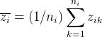 $\overline{z_{i}}=( 1/ n_{i}) \sum_{k=1}^{n_{i}}z_{ik}$,
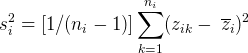 $s^{2}_{i}=[ 1/ ( n_{i}-1) ] \sum_{k=1}^{n_{i}}(z_{ik}-\:\overline{z}_{i}) ^{2}$,
 $i=1,\: 2$, denote the sample mean and variance for each group, respectively, and
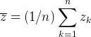 $\overline{z}=( 1/ n) \sum_{k=1}^{n}z_{k}$ is the overall sample mean,
 $F( 1,\: n-2) $ denotes the F distribution with
 $( 1,\: n-m) $ degrees of freedom, and
 $C_{1}( \alpha ) $ is the rejection region (see Cox and Hinkley Reference Cox and Hinkley1974). ANOVA results for atmospheric nitrogen are

( $p=.767$), and ANOVA results for chemical nitrogen are

( $p=.772$). On the basis of the observed value of both test statistics and the high p-values, one can conclude that there is no evidence against the homogeneity assumption. These results confirm (formally) Rayleigh's original informal inference.
4.5.2. Additional Misspecification Tests
How reliable were Rayleigh's inferences viewed from today's perspective? On the basis of the following misspecification tests, one can deduce that, in addition to assumption 2, assumptions 1 and 4 are valid, but 3 is invalid. Testing normality (assumption 1) using the Shapiro-Wilks test yielded  $\mathrm{S}\,- \mathrm{W}\,( \mathbf{z}_{0}) =.879$ (
 $p=.121$). Testing independence (assumption 4) using a runs test yielded
 $R( \mathbf{z}_{0}) =-0.000078$ (
 $p=.782$). Neither test indicates any departures from assumptions 1 and 4 (see Spanos Reference Spanos1999).
Testing variance equality (assumption 3) using  $v( \mathbf{z}_{0}) =( s^{2}_{2}/ s^{2}_{1}) =.000001724/ .000000292699=5.890$ (
 $p=.007$). The small p-value in conjunction with a small n provide evidence against 3. Remarkably, the larger variance from chemical nitrogen was actually noticed by Rayleigh: “the agreement of individual results is less close in the case of chemical nitrogen than of atmospheric nitrogen” (Reference Rayleigh1893, 344). A glance at figure A1 also confirms that. How does this departure affect the reliability of Rayleigh's inference? It does not. Despite the departure from assumption 3, the inferences concerning the primary hypothesis (eq. [9]) turn out to be robust. Alternative tests that take account of such a departure (Welch Reference Welch1938) give rise to almost identical error probabilities and, hence, inferences.
4.6. Dealing with Duhem's Problem and Underdetermination
The above discussion brings out the key role played by statistical adequacy in addressing Duhem's problem: it is impossible to test a scientific hypothesis in isolation because an empirical test of the hypothesis requires auxiliary assumptions (or hypotheses). This problem can be addressed via a pertinent embedding of the material experiment into a statistical model  $\mathstrut{\cal M} _{0}$ whose auxiliary assumptions can be assessed independently of the primary hypothesis of interest h—the difference in density between atmospheric and chemical nitrogen. The substantive hypothesis h is framed in the context of the statistical model
 $\mathstrut{\cal M} _{0}$ using the statistical parameters as in equation (9). The only auxiliary hypotheses one needs to invoke to secure the error reliability of inference are the model assumptions 1–4. In view of the fact that the validity of these assumptions pertains to the chance regularities in data
 $\mathbf{z}_{0}$ and can be assessed independently of h, the statistical adequacy of
 $\mathstrut{\cal M} _{0}$ ensures that no Duhemian ambiguities of the form, Is h false? or are any of the assumptions 1–4 invalid for data
 $\mathbf{z}_{0}$? arise in relation to the substantive inference.
In contrast, when the statistical adequacy of  $\mathstrut{\cal M} _{0}$ is unknown, relating statistical to substantive significance is highly problematic because the situation raises numerous Duhemian equivocations. For instance, it is not known whether the detected statistical significance is due to the presence of a substantive discrepancy or constitutes an artifact forged by a difference between nominal and actual error probabilities originating in departures from assumptions 1–4.
Statistical adequacy also sheds different light on the problem of underdetermination at the level of selecting statistical models. The problem with traditional discussions of this problem (Skyrms Reference Skyrms2000) is that they rely on goodness-of-fit measures in assessing when a statistical model accounts for the regularities in the data, and however high one chooses this measure, there will always be many fitted models that satisfy it. In contrast, using statistical adequacy as the sole criterion for when a fitted model accounts for the regularities in the data, it becomes apparent that it is not the smallness of the residuals (measured by goodness of fit) but their nonsystematicity that matters. Moreover, establishing statistical adequacy is a much more demanding task in practice, and very few if any fitted models are likely to pass this test. Instead of worrying about too many, one will be hard pressed to find one statistically adequate model. Indeed, when two fitted models are both statistically adequate vis-à-vis the same data  $\mathbf{z}_{0}$, they can be shown to represent two alternative parameterizations of the same underlying stochastic process
 $\{ Z_{k},\: k\in N\} $ (see Spanos Reference Spanos2007).
4.7. Enhancing the Precision of Experimental Results
Despite the fact that the Rayleigh new data (table A2) contain fewer observations ( $n_{1}=3$,
 $n_{2}=5$), the ‘clean up’ using additional controls rendered them more informative. This accuracy is reflected in the following statistics:

giving rise to

( $p=.000000$). The tiny p-value in conjunction with small sample size suggests that data
 $\mathbf{z}_{0}$ provide strong evidence against the null in equation (9).
Using equation (13), one can evaluate the severity of the relevant claims as shown below.
| Relevant Claim |  $( \mu _{1}-\mu _{2}) > \gamma $ |
|||||||
|---|---|---|---|---|---|---|---|---|
| γ | .008 | .009 | .010 | .0105 | .0108 | .01082 | .011 | .012 |
 $\mathrm{SEV}\,( T_{\alpha }\mathrm{;}\,\:\mathbf{z}_{0}\mathrm{;}\,\:\mu > \gamma ) $ |
1.00 | 1.00 | .996 | .966 | .867 | .854 | .701 | .016 |
Assuming the same .85 threshold for severity, the above evaluations indicate that the largest discrepancy warranted data  $\mathbf{z}_{0}$, on the basis of test T α, is
 $( \mu _{2}-\mu _{1}) > .01082$. This value is close to the substantive value
 $\mu ^{*}=.01186$ given by Ramsay (Reference Ramsay1899).
5. Summary and Conclusions
The error-statistical perspective has been used to elucidate as well as provide a retrospective formalization of the learning-from-error process that led Rayleigh and Ramsay to the discovery of argon. This historical episode offers numerous rich and fascinating instances of the piecemeal learning from error, arguing from error, and designing experiments to control error—all of which lie at the heart of this perspective.
In particular, the article sought to make a case that the error-statistical perspective can accomplish three interrelated objectives. First, it can provide a coherent rationale for reasoning from error in the presence of uncertainty, limited data, and noise, which can help guide scientists in their efforts to deal with Duhemian ambiguities and underdetermination issues as they arise in the context of their local experiments at the trenches. Second, it can capture the intuition underlying their informal probing for error, including ‘informal diagnostics’ to secure the validity of the (implicit) statistical premises. Third, it can be used to formalize and systematize these scientists’ informal learning-from-data reasoning that led to reliable inferences concerning the magnitude of the substantive discrepancy warranted on the basis of the detected empirical discrepancy, using a severity-based postdata evaluation.
Appendix: Lord Rayleigh's Data

| Observation | Atmospheric x | Chemical y |
|---|---|---|
| 1 | 2.31017 | 2.30143 |
| 2 | 2.30986 | 2.29890 |
| 3 | 2.31010 | 2.29816 |
| 4 | 2.31001 | 2.30182 |
| 5 | 2.31024 | 2.29869 |
| 6 | 2.31010 | 2.29940 |
| 7 | 2.31028 | 2.29849 |
| 8 | 2.31163 | 2.29889 |
| 9 | 2.30956 | 2.30074 |
| 10 | 2.31026 | 2.30054 |
k-plots of ( $x_{k},\: y_{k}$),
 $k=1,\,\ldots \, ,\, n$.


| Observation | Atmospheric x | Chemical y | ||
|---|---|---|---|---|
| 1 | By hot copper: | 2.3103 | From nitric oxide: | 2.3001 |
| 2 | By hot iron: | 2.3100 | From nitrous oxide: | 2.2990 |
| 3 | By hydrate: | 2.3102 | From ammonium nitrite purified at red heat: | 2.2987 |
| 4 | From urea: | 2.2985 | ||
| 5 | From ammonium nitrite purified in the cold: | 2.2987 | ||
Note.—Data continue to be used for illustration purposes in the current teaching of chemistry (see Harris Reference Harris2003, 70–71).