1 Introduction
Turbulent flows are often viewed as a tangle of vortices or composed of coherent structures, and much of turbulence physics is interpreted using the concepts of vortex dynamics (Tennekes & Lumley Reference Tennekes and Lumley1972; Hussain Reference Hussain1986). Hence, vortex identification and visualization are crucial, and have formed the focus of numerous turbulent flow studies. Different from vorticity (
 $\unicode[STIX]{x1D74E}=\unicode[STIX]{x1D735}\times \unicode[STIX]{x1D66A}$
), a well-accepted mathematical definition of a ‘vortex’ is still lacking. As suggested in Jeong & Hussain (Reference Jeong and Hussain1995) (hereinafter JH), a vortex should at least satisfy the following requirements: (i) a vortex core must be a compact region with net circulation; and (ii) the identified vortex core must be Galilean invariant. During the past few decades, numerous vortex identification criteria have been proposed for incompressible flows (Hunt, Wray & Moin Reference Hunt, Wray and Moin1988; Chong, Perry & Cantwell Reference Chong, Perry and Cantwell1990; Zhou et al.
Reference Zhou, Adrian, Balachandar and Kendall1999; Haller Reference Haller2005, JH), and most of them essentially use flow kinematics via the velocity gradient tensor
 $\unicode[STIX]{x1D735}\unicode[STIX]{x1D66A}$
. Among them, the most popularly used ones are: (i)
 $Q$
, defined as the regions in which the vorticity magnitude prevails over the strain-rate magnitude
 $(\Vert \unicode[STIX]{x1D734}\Vert ^{2}-\Vert \unicode[STIX]{x1D64E}\Vert ^{2})/2$
(equivalent to the second invariant of
 $\unicode[STIX]{x1D735}\unicode[STIX]{x1D66A}$
for incompressible flows); (ii)
 $\unicode[STIX]{x1D6E5}$
(and also
 $\unicode[STIX]{x1D706}_{ci}$
), associated with the complex eigenvalues of
 $\unicode[STIX]{x1D735}\unicode[STIX]{x1D66A}$
; and (iii)
 $\unicode[STIX]{x1D706}_{2}$
: two negative eigenvalues of
 $\unicode[STIX]{x1D64E}^{2}+\unicode[STIX]{x1D734}^{2}$
, where
 $\unicode[STIX]{x1D64E}$
and
 $\unicode[STIX]{x1D734}$
are the symmetric and anti-symmetric components of
 $\unicode[STIX]{x1D735}\unicode[STIX]{x1D66A}$
defined as
 $\unicode[STIX]{x1D64E}=(\unicode[STIX]{x1D735}\unicode[STIX]{x1D66A}+(\unicode[STIX]{x1D735}\unicode[STIX]{x1D66A})^{\text{T}})/2$
and
 $\unicode[STIX]{x1D734}=(\unicode[STIX]{x1D735}\unicode[STIX]{x1D66A}-(\unicode[STIX]{x1D735}\unicode[STIX]{x1D66A})^{\text{T}})/2$
, respectively. The inter-relationships and differences among these criteria have also been extensively studied (Dubief & Delcayre Reference Dubief and Delcayre2000; Chakraborty, Balachandar & Adrian Reference Chakraborty, Balachandar and Adrian2005; Pierce, Moin & Sayadi Reference Pierce, Moin and Sayadi2013, JH). The
 $Q$
,
 $\unicode[STIX]{x1D6E5}$
,
 $\unicode[STIX]{x1D706}_{ci}$
and
 $\unicode[STIX]{x1D706}_{2}$
criteria give identical structures for axisymmetric vortices, and result in similar structures for most flows, if thresholds are suitably selected.
Turbulent flows with variable density are very common – for example, multi-phase and hypersonic flows. Currently, vortices in these flows are identified still using kinematic methods, which are either direct or slightly modified forms of vortex definitions developed for incompressible flows. The extendibility of the above commonly used vortex identification methods to compressible flows is discussed by Kolář (Reference Kolář2009). The closely related
 $\unicode[STIX]{x1D6E5}$
and
 $\unicode[STIX]{x1D706}_{ci}$
criteria, which can exclude the effect of non-zero divergence, can and have been directly applied to compressible flows (Pirozzoli, Bernardini & Grasso Reference Pirozzoli, Bernardini and Grasso2008; Kolář Reference Kolář2009; Shadloo, Hadjadj & Hussain Reference Shadloo, Hadjadj and Hussain2015); however, the
 $Q$
-criterion suffers from some ambiguity as it can represent either the positive second invariant of
 $\unicode[STIX]{x1D735}\unicode[STIX]{x1D66A}$
or the positive values of
 $(\Vert \unicode[STIX]{x1D734}\Vert ^{2}-\Vert \unicode[STIX]{x1D64E}\Vert ^{2})/2$
. To overcome this issue, several modifications of the
 $Q$
-criterion have been proposed. For example, Kolář (Reference Kolář2009) redefined a
 $Q$
criterion with the deviatoric part of
 $\unicode[STIX]{x1D64E}$
, namely,
 $Q_{D}=(\Vert \unicode[STIX]{x1D734}\Vert ^{2}-\Vert \unicode[STIX]{x1D64E}_{D}\Vert ^{2})/2$
with
 $\unicode[STIX]{x1D64E}_{D}=\unicode[STIX]{x1D64E}-1/3\cdot \text{tr}(\unicode[STIX]{x1D64E})\boldsymbol{\cdot }\unicode[STIX]{x1D644}$
, and
 $\unicode[STIX]{x1D644}$
is the identity matrix. Although this
 $Q_{D}$
method can be unambiguously applied to compressible flows, a clear kinematic interpretation in three-dimensional flow is lacking. Recently, Kolář & Šístek (Reference Kolář and Šístek2015) proposed a
 $Q_{M}$
method based on kinematic corotational and compressibility arguments, namely,
 $Q_{M}=Q+\unicode[STIX]{x1D6F1}_{s}/2$
, where
 $\unicode[STIX]{x1D6F1}_{s}$
is the second invariant of
 $\unicode[STIX]{x1D64E}$
. In strong shear regions,
 $Q_{M}$
seemingly works better than other methods due to additional correction term (
 $\unicode[STIX]{x1D6F1}_{s}/2$
); however, the direct relation between the original
 $Q$
-criterion and pressure expressed through the Poisson equation (JH) is lost. In the
 $\unicode[STIX]{x1D706}_{2}$
method, the direct use of
 $\unicode[STIX]{x1D64E}^{2}+\unicode[STIX]{x1D734}^{2}$
as an approximation of the pressure Hessian requires discarding some terms related to non-zero density gradients and divergence (Cucitore, Quadrio & Baron Reference Cucitore, Quadrio and Baron1999). For variable density and compressible flows, we need a new vortex definition (see also Günther & Theisel Reference Günther and Theisel2017), which is not purely kinematic and can account for spatial variation of density as well as dilatation effects. In the next section, we propose an extension of the standard
 $\unicode[STIX]{x1D706}_{2}$
criterion for flows dominated by density variation.
2 Theory
Physically, vortices are considered as compact regions with high vorticity (hence also circulation) (Wu, Ma & Zhou Reference Wu, Ma and Zhou2007, JH). Therefore, vorticity magnitude
 $|\unicode[STIX]{x1D74E}|$
seems to be a reasonable criterion for vortex identification. However, this approach, though fairly successful in wall-free shear flows or vortex interactions, like reconnection, may not always be suitable (JH). For example, in a boundary layer, the vorticity magnitude of the mean shear is indeed very high due to the no-slip condition. An alternative approach for vortex identification is through a search of the local pressure minimum, which necessarily occurs in the core of compact vortices due to the swirling motion. This led JH to propose the
 $\unicode[STIX]{x1D706}_{2}$
criterion, which has been demonstrated to successfully identify vortices and their interactions in numerous studies and situations. Incidentally, many other vortex identification criteria also depend on this pressure-minimum requirement (Hunt et al.
Reference Hunt, Wray and Moin1988; Dubief & Delcayre Reference Dubief and Delcayre2000).
Following the same idea of the
 $\unicode[STIX]{x1D706}_{2}$
criterion, we develop here the
 $\unicode[STIX]{x1D706}_{\unicode[STIX]{x1D70C}}$
definition using local pressure minimum as the starting point. The compressible Navier–Stokes (N–S) equation is
 $$\begin{eqnarray}\displaystyle & \displaystyle {\displaystyle \frac{\unicode[STIX]{x2202}\unicode[STIX]{x1D70C}u_{i}}{\unicode[STIX]{x2202}t}}+(\unicode[STIX]{x1D70C}u_{i}u_{k})_{,k}=-P_{,i}+\unicode[STIX]{x1D70F}_{ik,k}, & \displaystyle\end{eqnarray}$$
where
 $\unicode[STIX]{x1D70C}$
is the density,
 $u_{i}$
is the velocity component in the
 $i$
th direction,
 $P$
is the pressure,
 $\unicode[STIX]{x1D70F}_{ij}=\unicode[STIX]{x1D707}(u_{i,j}+u_{j,i}-2/3\unicode[STIX]{x1D717}\unicode[STIX]{x1D6FF}_{ij})$
is the viscous stress tensor,
 $\unicode[STIX]{x1D707}$
the dynamical viscosity and
 $\unicode[STIX]{x1D717}\equiv u_{k,k}$
the dilatation rate.
Taking the gradient of equation (2.1), we obtain
 $$\begin{eqnarray}\displaystyle & \displaystyle {\displaystyle \frac{\text{D}(\unicode[STIX]{x1D70C}u_{i})_{,j}}{\text{D}t}}+(\unicode[STIX]{x1D70C}u_{i})_{,k}u_{k,j}+(\unicode[STIX]{x1D70C}\unicode[STIX]{x1D717}u_{i})_{,j}=-\unicode[STIX]{x1D617}_{,ij}+\unicode[STIX]{x1D70F}_{ik,kj}, & \displaystyle\end{eqnarray}$$
where
 $\text{D}/\text{D}t$
is the material derivative.
The symmetric part of equation (2.2) gives the equation for the pressure Hessian
 $$\begin{eqnarray}\displaystyle & \displaystyle {\displaystyle \frac{\text{D}\unicode[STIX]{x1D61A}_{ji}^{m}}{\text{D}t}}-\unicode[STIX]{x1D61A}_{ij}^{\unicode[STIX]{x1D70F}}+\unicode[STIX]{x1D61A}_{ij}^{M}+\unicode[STIX]{x1D61A}_{ij}^{\unicode[STIX]{x1D717}}=-\unicode[STIX]{x1D617}_{,ij}, & \displaystyle\end{eqnarray}$$
with
 $$\begin{eqnarray}\displaystyle & \displaystyle \unicode[STIX]{x1D61A}_{ij}^{m}=[(\unicode[STIX]{x1D70C}u_{i})_{,j}+(\unicode[STIX]{x1D70C}u_{j})_{,i}]/2, & \displaystyle\end{eqnarray}$$
 $$\begin{eqnarray}\displaystyle & \displaystyle \unicode[STIX]{x1D61A}_{ij}^{\unicode[STIX]{x1D70F}}=[\unicode[STIX]{x1D70F}_{ik,kj}+\unicode[STIX]{x1D70F}_{jk,ki}]/2, & \displaystyle\end{eqnarray}$$
 $$\begin{eqnarray}\displaystyle & \displaystyle \unicode[STIX]{x1D61A}_{ij}^{M}=[(\unicode[STIX]{x1D70C}u_{i})_{,k}u_{k,j}+(\unicode[STIX]{x1D70C}u_{j})_{,k}u_{k,i}]/2, & \displaystyle\end{eqnarray}$$
 $$\begin{eqnarray}\displaystyle & \displaystyle \unicode[STIX]{x1D61A}_{ij}^{\unicode[STIX]{x1D717}}=[(\unicode[STIX]{x1D70C}\unicode[STIX]{x1D717}u_{i})_{,j}+(\unicode[STIX]{x1D70C}\unicode[STIX]{x1D717}u_{j})_{,i}]/2. & \displaystyle\end{eqnarray}$$
As discussed by JH for incompressible flows, an inconsistency between the existence of a pressure minimum and the existence of a vortex core arises: (i) unsteady straining can create a pressure minimum without involving a vortical motion, as in sink flow; and (ii) viscous effects can eliminate the pressure minimum in a flow with vortical motion. These two effects also occur in compressible flows. In addition, compared to incompressible flows, the dilatation part in the viscous strain term can also create a pressure minimum without a vortical motion being involved, as in axisymmetric compressive flows driven by radial pressure gradient. By neglecting these effects, we expect to obtain an improved identifier of a vortex through the pressure-minimum criterion. Based on equation (2.3), we only consider the contribution of
 $\unicode[STIX]{x1D64E}^{M}+\unicode[STIX]{x1D64E}^{\unicode[STIX]{x1D717}}$
to identify a local pressure minimum in a plane, which requires two positive eigenvalues of the pressure Hessian tensor
 $\unicode[STIX]{x1D617}_{,ij}$
(JH). Hence,
 $\unicode[STIX]{x1D706}_{\unicode[STIX]{x1D70C}}$
defines a vortex as a connected region with two negative eigenvalues of
 $\unicode[STIX]{x1D64E}^{M}+\unicode[STIX]{x1D64E}^{\unicode[STIX]{x1D717}}$
. Here,
 $\unicode[STIX]{x1D64E}^{\unicode[STIX]{x1D717}}$
mainly accounts for the non-zero dilatation effect. Note that
 $\unicode[STIX]{x1D64E}^{M}$
can be further expressed as
 $$\begin{eqnarray}\displaystyle & \displaystyle \unicode[STIX]{x1D61A}_{ij}^{M}=\unicode[STIX]{x1D70C}(S_{ik}S_{kj}+\unicode[STIX]{x1D6FA}_{ik}\unicode[STIX]{x1D6FA}_{kj})+{\displaystyle \frac{\unicode[STIX]{x1D70C}_{,k}}{2}}(u_{i}u_{k,j}+u_{j}u_{k,i}). & \displaystyle\end{eqnarray}$$
The first term yields a density weighted
 $\unicode[STIX]{x1D706}_{2}$
(denoted as
 $\bar{\unicode[STIX]{x1D706}}_{2}$
herein), and the second term mainly accounts for the non-zero density gradients. For incompressible, uniform density flows, the
 $\unicode[STIX]{x1D706}_{\unicode[STIX]{x1D70C}}$
definition simplifies to the desired
 $\bar{\unicode[STIX]{x1D706}}_{2}$
. The examples below show that in some cases
 $\bar{\unicode[STIX]{x1D706}}_{2}$
is a satisfactory approximation of
 $\unicode[STIX]{x1D706}_{\unicode[STIX]{x1D70C}}$
, and applies well for moderate
 $M$
compressible flows or multi-phase flows.
3 Applications of definitions
Next, we evaluate the
 $\unicode[STIX]{x1D706}_{\unicode[STIX]{x1D70C}}$
definition by applying it to a variety of flows involving density variations and compare with the
 $\unicode[STIX]{x1D706}_{2}$
and
 $\unicode[STIX]{x1D706}_{ci}$
definitions.
3.1 Isentropic Euler vortex
This vortex is one of the few exact solutions for the Euler equations (Shu Reference Shu1998). The velocity and temperature of the vortex are specified such that the entropy
 $E_{S}=p/\unicode[STIX]{x1D70C}^{\unicode[STIX]{x1D6FE}}$
is constant everywhere. The vortex is centred at the coordinate origin; and its azimuthal velocity is
 $$\begin{eqnarray}\displaystyle & \displaystyle v_{\unicode[STIX]{x1D703}}(r)={\displaystyle \frac{\unicode[STIX]{x1D6FD}r}{2\unicode[STIX]{x03C0}}}\text{e}^{(1-r^{2})/2}. & \displaystyle\end{eqnarray}$$
The temperature, density and pressure are
 $$\begin{eqnarray}\displaystyle & \displaystyle T=1-{\displaystyle \frac{(\unicode[STIX]{x1D6FE}-1)\unicode[STIX]{x1D6FD}^{2}}{8\unicode[STIX]{x1D6FE}\unicode[STIX]{x03C0}^{2}}}\text{e}^{1-r^{2}},\quad \unicode[STIX]{x1D70C}=T^{1/(\unicode[STIX]{x1D6FE}-1)},\quad p=\unicode[STIX]{x1D70C}T=\unicode[STIX]{x1D70C}^{\unicode[STIX]{x1D6FE}}, & \displaystyle\end{eqnarray}$$
and
 $\unicode[STIX]{x1D6FE}$
is the specific heat ratio.
Note that although it has density variation, the vortex is still incompressible due to zero velocity divergence – the density of each fluid particle remains constant. Hence, it is a good example to illustrate the difference between our dynamical
 $\unicode[STIX]{x1D706}_{\unicode[STIX]{x1D70C}}$
and other kinematic definitions. Since the flow is planar, the
 $Q$
,
 $\unicode[STIX]{x1D6E5}$
and
 $\unicode[STIX]{x1D706}_{2}$
definitions are equivalent (JH). For the
 $\unicode[STIX]{x1D706}_{2}$
definition,
 $$\begin{eqnarray}\displaystyle & \displaystyle \unicode[STIX]{x1D64E}^{2}+\unicode[STIX]{x1D734}^{2}=\left[\begin{array}{@{}cc@{}}-{\displaystyle \frac{v_{\unicode[STIX]{x1D703}}v_{\unicode[STIX]{x1D703}}^{\prime }}{r}} & 0\\ 0 & -{\displaystyle \frac{v_{\unicode[STIX]{x1D703}}v_{\unicode[STIX]{x1D703}}^{\prime }}{r}}\end{array}\right], & \displaystyle\end{eqnarray}$$
where
 $v_{\unicode[STIX]{x1D703}}^{\prime }=\unicode[STIX]{x2202}v_{\unicode[STIX]{x1D703}}/\unicode[STIX]{x2202}r$
. The
 $\unicode[STIX]{x1D706}_{2}$
vortex is the region with
 $v_{\unicode[STIX]{x1D703}}v_{\unicode[STIX]{x1D703}}^{\prime }/r>0$
, i.e.
 $\unicode[STIX]{x2202}v_{\unicode[STIX]{x1D703}}^{2}/\unicode[STIX]{x2202}r>0$
.
For
 $\unicode[STIX]{x1D706}_{\unicode[STIX]{x1D70C}}$
definition,
 $$\begin{eqnarray}\displaystyle & \displaystyle \unicode[STIX]{x1D64E}^{M}+\unicode[STIX]{x1D64E}^{\unicode[STIX]{x1D717}}=\left[\begin{array}{@{}cc@{}}-{\displaystyle \frac{\unicode[STIX]{x1D70C}v_{\unicode[STIX]{x1D703}}v_{\unicode[STIX]{x1D703}}^{\prime }}{r}} & 0\\ 0 & -{\displaystyle \frac{\unicode[STIX]{x1D70C}v_{\unicode[STIX]{x1D703}}v_{\unicode[STIX]{x1D703}}^{\prime }}{r}}-{\displaystyle \frac{\unicode[STIX]{x1D70C}^{\prime }v_{\unicode[STIX]{x1D703}}^{2}}{r}}\end{array}\right], & \displaystyle\end{eqnarray}$$
with
 $\unicode[STIX]{x1D70C}^{\prime }=\unicode[STIX]{x2202}\unicode[STIX]{x1D70C}/\unicode[STIX]{x2202}r$
.
Compared with
 $\unicode[STIX]{x1D706}_{2}$
, an additional density gradient term is involved in
 $\unicode[STIX]{x1D706}_{\unicode[STIX]{x1D70C}}$
. Again, if
 $\unicode[STIX]{x1D70C}$
is constant (i.e.
 $\unicode[STIX]{x1D70C}^{\prime }=0$
),
 $\unicode[STIX]{x1D64E}^{M}+\unicode[STIX]{x1D64E}^{\unicode[STIX]{x1D717}}$
becomes
 $\unicode[STIX]{x1D70C}(\unicode[STIX]{x1D64E}^{2}+\unicode[STIX]{x1D734}^{2})$
, and the
 $\unicode[STIX]{x1D706}_{\unicode[STIX]{x1D70C}}$
and
 $\unicode[STIX]{x1D706}_{2}$
criteria are the same except for the scaling by
 $\unicode[STIX]{x1D70C}$
. If
 $\unicode[STIX]{x1D70C}^{\prime }>0$
, the vortex is defined as the region with
 $\unicode[STIX]{x1D70C}v_{\unicode[STIX]{x1D703}}v_{\unicode[STIX]{x1D703}}^{\prime }/r>0$
. Since density is always positive, the boundary of the vortex core identified by
 $\unicode[STIX]{x1D706}_{\unicode[STIX]{x1D70C}}$
definition is the same as
 $\unicode[STIX]{x1D706}_{2}$
. Note that, even though the boundaries of
 $\unicode[STIX]{x1D706}_{\unicode[STIX]{x1D70C}}$
and
 $\unicode[STIX]{x1D706}_{2}$
are identical for
 $\unicode[STIX]{x1D70C}^{\prime }>0$
, their intensities (i.e. magnitudes) are different; this difference is important because of the unavoidable practical use of non-zero thresholds. On the other hand, if
 $\unicode[STIX]{x1D70C}^{\prime }<0$
, the core of
 $\unicode[STIX]{x1D706}_{\unicode[STIX]{x1D70C}}$
vortex – the region with
 $\unicode[STIX]{x1D70C}v_{\unicode[STIX]{x1D703}}v_{\unicode[STIX]{x1D703}}^{\prime }/r+\unicode[STIX]{x1D70C}^{\prime }v_{\unicode[STIX]{x1D703}}^{2}/r>0$
– is smaller than the
 $\unicode[STIX]{x1D706}_{2}$
vortex core.
For this axisymmetric flow, the pressure is a function of radius
 $r$
only. From the radial momentum equation, we get
 $P^{\prime }=\unicode[STIX]{x2202}P/\unicode[STIX]{x2202}r=\unicode[STIX]{x1D70C}v_{\unicode[STIX]{x1D703}}^{2}/r$
. Hence, the pressure Hessian is
 $$\begin{eqnarray}\displaystyle & \displaystyle \left[\begin{array}{@{}cc@{}}P^{\prime }/r & 0\\ 0 & \unicode[STIX]{x2202}^{2}P/\unicode[STIX]{x2202}r^{2}\end{array}\right]=\left[\begin{array}{@{}cc@{}}{\displaystyle \frac{\unicode[STIX]{x1D70C}v_{\unicode[STIX]{x1D703}}^{2}}{r^{2}}} & 0\\ 0 & {\displaystyle \frac{2\unicode[STIX]{x1D70C}v_{\unicode[STIX]{x1D703}}v_{\unicode[STIX]{x1D703}}^{\prime }}{r}}-{\displaystyle \frac{\unicode[STIX]{x1D70C}v_{\unicode[STIX]{x1D703}}^{2}}{r^{2}}}+{\displaystyle \frac{\unicode[STIX]{x1D70C}^{\prime }v_{\unicode[STIX]{x1D703}}^{2}}{r}}\end{array}\right]. & \displaystyle\end{eqnarray}$$
Clearly, compared with
 $\unicode[STIX]{x1D706}_{2}$
, the density gradient term in the
 $\unicode[STIX]{x1D706}_{\unicode[STIX]{x1D70C}}$
criterion is necessary to better approximate the pressure Hessian. The main difference between
 $\unicode[STIX]{x1D706}_{\unicode[STIX]{x1D70C}}$
and other vortex definitions is that
 $\unicode[STIX]{x1D706}_{\unicode[STIX]{x1D70C}}$
is not a merely kinematic definition. The intensity of
 $\unicode[STIX]{x1D706}_{\unicode[STIX]{x1D70C}}$
is determined not only by velocity, but also by density. In other words, kinematic vortex definitions, which are solely based on the velocity gradient
 $\unicode[STIX]{x1D735}\unicode[STIX]{x1D66A}$
, emphasize regions with strong swirling motions. But the
 $\unicode[STIX]{x1D706}_{\unicode[STIX]{x1D70C}}$
definition, which also includes density variation effects, captures swirling motions with dynamical significance, i.e. having relatively strong momentum (
 $\unicode[STIX]{x1D70C}\unicode[STIX]{x1D66A}$
). This aspect may have importance in flow controls employing flow volume forcing as in plasma actuation (e.g. Shang et al.
Reference Shang, Surzhikov, Kimmel, Gaitonde, Menart and Hayes2005).
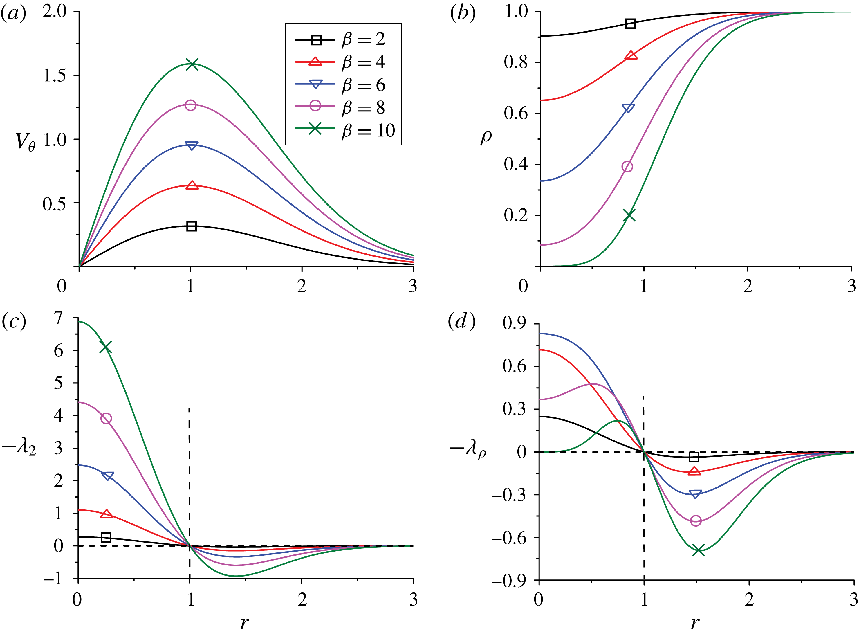
Isentropic Euler vortex: (a) azimuthal velocity; (b) density; (c)
 $-\unicode[STIX]{x1D706}_{2}$
profiles; (d)
 $-\unicode[STIX]{x1D706}_{\unicode[STIX]{x1D70C}}$
profiles for different
 $\unicode[STIX]{x1D6FD}$
values.
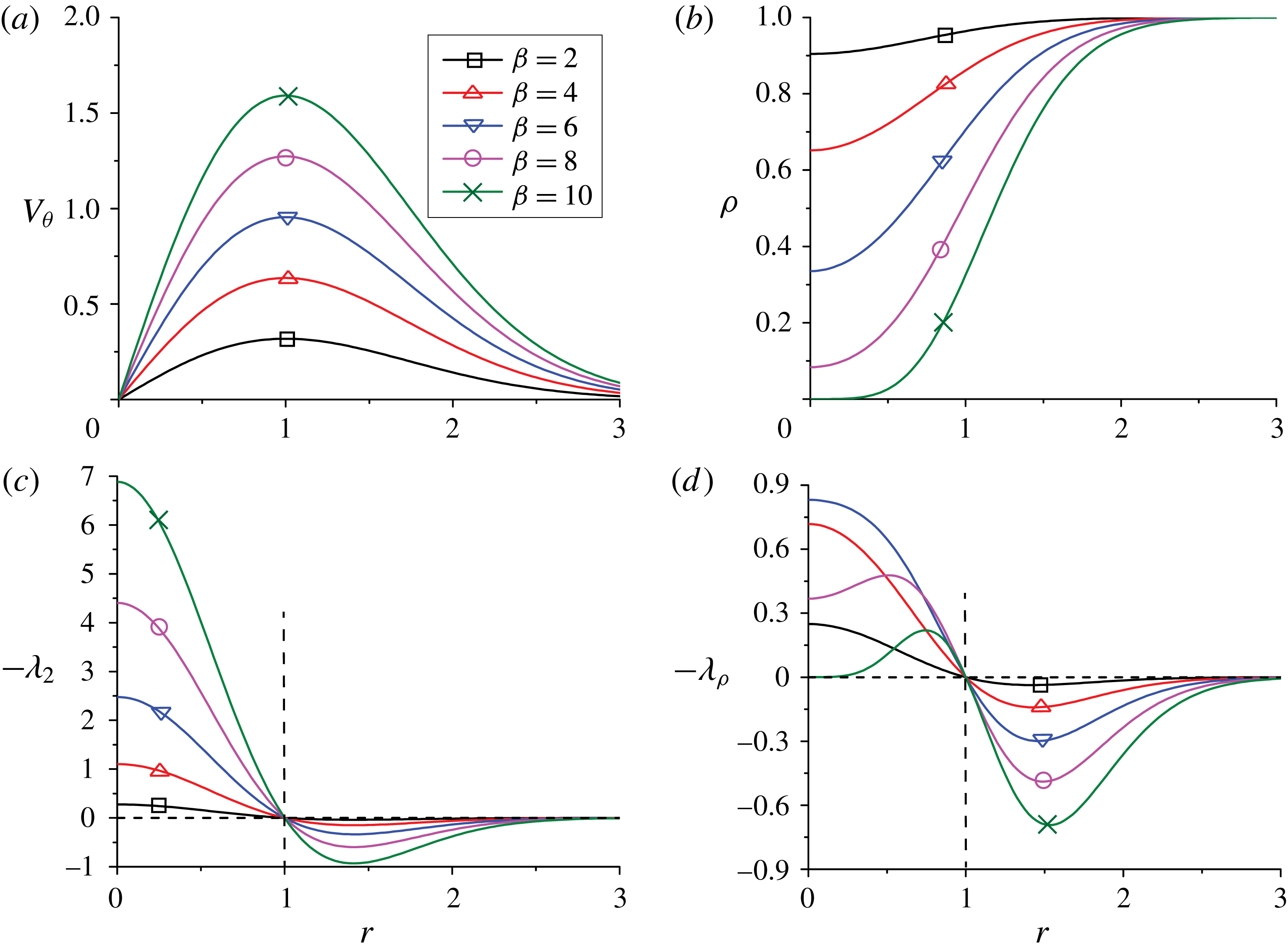
Figures 1(a) and 1(b) display the azimuthal velocity and density profiles for the isentropic vortex with different
 $\unicode[STIX]{x1D6FD}$
values. Figures 1(c) and 1(d) show the corresponding
 $-\unicode[STIX]{x1D706}_{2}$
and
 $-\unicode[STIX]{x1D706}_{\unicode[STIX]{x1D70C}}$
profiles. Note that
 $\unicode[STIX]{x1D70C}^{\prime }$
is positive for this flow, and the vortex core for both
 $\unicode[STIX]{x1D706}_{2}$
and
 $\unicode[STIX]{x1D706}_{\unicode[STIX]{x1D70C}}$
criteria is fixed for all
 $\unicode[STIX]{x1D6FD}$
and is the region bounded by maximum azimuthal velocity (
 $r\leqslant 1$
). The intensity of
 $\unicode[STIX]{x1D706}_{2}$
, which is typically characterized by the magnitude of
 $\unicode[STIX]{x1D706}_{2}$
, increases monotonically with
 $\unicode[STIX]{x1D6FD}$
, i.e. with increasing the angular velocity
 $u_{\unicode[STIX]{x1D703}}/r$
, For a low
 $\unicode[STIX]{x1D6FD}$
case, the
 $\unicode[STIX]{x1D706}_{\unicode[STIX]{x1D70C}}$
and
 $\unicode[STIX]{x1D706}_{2}$
profiles are almost identical, because of small density variation. However, as
 $\unicode[STIX]{x1D6FD}$
increases, the intensity of
 $\unicode[STIX]{x1D706}_{\unicode[STIX]{x1D70C}}$
decreases, especially near the centre, due to decreased density and fluid momentum. Note that for
 $\unicode[STIX]{x1D6FD}\geqslant 10$
, a nonzero threshold will denote a hollow vortex; in such cases, the hollow core should be discarded.
3.2 Liquid jet breakup
Consider a planar liquid jet breakup in a co-flowing gas at the time of ligament formation simulated in Zandian, Sirignano & Hussain (Reference Zandian, Sirignano and Hussain2018), where the gas-to-liquid density ratio
 $\hat{\unicode[STIX]{x1D70C}}=0.1$
and the gas-to-liquid viscosity ratio
 $\hat{\unicode[STIX]{x1D707}}=0.0022$
. Since the flow is incompressible in each phase, the
 $\unicode[STIX]{x1D706}_{\unicode[STIX]{x1D70C}}$
definition is equivalent to the
 $\bar{\unicode[STIX]{x1D706}}_{2}$
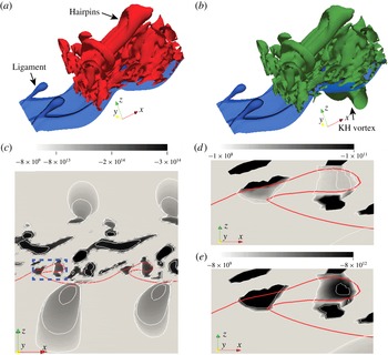
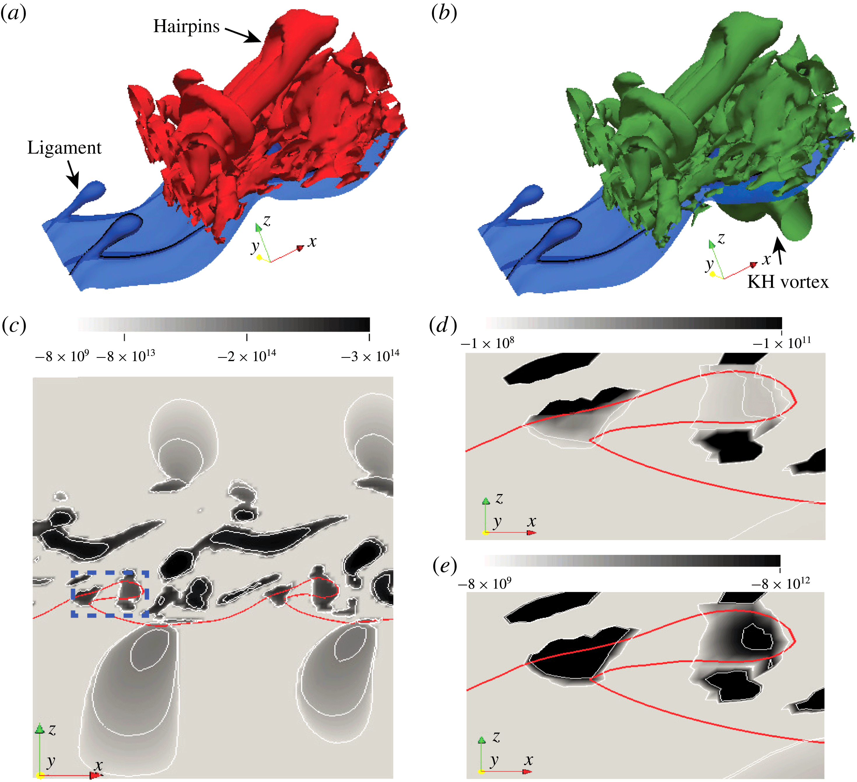
definition away from the interface. Typically, in order to clearly visualize vortical structures, a non-zero threshold is used to suppress noise and very weak or dynamically insignificant structures. Figures 2(a) and 2(b) show
 $\unicode[STIX]{x1D706}_{2}$
and
 $\unicode[STIX]{x1D706}_{\unicode[STIX]{x1D70C}}$
structures, respectively (to match the gas phase vortex structures between (a) and (b), the ratio of threshold of
 $\unicode[STIX]{x1D706}_{\unicode[STIX]{x1D70C}}$
and
 $\unicode[STIX]{x1D706}_{2}$
is set equal to the gas density). Generally, the vortex is much stronger in the gas phase as vorticity diffuses slower due to smaller gas viscosity. In the gas phase, the two definitions produce identical hairpin vortex structures. However,
 $\unicode[STIX]{x1D706}_{\unicode[STIX]{x1D70C}}$
enhances the intensity of vortices in the liquid phase, due to its higher density. In figure 2(b), besides the strong hairpin vortices in the gas phase, the Kelvin–Helmholtz vortex in the liquid phase is captured by the
 $\unicode[STIX]{x1D706}_{\unicode[STIX]{x1D70C}}$
method. Figure 2(c) shows the
 $\unicode[STIX]{x1D706}_{\unicode[STIX]{x1D70C}}$
structure contours on the spanwise section (
 $x$
–
 $z$
plane) cutting through a ligament. Vortex dynamics associated with ligaments is central to understanding atomization (Zandian et al.
Reference Zandian, Sirignano and Hussain2018). Figures 2(d) and 2(e) compare
 $\unicode[STIX]{x1D706}_{2}$
and
 $\unicode[STIX]{x1D706}_{\unicode[STIX]{x1D70C}}$
structures near the ligaments. Since the momentum
 $\unicode[STIX]{x1D70C}\unicode[STIX]{x1D66A}$
is conserved across the interface and gas-to-liquid density ratio
 $\hat{\unicode[STIX]{x1D70C}}=0.1$
, the velocity in the liquid phase is approximately an order of magnitude smaller than in the gas phase. Hence, the vortex structures in the liquid phase based on
 $\unicode[STIX]{x1D706}_{2}$
are much weaker than those in the gas phase and are barely visible. However, using the
 $\unicode[STIX]{x1D706}_{\unicode[STIX]{x1D70C}}$
definition, the intensity of the
 $\unicode[STIX]{x1D706}_{\unicode[STIX]{x1D70C}}$
structures in the ligament is enhanced. Hence,
 $\unicode[STIX]{x1D706}_{\unicode[STIX]{x1D70C}}$
is more suitable for studying the dynamics of ligament and droplet formation.
Liquid jet breakup: (a)
 $\unicode[STIX]{x1D706}_{2}$
(red) and (b)
 $\unicode[STIX]{x1D706}_{\unicode[STIX]{x1D70C}}$
(green) structures with blue denoting the liquid–gas interface; (c)
 $\unicode[STIX]{x1D706}_{\unicode[STIX]{x1D70C}}$
contours on the spanwise cross-section; and detailed comparison between (d)
 $\unicode[STIX]{x1D706}_{2}$
and (e)
 $\unicode[STIX]{x1D706}_{\unicode[STIX]{x1D70C}}$
contours near the ligament (the boxed region in (c)).
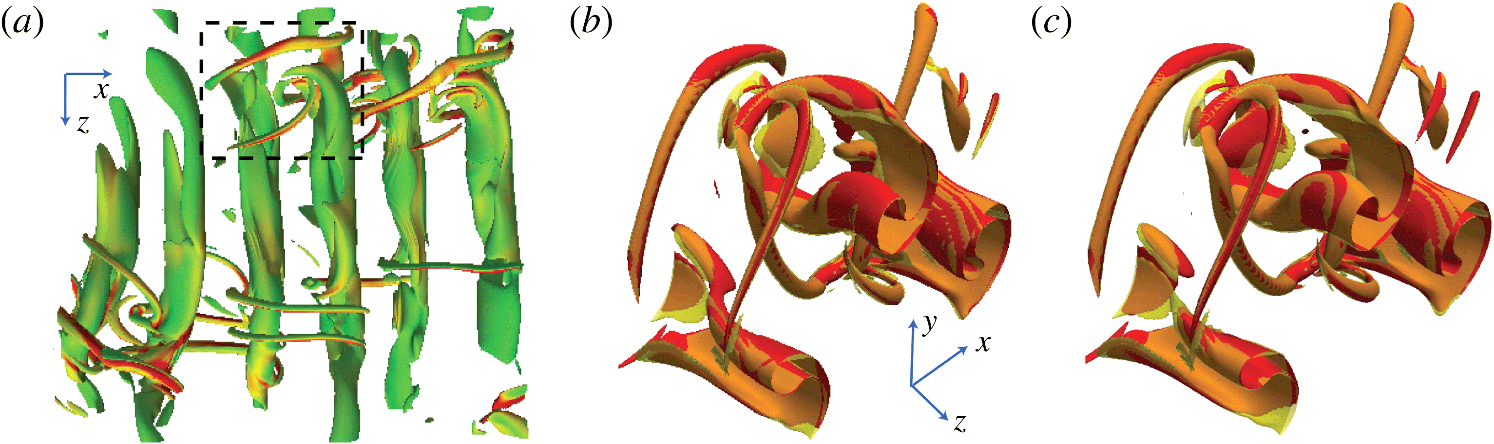
3.3 Compressible wake
 $\unicode[STIX]{x1D706}_{\unicode[STIX]{x1D70C}}$
structures for a high-speed planar wake at free stream
 $M=2$
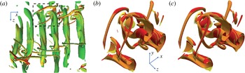
(Hickey, Hussain & Wu Reference Hickey, Hussain and Wu2016) is shown in figure 3(a). As we can see,
 $\unicode[STIX]{x1D706}_{\unicode[STIX]{x1D70C}}$
captures both the roll and rib structures clearly. Figure 3(b) is the detailed comparison of the
 $\unicode[STIX]{x1D706}_{2}$
and
 $\unicode[STIX]{x1D706}_{\unicode[STIX]{x1D70C}}$
vortex structures in the boxed region in figure 3(a). Since the compressibility is weak (turbulent Mach number
 ${<}0.3$
), the
 $\unicode[STIX]{x1D706}_{2}$
and
 $\unicode[STIX]{x1D706}_{\unicode[STIX]{x1D70C}}$
structures almost coincide. Thus, the
 $\unicode[STIX]{x1D706}_{2}$
criterion is still a good approximation of
 $\unicode[STIX]{x1D706}_{\unicode[STIX]{x1D70C}}$
for low
 $M$
compressible flows. To compare with other vortex identification methods, figure 3(c) further shows the structures identified with the
 $\unicode[STIX]{x1D706}_{\unicode[STIX]{x1D70C}}$
and
 $\unicode[STIX]{x1D706}_{ci}$
criteria, the latter is calculated based on the traceless velocity gradient (Pirozzoli et al.
Reference Pirozzoli, Bernardini and Grasso2008). As expected, for this low
 $M$
flow, a very good congruence between
 $\unicode[STIX]{x1D706}_{\unicode[STIX]{x1D70C}}$
and
 $\unicode[STIX]{x1D706}_{ci}$
is also observed.
Compressible wake: (a)
 $\unicode[STIX]{x1D706}_{\unicode[STIX]{x1D70C}}$
structures coloured by vorticity magnitude; detailed comparison between (b)
 $\unicode[STIX]{x1D706}_{2}$
(red) and
 $\unicode[STIX]{x1D706}_{\unicode[STIX]{x1D70C}}$
(brown) structures; (c)
 $\unicode[STIX]{x1D706}_{ci}$
(red) and
 $\unicode[STIX]{x1D706}_{\unicode[STIX]{x1D70C}}$
(brown) structures in the boxed region marked in (a).
3.4 Compressible turbulent channel flows
Direct numerical simulation (DNS) datasets of compressible turbulent channel flows with
 $M=0.8$
,
 $2$
and
 $3$
at bulk Reynolds number
 $Re_{b}=3000$
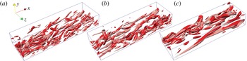
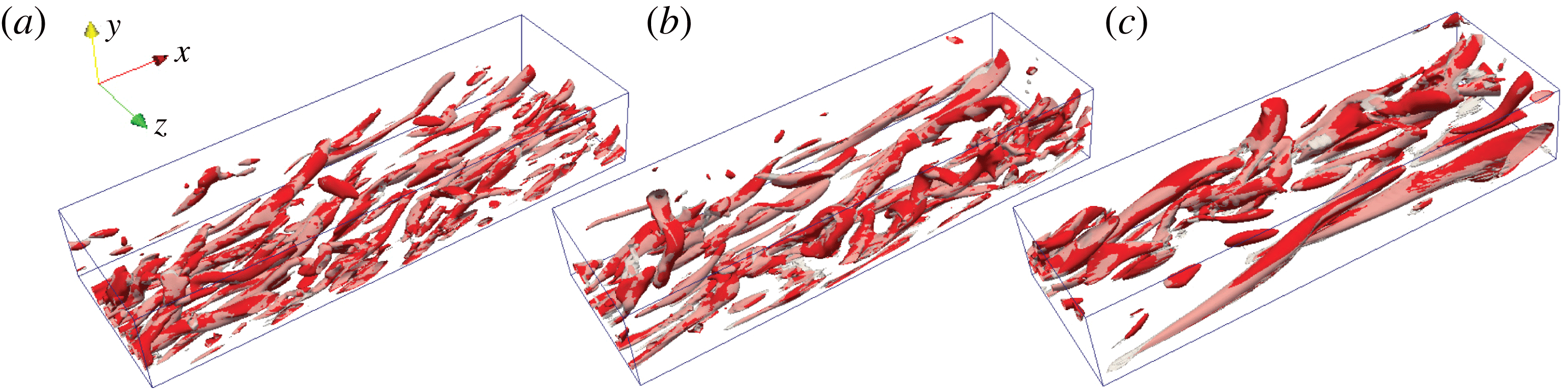
are considered here. Figure 4 compares
 $\unicode[STIX]{x1D706}_{\unicode[STIX]{x1D70C}}$
and
 $\unicode[STIX]{x1D706}_{2}$
structures in the bottom half of the channel (the threshold is chosen as the root-mean-square (r.m.s.) value of each criterion at each
 $M$
). Note that since the
 $\unicode[STIX]{x1D706}_{ci}$
agrees well with the
 $\unicode[STIX]{x1D706}_{2}$
criterion for all these cases, here, only the
 $\unicode[STIX]{x1D706}_{2}$
structures are compared. As
 $M$
increases, the structures are more sparsely distributed and elongated, possibly due to higher shear at higher
 $M$
. For
 $M$
up to
 $3$
, the
 $\unicode[STIX]{x1D706}_{2}$
and
 $\unicode[STIX]{x1D706}_{\unicode[STIX]{x1D70C}}$
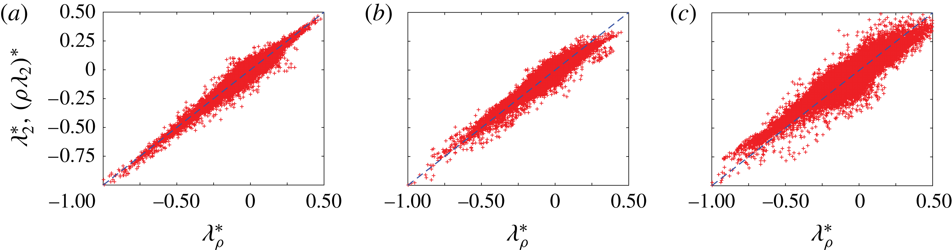
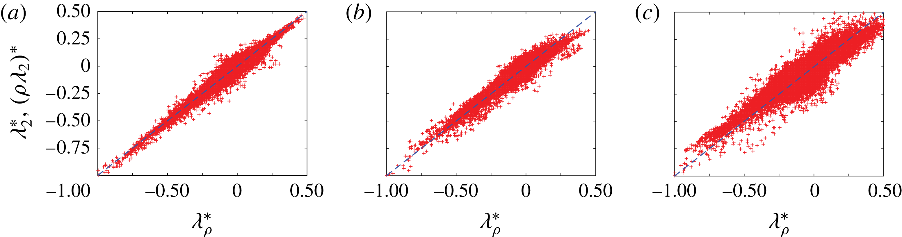
structures still coincide. The scatter plot of
 $\unicode[STIX]{x1D706}_{\unicode[STIX]{x1D70C}}$
against
 $\unicode[STIX]{x1D706}_{2}$
is shown in figure 5. As expected, the
 $\unicode[STIX]{x1D706}_{\unicode[STIX]{x1D70C}}$
and
 $\unicode[STIX]{x1D706}_{2}$
structures show a relatively strong correlation: for
 $M=0.8$
, if
 $\unicode[STIX]{x1D706}_{\unicode[STIX]{x1D70C}}$
is high, so is
 $\unicode[STIX]{x1D706}_{2}$
; this correlation is reduced at
 $M=3$
, indicating that the
 $\unicode[STIX]{x1D706}_{2}$
and
 $\unicode[STIX]{x1D706}_{\unicode[STIX]{x1D70C}}$
structures would differ more for higher
 $M$
flows.
Compressible turbulent channel: comparison of
 $\unicode[STIX]{x1D706}_{2}$
(red) and
 $\unicode[STIX]{x1D706}_{\unicode[STIX]{x1D70C}}$
(grey) structures at (a)
 $M=0.8$
; (b)
 $M=2$
; and (c)
 $M=3$
.
Scatter plots of normalized
 $\unicode[STIX]{x1D706}_{\unicode[STIX]{x1D70C}}$
against
 $\unicode[STIX]{x1D706}_{2}$
for compressible turbulent channel flows at (a)
 $M=0.8$
; (b)
 $M=2$
; and (c)
 $M=3$
. The quantities are normalized by their maximum values, and the dashed line denotes
 $\unicode[STIX]{x1D706}_{\unicode[STIX]{x1D70C}}/\max (|\unicode[STIX]{x1D706}_{\unicode[STIX]{x1D70C}}|)=\unicode[STIX]{x1D706}_{2}/\max (|\unicode[STIX]{x1D706}_{2}|)$
.
3.5 Hypersonic boundary layers
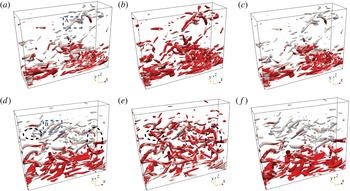
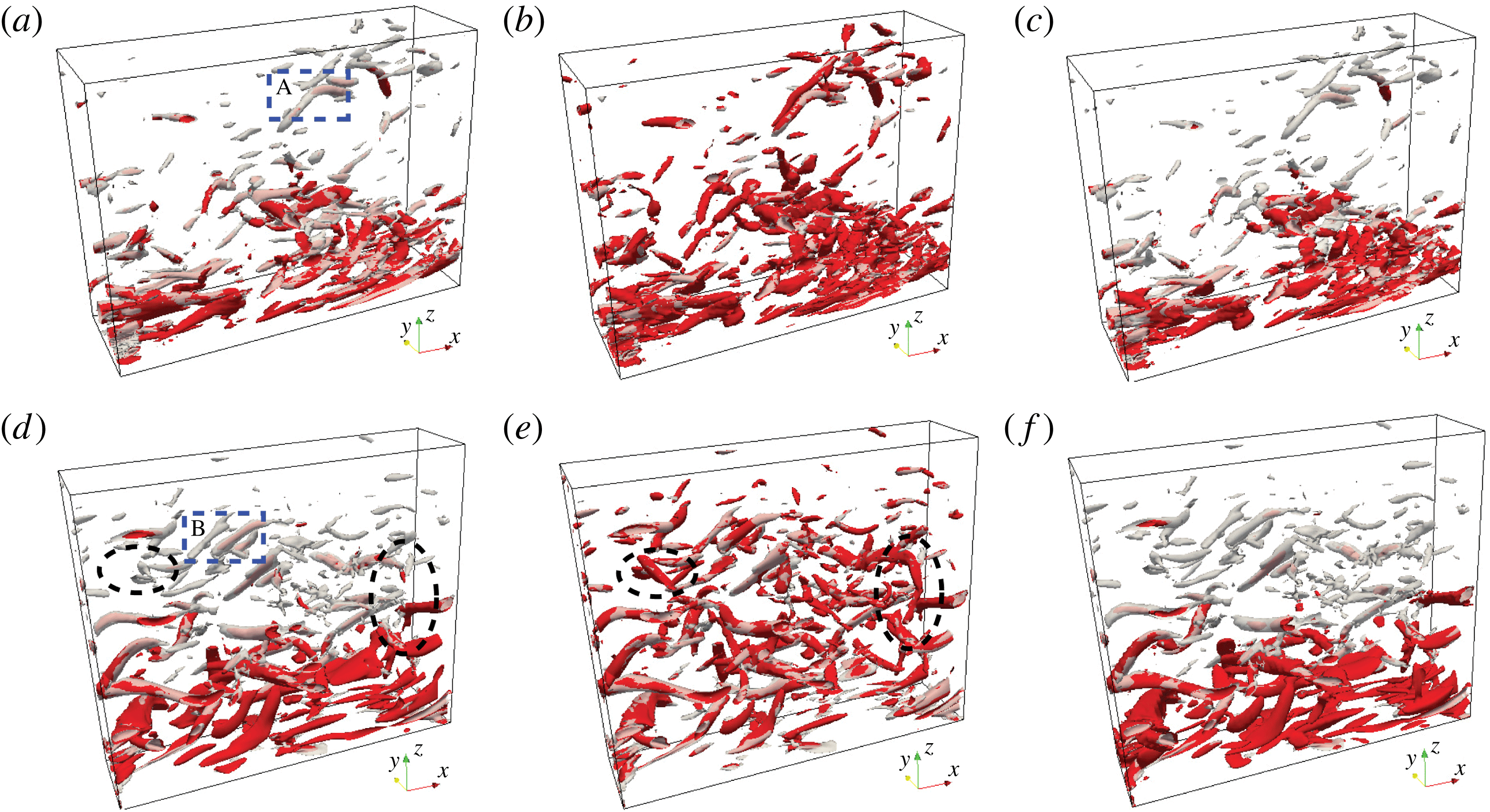
As a final example, we consider the zero-pressure-gradient hypersonic turbulent boundary layer, which involves strong density variation in the wall-normal direction (for simulation details see Duan, Choudhari & Zhang (Reference Duan, Choudhari and Zhang2016); Zhang, Duan & Choudhari (Reference Zhang, Duan and Choudhari2016)). Figure 6(a) compares
 $\unicode[STIX]{x1D706}_{2}$
and
 $\unicode[STIX]{x1D706}_{\unicode[STIX]{x1D70C}}$
structures at
 $M=6$
(the threshold is chosen as twice the r.m.s. value of each criterion). The
 $\unicode[STIX]{x1D706}_{2}$
structures are located nearer to the wall, and are akin to the typical streamwise vortices observed in subsonic and supersonic boundary layers. As for
 $\unicode[STIX]{x1D706}_{\unicode[STIX]{x1D70C}}$
, in addition to the near-wall structures, numerous coherent structures are captured far away from the wall. Figures 6(b) and 6(c) further compare structures of
 $\unicode[STIX]{x1D706}_{\unicode[STIX]{x1D70C}}$
with
 $\bar{\unicode[STIX]{x1D706}}_{2}$
and
 $\unicode[STIX]{x1D706}_{ci}$
, respectively. For this moderate
 $M$
(
 $=6$
) hypersonic flow, the
 $\bar{\unicode[STIX]{x1D706}}_{2}$
structures closely match the
 $\unicode[STIX]{x1D706}_{\unicode[STIX]{x1D70C}}$
structures. The
 $\unicode[STIX]{x1D706}_{ci}$
structures, which seem to be quite similar to those of
 $\unicode[STIX]{x1D706}_{2}$
, differ from the
 $\unicode[STIX]{x1D706}_{\unicode[STIX]{x1D70C}}$
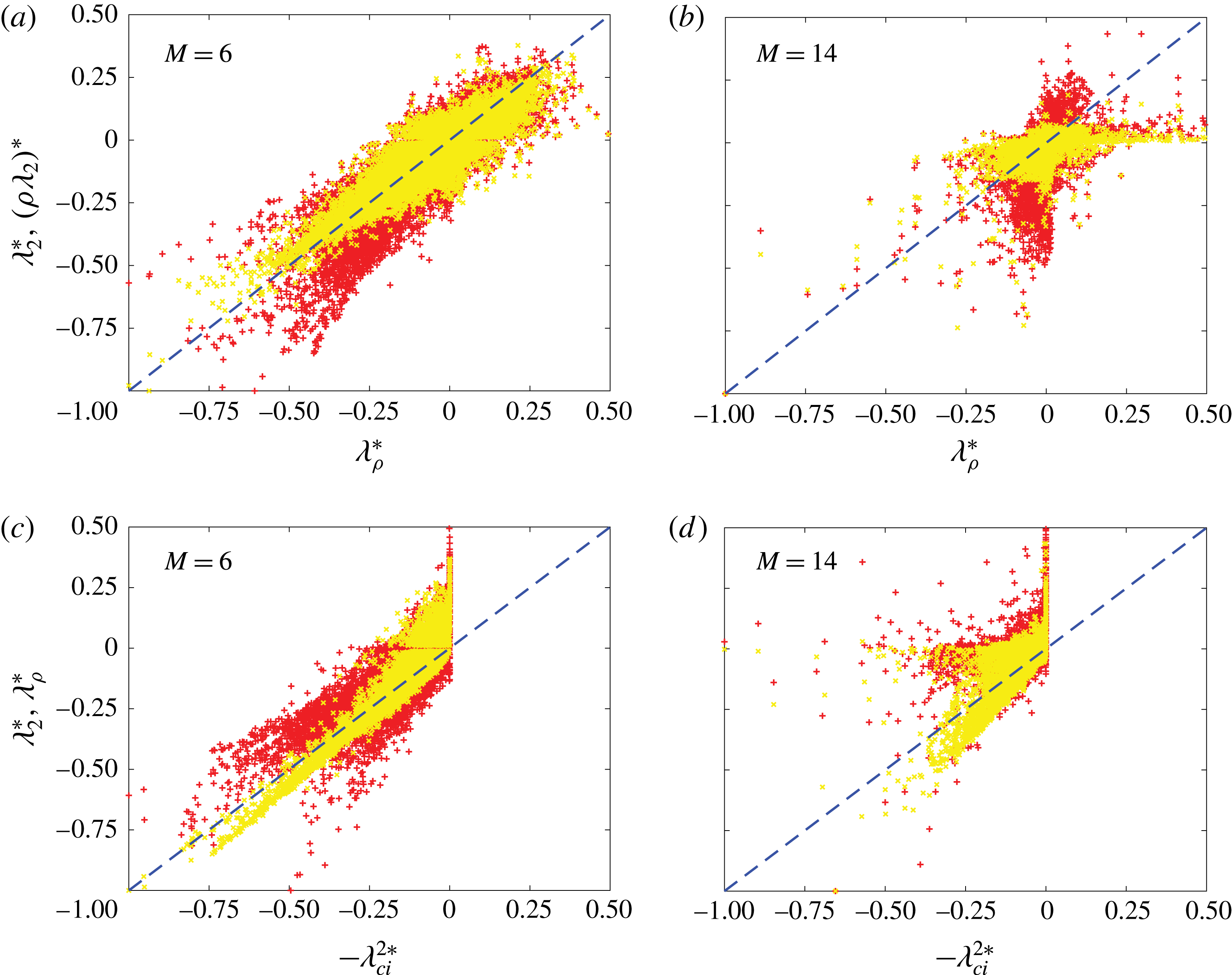
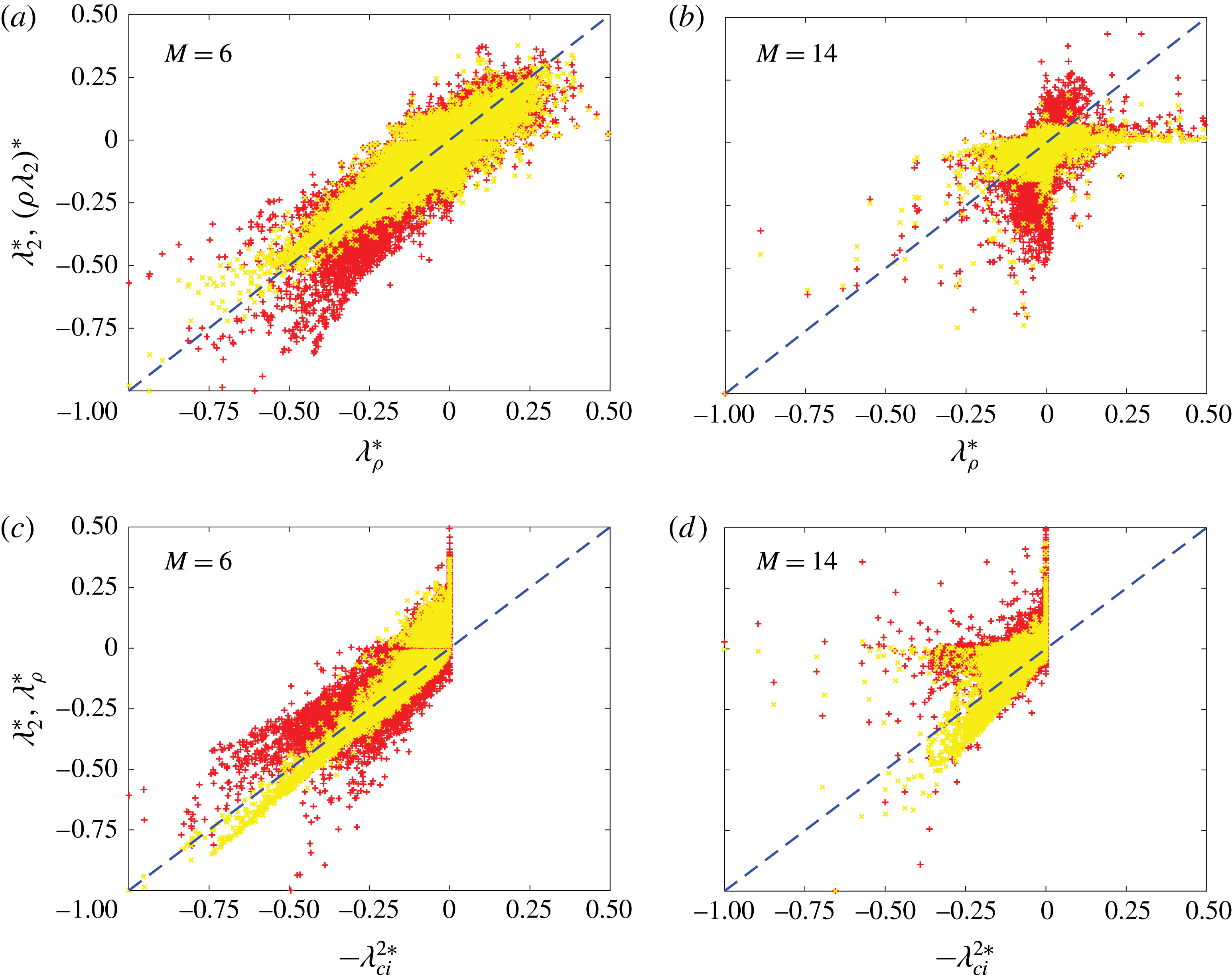
structures mainly in the outer region of the boundary layer. These observations are further confirmed by the scatter plots. In figure 7(a), both the red (
 $\unicode[STIX]{x1D706}_{\unicode[STIX]{x1D70C}}$
and
 $\unicode[STIX]{x1D706}_{2}$
) and yellow (
 $\unicode[STIX]{x1D706}_{\unicode[STIX]{x1D70C}}$
and
 $\bar{\unicode[STIX]{x1D706}}_{2}$
) data points are mostly located along the
 $45^{\circ }$
line; however, the yellow data points are more compact, indicating closer similarity between
 $\unicode[STIX]{x1D706}_{\unicode[STIX]{x1D70C}}$
and
 $\bar{\unicode[STIX]{x1D706}}_{2}$
than between
 $\unicode[STIX]{x1D706}_{\unicode[STIX]{x1D70C}}$
and
 $\unicode[STIX]{x1D706}_{2}$
. Surprisingly, for hypersonic flow at this
 $M=6$
, the
 $\unicode[STIX]{x1D706}_{2}$
is still well correlated with
 $-\unicode[STIX]{x1D706}_{ci}^{2}$
(figure 7
c), indicating that the dilatation effect is not significant (note that,
 $\unicode[STIX]{x1D706}_{ci}^{2}$
is employed here for dimensional consistency with
 $\unicode[STIX]{x1D706}_{2}$
). For
 $M=14$
, the difference between
 $\unicode[STIX]{x1D706}_{2}$
and
 $\unicode[STIX]{x1D706}_{\unicode[STIX]{x1D70C}}$
structures becomes even larger. Although
 $\bar{\unicode[STIX]{x1D706}}_{2}$
is still a good approximation of
 $\unicode[STIX]{x1D706}_{\unicode[STIX]{x1D70C}}$
, the disparity becomes more pronounced (see the circled region of figure 6
d,e), showing the enhanced effects of density variation and dilatation at high
 $M$
. The scatter plot in figure 7(b) also shows that even
 $\bar{\unicode[STIX]{x1D706}}_{2}$
and
 $\unicode[STIX]{x1D706}_{\unicode[STIX]{x1D70C}}$
are less correlated for this high
 $M$
case. In addition, figure 7(d) shows that the difference between
 $\unicode[STIX]{x1D706}_{ci}$
and
 $\unicode[STIX]{x1D706}_{\unicode[STIX]{x1D70C}}$
(as also between
 $\unicode[STIX]{x1D706}_{ci}$
and
 $\unicode[STIX]{x1D706}_{2}$
) becomes larger at this high
 $M$
; this is clearly expected from the structure comparison shown in figure 6(f). Interestingly,
 $\unicode[STIX]{x1D706}_{\unicode[STIX]{x1D70C}}$
(also
 $\unicode[STIX]{x1D706}_{2}$
) is almost around zero for the point where
 $\unicode[STIX]{x1D706}_{ci}$
is maximum. This discrepancy needs to be further investigated.
Hypersonic boundary layers: comparison of (a,d)
 $\unicode[STIX]{x1D706}_{\unicode[STIX]{x1D70C}}$
(grey) and
 $\unicode[STIX]{x1D706}_{2}$
(red) structures; (b,e)
 $\unicode[STIX]{x1D706}_{\unicode[STIX]{x1D70C}}$
(grey) and
 $\bar{\unicode[STIX]{x1D706}}_{2}$
(red) structures; (c,f)
 $\unicode[STIX]{x1D706}_{\unicode[STIX]{x1D70C}}$
(grey) and
 $\bar{\unicode[STIX]{x1D706}}_{ci}$
(red) structures for (a–c)
 $M=6$
and (d–f)
 $M=14$
. Regions marked as A and B relate to later discussions of figure 8.
Scatter plots: (a,b)
 $\unicode[STIX]{x1D706}_{\unicode[STIX]{x1D70C}}$
against
 $\unicode[STIX]{x1D706}_{2}$
(red,
 $+$
) and
 $\bar{\unicode[STIX]{x1D706}}_{2}$
(yellow,
 $^{\ast }$
); and (c,d)
 $-\unicode[STIX]{x1D706}_{ci}^{2}$
against
 $\unicode[STIX]{x1D706}_{\unicode[STIX]{x1D70C}}$
(red) and
 $\unicode[STIX]{x1D706}_{2}$
(yellow) for hypersonic turbulent boundary layers at (a,c)
 $M=6$
; (b,d)
 $M=14$
.
Generally, for hypersonic flows,
 $\unicode[STIX]{x1D706}_{\unicode[STIX]{x1D70C}}$
captures more dynamical coherent structures than the other criteria, i.e.
 $\unicode[STIX]{x1D706}_{2}$
and
 $\unicode[STIX]{x1D706}_{ci}$
. An interesting question arises as to whether these additional
 $\unicode[STIX]{x1D706}_{\unicode[STIX]{x1D70C}}$
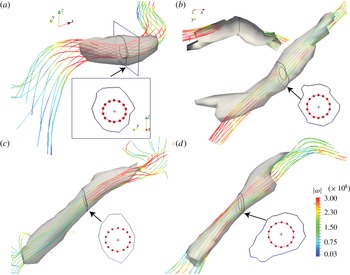
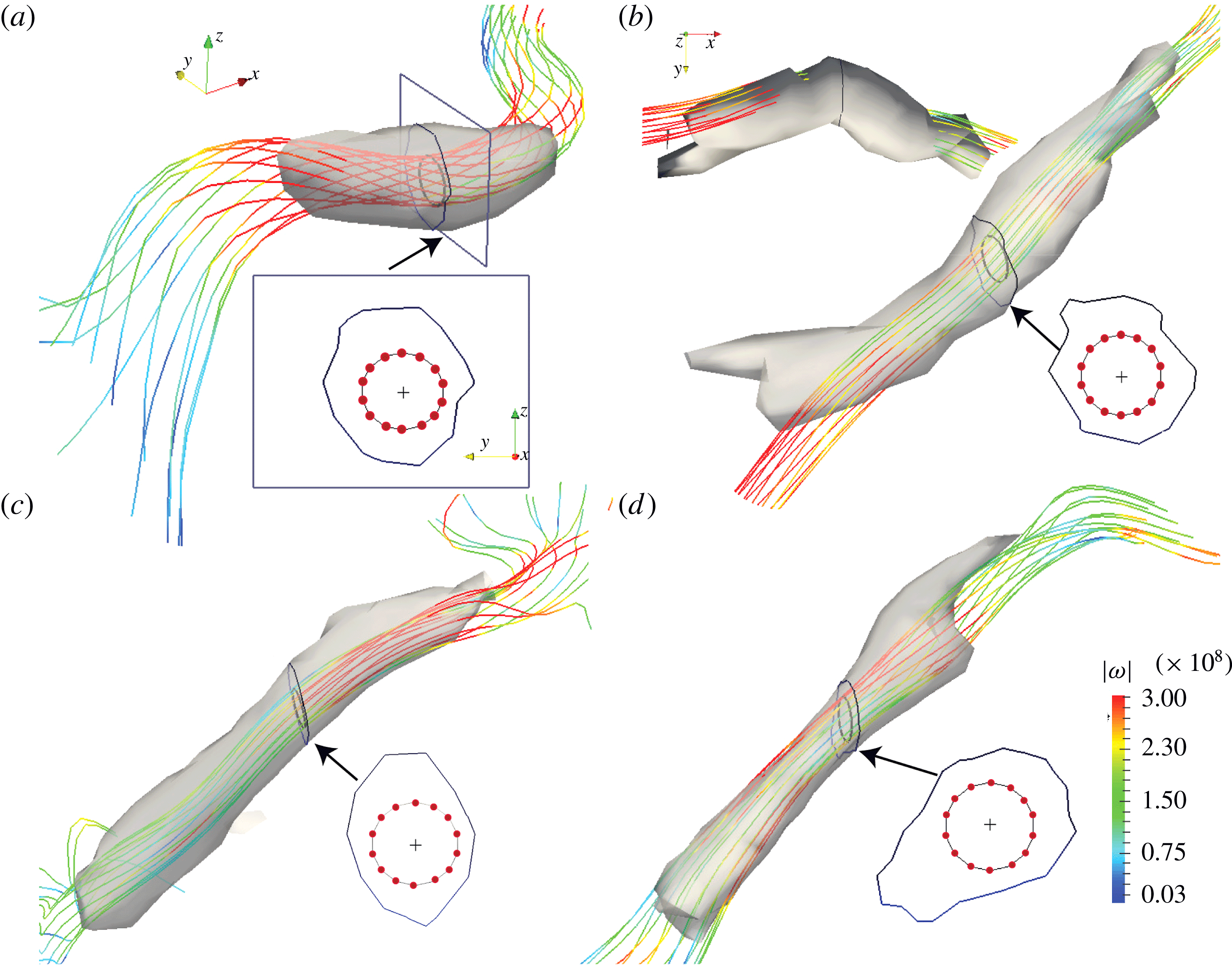
structures satisfy the basic requirement of vortices – namely, compact regions with high vorticity. To this end, figure 8 further shows the zoomed-in view of the
 $\unicode[STIX]{x1D706}_{\unicode[STIX]{x1D70C}}$
structures in the outer boundary layer region along with vorticity lines for the
 $M=6$
and
 $14$
cases (marked as regions A and B in figure 6
a,d). For each
 $M$
, one
 $\unicode[STIX]{x1D706}_{\unicode[STIX]{x1D70C}}$
structure (figure 8
a,c) is a
 $\unicode[STIX]{x1D706}_{2}$
structure also, and the other one (figure 8
a,c) is only a
 $\unicode[STIX]{x1D706}_{\unicode[STIX]{x1D70C}}$
structure. Note that all vorticity lines originate from the points, which are equally distributed on a circle centred at the
 $-\unicode[STIX]{x1D706}_{\unicode[STIX]{x1D70C}}$
peak in each structure marked as the
 $+$
sign shown in the cross-sectional view, and then are extended in both directions away from this cross-section. The vorticity lines, generally along the
 $\unicode[STIX]{x1D706}_{\unicode[STIX]{x1D70C}}$
structures, can also deviate from the vortical structures (as clearly shown in figure 8
b). This observation that vorticity lines originating from the structure core do not necessarily remain within the core but can cross the structure surface – contrary to popular belief – was also noted by Jeong et al. (Reference Jeong, Hussain, Schoppa and Kim1997) and Schoppa & Hussain (Reference Schoppa and Hussain2002) in their studies of coherent structures in incompressible turbulent channel flows. Note that all
 $\unicode[STIX]{x1D706}_{\unicode[STIX]{x1D70C}}$
structures, whether coinciding with
 $\unicode[STIX]{x1D706}_{2}$
structures or not, are associated with relatively high vorticity concentrated on a collection of extended vortex lines. Therefore, the structures in the outer boundary layer region revealed by
 $\unicode[STIX]{x1D706}_{\unicode[STIX]{x1D70C}}$
, although not necessarily by
 $\unicode[STIX]{x1D706}_{2}$
, are indeed vortices. How important these new-found structures are in the flow dynamics needs further study.
Zoomed-in view of the
 $\unicode[STIX]{x1D706}_{\unicode[STIX]{x1D70C}}$
structures marked in the boxed regions (A,B) in figure 6 along with vorticity lines shaded by vorticity magnitude for (a,b)
 $M=6$
and (c,d)
 $M=14$
. Note that the structures in (a,c) are
 $\unicode[STIX]{x1D706}_{2}$
structures also, and (b,d) are
 $\unicode[STIX]{x1D706}_{\unicode[STIX]{x1D70C}}$
structures only. The seeding points (red dots) for the vorticity lines are shown in the cross-sectional view with
 $+$
indicating
 $-\unicode[STIX]{x1D706}_{\unicode[STIX]{x1D70C}}$
peak in each structure.
Recall that although vortices are associated with high vorticity, the reverse is not true; namely, high vorticity regions are not necessarily vortices (Dubief & Delcayre Reference Dubief and Delcayre2000; Günther & Theisel Reference Günther and Theisel2017, JH). For example, the laminar pipe flow has high vorticity near the wall but has no vortex. Hence, the
 $\unicode[STIX]{x1D706}_{\unicode[STIX]{x1D70C}}$
and
 $\unicode[STIX]{x1D706}_{2}$
(as well as
 $Q$
,
 $\unicode[STIX]{x1D6E5}$
and
 $\unicode[STIX]{x1D706}_{ci}$
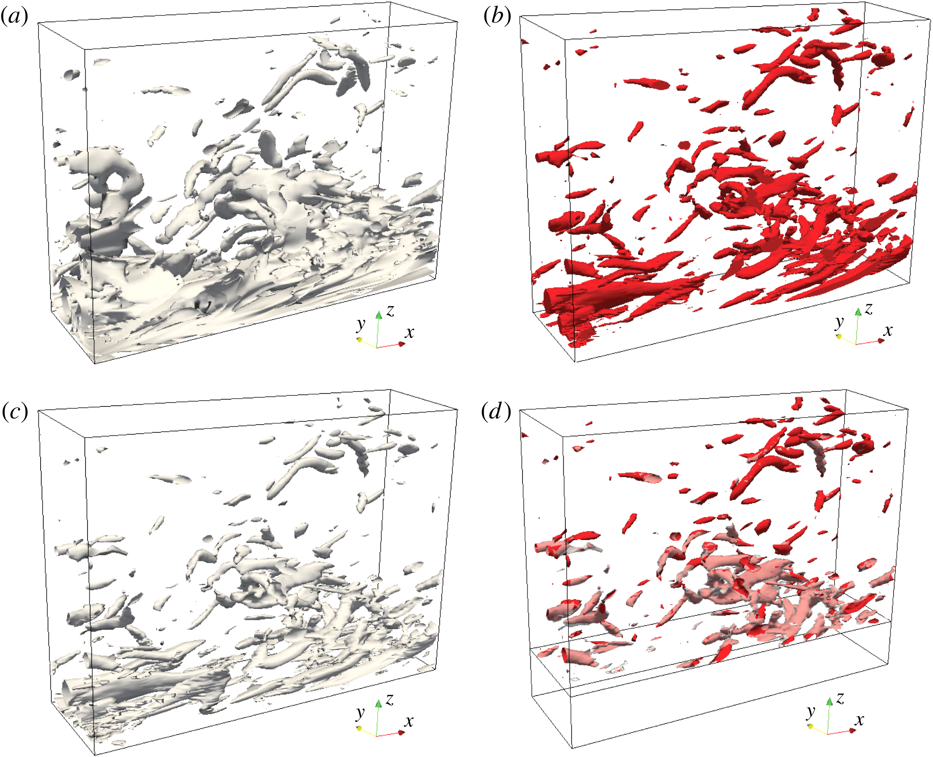
, etc.) criteria are meant to identify vortices (with compact cross-sections), but not all regions of high vorticity, such as vorticity sheets or near-wall shear layers for wall-bounded flows. As an example, in figure 9 we further compare the iso-surfaces of: (a) vorticity magnitude
 $|\unicode[STIX]{x1D74E}|$
; (b)
 $\unicode[STIX]{x1D706}_{\unicode[STIX]{x1D70C}}$
; (c)
 $\unicode[STIX]{x1D706}_{\unicode[STIX]{x1D70C}}|\unicode[STIX]{x1D74E}|$
, indicating correlation between
 $\unicode[STIX]{x1D706}_{\unicode[STIX]{x1D70C}}$
and
 $|\unicode[STIX]{x1D74E}|$
; and superimposed iso-surfaces of both
 $\unicode[STIX]{x1D706}_{\unicode[STIX]{x1D70C}}$
and
 $\unicode[STIX]{x1D706}_{\unicode[STIX]{x1D70C}}|\unicode[STIX]{x1D74E}|$
from figures 9(b) and 9(c) excluding the near-wall region for the
 $M=6$
hypersonic turbulent boundary layer; the same data as shown in figure 6. Note that the structure surfaces of
 $|\unicode[STIX]{x1D74E}|$
,
 $\unicode[STIX]{x1D706}_{\unicode[STIX]{x1D70C}}$
and
 $\unicode[STIX]{x1D706}_{\unicode[STIX]{x1D70C}}|\unicode[STIX]{x1D74E}|$
in figure 9 are plotted with the thresholds of
 $0.5$
,
 $1.0$
and
 $2.0$
times their own r.m.s. values in the domain, respectively; choices of these thresholds make the structures in the different figures of comparable sizes. Figure 9(b) shows that
 $\unicode[STIX]{x1D706}_{\unicode[STIX]{x1D70C}}$
successfully identifies vortices with high vorticity in the outer region but excludes other regions of high vorticity like sheets in the near-wall region (included in figure 9
a); that is,
 $\unicode[STIX]{x1D706}_{\unicode[STIX]{x1D70C}}$
does not identify all regions of high vorticity but only vortices (which are associated with high vorticity and are compact). Clearly, therefore, high correlation between
 $\unicode[STIX]{x1D706}_{\unicode[STIX]{x1D70C}}$
and
 $|\unicode[STIX]{x1D74E}|$
does not always represent vortices uniquely as it can also highlight regions with high vorticity but not vortices. This is why the structures near the wall in figure 9(c) are not identical to those in figure 9(b); but, indeed, there is good correlation between
 $\unicode[STIX]{x1D706}_{\unicode[STIX]{x1D70C}}$
and
 $|\unicode[STIX]{x1D74E}|$
sufficiently away from the wall (figure 9
d), where the background shear is relatively weak.
Iso-surfaces of (a) vorticity magnitude
 $|\unicode[STIX]{x1D74E}|$
; (b)
 $\unicode[STIX]{x1D706}_{\unicode[STIX]{x1D70C}}$
; (c)
 $\unicode[STIX]{x1D706}_{\unicode[STIX]{x1D70C}}|\unicode[STIX]{x1D74E}|$
; and (d) superimposition of (b) and (c) in the outer region for the
 $M=6$
hypersonic turbulent boundary layer shown in figure 6.
4 Conclusion
In summary, we present a new dynamical vortex definition for flows with a variable density effect, such as compressible and multi-phase flows. This new
 $\unicode[STIX]{x1D706}_{\unicode[STIX]{x1D70C}}$
criterion, which is derived directly from the compressible momentum (N–S) equation, identifies the coherent local pressure minimum in a plane. Employing the analytically derived characteristics of the axisymmetric isentropic Euler vortex, we demonstrate that
 $\unicode[STIX]{x1D706}_{\unicode[STIX]{x1D70C}}$
can better characterize the pressure Hessian than the kinematic criteria for variable density flows.
 $\unicode[STIX]{x1D706}_{\unicode[STIX]{x1D70C}}$
is also examined and compared with the
 $\unicode[STIX]{x1D706}_{2}$
and
 $\unicode[STIX]{x1D706}_{ci}$
for a variety of DNS data. As for the low
 $M$
(i.e.
 ${<}5$
) flows, where the compressibility effect is weak, very good congruence between
 $\unicode[STIX]{x1D706}_{\unicode[STIX]{x1D70C}}$
and
 $\unicode[STIX]{x1D706}_{2}$
(also
 $\unicode[STIX]{x1D706}_{ci}$
) are observed. For multi-phase and moderate hypersonic flows,
 $\bar{\unicode[STIX]{x1D706}}_{2}$
works better than
 $\unicode[STIX]{x1D706}_{2}$
. However, the
 $\unicode[STIX]{x1D706}_{\unicode[STIX]{x1D70C}}$
definition seems to be highly appropriate for studying vortex dynamics and flow control in highly compressible and strongly varying density flows and will be investigated in the future. In addition, it would be interesting to explore the applicability of the new
 $\unicode[STIX]{x1D706}_{\unicode[STIX]{x1D70C}}$
definition for other complicated flows, such as turbulent reacting and supercritical flows (Chakraborty et al.
Reference Chakraborty, Wang, Konstantinou and Klein2017; Kim, Hickey & Scalo Reference Kim, Hickey and Scalo2017). Systematic comparisons with other criteria, such as the average corotation method and
 $Q_{M}$
(Kolář & Šístek Reference Kolář and Šístek2015) are also needed.
Acknowledgements
We are grateful to A. Zandian, W. A. Sirignano, J.-P. Hickey, C. Zhang and L. Duan for providing us their DNS datasets and post-processing codes. We also thank E. Stout and X. Chen for helpful discussions.