2. Preliminaries

Consider the propagation of surface–acoustic wave disturbances in water of constant depth $h$ over a rigid bottom ( $z=-h$ ), due to the combined action of gravity and compressibility. Following Longuet-Higgins (Reference Longuet-Higgins1950), water will be treated as an inviscid barotropic fluid (where the pressure $p$ is a function of the density ${\it\rho}$ only) with constant sound speed $c=(\text{d}p/\text{d}{\it\rho})^{1/2}$ , and the motion will be assumed irrotational.

A key parameter, which controls the effects of compressibility relative to gravity, is

where $g$ is the gravitational acceleration. Typically, this parameter is small ( ${\it\mu}\ll 1$ ), as the sound speed in water, $c=1.5\times 10^{3}~\text{m}~\text{s}^{-1}$ , far exceeds the maximum phase speed of gravity waves $(gh)^{1/2}$ (under oceanic conditions, for $h=150$ – $1500$ m, say, ${\it\mu}\simeq 10^{-3}$ – $10^{-2}$ ). As a result, free-surface (gravity) wave disturbances feature vastly different spatial and/or temporal scales from acoustic (compression) wave modes.

The present study is concerned with nonlinear interactions between gravity and acoustic modes of comparable temporal, but disparate spatial, scales. Specifically, the gravity wavelength ${\it\lambda}$ is much shorter than the acoustic length scale represented by the water depth $({\it\lambda}\ll h)$ , whereas the gravity time scale ${\it\tau}\sim ({\it\lambda}/g)^{1/2}$ in keeping with the deep-water dispersion relation. Then, taking ${\it\tau}$ to be comparable to the acoustic time scale $h/c$ implies ${\it\lambda}\sim {\it\mu}h$ ; hence, in the present setting, the parameter ${\it\mu}$ may be interpreted as the ratio of the gravity length scale to the acoustic length scale.

Based on irrotationality, the surface–acoustic wave problem is formulated in terms of the velocity potential ${\it\varphi}(x,z,t)$ , where $\boldsymbol{u}=\boldsymbol{{\rm\nabla}}{\it\varphi}$ is the velocity field. Moreover, we shall use dimensionless variables, employing ${\it\mu}h$ as length scale and $h/c$ as time scale. As in Longuet-Higgins (Reference Longuet-Higgins1950), the equation governing ${\it\varphi}$ in the fluid interior is obtained by combining continuity with the unsteady Bernoulli equation. Specifically, ${\it\varphi}$ satisfies

In addition, the usual kinematic and dynamic conditions apply on the free surface $z={\it\eta}(x,t)$ . For the purposes of the ensuing weakly nonlinear analysis, it will be sufficient to satisfy these conditions correct up to cubic terms in the perturbations. After expanding the two free-surface conditions about $z=0$ , ${\it\eta}$ may be expressed in terms of ${\it\varphi}$ to this order of approximation. Thus, eliminating ${\it\eta}$ , we arrive at the following boundary condition for ${\it\varphi}$ on $z=0$ :

Finally, the boundary condition on the rigid bottom at $z=-1/{\it\mu}$ reads

In the limit ${\it\mu}\ll 1$ , (2.2) along with the boundary conditions (2.3) reduce to the classical incompressible deep-water-wave problem (correct to cubic terms). This reflects the fact that the chosen length scale ${\it\mu}h$ pertains to deep-water gravity waves, which are confined close to the free surface. Acoustic waves, by contrast, extend through the entire fluid depth, and $x$ and $z$ have to be rescaled accordingly in order to capture these disturbances for ${\it\mu}\ll 1$ .

This disparity in length scales is brought out by the linear propagation modes of a slightly compressible fluid layer with a free surface (Longuet-Higgins Reference Longuet-Higgins1950; Dalrymple & Rogers Reference Dalrymple and Rogers2006). Dropping the nonlinear terms in (2.2) and (2.3a ), we look for wave modes that propagate along $x$ with wavenumber $k$ and frequency ${\it\omega}$ , in the form

Upon substituting (2.4) into (2.2) and (2.3), the vertical profile $f(z)$ satisfies the boundary-value problem

For ${\it\mu}\ll 1$ and $k=O(1)$ , the solution to this problem decays exponentially into the fluid,

and ${\it\omega}$ satisfies the dispersion relation

As expected, to leading order, this recovers the familiar gravity surface wave mode on deep water.

On the other hand, according to (2.5), the vertical profile $f(z)$ becomes oscillatory in the low-wavenumber limit, $k^{2}<{\it\mu}^{2}{\it\omega}^{2}$ . To analyse this possibility, we write

this rescaling amounts to using $h$ instead of ${\it\mu}h$ as the characteristic length scale. Assuming ${\it\Omega}^{2}={\it\omega}^{2}-{\it\kappa}^{2}>0$ , it follows from (2.5) and (2.6), after implementing (2.9), that

where

Solving (2.11) for ${\it\mu}\ll 1$ then reveals a countable infinity of propagation modes that obey the dispersion relations

where ${\it\omega}_{n}=(n+(1/2)){\rm\pi}$ .

To leading order the dispersion relations (2.12) agree with those of pure acoustic waves in a fluid layer bounded by a rigid bottom and a free surface. It should be noted that, unlike the gravity mode (2.7) which is confined close to the free surface $(|Z|\ll 1)$ , the compression modes (2.10) reside in the fluid interior ( $-1<Z<0$ ). Moreover, according to (2.12), each acoustic mode can propagate along $x$ $({\it\kappa}^{2}>0)$ only if ${\it\omega}>{\it\omega}_{n}^{c}$ , where

is the corresponding cutoff frequency.

3. Resonant triads

The strongest nonlinear wave interactions in dispersive systems derive from quadratic terms, and involve particular trios of wavetrains satisfying certain resonance conditions. Such resonant triad interactions, however, are not possible among surface gravity waves (Phillips Reference Phillips1960). On the other hand, allowing for compressibility effects, two gravity waves may interact resonantly with an acoustic wave. Kadri & Stiassnie (Reference Kadri and Stiassnie2013) gave specific examples of such acoustic–gravity triads, from numerical solutions of the triad resonance conditions. Here, we discuss how acoustic–gravity triad interactions arise in the limit ${\it\mu}\ll 1$ .

Consider two gravity waves $(k_{+},{\it\omega}_{+})$ and $(k_{-},{\it\omega}_{-})$ observing the dispersion relation (2.8), along with an acoustic wave $({\it\mu}{\it\kappa},{\it\omega})$ that satisfies the dispersion relations (2.12) for some $n=0,1,2,\ldots \,$ . To form a resonant triad, these modes must also obey the resonance conditions

For ${\it\mu}\ll 1$ , condition (i) above is met by setting

where $\bar{k}>0$ , so

according to (2.8). In view of (3.3), condition (ii) in (3.1) then requires

where

in keeping with the acoustic dispersion relations (2.12).

Therefore, for ${\it\mu}\ll 1$ , any acoustic wave $({\it\mu}{\it\kappa},{\it\omega})$ of given mode number $n=0,1,2,\ldots$ can form a resonant triad along with two counter-propagating gravity waves $(k_{\pm },{\it\omega}_{\pm })$ fixed by (3.2), (3.3) and (3.5). The special triads associated with the resonances noted by Longuet-Higgins (Reference Longuet-Higgins1950), in particular, comprise a standing acoustic mode at one of the cutoff frequencies (2.13), $({\it\mu}{\it\kappa},{\it\omega})=(0,{\it\omega}_{n}^{c})$ , and two subharmonic gravity waves with frequency ${\it\omega}_{n}^{c}/2$ and opposite wavenumbers.

4. Interaction time scale

Generally, conservative resonant triad interactions result in cyclic exchange of energy among the members of a triad. This energy sharing is governed by a set of three coupled nonlinear equations for the amplitudes of the interacting wavetrains, and the associated time scale is $O(1/{\it\epsilon})$ wave periods, where $0<{\it\epsilon}\ll 1$ is the wave steepness; see, for example, Craik (Reference Craik1985, chap. 5). As expected, the acoustic–gravity triads of interest here also involve energy exchange among the interacting wavetrains. However, owing to the disparity in the length scales of acoustic and gravity waves ( ${\it\mu}\ll 1$ ), the interaction time scale as well as the form of the amplitude evolution equations differ from those of a standard resonant triad.

To estimate the appropriate interaction time scale, we recall that the triads identified in § 3 comprise two gravity waves and an acoustic wave. Suppose the velocity potential of each gravity wave is $O({\it\epsilon})$ , where $0<{\it\epsilon}\ll 1$ . The nonlinear interaction of these gravity waves due to the quadratic terms in equations (2.2) and (2.3) excites the acoustic wave, whose velocity potential grows to $O({\it\alpha})$ , say, where ${\it\alpha}$ will be specified below. From prior analysis of triad interactions (see, for example, Bretherton Reference Bretherton1964), this energy transfer is expected to occur on a time scale $O({\it\alpha}/{\it\epsilon}^{2})$ . Next, consider the interaction between the $O({\it\alpha})$ acoustic wave and one of the $O({\it\epsilon})$ gravity waves. Taking into account the fact that the acoustic velocity field is $O({\it\mu}{\it\alpha})$ in view of (2.9), the time scale of energy flow to the other gravity wave is expected to be $O(1/{\it\mu}{\it\alpha})$ .

Now, for a fully coupled three-wave interaction that results in equitable energy sharing among all members of the triad, the two separate interactions envisaged above must take place on the same time scale. This requires

Hence, in the problem at hand, the interaction time scale is $O(1/{\it\epsilon}{\it\mu}^{1/2})$ , which is longer than the usual $O(1/{\it\epsilon})$ time scale of a triad.

In the ensuing analysis, we take ${\it\alpha}=O(1)$ , which allows for the strongest acoustic and gravity waves for given ${\it\mu}\ll 1$ . This choice also ensures that the triad nonlinear interaction has the same $O(1/{\it\mu})$ characteristic time scale as the linear coupling between gravity and acoustic modes according to the dispersion relations (2.12). Moreover, for ${\it\alpha}=O(1)$ , the triad interaction time scale turns out to be comparable to the $O(1/{\it\epsilon}^{2})$ time scale of quartet interactions of $O({\it\epsilon})$ gravity waves due to cubic terms. As a result, the cubic self-interaction between the two gravity waves is expected to enter the amplitude evolution equations at the same order as the quadratic acoustic–gravity wave interaction.

5. Amplitude equations

We now derive the amplitude evolution equations appropriate to a resonant triad of two gravity waves $(k_{\pm },{\it\omega}_{\pm })$ and an acoustic wave $({\it\mu}{\it\kappa},{\it\omega})$ consistent with conditions (3.1). Based on the scaling arguments above, the velocity potential for the three interacting waves is expanded as follows:

where ${\it\Theta}_{\pm }=k_{\pm }x-{\it\omega}_{\pm }t$ and ${\it\Theta}={\it\mu}{\it\kappa}x-{\it\omega}t$ .

The first two brackets in (5.1) represent the gravity waves while the third bracket represents the acoustic mode, whose profile depends on the scaled vertical coordinate $Z={\it\mu}z$ , in line with (2.10). The gravity-wave amplitudes $S_{\pm }$ and the acoustic wave amplitude $A$ depend on the ‘slow’ time $T={\it\mu}t$ , where ${\it\epsilon}$ and ${\it\mu}$ are related via (4.1) with ${\it\alpha}=O(1)$ . As noted earlier, the effects of linear coupling between gravity and acoustic waves also come into play when $T=O(1)$ , so at leading order ${\it\omega}$ and ${\it\kappa}$ satisfy the pure acoustic dispersion relations, ${\it\omega}^{2}={\it\omega}_{n}^{2}+{\it\kappa}^{2}$ , with ${\it\omega}_{n}=(n+(1/2)){\rm\pi}$ ( $n=0,1,2,\ldots$ ). Moreover, we allow for a slight detuning in the resonance conditions (3.1),

where ${\it\beta}=O(1)$ is a detuning parameter.

Upon substituting (5.1) into the surface–acoustic wave problem (2.2)–(2.3), taking also into account the triad conditions (5.2), of all generated terms we focus on those proportional to $\exp (\text{i}{\it\Theta}_{\pm })$ and $\exp (\text{i}{\it\Theta})$ . Such terms can cause non-uniform (secular) behaviour at higher order in expansion (5.1) because they have the same dependence on $x$ and $t$ as the three linear propagation modes at the leading order. As usual, this difficulty is handled by imposing solvability conditions on the problems governing higher-order corrections to these modes; the desired evolution equations for the wave amplitudes $S_{\pm }(T)$ and $A(T)$ then follow from these conditions. We remark in passing that Kadri & Stiassnie (Reference Kadri and Stiassnie2013) did not invoke such solvability conditions; instead, they took the wave amplitudes to be functions of a transformed time variable (cf. (7.1) in their paper), an assumption not justified physically.

Carrying out the programme outlined above, we first collect terms proportional to $\exp (\text{i}{\it\Theta})$ . The associated correction to the acoustic mode is posed as ${\it\epsilon}^{2}\{F(Z,T)\exp (\text{i}{\it\Theta})+\text{c.c.}\}$ , where $F$ satisfies the boundary-value problem

Here,

Now, since $\cos {\it\omega}_{n}(Z+1)$ is a homogeneous solution, the forcing terms $R_{1}$ and $R_{2}$ must satisfy a certain condition in order for the inhomogeneous problem (5.3)–(5.4) to be solvable. Specifically, upon multiplying both sides of (5.3) with $\cos {\it\omega}_{n}(Z+1)$ and integrating over $-1<Z<0$ , after two integrations by parts and making use of (5.4), we find

The evolution equation for the acoustic wave amplitude $A(T)$ is obtained by inserting expressions (5.5) for $R_{1}$ and $R_{2}$ in the solvability condition (5.6). It is also convenient to redefine $A\rightarrow A\exp (\text{i}{\it\beta}T)$ so the factor $\exp (\text{i}{\it\beta}T)$ in (5.5) due to resonance detuning cancels out from this amplitude equation. Finally, it follows that $A(T)$ satisfies

where

Since $T={\it\mu}t$ , the linear term on the right-hand side of (5.7) amounts to an $O({\it\mu})$ frequency shift. According to (5.8), this shift is the combined effect of resonance detuning in (5.2) and the $O({\it\mu})$ correction in (2.12) to the pure acoustic dispersion relations. The nonlinear term in (5.7) is the expected resonant forcing of the acoustic wave due to quadratic interactions of the two gravity waves.

Next, we consider the terms proportional to $\exp (\text{i}{\it\Theta}_{\pm })$ that result from substituting (5.1) into (2.2) and (2.3). To leading order, these terms turn out to be $O({\it\epsilon}^{3})$ and involve quadratic acoustic–gravity interactions as well as cubic gravity-wave self-interactions; moreover, they derive entirely from the free-surface condition (2.3a ). Thus, in lieu of a solvability condition, we require that these terms vanish. After factoring out $\exp (\text{i}{\it\beta}T)$ via $A\rightarrow A\exp (\text{i}{\it\beta}T)$ , this condition yields the following evolution equations for the gravity-wave amplitudes:

where $\ast$ stands for complex conjugate. The terms on the right-hand side of (5.9) account for the quadratic and cubic interactions mentioned above, which enter the evolution equations at the same order for ${\it\alpha}=O(1)$ . It should be noted that the cubic terms in (5.9) were ignored by Kadri & Stiassnie (Reference Kadri and Stiassnie2013).

Finally, we generalise the amplitude equations (5.7) and (5.9) to resonantly interacting wavepackets, where $A$ and $S_{\pm }$ are wave envelopes involving temporal as well as spatial ( $x$ -)modulations. From the acoustic dispersion relations (2.12), with $T={\it\mu}t$ as the slow time, the spectral width of sidebands of the acoustic carrier wavenumber ${\it\kappa}$ ought to be $O({\it\mu})$ , assuming ${\it\kappa}=O(1)$ ; thus, in view of (2.9), the appropriate spatial envelope variable is $X={\it\mu}^{2}x$ .

These spatial modulations directly impact only the acoustic amplitude equation (5.7). Specifically, the dependence of $A$ on $X$ adds the term $-2\text{i}{\it\kappa}A_{X}\cos {\it\omega}_{n}(Z+1)/{\it\alpha}$ to $R_{1}$ in (5.5a ). As a result, (5.7) is replaced by

On the other hand, the gravity evolution equations (5.9) remain unchanged, as the dependence of $S_{\pm }$ on $X$ is only parametric. This reflects the fact that the gravity-wave envelopes propagate slowly in comparison with the acoustic wave envelope – the ratio of the gravity group velocity to the acoustic one is $O({\it\mu})$ .

6. Numerical results and discussion

To gain a more quantitative understanding of the resonant generation of an acoustic wave by two monochromatic gravity wavetrains, we solved numerically the amplitude equations (5.7) and (5.9) for the initial conditions $A(0)=0$ , $S_{\pm }(0)=1$ . The computations focused on the fundamental acoustic mode $(n=0)$ with wavenumber ${\it\kappa}=1$ , so ${\it\omega}_{0}={\rm\pi}/2$ and ${\it\omega}^{2}=1+{\rm\pi}^{2}/4$ . This leaves two free parameters: ${\it\alpha}$ , which controls via (4.1) the initial gravity-wave steepness in terms of the compressibility parameter ${\it\mu}$ , and ${\it\gamma}$ , which adjusts the tuning of the resonant triad according to (5.8). Equations (5.7) and (5.9) were solved numerically by an explicit Runge–Kutta method.

Under the above initial conditions, it follows from (5.7) and (5.9) that $|A|$ and $|S|\equiv |S_{\pm }|$ satisfy the conservation law

which brings out the energy sharing between the gravity and acoustic waves. As suggested by (6.1), this energy exchange is not affected directly by the cubic terms in (5.9); however, for ${\it\alpha}=O(1)$ these gravity self-interaction terms are important in fine-tuning the resonance, as discussed below.

Figure 1.

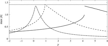
Maximum acoustic wave amplitude $|A|$ due to resonant gravity–acoustic triad interaction, as the tuning parameter ${\it\gamma}$ is varied, for three values of the parameter ${\it\alpha}$ , which controls the initial gravity-wave steepness. (——): ${\it\alpha}=1$ ; (– – –):  ${\it\alpha}=0.5$ ; (— ⋅ —): ${\it\alpha}=0.2$ . The dotted line ( $\cdots \cdots$ ) indicates the upper bound $|A|=\sqrt{2}$ implied by (6.1).

Our computations confirm that the interaction results in cyclic exchange of energy among the triad members. Figure 1 shows plots of the maximum acoustic amplitude $|A|$ reached in the course of the interaction, as ${\it\gamma}$ is varied, for three different values of ${\it\alpha}$ . For the smallest ${\it\alpha}=0.2$ , we obtain a bell-shaped curve with peak near ${\it\gamma}=0$ , similar to a classical triad where the cubic terms in (5.9) are absent (Bretherton Reference Bretherton1964). Moreover, the computed peak response is slightly less than $\sqrt{2}$ , which according to (6.1) corresponds to the perfectly tuned situation where all the energy initially in the gravity waves is transferred to the acoustic wave.

For the two larger ${\it\alpha}$ , by contrast, the response curves in figure 1 are no longer symmetric and the resonance peak is progressively shifted towards ${\it\gamma}>0$ as ${\it\alpha}$ is increased; furthermore, for the largest ${\it\alpha}=1$ , a ‘jump’ phenomenon is observed near ${\it\gamma}=4.1$ . This nonlinear-resonance behaviour is instigated by the cubic terms in (5.9), which come into play as ${\it\alpha}$ is increased and cause a shift of the gravity-wave frequency; as a result, ${\it\gamma}$ has to adjust so as to fine-tune the triad. It should be noted that the peak response remains close to the upper bound $|A|=\sqrt{2}$ irrespective of ${\it\alpha}$ , indicating that nearly all the initial gravity-wave energy can be transferred to the acoustic wave when a triad is suitably tuned.

Next, we explore the resonant excitation of acoustic waves by locally confined gravity wavepackets, based on numerical solutions of the evolution equations (5.9) and (5.10). Again, we focus on the acoustic mode $n=0$ with ${\it\kappa}=1$ and assume that no acoustic disturbance is initially present, $A(X,T=0)=0$ . Also, for simplicity as before, the two gravity-wave envelopes are taken to be equal, $S_{\pm }(X,T)\equiv S(X,T)$ , with initial condition $S(X,T=0)=S_{0}(X)$ , where $S_{0}(X)\rightarrow 0$ as $X\rightarrow \pm \infty$ . Then from (5.9) and (5.10) we deduce the conservation law

which is the wavepacket counterpart of (6.1). In all computations reported below, $S_{0}=\exp (-X^{2})$ , so the right-hand side in (6.2) equals $\sqrt{2{\rm\pi}}$ . Numerical integration of (5.9) and (5.10) was carried out using MATLAB solver ‘pdepe’.

For the assumed initial conditions, in view of (6.2),

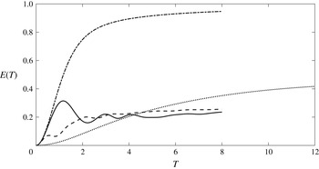
may be interpreted as the fraction of the initial gravity-wave energy transferred to the acoustic mode in the course of the nonlinear interaction. To gain some insight into this energy-transfer process, we plot in figure 2 time histories of $E(T)$ for two values of the steepness parameter ${\it\alpha}=0.2$ and $1$ . These ${\it\alpha}$ were also considered earlier in the discussion of monochromatic wavetrains, and it was found that nearly all the initial gravity-wave energy can be transferred to the acoustic wave if a triad is finely tuned (figure 1). In the case of interacting wavepackets, however, figure 2 reveals that the situation is quite different: after an initial transient growth, $E(T)$ settles to about 40 % for ${\it\alpha}=0.2$ , and to only roughly 20 % for ${\it\alpha}=1$ . Moreover, in contrast to monochromatic waves, varying ${\it\gamma}$ has no appreciable impact on the energy ultimately transferred to the acoustic wave, as illustrated in figure 2 for ${\it\gamma}=4.1$ , 0 and ${\it\alpha}=1$ . It should be noted that ${\it\gamma}=4.1$ is near while ${\it\gamma}=0$ is far away from the peak acoustic response found earlier for monochromatic waves when ${\it\alpha}=1$ (see figure 1). On the other hand, for a standard triad where the cubic terms in (5.9) are absent, $E(T)$ eventually approaches 95 % under conditions of perfect tuning ( ${\it\gamma}=0$ ).

Figure 2.

Time histories of acoustic wave energy, $E(T)$ , for certain values of the wave steepness parameter ${\it\alpha}$ and the resonance tuning parameter ${\it\gamma}$ . (——): ${\it\alpha}=1$ , ${\it\gamma}=4.1$ ;(– – –): ${\it\alpha}=1$ , ${\it\gamma}=0$ ; ( $\cdots \cdots$ ):  ${\it\alpha}=0.2$ , ${\it\gamma}=0.14$ ; (— ⋅ —): ${\it\alpha}=1$ , ${\it\gamma}=0$ and the cubic terms in (5.9) are ignored (perfectly tuned standard triad).

We conclude that, for acoustic–gravity triads involving locally confined wavepackets, the self-interaction terms in the evolution equation (5.9) seriously impede the transfer of energy to the acoustic wave. As noted earlier, these terms come into play as the steepness parameter ${\it\alpha}$ is increased and are responsible for an amplitude-dependent shift of the gravity-wave frequency. In the case of monochromatic wavetrains, it is possible to compensate for this shift by adjusting ${\it\gamma}$ , and thus obtain a tuned triad interaction that leads to the resonant behaviour displayed in figure 1. For locally confined wavepackets, however, this frequency shift creates phase differences depending on the local gravity-wave amplitude, which as time passes detune the resonant triad, inhibiting the flow of energy to the acoustic wave; the bulk of the acoustic disturbance is thus induced in the early stages of the interaction and subsequently propagates away at the group velocity of the acoustic waves. This detuning is more pronounced for larger ${\it\alpha}$ , so resonant triad interactions become a less effective coupling mechanism as the wave steepness is increased.

7. Concluding remarks

Motivated by the seminal work of Longuet-Higgins (Reference Longuet-Higgins1950), we studied resonant wave interactions of an acoustic mode with two counter-propagating subharmonic surface gravity waves in water of constant depth over a rigid bottom. It turns out that such acoustic–gravity wave triads differ fundamentally from a standard resonant triad, as the acoustic spatial scale is much longer than the gravity wavelength owing to the weak compressibility of water. Exploiting this disparity in length scales, we explained the origin of the acoustic–gravity triads suggested on numerical grounds by Kadri & Stiassnie (Reference Kadri and Stiassnie2013), and we obtained via a systematic asymptotic procedure the amplitude evolution equations governing these resonant triad interactions. The appropriate amplitude equations, apart from the expected quadratic acoustic–gravity interaction terms, also involve certain cubic gravity self-interaction terms ignored in Kadri & Stiassnie (Reference Kadri and Stiassnie2013), which arise due to the longer than usual interaction time scale. These additional terms are responsible for an amplitude-dependent shift of the gravity-wave frequency and play an important part in the energy transfer from surface to acoustic waves. Specifically, for monochromatic wavetrains, it is feasible to compensate for this shift by allowing for a detuning of the triad resonance conditions, an effect not considered in Kadri & Stiassnie (Reference Kadri and Stiassnie2013), so that still nearly all the energy initially in the gravity waves is transferred to the acoustic mode. In the more realistic scenario of locally confined wavepackets, however, the cubic self-interaction terms create phase differences depending on the local gravity-wave amplitude; this detuning effect is irreversible and seriously inhibits the flow of energy to the acoustic wave, particularly as the gravity-wave steepness is increased.

Moreover, our asymptotic analysis has brought out the key role of the parameter ${\it\alpha}$ in (4.1), which measures the gravity-wave steepness ${\it\epsilon}$ relative to the compressibility parameter ${\it\mu}$ in (2.1). According to (5.1), the peak acoustic pressure (after restoring dimensions), $p_{0}\sim 2{\it\alpha}{\it\mu}^{2}{\it\omega}|A|{\it\rho}c^{2}$ , is linearly proportional to ${\it\alpha}$ , and hence to ${\it\epsilon}$ , as well as to the local acoustic wave amplitude $|A(X,T)|$ . Thus, for given ${\it\alpha}$ , the maximum pressure amplitude $p_{max}$ is achieved for $|A|_{max}$ , the maximum value of $|A|$ realised in the course of the wave interaction. Specifically, for the scenarios considered in figure 2, when ${\it\alpha}=0.2$ (with ${\it\gamma}=0.14$ ) we find $|A|_{max}=0.96$ , whereas when ${\it\alpha}=1$ , $|A|_{max}=1.35$ and $0.36$ for ${\it\gamma}=4.1$ and $0$ , respectively. These results suggest that, although the overall energy transfer to the acoustic mode becomes less efficient as ${\it\alpha}$ is increased, the induced $p_{max}$ may still increase with the gravity-wave steepness, particularly if the frequency tuning parameter ${\it\gamma}$ is chosen appropriately.