
 LCarnot(J1B,H;oJ1B)
 E→B


1. Introduction
Generating functions play an important role in Hamiltonian mechanics and in micro-local analysis, especially in Hörmander’s calculus of Fourier integral operators [ Reference Hörmander20 ]. This construction can be seen as a particular case of more general push-forward operations in the calculus of Lagrangian submanifolds. More recently this calculus of Lagrangian submanifolds has received much attention in relation to functorial constructions of morphisms and operations in the Fukaya category [ Reference Wehrheim and Woodward53 ].
Chaperon [
Reference Chaperon9
] and Laudenbach–Sikorav [
Reference Laudenbach and Sikorav27
] used the broken geodesic approximation of the action functional in the proof of Arnold’s conjecture in the cotangent bundle. Sikorav [
Reference Sikorav44
] identified this approximation as a canonical construction of a generating function (quadratic at infinity), and also used the calculus of Lagrangian submanifolds (and the corresponding generating functions) to put the construction of [
Reference Laudenbach and Sikorav27
] in a natural setting. (See also [
Reference Chekanov10, 51
].) This technique of generating functions was then culminated by Viterbo [
Reference Viterbo48
] into a construction of some symplectic invariants. (See also [
Reference Traynor47
].) In this construction, the notions of generating functions quadratic at infinity (abbreviated as
 ${{\mathrm{GFQI}}}$
) and stable Morse theory play an important role. (See [
Reference Eliashberg and Gromov15
] for a detailed exposition on this aspect.) Kragh has been making a series of homotopical constructions to the level of a construction of Thom spectra by the technique of generating functions and applied them to the nearby Lagrangian conjecture [
Reference Kragh23, Reference Kragh24
]. (See also the joint works with others [
Reference Abouzaid, Alvarez-Gavela, Courte and Kragh1, Reference Abouzaid, Courte, Guillermou and Kragh2, Reference Abouzaid and Kragh3, Reference Abouzaid and Kragh4
].)
In [
Reference Oh33, Reference Oh34
], the first named author utilises Lagrangian intersection Floer theory to define Floer theoretic Lagrangian spectral invariants on the cotangent bundle whose coincidence with Viterbo’s
 ${{\mathrm{GFQI}}}$
spectral invariants [
Reference Viterbo48
] (up to a uniform addition by constant) is proven by Milinković [
Reference Milinković28, Reference Milinković29
]. The starting point of the construction in [
Reference Oh33
] is Weinstein’s ingenious observation [
52
], which we call Weinstein’s de-approximation, that the classical Hamilton’s action functional, denoted by
 $\mathcal A_H^{\text{cl}}$
, is a generating function of the time-one image
 $\phi_H^1(o_{T^*B})$
of the zero section of
 $T^*B$
under the Hamiltonian flow of
 $H = H(t,x)$
. (See Section 5 for the details.)
Remark 1·1 (Concerning Weinstein’s de-approximation). At this point it might be useful to set straight the history around Laudenbach–Sikorav’s finite dimensional construction and Weinstein’s infinite dimensional construction which we call ‘Weinstein’s de-approximation’. (See Section 4 for details.) When the preprint of Laudenbach–Sikorav’s paper [
Reference Laudenbach and Sikorav27
] first came out at the end of 1984, Oh was Weinstein’s graduate student. (Both Weinstein and Oh studied the preprint before its publication.) In the fall of 1987, while Oh was still a graduate student, Weinstein discovered a direct variational explanation of the essence of what Laudenbach–Sikorav did in [
Reference Laudenbach and Sikorav27
]. In one of the lectures given in his graduate course [
52
], he explained his precise formulation of the Morse family framework on the space of paths as described in the present paper. He called his variational construction the de-approximation of Laudenbach–Sikorav’s broken-trajectory approximation at that time. Then in [
Reference Oh33
], Oh utilised Weinstein’s observation as the starting point of his Floer theoretic construction of Viterbo’s generating function invariants [
Reference Viterbo48
], and called it ‘Weinstein’s de-approximation’. After that, Miliknović [
Reference Milinković28, Reference Milinković29
] employed this connection between the generating function and the action functional in his study of the equivalence between the stable Morse homology of GFQI [
Reference Traynor47, Reference Viterbo48
] and the Lagrangian intersection Floer homology [
Reference Oh33
] of the Hamiltonian isotope of the zero section of
 $T^*B$
.
The main purpose of this paper is to formulate the Legendrian counterpart thereof and provide a canonical construction of
 ${{\mathrm{GFQI}}}$
for any contact Hamiltonian isotope of the zero section of a one-jet bundle
 $J^1B$
. This is also the first step of the sequel [
Reference Oh and Yu41
] where the authors construct the Legendrian counterpart on the one-jet bundle of the first named author’s Floer theoretic construction of Lagrangian spectral invariants on the cotangent bundle. We believe that the invariants coincide with the
 ${{\mathrm{GFQI}}}$
spectral invariants constructed by Théret in [
Reference Théret46
], Bhupal [
Reference Bhupal8
] and Sandon [
Reference Sandon42
] following Viterbo’s scheme of stable Morse theory. The main step of the
 ${{\mathrm{GFQI}}}$
invariants is the existence and certain uniqueness results of the generating function quadratic at infinity which are established in [
Reference Laudenbach and Sikorav27, Reference Sikorav44
] for the existence and in [
Reference Théret46, Reference Viterbo48
] for the uniqueness. (See Section 8 for some quick review on the
 ${{\mathrm{GFQI}}}$
construction.)
The known construction of generating functions quadratic at infinity for Legendrian submanifolds in the one-jet bundle [
Reference Chaperon9, Reference Chekanov10, Reference Ferrand16
] is rather different from the natural construction of Laudenbach–Sikorav which uses a Hamiltonian variation of Bott’s finite dimensional geodesic approximation in his Morse theoretic study of the topology of loop spaces. This construction in the chain level depends on the rank N of the associated vector bundle such that the associated stable Morse homology has the limit as
 $N \to \infty$
relating to Floer homology for the action functional. (See [
Reference Milinković28, Reference Milinković29
].) This chain level study is fundamental for the aforementioned Kragh’s homotopical construction above.
It turns out that finding the contact counterpart of the aforementioned Weinstein’s de-approximation of Laudenbach–Sikorav’s construction of a ‘canonical generating function’ described in [
52
] is rather nontrivial largely because the commonly used action functional carries large degeneracy in its variational study arising from the whole set of reparametrisations of the curves. To remove this degeneracy and rigidify the relevant calculus of variations, we need to put some constraints. For this purpose, we need to do some general study of the space of (translated) horizontal paths of the contact distribution of a contact manifold
 $(M,\xi)$
and get into a little bit of Carnot-Carathéodory geometry. (See [
Reference Mitchell30
] for the relevant results and [
Reference Montgomery31
] for a nice panoramic exposition on Carnot-Carathéodory geometry.)
In the sequel [ Reference Oh and Yu41 ], utilising these background geometric preparations and analysis of (perturbed) contact instantons established in [ Reference Oh36, Reference Oh37, Reference Oh38 ], we carry out the Floer theoretic construction of Legendrian spectral invariants as mentioned above, which is the contact counterpart of the construction given in [ Reference Oh33, Reference Oh34 ].
1·1. The space of Hamiltonian-translated horizontal paths
Let
 $(M,\xi)$
be a contact manifold. A contact diffeomorphism, abbreviated as a contactomorphism,
 $\psi\;:\; M \to M$
is a diffeomorphism satisfying
 $d\psi(\xi) \subset \xi$
, and a contact vector field X is one whose flow generates an isotopy of contactomorphisms. Equivalently, X is contact if and only if the Lie derivative
 $\mathcal L_XY = [X,Y]$
is tangent to
 $\xi$
whenever the vector field Y is tangent to
 $\xi$
.
Now let
 $\xi$
be coorientable which we will assume from now on. Then we choose a contact form
 $\lambda$
, i.e., one form with
 $\xi = \ker \lambda$
. A choice of contact form induces a decomposition
 \begin{equation}TM = \xi \oplus \mathbb R \langle R_\lambda \rangle, \end{equation}
where
 $R_\lambda$
is the
 $\lambda$
-Reeb vector field uniquely determined by the equations
 \begin{align*}R_\lambda \mathbin{\lrcorner} \lambda = 1, \quad R_\lambda \mathbin{\lrcorner} d\lambda = 0.\end{align*}
The choice of contact form also enables us to associate a natural
 $\mathbb R$
-valued function given by
 $H = -\lambda(X)$
to any vector field.
Conversely, for any given
 $\mathbb R$
-valued function H, we can associate a contact vector field by the defining equation
 \begin{equation}\begin{cases}X \mathbin{\lrcorner} \lambda = -H \\X \mathbin{\lrcorner} d\lambda = dH - R_\lambda[H]\lambda.\end{cases}\end{equation}
(See [
Reference Geiges17
, theorem 2·3] for the proof, for example, but with different sign convention of
 $H\;:\!=\; \lambda(X)$
. In this paper, we systematically follow the sign convention of [
Reference Bravetti, Cruz and Tapias7, Reference de León and Lainz Valcázar13, Reference Oh36
] in our sometimes rather elaborate calculations. We refer the reader to Section 2 for a summary of contact Hamiltonian calculus in our convention. To avoid confusion arising from this difference of conventions from other literature, we make our contact Hamiltonian calculus self-contained.)
The contact Hamilton’s equation
 $\dot y = X_H(t,y)$
can be rewritten as
 \begin{equation}\begin{cases}(\dot \gamma - X_H(t,\gamma(t)))^\pi = 0 \\\gamma^*\lambda + H(t,\gamma(t))dt = 0\end{cases}\end{equation}
by splitting the equation into the contact distribution direction and the Reeb direction. This decomposition suits well with the analytic study of perturbed contact instanton equation as presented in [ Reference Oh36, Reference Oh37 ]. A particular type of perturbed action functional is introduced by the first-named author in [ Reference Oh36, Reference Oh37 ] for the variational study of this equation under the general Legendrian boundary condition in any contact manifold.
Remark 1·2. We would like to emphasise that readers should take our sign convention [ Reference Bravetti, Cruz and Tapias7, Reference de León and Lainz Valcázar13, Reference Oh36 ] (or others, if any) as a whole package which should be consistently used in the various calculations we involve for the purpose of this paper.
By definition of (coorientation-preserving) contactomorphism
 $\psi$
of a coorientable contact structure
 $\xi$
equipped with a contact form
 $\lambda$
, we can write
 $\psi^*\lambda = f \lambda$
for some positive function
 $f = f_\psi^\lambda$
. Writing
 $g = g_\psi^\lambda \;:\!=\; \log f$
, which we call the conformal exponent of contactomorphism
 $\psi$
, we have
 \begin{align*}\psi^*\lambda = e^{g_\psi} \lambda.\end{align*}
Notation 1·3. Let
 $H = H(t,y)$
be a contact Hamiltonian. We denote by
 $\psi_H^t$
the contact Hamiltonian flow of H. We denote by
 $\phi_H^t$
the isotopy defined by
 \begin{equation}\phi_H^t\;:\!=\; \psi_H^t (\psi_H^1)^{-1}.\end{equation}
We remark that
 $\phi_H^1 = {{\mathrm{Id}}}$
and
 $\phi_H^0 = (\psi_H^1)^{-1}$
. The curve
 $\gamma$
defined by
 $\gamma(t) \;:\!=\; \phi_H^t(y)$
solves the final-value problem
 \begin{align*}\dot \gamma = X_H(\gamma), \quad \gamma(1) = y\end{align*}
for the given point y. (See [ Reference Oh34 ] for a systematic discussion on this point of view.)
Definition 1·4 (Perturbed action functional). Let
 $H = H(t,y)$
be a contact Hamiltonian and denote by
 $\mathcal L(M)$
the free path space, i.e., the set of smooth maps
 $\gamma\;:\; [0,1] \to M$
. We define the functional
 $\mathcal A_{H;\lambda}\;:\; \mathcal L(M) \rightarrow \mathbb R$
by
 \begin{eqnarray}\mathcal A_{H;\lambda}(\gamma) = \int_0^1 e^{g_{(\phi_H^t)^{-1}} (\gamma(t))}\left(\lambda(\dot \gamma (t)) + H_t (\gamma (t))\right) \, dt.\end{eqnarray}
Note that, when
 $H = 0$
, we have
 \begin{align*}\mathcal A_{0;\lambda} (\gamma)\;:\!=\; \int_0^1 \gamma^* \lambda\end{align*}
which is the standard contact action functional for the Reeb flow. Since we will not vary
 $\lambda$
, we will simply omit the dependence of
 $\lambda$
and write
 $\mathcal A_H$
and
 $\mathcal A_0$
respectively.
Remark 1·5.
-
(1) Under the assignment
the map \begin{align*}\Phi_H(\gamma)(t) = (\phi_H^t)^{-1}(\gamma(t)) = \overline\gamma(t),\end{align*}
$\Phi_H$
transforms paths with Legendrian boundary condition from
$(R_0,R_1)$
to
$(\psi_H(R_0),R_1)$
of
$\gamma$
at
$t = 0, \, 1$
for a given pair of Legendrian submanifolds
$(R_0,R_1)$
. (See (2·11) for the precise definition.)
-
(2) In fact, one can associate an action functional to each time-dependent family of contact forms
$\{\lambda^s\}_{s \in [0,1]}$
by which we will again simply write as
\begin{align*}\mathcal A_{\{\lambda^{(\cdot)}\}}(\gamma)\;:\!=\; \int_0^1 \lambda^t(\dot \gamma(t))dt\end{align*}
$\mathcal A_0$
for the simplicity of notation. The action functional
$\mathcal A_H$
is obtained by considering the family given by See Lemma 2·8.
\begin{align*}\lambda^s = ((\phi_H^s)^{-1})^*\lambda = (\phi_H^s)_*\lambda.\end{align*}


We attract the reader’s attention to the fact that the value of
 $\mathcal A_H$
at any Hamiltonian trajectory is automatically zero which exhibits the nature of constrained variation with the contact Hamiltonian trajectories in the point of view of the calculus of variation. (See the discussion of Section 3, especially Theorem 3·2, for further elaboration.) This has led us to consider the restriction of
 $\mathcal A_H$
to the following Carnot-type path space.
Definition 1·6 (Translated horizontal paths). For each given Hamiltonian
 $H = H(t,y)$
, we define the subset
 \begin{align*}\mathcal L^{\text {Carnot}}(M,H) \subset \mathcal L(M)\end{align*}
to be the set of piecewise smooth continuous curves
 $\gamma\;:\;[0,1] \to M$
that satisfy
 \begin{equation}\gamma^*\lambda + H(t,\gamma(t)) \, dt = 0.\end{equation}
We call an element
 $\gamma$
therein an H-translated horizontal path of the contact distribution
 $\xi$
, and the set of such paths the H-Carnot path space.
Remark 1·7. Recall that in thermodynamics the notion of a Carnot path is a finite succession of paths which are alternately adiabatic and isothermal. Such a path belongs to the realm of piecewise smooth horizontal paths for the thermodynamic contact form, e.g.,
 $\lambda = dU - TdS + PdV$
in
 $J^1\mathbb R^2 \cong \mathbb R^5$
. This is the reason for our naming of (Hamiltonian-translated) Carnot path space here.
In fact, if we define
 $\overline \gamma(t)\;:\!=\; (\phi_H^t)^{-1}(\gamma(t))$
, (1·6) is equivalent to saying that
 $\overline \gamma$
is tangent to the contact distribution, i.e., that it satisfies
 \begin{equation}\frac{d \overline \gamma}{dt}\in \xi.\end{equation}
In Carnot-Carathéodory geometry, such a path
 $\overline \gamma$
is called a horizontal curve of the distribution
 $\xi$
. Since the contact distribution satisfies the Hörmander’s condition [
Reference Hörmander19
], it is an immediate consequence of the general result by Chow [
Reference Chow11
] that
 $\mathcal L^{\text {Carnot}}(M,H)$
is locally transitive in the sense that any point
 $p\in M$
can be joined to a given point
 $m \in M$
, provided p is sufficiently close to m. (See [
Reference Mitchell30
] for a quick summary of the Carnot-Carathéodory geometry needed for our discussion. For the reader’s convenience, we provide some quick discussion on the Carnot-Carathéodory metrics on M equipped with a distribution that satisfies Hörmander’s condition [
Reference Hörmander19
] and its relationship with the above translated Carnot paths in Appendix A.)
However, a priori it is not clear whether this subset carries a smooth structure in the sense of an infinite dimensional Fréchet manifold on which we can do calculus of variation. In this regard, we prove the following.
Theorem 1·8. For any smooth Hamiltonian
 $H =H(t,y)$
, the subset
 \begin{align*}\mathcal L^{\text {Carnot}}(M,H) \subset \mathcal L(M)\end{align*}
is a smooth submanifold of the free path space
 $\mathcal L(M)$
and so carries the induced Fréchet manifold structure.
We would like to highlight that this smooth Fréchet manifold structure does not involve any type of transversality or nondegeneracy hypothesis on the Hamiltonian H but holds for any smooth Hamiltonian. We alert readers that when
 $H = 0$
this is nothing but the set of horizontal curves of the contact distribution
 $\xi$
.
Corollary 1·9. The set of piecewise smooth horizontal paths of the contact distribution of
 $(M,\xi)$
is a Fréchet manifold.
1·2. Morse family and generation of Legendrian submanifolds
To facilitate our discussion, especially when we deal with the infinite dimensional case of the action functional, we start by considering the following general notion of Morse family in the theory of generating functions. (See [ Reference Lees25, 49 ] for the earlier usage of generating functions defined on the general fiber bundles and [ Reference Castrillón and Ratiu12 , section 3, definition 1] for the explicitly written definition of the term Morse family in the sense of Definition 1·13 below for the finite dimensional case, and see [ Reference Do and Oh14 ] for the treatment of the infinite dimensional case.)
Remark 1·10. See Section 8 for the definition and properties of generating functions. Mostly in the literature, especially in relation to the study of symplectic topology of cotangent bundles (resp. to that of contact topology of one-jet bundles), generating functions defined on a vector bundle are considered [ Reference Bhupal8, Reference Laudenbach and Sikorav27, Reference Sandon42, Reference Sikorav44, Reference Théret46, Reference Traynor47, Reference Viterbo48 ]. However one can consider a general Morse family to construct a priori a more general class of exact Lagrangian (resp. Legendrian) submanifolds than the Hamiltonian isotopes as shown in [ Reference Castrillón and Ratiu12, Reference Do and Oh14, Reference Lees25, 49 ]. It is an interesting open problem to see whether this family of exact Lagrangian submanifolds would contain a counter-example of the nearby Lagrangian conjecture by developing a more functorial study of the construction utilising some ‘additive structures’ of the Morse family and of the family of associated Lagrangian submanifolds [ Reference Hörmander20, Reference Viterbo48 ].
Let
 $\pi\;:\;\mathcal E \to B$
be a fiber bundle, where B is finite dimensional but
 $\mathcal E$
is not necessarily so. We choose a suitable Ehresmann connection
 $\Gamma$
for
 $\pi$
, i.e., a splitting
 \begin{equation}\Gamma\;:\; \quad T\mathcal E = VT\mathcal E \oplus HT\mathcal E,\end{equation}
where
 $VT_e\mathcal E\;:\!=\; (d_e\pi)^{-1}(0)$
is a vertical tangent space at e, and
 $HT_e\mathcal E$
is a horizontal one. The derivative
 $d\pi$
restricts to an isomorphism
 \begin{equation}d\pi_e\;:\; HT_e \mathcal E \to T_{\pi(e)} B\end{equation}
at all
 $e \in E$
. When we are given a smooth function
 $S\;:\;\mathcal E \to \mathbb R$
, we consider the diagram

and decompose its differential
 $dS = d^vS + D^hS$
, where we define
 \begin{align*}d^v S(e) = dS(e)|_{VT_e\mathcal E}, \quad D^hS(e) = dS(e)|_{HT_e \mathcal E},\end{align*}
where the notation indicates the vertical derivative
 $d^vS$
does not depend on the connection
 $\Gamma$
while
 $D^hS$
does. (See (8·2) for precise description of
 $d^vS$
as the fiber derivative which is defined canonically.)
Remark 1·11. At the moment, we avoid attempting to provide precise meaning of the dual space of an infinite dimensional space (e.g., in the definition of ‘cotangent bundle’) which will inevitably involve nontrivial functional analytical issues. (See [
Reference Kriegl and Michor22
] for an excellent exposition on such matters.) Therefore readers had better take the current discussion in the formal level (as in the variational calculus) to motivate further discussion below. For the readers who feel uneasy of the formal discussion, we refer them to [
Reference Do and Oh14
, appendix B] for some detailed rigorous discussion on this dimension counting in the infinite dimensional fibration
 $\mathcal E \to B$
.
We define
 \begin{align*}\Sigma_{S}\;:\!=\; (d^vS)^{-1}(o_{(VT)^*\mathcal E}) = \{ e \in \mathcal E \mid d^vS(e) = 0\},\end{align*}
where
 $o_{ (VT)^*\mathcal E}$
is the zero section of the bundle
 $(VT)^*\mathcal E \to \mathcal E$
dual to
 $VT\mathcal E \to \mathcal E$
. We then define a map
 $\iota_S\;:\; \Sigma_{S} \to J^1B$
by
 \begin{eqnarray}\iota_{S}(e) &\;:\!=\; & \left(\pi(e), D^hS(e) \circ (d\pi_e|_{HT_e\mathcal E })^{-1}, S(e)\right) \end{eqnarray}
 \begin{eqnarray}& = & \left(\pi(e), dS(e) \circ (d\pi_e|_{T_e \mathcal E})^{-1}, S(e)\right)\!,\end{eqnarray}
where the latter identity follows since
 $e \in \Sigma_S$
. It shows that the definition of the map
 $\iota_S$
involves an Ehresmann connection but its image does not depend on the choice of an Ehresmann connection.
Remark 1·12.
-
(1) We remark that the image of
$\iota_S$
could a priori be a pathological space by two reasons: Firstly
$\Sigma_{S}$
can be a pathological space unless S satisfies suitable transversality hypothesis. Secondly even if
$\Sigma_S$
carries a smooth structure, the map
$\iota_S$
can be singular. However both maps,
$d^vS\;:\; E \to E^*$
and
$\iota_S\;:\; \Sigma_S = (d^vS)^{-1}(0) \subset E \to J^1B$
, are defined one after the other for any differentiable function S without any kind of transversality condition. We denote by
$R_S$
the image,
$\iota_S(\Sigma_S) \subset J^1B$
. -
(2) Under the transversality hypothesis (1·13) below,
$R_S$
becomes the (smooth) push-forward of the Legendrian graph under the projection
\begin{align*}\text{Image} \, j^1S \subset J^1\mathcal E\end{align*}
$\pi_\mathcal E\;:\; \mathcal E \to B$
in the calculus of Legendrian submanifolds.
-
(3) We recall that under the same transversality hypothesis on S, the map
$i_S\;:\; \Sigma_S \to T^*B$
given by defines a Lagrangian immersion which is the push-forward of
\begin{align*}i_S(e)\;:\!=\; (D^hS(e) \circ (d\pi_e|_{HT_e\mathcal E})^{-1})\end{align*}
$\operatorname{Graph} dS \subset T^*\mathcal E$
under the same projection
$\pi_\mathcal E\;:\; \mathcal E \to B$
in calculus of Lagrangian submanifolds [
51, Reference Wehrheim and Woodward53
]. The above construction is nothing but the contact analogue of this operation. (We refer to [
Reference Oh and Park40
] for the details on the Legendrian correspondence.)


We now consider the following standard transversality hypothesis
 \begin{equation}d^v S \pitchfork o_{ (VT)^*\mathcal E}.\end{equation}
This ensures smoothness of
 $\Sigma_S$
.
Definition 1·13 (Morse family). Consider a smooth fibration
 $\pi\;:\; \mathcal E \to B$
and a smooth function
 $S \;:\; \mathcal E \to \mathbb R$
visualised in the diagram (1·10). We say S is
 $\pi$
-relative Morse with respect to the fibration
 $\pi\;:\; \mathcal E \to B$
, if it satisfies (1·13), or simply a Morse family when explicit mentioning with respect to the fibration is not needed.
A basic result is that the map
 $\iota_S \;:\; \Sigma_S \to J^1B$
given in (1·11) defines a Legendrian immersion for any Morse family
 $S\;:\; \mathcal E \to \mathbb R$
. (See [
Reference Hörmander20, Reference Lees25, 49
] in the symplectic/Lagrangian context which automatically imply the contact/Legendrian context, and [
Reference Do and Oh14
, appendix B] for detailed explanation in the infinite dimensional setting.)
Definition 1·14. Let
 $\mathcal E \to B$
be a fiber bundle and
 $S\;:\; \mathcal E \to \mathbb R$
be a Morse family. We say S generates a Lagrangian submanifold
 $L \subset T^*B$
(resp. a Legendrian submanifold
 $R \subset J^1B$
), if L (resp. R) is the image of a Lagrangian immersion
 $i_S\;:\; \Sigma_S \to T^*B$
(resp. a Legendrian immersion
 $\iota_S\;:\; \Sigma_S \to J^1B)$
defined above, and call S a generating function of L (resp. of R).
We denote by
 \begin{align*}\mathfrak{Leg}(J^1B) \, \text{(resp. $\mathfrak{Leg}_0(J^1B)$)}\end{align*}
the set of Legendrian submanifolds of
 $J^1B$
(resp. those Legendrian isotopic to the zero section
 $R_0 = o_{J^1B}$
).
1·3. Action functional as a canonical generating function on
$J^1B$

Now we restrict contact manifolds to the case of one jet bundles
 $J^1B$
of a smooth manifold B equipped with the standard contact structure
 $\xi =\ker \lambda$
given by the standard contact form
 $\lambda = dz - pdq$
. We then consider the class of Legendrian submanifolds given by the Hamiltonian isotope
 $R = \psi_H^1(o_{J^1B})$
of the contact Hamiltonian
 $H = H(t,y)$
with
 $y = (x,z) \in J^1B$
. We denote by
 \begin{equation}\pi_B\;:\; J^1B \to B,\quad \pi_{T^*B}\;:\; J^1B \to T^*B, \quad z\;:\; J^1B \to \mathbb R\end{equation}
the obvious projections. Then we can write
 \begin{align*}\lambda = dz - \pi^*\theta, \quad \pi = \pi_{T^*B},\end{align*}
where
 $\theta = pdq$
is the Liouville one-form on the cotangent bundle
 $T^*B$
.
We also specialise the action functional (1·5) to the case of
 $J^1B$
. As mentioned above the value of
 $\mathcal A_H$
at any Hamiltonian trajectory vanishes. Largely because of this, finding a right formulation of the contact counterpart of Weinstein’s de-approximation [
52
], more precisely a canonical variational construction of a generating function from Hamilton’s action functional, is much more nontrivial than expected, whose explanation is now in order. First of all, we need to consider the following variation of
 $\mathcal A_H$
, which we call the effective action functional, on the aforementioned Carnot-type path space.
Definition 1·15 (Effective action functional). We define
 $\widetilde{\mathcal{A}}_H\;:\; \mathcal L(J^1B)\to \mathbb R$
to be
 \begin{eqnarray}\widetilde{\mathcal{A}}_H(\gamma) & = & - \mathcal A_H (\gamma) + z(\gamma(1)) \\[5pt]& = & - \int_0^1 e^{g_{(\phi_H^t)^{-1}} (\gamma (t))} (\lambda_{\gamma(t)} (\dot \gamma (t)) + H(\gamma(t))) dt + z(\gamma(1)).\end{eqnarray}
We mention that if
 $\gamma$
is a Hamiltonian trajectory, the action is reduced to
 \begin{align*}\widetilde{\mathcal{A}}_H(\gamma) = z(\gamma(1)).\end{align*}
(We refer to Section 5, especially Remark 5·2, for the explanation on our adoption of the sign used here and for further expounding of the definition of
 $\widetilde{\mathcal{A}}_H$
.)
Then we denote by
 \begin{align*}\mathcal A _H^{CC} \;:\; \mathcal L ^{\text {Carnot}} (J^1B,H) \to \mathbb R\end{align*}
the restriction of
 $\widetilde{\mathcal{A}} _H$
to
 $\mathcal L ^{\text {Carnot}} (J^1B,H)$
and also call it (restricted) effective action functional. (Here ‘CC’ stands for Carnot and Carathéodory.)
Then we consider the subset
 \begin{align*}\mathcal L^{\text {Carnot}}_{0}(J^1B,H;\;o_{J^1B}) \subset \mathcal L^{\text {Carnot}}(J^1B,H)\end{align*}
consisting of the paths
 $\gamma \in \mathcal L^{\text {Carnot}}(J^1B,H)$
satisfying
 $\gamma(0) \in o_{J^1B}$
in addition. Finally we consider the fibration
 \begin{align*}\Pi\;:\; \mathcal L_{0}^{\text {Carnot}}(J^1B, H;\;o_{J^1B}) \to B\end{align*}
with
 $\Pi = \pi_B \circ \operatorname{ev}_{1}$
for the evaluation map
 $\operatorname{ev}_{1}$
given by
 $\operatorname{ev}_{1}(\gamma) = \gamma(1)$
.
The following theorem is the contact counterpart of Weinstein’s variational construction of a generating function from Hamilton’s action functional in symplectic geometry. It also proves that the functional
 $\mathcal A _H^{CC} \;:\; \mathcal L ^{\text {Carnot}} (J^1B,H;\;o_{J^1B}) \to \mathbb R$
is a Morse family for any Hamiltonian H.
Theorem 1·16. Consider the space
 $\mathcal L_{0}^{\text {Carnot}}(J^1B, H;\;o_{J^1B})$
and the diagram

for any H. Then the following holds:
-
(i) the functional
$\mathcal A_H^{CC} \;:\; \mathcal L ^{\text {Carnot}} (J^1B,H;\;o_{J^1B}) \to \mathbb R$
satisfies (1·13) with S replaced by
$\mathcal A_H^{CC}$
; -
(ii) it generates
$R = \psi_H^1(o_{J^1B})$
with respect to the fibration
\begin{align*}\Pi\;:\; \mathcal L_{0}^{\text {Carnot}}(J^1B, H;\;o_{J^1B}) \to B.\end{align*}


1·4. Broken trajectory approximations and contact Hamiltonian calculus
After we identify the correct action functional generating the given contact Hamiltonian isotope of the Legendrian submanifold
 $o_{J^1B}$
, we now apply the broken trajectory approximation to give a ‘canonical’ construction of a
 ${{\mathrm{GFQI}}}$
of any Hamiltonian isotope of the zero section in the one-jet bundle. Motivated by Theorem 1·16 and Chaperon [
Reference Chaperon9
], Laudenbach–Sikorav’s construction [
Reference Laudenbach and Sikorav27
] in the symplectic case, we perform the contact counterpart of Laudenbach–Sikorav’s broken trajectory approximation for the effective action functional
 $\mathcal A_H^{\text{CC}}$
.
We start by briefly recalling the construction given in [
Reference Chaperon9, Reference Laudenbach and Sikorav27
]. To avoid notational complications, we consider the case of
 $T^*T^n$
as in [
Reference Chaperon9
] and utilise the ‘linear’ structure of
 $T^n$
in the following summary. We take a partition
 \begin{align*}0 = t_0 \lt t_1 \lt \cdots \lt t_N = 1, \quad t_i = \frac{i}{N}\end{align*}
and consider the set of piecewise smooth paths
 $\ell\;:\;[0,1] \to T^*T^n$
with jump at each
 $t_i$
satisfying the initial condition
 $\ell(0) \in o_{T^*T^n}$
, smooth on each semi-open interval
 $[t_i,t_{i+1})$
for
 $i =0, \cdots N-1$
and having the left limit

. We denote

Denote
 $(X_i,P_i) = (q_i^+, p_i^+) - (q_i^-, p_i^-)$
and regard
 $(X,P) = \prod_{i=1}^{N-1} (X_i,P_i)$
as an element of
 $T^n \times (T^*T^n)^{N-1}$
whose dimension is given by
 $n + 2(N-1) n \lt \infty$
. To get rid of the additional freedom, we specify the path segment
 $\ell_{[t_i,t_{i+1}]}$
to be
 \begin{equation}\ell_i(t) = \phi_H^t(q_i^+,p_i^+), \quad t \in [t_i, t_{i+1}].\end{equation}
Then we denote by
 $\ell_{(X,P)}$
the corresponding piecewise smooth paths. We denote the corresponding set of piecewise smooth paths with jumps by
 $E_N$
, define the projection map
 $\pi_N\;:\; E_N \to T^n$
to be
 \begin{align*}\pi_N(X,P) = \pi_{T^*T^n}(q_N^-, p_N^-) = \pi_{T^*T^n}\left(\ell_{(X,P)}(1)\right)\end{align*}
and the function
 $S_N\;:\; E_N \to \mathbb R$
by
 \begin{equation}S_N(X,P) \;:\!=\; \mathcal A^{\text{cl}}_H(\ell_{(X,P)}),\end{equation}
where
 $\mathcal A^{\text{cl}}_H$
is Hamilton’s action functional given by
 \begin{align*}\mathcal A^{\text{cl}}_H(\zeta) = \int \zeta^*\theta - H(t,\zeta(t))dt\end{align*}
for a path
 $\zeta\;:\;[0,1] \to T^*T^n$
with the Liouville one-form
 $\theta = p\, dq$
on
 $T^*T^n$
. In this way, we have a diagram (1·10) for each given N. These being said the main result of [
Reference Chaperon9, Reference Laudenbach and Sikorav27
] is that this diagram generates the Lagrangian submanifold
 $\phi_H^1(o_{T^*T^n})$
for all sufficiently large N.
The following point is the main difference of our construction from that of [
Reference Chaperon9, Reference Laudenbach and Sikorav27
] in addition to our usage of rather peculiar type of contact action functional
 $\mathcal A_H^{\text{CC}}$
to handle the large degeneracy of the more standard action functional.
Consequently: One crucial deviation of our broken trajectory approximation from that of [
Reference Chaperon9, Reference Laudenbach and Sikorav27
] is that in the current contact case, we also need to insert some additional horizontal trajectories in between every consecutive pair of contact Hamiltonian trajectories by bisecting each interval
 $[t_i,t_{i+1}]$
for
 $i =1, \ldots, N-1$
. (We refer to Section 9 for the details. See Figure 1 for its visualisation.)
A broken trajectory in
 $J^1B$
. Each arc
 $\gamma_k$
corresponds to a piece of contact Hamiltonian flow from
 $y_{k-1}^+$
to
 $y_k^-$
, and each
 $\mu_k$
is the horizontal lift of a geodesic flow, ending at
 $y_k^+$
. The dotted lines indicate jumps in the p-coordinate between
 $\gamma_k$
and
 $\mu_k$
. The trajectory starts at
 $y_0 = (q_0,0,0)$
and ends at
 $y_N^-=(q_N^-,p_N^-,z_N^-)$
.

So the relevant broken trajectories are the consecutive unions of the concatenated pairs of contact Hamiltonian trajectories and horizontal paths. This whole process is canonical modulo the degrees of freedom, again given by
 \begin{align*}\dim T^n + 2(N-1) \dim T^n = n+2(N-1)n.\end{align*}
We summarise our construction into the following theorem somewhat vaguely here, but the full explanations and details of the algorithm appear in Sections 9–12 and its proof in Section 13.
Theorem 1·17. Let B be any compact manifold. Then there is a ‘canonical’ algorithm of a finite dimensional Morse family (1·10) with
 $\mathcal E = E^N$
,
 $S = S_N$
and
 $\pi = \pi_N$
which ‘approximates’ the effective action functional
 $\mathcal A_H^{\text CC}$
that gives rise to a
 ${{\mathrm{GFQI}}}$
of any contact Hamiltonian isotope of the zero section
 $o_{J^1B}$
.
Largely due to the nontrivial presence of conformal exponent of the contactomorphism unlike the symplectomorphism, the relevant contact Hamiltonian calculus is significantly more difficult than the symplectic one. We would like to recommend readers to compare the degree of complexity of the calculations performed here and those in [ Reference Laudenbach and Sikorav27 ]. It makes the computations entering in the critical point analysis of the action functional or its broken trajectory approximations much harder than the symplectic case of [ Reference Chaperon9, Reference Laudenbach and Sikorav27 ]. Unlike the symplectic case, it also requires us to perform very careful and precise tensorial calculations based on the systematic contact Hamiltonian calculus. Such a systematic calculus has been developed and used by the first named author in relation to the series of works on contact instantons starting from [ Reference Oh36 ]. (This calculus is a continuation of those adopted in [ Reference Bravetti, Cruz and Tapias7 ] with all the sign conventions both in symplectic and contact Hamiltonian calculi which are also compatible with those listed in List of conventions of [ Reference Oh35 ] in the symplectic case.)
The organization of the paper is now in order. In Section 2, we collect some useful results concerning the contact Hamiltonian dynamics which will enable us to systematically study the calculus of variations of the perturbed action functional
 $\mathcal A_H$
. We mostly follow the exposition of [
Reference Bravetti, Cruz and Tapias7
] on contact Hamiltonian mechanics, and [
Reference Oh36
] for a more extensive systematic exposition on contact Hamiltonian calculus. In Section 3, we give the proof of Theorem 1·8. After these preliminaries on general contact Hamiltonian geometry are given, the paper is divided into two parts. Part I contains the formulation of the contact analogue of Weinstein’s de-approximation, and the proof of Theorem 1·16. Part II then contains the aforementioned broken trajectory approximation of the effective action functional
 $\mathcal A_H^{\text{CC}}$
as a canonical construction of a
 ${{\mathrm{GFQI}}}$
for any Hamiltonian isotope of the zero section in the one-jet bundle. Finally we collect some background material in Appendix A and technical calculations in Appendix B and C which are postponed from the main text of the paper.
Conventions and notations.
-
(1) (Contact Hamiltonian) The contact Hamiltonian of a time-dependent contact vector field
$X_t$
is given by We denote by
\begin{align*}H\;:\!=\; - \lambda(X_t).\end{align*}
$X_H$
the contact vector field whose associated contact Hamiltonian is given by
$H = H(t,y)$
, and its flow by
$ \psi^t_H $
.
-
(2) When
$\psi = \psi^1_H$
, we say H generates
$\psi$
and write
$H \mapsto \psi$
. -
(3) We use the notation
$\phi_H^t\;:\!=\; \psi_H^t (\psi_H^1)^{-1}$
. (We warn readers that we also use the same notation
$\phi_H^t$
for the symplectic Hamiltonian flow to be consistent with the notation used in [
Reference Oh33, Reference Oh34
]. The meaning thereof should be clear from the context, hopefully.) -
(4) We will try to consistently use the following notations whenever appropriate:
-
(i) (q, p, z) a point of
$J^1B$
or the canonical coordinates thereof; -
(ii)
$x = (q,p)$
a point of
$T^*B$
; -
(iii)
$y = (x,z)$
a point in
$J^1B$
; -
(iv) e or (q, e) a point in a vector bundle
$E \to B$
with
$q = \pi_E(e)$
.
-
-
(5) (Reeb vector field) We denote by
$R_\lambda$
the Reeb vector field for the contact form
$\lambda$
and its flow by
$\phi^t_{R_\lambda}$
. -
(6) R: a Legendrian submanifold.
-
(7)
$\mathcal L _0 (J^1B;\; R)$
: The space of paths
$\gamma$
with
$\gamma(0) \in R$
. -
(8)
$ \mathcal L^\pi_0 (J^1B;\; R)$
: The space of horizontal paths
$\gamma$
with
$\gamma(0) \in R$
. -
(9)
$\mathcal L^{\text{ Carnot}}_0 (J^1B,H;\; R)$
: The space of H-Carnot paths (or simply Carnot paths)
$\gamma$
with
$\gamma(0) \in R$
.





2. Preliminaries
Let
 $(M,\xi)$
be a cooriented contact manifold and let
 $\lambda$
be a contact form with
 $\xi = \ker \lambda$
. Denote by
 ${\operatorname{Cont}}(M,\xi)$
(resp.
 ${\operatorname{Cont}}_0(M,\xi)$
) the set of contact diffeomorphisms (resp. the identity component thereof).
Definition 2·1. For a given coorientation preserving contact diffeomorphism
 $\psi$
of
 $(M,\xi)$
we call the function g appearing in
 \begin{align*}\psi^*\lambda = e^g \lambda\end{align*}
the conformal exponent for
 $\psi$
and denote it by
 $g = g_\psi$
.
Definition 2·2. A vector field X on
 $(M,\xi)$
is called contact if there exists a smooth function
 $f\;:\; M \to \mathbb R$
such that
 \begin{align*}\mathcal L_X \lambda = f \lambda.\end{align*}
The associated function H defined by
 \begin{equation}H = - \lambda(X)\end{equation}
is called the contact Hamiltonian of X. We also call X the contact Hamiltonian vector field associated to H.
A straightforward calculation shows
 \begin{align*}f = - R_\lambda[H].\end{align*}
Here we denote by
 $R_\lambda$
the Reeb vector field of
 $\lambda$
, i.e., the unique vector field X satisfying
 $X \rfloor d\lambda = 0, \, X\rfloor \lambda = 1$
. It is nothing but the Hamiltonian vector field associated to the constant function
 $H \equiv -1$
.
The following systematic notation will be useful to designate the Hamiltonian to a given contact isotopy as in symplectic topology [ Reference Oh and Müller39 ]. As practiced in the first-named author’s articles [ Reference Oh36, Reference Oh37 ], we adopt the following definition.
Definition 2·3 (Developing map). Let
 $\lambda$
be a contact form of
 $(M,\xi)$
. We define
 \begin{equation}{\operatorname{Dev}}_\lambda\;:\; \mathcal P({\operatorname{Cont}}(M,\xi)) \to C^\infty([0,T] \times M,\mathbb R)\end{equation}
by assigning its
 $\lambda$
-contact Hamiltonian functions
 \begin{equation}{\operatorname{Dev}}_\lambda(\ell)(t,x)\;:\!=\; -\lambda\left(\frac{\partial \ell}{\partial t}(t,\ell_t^{-1}(x))\right)\!.\end{equation}
Unravelling this definition, we have
 ${\operatorname{Dev}}_\lambda(\ell)(t,x) = H(t,x)$
if
 $X_t$
is the contact vector field as in Definition 2·2. We denote by
 $X \mapsto \psi$
if
 $\psi = \psi_H^1$
.
For a given general function H, the associated contact Hamiltonian vector field
 $X_H$
has decomposition
 \begin{align*}X_H = X_H^\pi - H R_\lambda \in \xi \oplus \mathbb R \langle R_\lambda \rangle\end{align*}
from (1·2) where the projection
 $X_H^\pi$
to
 $\xi$
is uniquely determined by the equation
 \begin{align*}X_H^\pi \rfloor d\lambda = dH - R_\lambda[H] \lambda\end{align*}
or equivalently
 \begin{equation}dH = X_H \rfloor d\lambda + R_\lambda[H] \lambda.\end{equation}
Example 2·4. Let
 $H\;:\;\mathbb R^{2n+1} \to \mathbb R$
be a smooth function on
 $\mathbb R^{2n+1} = J^1\mathbb R^n$
(or in Darboux coordinates). Then the contact Hamiltonian vector field
 $X_H$
is given by
 \begin{eqnarray}X_H & =& X_H^\pi -H R_\lambda =\sum_{i=1}^n \left(\frac{\partial H}{\partial p_i} \frac{D}{\partial q_i} - \frac{D H}{\partial q_i} \frac{\partial}{\partial p_i}\right)- H \frac{\partial}{\partial z} \\[5pt] & = & \sum_{i=1}^n \frac{\partial H}{\partial p_i} \frac{\partial}{\partial q_i} -\left(\frac{\partial H}{\partial q_i} + p_i \frac{\partial H}{\partial z}\right)\frac{\partial}{\partial p_i}+ \left(\left\langle p, \frac{\partial H}{\partial p}\right \rangle - H\right)\frac{\partial}{\partial z}, \end{eqnarray}
where the set
 $\left\{ {D}/{\partial q_i}, {\partial}/{\partial p_i}, {\partial}/{\partial z} \right\}$
with
 ${D}/{\partial q_i} \;:\!=\; {\partial}/{\partial q_i} + p_i({\partial}/{\partial z})$
is the associated Darboux frame, i.e., a frame of TM which satisfies
 \begin{align*}R_\lambda = \frac{\partial}{\partial z}, \quad \xi = \operatorname{span} \left\{ \frac{D}{\partial q_i}, \frac{\partial}{\partial p_i}\right\},\end{align*}
and
 $d\lambda({D}/{\partial q_i},{\partial}/{\partial p_i}) = \delta_{ij}$
for
 $1 \leq i, \, j \leq n$
. Therefore the associated contact Hamilton’s equation is given by
 \begin{equation}\begin{cases}\dot q_i = \dfrac{\partial H}{\partial p_i}, \\[9pt] \dot p_i = -\dfrac{D H}{\partial q_i} \left(= -\dfrac{\partial H}{\partial q_i} - p_i \dfrac{\partial H}{\partial z}\right)\!, \\[9pt] \dot z = \left\langle p, \dfrac{\partial H}{\partial p}\right \rangle - H. \end{cases}\end{equation}
Lemma 2·5. Solving contact Hamilton’s equation
 $\dot y = X_H(t,y)$
is equivalent to finding
 $\gamma:\mathbb R \to M$
that satisfies
 \begin{equation}(\dot \gamma - X_H(t,\gamma(t)))^\pi = 0, \quad \gamma^*\lambda + H(t,\gamma(t))dt = 0.\end{equation}
For the later purpose, we introduce the following proposition providing an explicit relationship between the contact Hamiltonians and the conformal exponents of a given contact isotopy.
Proposition 2·6 ([
Reference Oh36
, proposition 2·17]). Let
 $\Psi = \{\psi_t\}$
be a contact isotopy of
 $(M, \xi = \ker \lambda)$
with
 $\psi_t^* \lambda = e^{g_t}\lambda$
generated by
 $H = H(t,y)$
. We write
 $g_\Psi (t,y) = g_t(y)$
. Then
 \begin{equation}\frac{\partial g_\Psi}{\partial t}(t,y) = - R_\lambda[H](t,\psi_t(y)).\end{equation}
In particular, if
 $\psi_0 = {{\mathrm{Id}}}$
,
 \begin{align*}g_\Psi (t,y) = \int^t_0 - R_\lambda[H](u,\psi_u(y))\, du.\end{align*}
The same result, with different sign convention, is implicitly given in the proof of [ Reference Geiges17 , corollary 2·3·2]. (See also [ Reference Bhupal8 ] for the one-jet bundle case.)
To obtain a good variational problem for contact Hamiltonian dynamics, we use the following perturbed action functional introduced in [ Reference Oh32 ].
Definition 2·7 (Perturbed action functional). Let
 $H = H(t,y)$
be a contact Hamiltonian on M and
 $\phi_H^t$
be as in (1·4). Consider the free path space
 \begin{align*}\mathcal L(M) \;:\!=\; C^{\infty}([0,1];\;M) = \{ \gamma\;:\; [0,1] \rightarrow M \}.\end{align*}
We define a functional
 $\mathcal A_H\;:\; \mathcal L(M) \rightarrow \mathbb R$
given by
 \begin{equation}\mathcal A_H(\gamma) \;:\!=\; \int_0^1 e^{g_{(\phi_H^t)^{-1}} (\gamma(t))} \gamma^* \lambda_H= \int_0^1 e^{g_{(\phi_H^t)^{-1}} (\gamma(t))} (\lambda(\dot \gamma (t)) + H_t (\gamma (t))) dt\end{equation}
as in (1·5). Here
 $\lambda_H \;:\!=\; \lambda + H dt$
with slight abuse of notation as in [
Reference Oh32
].
The following lemma connects the perturbed action functional with the unperturbed (standard) one.
Lemma 2·8 ([
Reference Oh32
, lemma 2·2]). For given path
 $\gamma \in \mathcal L(M)$
, consider the path
 $\overline \gamma$
defined by
 \begin{align*}\overline \gamma (t) \;:\!=\; (\phi_H^t)^{-1}(\gamma(t)).\end{align*}
Then we have
 \begin{equation}\mathcal A_H(\gamma) = \mathcal A_0(\overline \gamma),\end{equation}
where
 $\mathcal A_0$
is the standard (unperturbed) contact action functional given by
 $\mathcal A_0(\gamma) = \int_\gamma \lambda$
.
Following [
Reference Oh34
] and [
Reference Oh37
], we call the transformation
 $\gamma \mapsto \overline \gamma$
(resp. its inverse
 $\overline \gamma \to \gamma$
) gauge transformations. Since this transformation will enter in later discussion, we formalise its definition now.
Definition 2·9 (Gauge transformation). Let
 $\gamma, \, \nu \in C^\infty([0,1], M)$
. We define the map
 $\Phi_H\;:\; \gamma \mapsto \overline \gamma$
to be
 \begin{equation}\Phi_H(\gamma)(t)\;:\!=\; \overline \gamma(t) = (\phi_H^t)^{-1}(\gamma(t))\end{equation}
and denote by
 $\Psi_H=(\Phi_H)^{-1}$
its inverse which is given by
 \begin{equation}\Psi_H(\nu) (t)= \phi_H^t(\nu(t)) = \psi_H^t \left((\psi_H^1)^{-1}(\nu(t))\right)\!.\end{equation}
We now quote from [
Reference Oh32
] the following first variation formula of the action functional (1·5) on the free path space
 $\mathcal L(M)$
.
Proposition 2·10 ([
Reference Oh32
, proposition 2·3]). For any vector field
 $\eta$
along
 $\gamma \in \mathcal L(M)$
, we have the first variation
 \begin{eqnarray}\delta \mathcal A_H (\gamma)(\eta)&=& \int_0^1 d\lambda((d \phi_H^t)^{-1}(\eta(t)), (d \phi_H^t)^{-1}(\dot \gamma - X_H(t,\gamma(t))))dt \\& & + \lambda(\eta(1)) - e^{g_{\psi^1_H}(\gamma(0))} \lambda(\eta(0)).\end{eqnarray}
Remark 2·11. As in [
Reference Arnold6
, p.21], we follow the standard notation
 $\delta$
in the calculus of variations to denote the first variation, or the formal derivative, of a functional. In general, we reserve the notation ‘d’ for the derivative in the more rigorous contexts.
An immediate corollary of this first variation formula shows that the Legendrian boundary condition is a natural boundary condition for the action functional
 $\mathcal A_H$
in that it kills the boundary contribution in the first variation:
Corollary 2·12. Let R be any given Legendrian submanifold of
 $(M,\xi)$
. Consider the subset
 \begin{align*}\mathcal L_0(M;\;R)\;:\!=\; \{ \gamma \in \mathcal L(M) \mid \gamma(0) \in R\}.\end{align*}
Then we have
 \begin{align*}\delta \mathcal A_H (\gamma)(\eta)= \int_0^1 d\lambda\left(d(\phi_H^t)^{-1}(\eta(t)), d(\phi_H^t)^{-1}(\dot \gamma - X_H(t,\gamma(t)))\right)\!dt + \lambda(\eta(1))\end{align*}
on
 $\mathcal L_0(M;\;R)$
.
3. Carnot path space of translated horizontal paths
An immediate consequence of Corollary 2·12 is as follows. By the vanishing of
 $\lambda$
on the Legendrian submanifold, we have derived that
 $\delta \mathcal A_H(\gamma)(\eta) = 0$
for all variations
 $\eta$
tangent to paths satisfying Legendrian boundary conditions if and only if
 \begin{equation}((d\phi^t_H)^{-1}(\dot\gamma - X_{H_t}(\gamma(t))))^\pi = 0\end{equation}
i.e., it is equivalent to
 \begin{align*}(d\phi^t_H)^{-1}(\dot \gamma - X_H(\gamma(t))) = f(t)R_\lambda(\overline{\gamma}(t)),\end{align*}
where f(t) is a smooth function.
This has led us to consider the following space
Definition 3·1 (Carnot path space). Consider the subsets of
 $\mathcal L(M)$
given by
 \begin{align*}\mathcal L^{\text {Carnot}}(M,H)= \{ \gamma \;:\; [0,1] \rightarrow M \; \mid \; \lambda_{\gamma}(\dot \gamma) + H(\gamma) = 0 \}.\end{align*}
The defining equation
 $ \lambda_{\gamma}(\dot \gamma) + H(\gamma) = 0$
is equivalent to the statement
 \begin{align*}\dot \gamma(t) -X_H(\gamma(t)) \in \xi_{\gamma(t)}\end{align*}
for all
 $t \in [0,1]$
. We note that since the distribution
 $\xi$
is not integrable a priori
 $\mathcal L ^{\text {Carnot}}(M, H)$
could be a pathological space, e.g., may not carry the structure of Fréchet manifold on which we can do some differential calculus. In this regard, we prove the following result which shows that
 $\mathcal L ^{\text {Carnot}} (M,H)$
carries a Fréchet manifold structure and hence we can do the calculus of constrained variation of
 $\mathcal A_H$
restricted thereto.
Theorem 3·2. The subset
 $\mathcal L^{\text {Carnot}}(M,H) \subset \mathcal L(M)$
is a Fréchet submanifold and so carries a natural smooth structure induced from
 $\mathcal L(M)$
for any given Hamiltonian
 $H = H(t,y)$
.
The rest of the section will be occupied by the proof of this theorem. For this purpose, we start with the following lemma.
Lemma 3·3. Let
 $H = H(t,y)$
be any smooth Hamiltonian on M and consider the map
 \begin{align*}\Upsilon\;:\; \gamma \in \mathcal L(M) \mapsto \lambda (\dot \gamma) + H_t(\gamma) \in C^\infty ([0,1],\mathbb R).\end{align*}
Then we have its derivative
 \begin{equation}d_\gamma \Upsilon(\eta) = d\lambda(\eta,\dot \gamma-X_{H_t}(\gamma)) + \frac{d}{dt}(\lambda(\eta)) + R_\lambda[H_t] \, \lambda(\eta).\end{equation}
Proof. Note that the codomain of
 $\Upsilon$
is the set
 $C^\infty([0,1],\mathbb R)$
. Denote a variation of
 $\gamma$
by
 $\eta$
and the differential of
 $\Upsilon$
by
 \begin{equation}d_\gamma \Upsilon\;:\; T_\gamma \mathcal L(M) \to C^\infty([0,1], \mathbb R).\end{equation}
Then we compute the derivative
 \begin{eqnarray}d_\gamma \Upsilon(\eta) & = & \frac{d}{ds}\Big|_{s=0} \Upsilon(\gamma_s)= \frac{d}{ds}\Big|_{s=0}\Big((\lambda(\dot \gamma_s)) + H(t, \gamma_s(t))\Big)\\[5pt] & = & \frac{d}{ds}\Big|_{s=0}\left(\lambda(\dot \gamma_s)\right) + dH_t(\gamma(t))(\eta(t)).\end{eqnarray}
Utilising the identity (2·4), we evaluate
 \begin{eqnarray}dH_t(\gamma(t))(\eta(t)) & = & (X_{H_t} \mathbin{\lrcorner} d\lambda + R_\lambda[H_t] \lambda)(\eta(t)) \\[5pt] & = & d\lambda(X_{H_t}, \eta(t)) + R_\lambda[H_t]\lambda(\eta(t)).\end{eqnarray}
It remains to evaluate
 $\frac{d}{ds}\big|_{s=0}(\lambda(\dot \gamma_s))$
. For this, we introduce the variation function
 $c(s,t)\;:\!=\; \gamma_s(t)$
on
 $(-\epsilon,\epsilon) \times [0,1]$
for some small
 $\epsilon \gt 0$
that satisfies
 \begin{align*}c(0,t) = \gamma(t), \quad \frac{\partial c}{\partial s}(0,t) = \eta(t).\end{align*}
Then we have
 \begin{eqnarray}\frac{d}{ds}\Big|_{s=0}(\lambda(\dot \gamma_s)) & = &\frac{d}{ds}\Big|_{s=0}(\gamma_s^*\lambda(\partial_t))= \left(\frac{d}{ds}\Big|_{s=0}\gamma_s^*\lambda\right)(\partial_t) \\[5pt] & = & \mathcal L_{\partial_s}(\gamma_s^*\lambda)|_{s=0}(\partial_t).\end{eqnarray}
By Cartan’s magic formula (applied to the Lie derivative over the map c), we have
 \begin{align*}\mathcal L_{\partial_s}(\gamma_s^*\lambda)= \partial_s \rfloor d(\gamma_s^*\lambda) + d (\partial_s \rfloor \gamma_s^*\lambda),\quad \gamma_s(t) = c(s,t).\end{align*}
By evaluating this against
 $\partial_t$
at
 $s = 0$
, we obtain
 \begin{eqnarray*}\mathcal L_{\partial_s}(\gamma_s^*\lambda)(\partial_t)|_{s = 0}& = & d\lambda(dc(\partial_s),dc(\partial_t))|_{s=0} + d(\lambda(dc(\partial_s)))(\partial_t)|_{s = 0} \\[5pt] & = & d\lambda(\eta,\dot \gamma) + \frac{d}{dt}(\lambda(\eta)).\end{eqnarray*}
By substituting this into (3·6), we get
 \begin{align*}\frac{d}{ds}\Big|_{s=0}(\lambda(\dot \gamma_s)) =d\lambda(\eta,\dot \gamma) + \frac{d}{dt}(\lambda(\eta)).\end{align*}
Then substituting this and (3·5) into (3·4), we have derived (3·2) which completes the proof of the lemma.
By the expression of the derivative
 $d_\gamma \Upsilon$
in (3·2), it follows that it continuously extends to a bounded operator
 \begin{equation}d_\gamma \Upsilon\;:\; W^{1,2}(\gamma^*TM) \to L^2([0,1],\mathbb R).\end{equation}
We call this the
 $W^{1,2}$
-completion of the derivative (3·2). Using this, we now prove the following important property of the map
 $\Upsilon$
.
Proposition 3·4. The
 $W^{1,2}$
completion (3·7) of the derivative
 $d_\gamma \Upsilon$
is a surjective map at all
 $\gamma$
in
 $\mathcal L^{\text {Carnot}}(M,H)$
.
Proof. Let
 $\gamma$
be any such a curve and write
 $D_\gamma = d_\gamma \Upsilon$
as before. We will prove surjectivity by Fredholm alternative by considering the
 $L^2$
-pairing
 \begin{align*}\langle\langle D_\gamma(\eta), g\rangle\rangle = \int_0^1 ( D_\gamma(\eta)\, g)dt\end{align*}
for the test function
 $\eta \in W^{1,2}(\gamma^*TM)$
and a function
 $g \in L^2([0,1],\mathbb R)$
to study.
For this purpose, we assume
 $\langle\langle D_\gamma(\eta), g\rangle\rangle = 0$
for all
 $\eta \in W^{1,2}(\gamma^*TM)$
. We would like to conclude
 $g = 0$
. For this purpose, it will be enough to consider smooth test functions
 $\eta$
WLOG. We compute
 \begin{eqnarray*}0 & = & \int_0^1 ( D_\gamma(\eta)\, g)dt \\[5pt]& = & \int_0^1\left( d\lambda(\eta, \dot \gamma - X_H(t,\gamma)) + \frac{d}{dt}(\lambda(\eta)) + R_\lambda[H_t]\lambda(\eta)\right)\, g\, dt \\[5pt]& = & \int_0^1 d\lambda(\eta, \dot \gamma - X_H(t,\gamma))\, g(t) \, dt+ \int_0^1 \left(\frac{d}{dt}(\lambda(\eta)) + R_\lambda[H_t]\lambda(\eta)\right)\, g(t)dt.\end{eqnarray*}
By doing integration by parts, we rewrite the second integral into
 \begin{eqnarray*}&{}& \int_0^1 \left(\frac{d}{dt}(\lambda(\eta)) + R_\lambda[H_t]\lambda(\eta)\right)\, g\, dt\\[5pt]& = & \int_0^1 \left(-\frac{dg}{dt} + R_\lambda[H_t]g\right) \lambda(\eta) dt+ g(1) \lambda(\eta(1)) - g(0)\lambda(\eta(0)).\end{eqnarray*}
Therefore we have derived
 \begin{eqnarray*}0 & = & \int_0^1 d\lambda(\eta, \dot \gamma - X_H(t,\gamma))\, g(t) \, dt\\[5pt] &{}& \quad + \int_0^1 \left(-\frac{dg}{dt} + R_\lambda[H_t]g\right) \lambda(\eta) dt+ g(1) \lambda(\eta(1)) - g(0)\lambda(\eta(0))\end{eqnarray*}
for all
 $\eta$
. By writing
 $\eta = \eta^\pi + \lambda(\eta) R_\lambda$
, we can separate the two lines in our consideration.
The first line can be written as
 \begin{align*}\int_0^1 d\lambda(\eta, \dot \gamma - X_H(t,\gamma))\, g(t) \, dt= \int_0^1 d\lambda(\eta^\pi, g(t) (\dot \gamma - X_H(t,\gamma))^\pi) \, dt.\end{align*}
Since
 $\eta^\pi \in \gamma^*\xi$
is arbitrary and by nondegeneracy of
 $d\lambda|_\xi$
, we have derived
 \begin{equation}g(t) (\dot \gamma - X_H(t,\gamma))^\pi = 0.\end{equation}
The second line gives rise to
 \begin{equation}-\frac{dg}{dt} + R_\lambda[H_t]g = 0, \quad g(1) = 0 = g(0)\end{equation}
since
 $\lambda(\eta)$
can be an arbitrary real valued function on [0,1]. Note that the equation from (3·9) is a linear homogeneous first-order ODE for g on
 $\mathbb R$
. Therefore, from the initial condition
 $g(0) = 0$
alone, we have derived
 $g \equiv 0$
. By the Hahn-Banach theorem, this finishes the proof of surjectivity of the operator
 \begin{align*}d_\gamma \Upsilon\;:\; W^{1,2}(\gamma^*TM) \to L^2([0,1],\mathbb R).\end{align*}
We now need to derive the following smooth counterpart from this proof. The following theorem is an immediate corollary of Proposition 3·4 and the regularity theorem for the inhomogeneous first-order linear ODE
 \begin{align*}\frac{df}{dt} + R_\lambda[H_t] f = h\end{align*}
on
 $\mathbb R$
. (See [
Reference Arnold5
, section 32] for example.)
Theorem 3·5. The derivative (3·3) is surjective at every element
 $\gamma \in \mathcal L^{\text {Carnot}}(M,H)$
.
Proof. Let
 $g \in C^\infty([0,1],\mathbb R)$
. By Proposition 3·4, we have an element
 $\eta \in W^{1,2}(\gamma^*TM)$
such that
 $d_\gamma \Upsilon(\eta) = g$
, i.e.,
 \begin{equation}d\lambda(\eta,\dot \gamma-X_{H_t}(\gamma)) + \frac{d}{dt}(\lambda(\eta))+ R_\lambda[H_t] \, \lambda(\eta) = g.\end{equation}
We will adjust
 $\eta$
to another smooth solution
 $\eta'$
.
Take any smooth section
 $\zeta$
satisfying
 $\zeta(0) = \eta(0)$
. We then consider the function g’ defined by
 \begin{align*}g' \;:\!=\; d\lambda(\zeta, \dot \gamma - X_{H_t}(\gamma))\end{align*}
which is smooth by definition. Then we solve the equation
 \begin{equation}\begin{cases}\dfrac{df}{dt} + R_\lambda[H_t] \, f = g - g',\\[5pt] f(0) = \lambda(\eta(0))\end{cases}\end{equation}
for f. Here we remark that since
 $\eta \in W^{1,2}(\gamma^*TM)$
it is continuous by the Sobolev embedding theorem and hence the value
 $\eta(0)$
has well-defined meaning. Since
 $g - g'$
is smooth by hypothesis on g and by the choice of g’, the unique solution f of (3·11) is smooth by the continuity theorem of the first order ODE: for this, we observe that the directional derivative
 $R_\lambda[H_t]$
is a smooth function of t.
Now we denote by
 $\zeta^\pi$
the
 $\xi$
-component of
 $\zeta$
which is smooth. Then we consider the smooth section
 $\eta' \in \Gamma(\gamma^*TM)$
defined by
 \begin{align*}\eta' = \zeta^\pi + f R_\lambda.\end{align*}
By the definition of
 $\eta'$
, it is smooth and satisfies
 \begin{eqnarray*}d_\gamma\Upsilon(\eta') & = & d\lambda(\eta',\dot \gamma-X_{H_t}(\gamma)) + \frac{d}{dt}(\lambda(\eta'))+ R_\lambda[H_t] \, \lambda(\eta') \\& = & d\lambda\left(\zeta^\pi + f R_\lambda ,\dot \gamma-X_{H_t}(\gamma)\right)+ \frac{d}{dt}\left(\lambda(\zeta^\pi + f R_\lambda)\right)+ R_\lambda[H_t] \, \lambda(\zeta^\pi + f R_\lambda) \\& = & d\lambda(\zeta^\pi ,\dot \gamma-X_{H_t}(\gamma))+ \frac{d}{dt}(\lambda(f R_\lambda))+ R_\lambda[H_t] \, \lambda( f R_\lambda) \\& = & g' + \left( \frac{df}{dt}+ R_\lambda[H_t] \, f \right) = g' + (g-g') = g.\end{eqnarray*}
Furthermore, we check its initial value
 \begin{align*}\eta'(0) = \zeta^\pi(0) + f(0) R_\lambda = \eta^\pi(0) + \lambda(\eta(0)) R_\lambda = \eta(0),\end{align*}
where the second equality follows from the standing requirement
 $\zeta(0) = \eta(0)$
imposed in the beginning and the initial condition for f imposed in (3·11). This completes the proof.
Remark 3·6. By a mollifier smoothing theorem (e.g., see [
Reference Gilbarg and Trudinger18
, lemma 7·1]) of
 $W^{1,2}$
by
 $C^\infty$
, we can actually take
 $\eta'$
as close to
 $\eta$
in the
 $W^{1,2}$
topology as we want. But we do not need this approximation result for the proof of the above surjectivity.
Theorem 3·5 in particular implies that
 $0 \in C^\infty([0,1],\mathbb R)$
is a regular value of the (Fréchet) smooth map
 $\Upsilon$
the linearisation of which is a linear first order ODE operator which can be seen from the formula (3·2). Recalling by definition that
 \begin{align*}\mathcal L^{\text {\text {Carnot}}}(M,H) = \Upsilon^{-1}(0),\end{align*}
the implicit function theorem [ Reference Sergeraert43 ] completes the proof of Theorem 3·2.
Part I. Contact analogue to Weinstein’s canonical generating function
To motivate our discussion and for the convenience of readers, we recall Weinstein’s de-approximation [ 52 ] on the cotangent bundle in Section 4. In this de-approximation, he showed that the classical action functional
 \begin{align*}\mathcal A_H^{\text{cl}}\;:\; \mathcal L_0(T^*B;\;o_{T^*B}) \to \mathbb R\end{align*}
is a generating function of the Hamiltonian isotope
 \begin{align*}L = \phi_H^1(o_{T^*B}),\end{align*}
where
 $\phi_H^t$
is the symplectic Hamiltonian isotopy generated by H. Here the domain, denoted by
 $\mathcal L_0(T^*B;\;o_{T^*B})$
, of the functional is the space consisting of the paths
 $\gamma\;:\; [0,1] \to T^*B$
satisfying the initial boundary condition
 $\gamma(0) \in o_{T^*B}$
.
In Part I, we will construct the contact counterpart of this Weinstein’s canonical, but infinite dimensional generating function, on the one-jet bundle
 \begin{align*}(J^1B, \lambda), \quad \lambda \;:\!=\; dz - \pi_{T^*B}^*\theta =dz - pdq,\end{align*}
where
 $\pi_{T^*B}\;:\; J^1B \to T^*B$
is the canonical projection in (1·14).
4. Weinstein’s de-approximation of Laudenbach–Sikorav’s construction
In this section, we explain Weinstein’s de-approximation [
52
] of Laudenbach–Sikorav’s ‘canonical’ generating function of the time-one image
 $\phi_H^1(o_{T^*B})$
in the cotangent bundle. It is a generating function, canonically arising from the classical action functional
 $\mathcal A_H^{\text{cl}}$
, in the sense of the Morse family on the general fiber bundle presented in Definition 1·13 whose fiber is an infinite-dimensional manifold.
A straightforward calculation gives rise to the first variation of the classical action functional
 \begin{align*}\mathcal A_H^{\text{cl}}(\gamma) = \int \gamma^*\theta - H(t,\gamma(t))dt\end{align*}
on the path space
 $\mathcal L(T^*B)$
is given by
 \begin{eqnarray*}\delta \mathcal A_H^{\text{cl}}(\gamma)(\eta) & = &\int_0^1 \omega_0(\eta(t), \dot \gamma(t) - X_{H_t}(\gamma(t)))dt+ \langle \eta(1), \theta(\gamma(1)) \rangle - \langle \eta(0), \theta(\gamma(0)) \rangle\\& = & \int_0^1 \omega_0(\eta(t), \dot \gamma(t) - X_{H_t}(\gamma(t)))dt + \langle d\pi (\eta(1)), \gamma(1) \rangle - \langle d\pi (\eta(0)), \gamma(0) \rangle. \end{eqnarray*}
(See [ Reference Arnold6, Reference Oh33, 50 ] for an explicit derivation.)
Then Weinstein directly put the action functional into the following infinite dimensional framework on the general fibration, replacing Laudenbach–Sikorav’s finite dimensional approximation of the action functional.
Proposition 4·1 (Weinstein [
52
]). Let
 $H= H(t,x)$
be a time-dependent Hamiltonian on the cotangent bundle
 $T^*B$
. Then the action functional
 $\mathcal A_H^{\text{cl}}$
restricted to the subset
 \begin{align*}\mathcal L_0(T^*B,o_{T^*B}) = \{ \gamma\;:\; [0,1] \to T^*B \mid \gamma(0) \in o_{T^*B}\}\end{align*}
of the full path space is a generating function of the time-one image
 $\phi_H^1(o_{T^*B})$
of the zero section under the Hamiltonian flow of H.
Proof. We consider the path space
 $\mathcal L_0(T^*B,o_{T^*B})$
and the diagram

where the fibration
 $\Pi\;:\; \mathcal L_0(T^*B,o_{T^*B}) \to B$
is defined by
 $\Pi\;:\!=\; \pi \circ \operatorname{ev}_1$
and
 $\operatorname{ev}_1\;:\; \mathcal L_0(T^*B;\;o_{T^*B}) \to T^*B$
is the evaluation map
 \begin{align*}\operatorname{ev}_1(\gamma) \;:\!=\; \gamma(1), \quad \text{for } \, \gamma \in \mathcal L_0(T^*B;\;o_{T^*B}).\end{align*}
The above first variation formula for
 $\eta$
tangent to
 $\mathcal L_0(T^*B,o_{T^*B})$
satisfies
 $p(\gamma(0))= 0$
and hence we have
 \begin{align*}\delta \mathcal A_H^{\text{cl}}(\gamma)(\eta) =\int_0^1 \omega_0(\eta(t), \dot \gamma(t) - X_{H_t}(\gamma(t)))dt + \langle d\pi (\eta(1)), \gamma(1) \rangle.\end{align*}
It follows from the definition of the fibration
 $\Pi$
the vertical derivative of
 $\mathcal A_H$
for
 $\Pi$
is nothing but
 \begin{align*}\delta^{\text{vert}}\mathcal A_H^{\text{cl}}(\gamma)(\eta)\;:\!=\; \int_0^1 \omega_0(\eta(t),\dot \gamma(t) - X_{H_t}(\gamma(t)))dt\end{align*}
and hence the vertical critical point
 $\gamma$
is nothing but the Hamiltonian trajectory satisfying
 \begin{align*}\dot \gamma(t) = X_H(t,\gamma(t)), \qquad \gamma(0) \in o_{T^*B}.\end{align*}
In other words, we have
 \begin{align*}\Sigma_{\mathcal A_H^{\text{cl}}} = \{ \gamma \in \mathcal L(T^*B) \mid \dot \gamma(t) = X_H(t,\gamma(t)), \, \gamma(0) \in o_{T^*B}\}.\end{align*}
Then we obtain the horizontal derivative
 \begin{align*}\delta^{\text{hor}}\mathcal A_H^{\text{cl}}(\gamma) = \gamma(1).\end{align*}
Since
 $\gamma(t)$
is a Hamiltonian trajectory whose final point lies in
 $\phi_H^1(o_{T^*B})$
, we can write
 \begin{align*}\gamma(t) = \phi_H^t(\phi_H^1)^{-1}(x), \, \gamma(1) = x \in \phi_H^1(o_{T^*B}).\end{align*}
This proves that
 $\mathcal A_H^{\text{cl}}|_{\mathcal L_0(T^*B;\;o_{T^*B})}$
is a generating function of
 $L\;:\!=\; \phi_H^1(o_{T^*B})$
.
The content and its proof of the above Weinstein’s formulation of the action functional as a generating function can be succinctly summarised as follows:
-
(1) first solve the fiberwise (or vertical) critical point equation. This provides the equation of motion, Hamilton’s equation
$\dot x = X_H(t,x)$
; -
(2) then push forward the image of the differential
$\delta\mathcal A_H^{\text{cl}}$
by the map
$\pi \circ \operatorname{ev}_1$
to the cotangent bundle
$T^*B$
. This provides the final location of the particle;
-
(3) the resulting push-forward image is precisely
$\phi_H^1(o_{T^*B})$
. This provides the final momentum of the particle.


The rest of the paper will be occupied by our construction of the contact/Legendrian counterpart of Laudenbach–Sikorav’s construction which we apply to our effective contact action functional
 $\mathcal A _H^{CC}$
on the one-jet bundle
 $J^1B$
.
5. Perturbed action functional as a contact generating function
In this section, we assume that H is a compactly supported Hamiltonian function on
 $J^1B$
. By specialising Definition 3·1 to the case
 $M = J^1B$
, we consider the subset
 \begin{align*}\mathcal L ^{\text {Carnot}}_{0}(J^1B, H;\; R) \;:\!=\; \mathcal L^{\text {Carnot}} (J^1B, H) \cap \mathcal L_{0}(J^1B;\;R)\end{align*}
by considering the Legendrian boundary condition at
 $t = 0$
. More explicitly, we have
 \begin{equation}\mathcal L ^{\text {Carnot}}_{0}(J^1B, H;\; R) = \{ \gamma \in \mathcal L (J^1B) \mid \lambda_{\gamma}(\dot \gamma) + H(\gamma) = 0,\, \gamma(0) \in R \}.\end{equation}
To construct a contact analogue to the above mentioned Weinstein’s de-approximation [
52
] of the case of the 1-jet bundles
 $J^1B$
, we need to consider the following action functional modified from
 $\mathcal A_H$
. One reason for this modification is that by definition we have
 \begin{align*}\mathcal A_H(\gamma) = 0\end{align*}
for any contact Hamiltonian trajectory
 $\gamma$
. We now introduce the aforementioned effective action functional.
Definition 5·1 (Effective action functional). We define
 $\widetilde{\mathcal{A}}_H\;:\; \mathcal L(J^1B)\to \mathbb R$
to be
 \begin{eqnarray*}\widetilde{\mathcal{A}}_H(\gamma) & = & - \mathcal A_H (\gamma) +z(\gamma(1)) \\& = & - \int_0^1 e^{g_{(\phi_H^t)^{-1}}(\gamma (t))} (\lambda_{\gamma(t)} (\dot \gamma (t)) + H(\gamma(t))) dt + z(\gamma(1)).\end{eqnarray*}
Remark 5·2.
-
(1) The adoption of this functional for our purpose involves two reasons. Note that in off-shell, we can rewrite
$\widetilde A_H$
as Here the first integral evaluated at
\begin{eqnarray*}- \mathcal A_H (\gamma) + z(\gamma(1)) & = & \int e^{g_{(\phi_H^t)^{-1}}} \left((\pi\circ \gamma)^*\theta - H(t, \gamma(t))\right)\!dt\\&{}& + z(\gamma(1)) - \int e^{g_{(\phi_H^t)^{-1}}(\gamma(t))} \gamma^* dz.\end{eqnarray*}
$\gamma$
is the same as
$\mathcal A_H^{\text{cl}}(\ell)$
if
$\ell(t) = \pi(\gamma(t))$
. This is one reason for the adoption of the negative sign in our definition of
$\widetilde{\mathcal{A}}_H$
. (One should also use the fact that such a contact Hamiltonian flow is always strict, i.e.,
$g_{\phi_H^t} \equiv 0$
.) Furthermore we show in [
Reference Oh and Yu41
, proposition 2·11] that this functional exactly coincides with the effective action functional used by the first-named author in [
Reference Oh33
] when the contact Hamiltonian
$H = H(t,q,p,z)$
on
$J^1B$
is a lift of the symplectic Hamiltonian on the cotangent bundle
$T^*B$
.
-
(2) On the other hand, in on-shell, i.e., for the curve satisfying the equation
$\dot \gamma = X_H(t,\gamma(t))$
with
$\gamma(0) \in o_{J^1B}$
, we have
$\mathcal A_H(\gamma) = 0$
, and so (5·2)which reveals how the boundary value
\begin{equation}\widetilde{\mathcal{A}}_H(\gamma) = z(\gamma(1)) = \int_0^1 \dot z(t)dt =\int_0^1 \left(p \frac{\partial H}{\partial p}(t,\gamma(t)) - H(t, \gamma(t))\right) \, dt\end{equation}
$z(\gamma(1))$
depends on H and the history of the trajectory
$\gamma$
. In (5·2), the last equality follows from (2·5).


For later purposes, we write this functional in terms of the gauge-transformed path
 $\overline \gamma$
defined in (2·11).
Proposition 5·3. Let
 $\overline \gamma$
be the curve given by
 $\overline \gamma(t) = (\phi_H^t)^{-1}(\gamma(t))$
. Then
 \begin{align*}\widetilde{\mathcal{A}} _H (\gamma) = - \int {\overline \gamma}^*\lambda + z(\overline \gamma (1)).\end{align*}
We will consider the variational study of the critical point problem of
 $\widetilde{\mathcal{A}}_H$
as a constrained variational problem. In this regard, we restrict
 $\widetilde{\mathcal{A}}_H$
to the Carnot path space
 $\mathcal L ^{\text {Carnot}}_{0}(J^1B, H;\; o_{J^1B})$
to make Hamilton’s equation
 $\dot y = X_H(t,y)$
as the critical point equation or as the equation of motion in the physics term.
Definition 5·4. We define the functional
 \begin{align*}\mathcal A _H^{CC} \;:\; \mathcal L_0 ^{\text {Carnot}} (J^1B,H;\;o_{J^1B}) \to \mathbb R\end{align*}
to be the restriction of
 $\widetilde{\mathcal{A}} _H$
to
 $\mathcal L_0 ^{\text {Carnot}} (J^1B,H;\;o_{J^1B})$
. (Here ’CC’ stands for Carnot and Carathéodory.)
6. Vertical critical point analysis
We now specialise the discussion around (1·15) in Subsection 1·3 of the introduction to the function
 \begin{align*}\mathcal A_H^{CC}\;:\;\mathcal L_0^{\text {Carnot}}(J^1B,H;\;o_{J^1B}) \to \mathbb R\end{align*}
of the following diagram

for the setting of generating functions: the vertical arrow map
 \begin{align*}\Pi \;:\!=\; \pi_B \circ {ev}_{1} \;:\; \mathcal L_{0}^{\text {Carnot}}(J^1B, H;\; o_{J^1B}) \rightarrow B, \qquad \gamma \mapsto\pi_B\circ\gamma(1)\end{align*}
is a fibration and the horizontal arrow map is the real valued functional
 $\mathcal A_H^{CC}$
. We want to regard this diagram as the contact counterpart of the diagram associated to Weinstein’s de-approximation.
6·1. Vertical critical points: equation of motion
We first need to determine the vertical critical points of the functional
 $\mathcal A _H^{CC}$
of the fibration
 $\Pi$
above. By definition, we have
 \begin{align*}VT_\gamma \mathcal E = T_\gamma(\Pi^{-1}(q))\end{align*}
for all elements
 $\gamma \in \mathcal L_0^{\text {Carnot}}(J^1B,H;\;o_{J^1B})$
satisfying the boundary condition
 \begin{align*}\pi_B\circ\gamma(1) = q\end{align*}
at each given point
 $q \in B$
. Note that the fiber
 $\Pi^{-1}(q)$
at
 $q \in B$
is expressed by
 \begin{eqnarray}\Pi^{-1}(q) & = & \{ \gamma \in \mathcal L ^{\text {Carnot}}_{0}(J^1B, H;\; o_{J^1B}) \; \mid \; \gamma(1) \in J^1_q B \}\\& \;=\!:\; & \mathcal L ^{\text {Carnot}} (J^1B,H;\; o_{J^1B}, J^1_q B).\end{eqnarray}
Remark 6·1. We would like to attract the reader’s attention that while
 $o_{J^1B}$
is a Legendrian submanifold, the fiber
 $J_q^1B$
is a co-Legendrian submanifold of dimension
 $\dim B+1$
. We refer to [
Reference Oh37
] for the definition.
Note that the first variation formula (2·13) gives the vertical derivative
 \begin{eqnarray}\delta^{\text {vert}} \mathcal A _H^{CC} (\gamma) (\eta)&=& -\int_0^1 d\lambda ((d\phi_H^t)^{-1} \eta(t), (d\phi_H^t)^{-1} (\dot \gamma (t) - X_H (\gamma (t)))) dt\\&{}& + e^{g_{(\psi^1_H)^{-1}}(\gamma(0))} \lambda_{\gamma(0)} (\eta(0)) - \lambda_{\gamma(1)} (\eta(1))+ dz_{\gamma(1)} (\eta(1)) \end{eqnarray}
for a variation
 $\eta \in T_\gamma \Pi^{-1}(q)$
. Note that
 \begin{eqnarray*}- \lambda_{\gamma(1)} (\eta(1)) + dz_{\gamma(1)} (\eta(1))& = & \theta(\pi_{T^*B}(\gamma(1))) (d\pi_{T^*B}(\eta(1))\\& = & \pi_{T^*B}(\gamma(1))(d\pi_B(\eta(1))= \langle p(\gamma(1)), d\pi_B(\eta(1)) \rangle.\end{eqnarray*}
On the other hand we have
 \begin{equation}\eta (0) \in To_{J^1B} \subset \xi, \qquad \eta (1) \in T(J_q^1B)\end{equation}
by definition and so we obtain
 \begin{align*}\lambda (\eta (0)) = 0, \qquad \langle p(\gamma(1)), d\pi_B(\eta(1)) \rangle = 0\end{align*}
for all
 $\eta \in T\Pi^{-1}(q)$
.
Combining the above discussion, the first variation formula is reduced to
 \begin{align*}\delta^{\text {vert}} \mathcal A _H^{CC} (\gamma) (\eta)= -\int_0^1 d\lambda\left((d\phi_H^t)^{-1} \eta(t), (d\phi_H^t)^{-1} (\dot \gamma (t) - X_H (\gamma (t)))\right) dt.\end{align*}
It means that
 \begin{eqnarray} \delta^{\text {vert}} \mathcal A _H^{CC} (\gamma) \equiv 0&\Longleftrightarrow& ((d\phi_H^t)^{-1}(\dot \gamma (t) - X_H (\gamma(t)) ) )^\pi = 0 \\&\Longleftrightarrow& (d\phi^t_H)^{-1}(\dot \gamma (t) - X_H (\gamma(t)))= f(t) R_\lambda (\overline{\gamma} (t))\end{eqnarray}
for some function
 $f=f(t)$
. On the other hand, by definition any element
 $\gamma \in \mathcal L_{0}^{\text {Carnot}}(J^1B, H;\; o_{J^1B})$
satisfies
 \begin{equation}0 = \lambda \left(\dot \gamma (t)) + H_t (\gamma (t)\right)\!.\end{equation}
Furthermore, we also have
 \begin{align*}\lambda(\dot \gamma (t)) + H_t (\gamma (t)) = \lambda\left(\dot \gamma (t) - X_H (\gamma (t))\right)\end{align*}
since
 $\lambda(X_H) = - H$
by definition of
 $X_H$
. By combining the last three equalities, we obtain
 \begin{align*}0= \lambda\left(\dot \gamma (t) - X_H (\gamma (t))\right) = \lambda \left(f(t) d\phi^t_H(R_\lambda(\overline{\gamma}(t)))\right) = f(t) e^{g_{\phi_H^t} (\overline \gamma (t))} \end{align*}
and hence
 $ f(t) \equiv 0 $
.
We summarise the above discussion into the following.
Proposition 6·2 (Equation of motion). An element
 $\gamma \in \mathcal L ^{\text {Carnot}}_{0} (J^1B,H;\; o_{J^1B})$
is a vertical critical point of
 $\mathcal A _H^{CC}$
if and only if it is a contact Hamiltonian chord, that is,
 $\gamma$
satisfies
 \begin{align*}\dot \gamma (t) = X_H(\gamma (t)), \quad \gamma(0) \in o_{J^1B}.\end{align*}
6·2. Vertical critical point set and horizontal derivative
We now consider the vertical critical point set of the diagram (6·1), which we denote by
 \begin{eqnarray*}\Sigma_{\mathcal A _H^{CC}} & = &\left \{ \gamma \in \mathcal L ^{\text {Carnot}}_{0} (J^1B,H;\; o_{J^1B}) \; \mid \;\delta^{\text {vert}} \mathcal A _H^{CC} (\gamma) = 0 \right \}\\& = & \{ \gamma \in \mathcal L (J^1B) \; \mid \; \dot \gamma = X_H (\gamma), \;\gamma(0) \in o_{J^1B} \}.\end{eqnarray*}
We consider the restriction of
 $\Pi$
in (6·1) to the subset
 $\Sigma_{\mathcal A _H^{CC}}$
.
We write the fibration
 $\Pi$
given in (6·1) as
 $\Pi\;:\;\mathcal E \to B$
with
 \begin{align*}\mathcal E\;:\!=\; \mathcal L^{\text {Carnot}}_0(J^1B,H;\;o_{J^1B})\end{align*}
and take an Ehresmann connection
 \begin{align*}T\mathcal E = VT \mathcal E \oplus HT \mathcal E,\end{align*}
where the vertical tangent space of
 $\Pi$
at
 $\gamma$
is nothing but
 $\ker d_\gamma \Pi$
, and
 $HT_\gamma \mathcal E \cong T_{\pi_B(\gamma(1))}B$
. We have the associated splitting of the cotangent bundle
 \begin{align*}T^*\mathcal E = \left(HT\mathcal E\right)^\perp \oplus \left(VT\mathcal E\right)^{\perp}\!,\end{align*}
where we denote by
 \begin{align*}\left(HT_\gamma\mathcal E\right)^\perp, \, \, \left(VT_\gamma\mathcal E\right)^\perp \subset T_\gamma^*\mathcal E\end{align*}
the annihilators of
 $HT_\gamma\mathcal E, \, \, VT_\gamma\mathcal E \subset T_\gamma \mathcal E$
respectively. We mention that via the map
 $d(\pi_B \circ \operatorname{ev}_1)$
,
 $\left(HT_\gamma\mathcal E\right)^\perp$
can be identified with the vertical cotangent space, at least formally.
Definition 6·3 (The vertical cotangent bundle
 $\mathcal V \to \mathcal E$
). We form the union
 \begin{align*}\mathcal V = \bigcup_{\gamma \in \mathcal E} \{\gamma\} \times \mathcal V_\gamma\end{align*}
and regard it as a vector bundle over
 $\mathcal E$
with its fiber given by the vertical cotangent space identified with the fiber
 \begin{align*}\mathcal V_\gamma \;:\!=\;\left(VT_\gamma\mathcal L^{\text {Carnot}}_0(J^1B,H;\;o_{J^1B})\right)^*.\end{align*}
We regard the map
 \begin{align*}\gamma \mapsto \delta^{\text {vert}} \mathcal A _H^{CC}(\gamma)\end{align*}
as a section of the (infinite dimensional) vector bundle
 $\mathcal V \to \mathcal E$
. Obviously if the map
 $\delta^{\text {vert}} \mathcal A _H^{CC}\;:\; \mathcal E \to \mathcal V$
is transversal to the zero section, then
 $\Sigma_{\mathcal A _H^{\text{CC}}}$
becomes a smooth embedded submanifold of dimension n.
Even without the transversality hypothesis, we can still say something about the image by the
 $\delta \mathcal A_H^{\text{CC}}$
of
 $\Sigma_{\mathcal A_H^{\text{CC}}}$
as follows. Note that at each
 $\gamma \in \Sigma_{\mathcal A _H^{CC}}$
, we derive
 \begin{eqnarray}\delta (\mathcal A _H^{CC} |_{\Sigma_{\mathcal A _H^{CC}}}) (\gamma) (\eta)&=& p (\gamma(1)) dq_{\gamma(1)} (\eta(1)) \end{eqnarray}
 \begin{eqnarray} \mathcal A _H^{CC} (\gamma) & = & - \mathcal A _H (\gamma) + z(\gamma(1)) = z(\gamma(1))\end{eqnarray}
from the first variation formula (2·13) and the definition of
 $\mathcal A_H^{\text{CC}}$
. Therefore the map
 \begin{align*}\iota_{\mathcal A _H^{CC}} \;:\; \Sigma_{\mathcal A _H^{CC}} \rightarrow J^1B\end{align*}
is well-defined and written as
 \begin{eqnarray*}\iota_{\mathcal A _H^{CC}}(\gamma) & = & \left(\Pi (\gamma), \delta \mathcal A _H^{CC} (\gamma), \mathcal A _H^{CC} (\gamma)\right)\\& = & (q(\gamma (1)), p(\gamma (1)), z(\gamma (1))) = \gamma (1) \in \psi^1_H (o_{J^1B}).\end{eqnarray*}
Since any point
 $y \in \psi^1_H (o_{J^1B})$
can be written as
 $y = \gamma(1)$
by definition, we have proved the following general proposition without knowing that
 $\Sigma_{\mathcal A _H^{CC}}$
is a smooth manifold.
Proposition 6·4. For any H, the map
 $\iota_{\mathcal A _H^{CC}}$
is a bijective continuous map such that
 \begin{align*}\operatorname{Image}\left(\iota_{\mathcal A _H^{CC}}\right) = \psi^1_H (o_{J^1B})\end{align*}
as a set.
7. Generating function transversality and the second variation
Although the map
 $\iota_{\mathcal A _H^{CC}}$
is a bijective continuous map, we cannot talk about its smoothness as a map unless we have some transversality result in advance so that
 $\Sigma_{\mathcal A _H^{CC}}$
carries a smooth structure. This proof of smoothness is now in order.
7·1. Carnot path space and gauge transformation
To study the aforementioned transversality, we need to consider the second variation of the action functional
 $\mathcal A_H^{\text{CC}}$
. We first recall the definition of the gauge transformation
 $\Psi_H=(\Phi_H)^{-1}$
given in Definition 2·9, and the identity (2·10)
 \begin{align*}\mathcal A_H(\gamma) = \mathcal A_0(\overline \gamma)\end{align*}
for a general path
 $\gamma\;:\;[0,1] \to J^1B$
. Therefore we will work with the expression
 $\mathcal A_0(\overline \gamma)$
for our derivation of the second variation.
Lemma 7·1. A path
 $\gamma$
belongs to
 $\mathcal L^{\text {Carnot}}(J^1B,H)$
if and only if the gauge-transformed curve
 \begin{align*}\overline \gamma(t) = (\phi_H^t)^{-1}(\gamma(t)) \, \left(= \Phi_H(\gamma)(t)\right)\end{align*}
is horizontal, i.e.,
 $\dot{\overline \gamma}(t) \in \xi_{\overline \gamma(t)}$
.
Proof. A direct computation shows
 \begin{align*}\frac{d}{dt} \overline \gamma(t) = d(\phi_H^t)^{-1}\left(\dot \gamma(t) - X_{H_t}(\gamma(t))\right)\!.\end{align*}
By evaluating
 $\lambda$
against this vector, we obtain
 \begin{align*}\lambda(d(\phi_H^t)^{-1}(\dot \gamma(t) - X_{H_t}(\gamma(t))))= e^{g_{(\phi_H^t)^{-1}}(\gamma(t))}\left(\lambda(\dot \gamma) + H_t(\gamma)\right)\!.\end{align*}
Therefore
 $\lambda(\dot{\overline \gamma}) = 0 $
if and only if
 $\lambda(\dot \gamma) + H_t(\gamma) = 0$
. This finishes the proof.
Motivated by this lemma, we consider the set of horizontal curves
 \begin{equation}\mathcal L^\pi_0 (J^1B;\;\psi_H(o_{J^1B})) \;:\!=\; \{ \nu \mid \dot \nu \in \xi, \; \nu (0) \in \psi_H (o_{J^1B}) \}\end{equation}
so that the curves of the type
 $\nu = \overline \gamma$
is contained therein. The gauge transformation
 $\Psi_H$
and its inverse
 $\Phi_H$
relate the two path spaces
 \begin{equation}\mathcal L^\pi_0 (J^1B;\;\psi_H(o_{J^1B})) \stackrel{ \Psi_H}{\longrightarrow}\mathcal L^{\text {Carnot}}_0 (J^1B,H ;o_{J^1B})\end{equation}
in one-to-one correspondence, which is a Fréchet diffeomorphism with respect to the smooth structures given by Theorem 3·2.
7·2. Constrained second variation
In the rest of this section, we will mainly work with the space
 $\mathcal L^\pi_0 \left(J^1B;\;\psi_H(o_{J^1B})\right)$
of horizontal paths utilising the one-to-one correspondence (7·2). We define
 \begin{equation}\mathcal A^\pi(\nu) \;:\!=\; \mathcal A_H^{\text{CC}}\circ \Psi_H(\nu) = - \mathcal A_0 (\nu) + z(\nu(1)) = z(\nu(1)).\end{equation}
Recalling
 $\phi_H^1 = {{\mathrm{Id}}}$
, the vertical tangent vector
 $\eta \in VT_\nu (\mathcal L^\pi_0(J^1B;\;\psi_H(o_{J^1B})))$
satisfies the same boundary condition tangent to the fiber,
 \begin{equation}\eta(1) \in T_{\nu(1)}(J^1_qB),\end{equation}
where
 $q = \pi(\nu(1))$
.
To take the second variation of
 $\mathcal A^\pi$
, we take an Ehresmann connection as follows. Following [
Reference Le, Oh, Tortorella and Vitagliano26
, section 6], on a one-jet bundle
 $J^1B$
, we introduce a set of horizontal vector fields
 \begin{align*}\frac{D}{\partial q_i} \;:\!=\; \frac{\partial}{\partial q_i} + p_i \frac{\partial}{\partial z}\end{align*}
which are tangent to
 $\xi$
. Together with
 ${\partial}/{\partial p_i}$
, the set
 $\left\{ {D}/{\partial q_i}, {\partial}/{\partial p_i} \right\}$
provides a Darboux frame of the contact distribution
 $\xi$
, i.e., a frame of
 $\xi$
satisfying
 $d\lambda( {D}/{\partial q_i}, {\partial}/{\partial p_j}) = \delta_{ij}$
on the chart of canonical coordinates
 $(q_i,p_i,z)$
. (In [
Reference Le, Oh, Tortorella and Vitagliano26
],
 ${D}/{\partial q_i}$
is denoted by
 $D_i$
and there is a sign difference in the choice of canonical symplectic form on
 $T^*B$
.)
After gauge transformation, the diagram (6·1) is transformed to

Choice 7·2. (Choice of Ehresmann connection of
 $\Pi\circ \Psi_H$
). We take the Ehresmann connection of
 $\Pi\circ \Psi_H$
in the diagram (7·5) so that the horizontal tangent space of its associated splitting
 \begin{align*}T(\mathcal L^\pi_0(J^1B;\;\psi_H^1(o_{J^1B}))) = VT(\mathcal L^\pi_0(J^1B;\;\psi_H^1(o_{J^1B}))) \oplus HT(\mathcal L^\pi_0(J^1B;\;\psi_H^1(o_{J^1B})))\end{align*}
is given by
 \begin{align*}HT_\nu (\mathcal L^\pi_0(J^1B;\;\psi_H(o_{J^1B}))) \;:\!=\;(d\Pi_\nu|_{HT_\nu \mathcal E})^{-1}\left( \operatorname{span} \left\{ \frac{D}{\partial q_j} \right\} \right)\!,\end{align*}
where we have
 \begin{align*}\operatorname{span} \left\{ \frac{D}{\partial q_j} \right\} \subset \xi_{\nu(1)}, \; q=\pi_B(\nu(1))\end{align*}
locally (over the canonical Darboux chart at (q,p,z)), and then glue them together over B. See Subsection 1·2, especially the definition (1·11), for a relevant discussion on this description of horizontal space.
For the calculation of the covariant derivatives, we fix the triad metric defined by
 \begin{align*}g(\cdot,\cdot) = d\lambda(\cdot, J\cdot) + \lambda \otimes \lambda,\end{align*}
associated to a contact triad
 $(J^1B,\lambda, J)$
, and use its associated Levi-Civita connection
 $\nabla$
.
Then the variation
 $\eta$
satisfies the final boundary condition
 \begin{equation}\eta(1) \in \operatorname{span} \left\{ \frac{D}{\partial q_j} \right\}\Big|_{\nu(1)} \cong HT_\nu (\mathcal L^\pi_0(J^1B;\;\psi_H(o_{J^1B})))\end{equation}
in terms of the aforementioned local Darboux local frame. We mention the isomorphism
 $HT_\nu (\mathcal L^\pi_0(J^1B;\;\psi_H(o_{J^1B}))) \cong T_{\pi_B(\nu(1))}B$
is induced by the parallel transport map followed by
 \begin{align*}\frac{D}{\partial q_j} \mapsto \frac{\partial}{\partial q_j}\end{align*}
by considering the final value problem
 \begin{equation}\nabla_t\eta=0,\quad \eta(1)=v \in \operatorname{span} \left\{ \frac{D}{\partial q_j} \right\}\Big|_{\nu(1)}.\end{equation}
To study the aforementioned transversality condition, we need to study the second partial variation
 $\delta^{hor}\delta^{\text {vert}}\mathcal A^\pi(\nu)$
, first in the vertical and then in the horizontal direction, of
 $\mathcal A^\pi$
at
 $\nu$
.
We start with the following formula which is a special case of the formula (3·2).
Lemma 7·3. Let
 $\nu$
be a Reeb chord, and consider the tangent vector
 \begin{align*} \eta \in T_u \mathcal L^\pi(J^1B;\;\psi_H(o_{J^1B})). \end{align*}
Then
 $\eta$
satisfies
 \begin{equation}d\lambda(\eta(t),\dot u (t)) + \frac{d}{dt}(\lambda(\eta(t))) = 0.\end{equation}
Proof. This follows from the formula (3·2) of the covariant variation with
 $H=0$
, which in turn follows from the defining equation of the space
 $\mathcal L^\pi(J^1B;\;\psi_H(o_{J^1B}))$
consisting of horizontal paths.
For the calculation of the mixed second derivative
 \begin{align*}\delta^{hor}\delta^{\text {vert}}\mathcal A^\pi(\nu),\end{align*}
we first translate Proposition 6·2 into the following after gauge transformation.
Corollary 7·4. We have
 \begin{align*}{\operatorname{Crit}} \delta^{\text {vert}}\mathcal A^\pi = \{\nu \mid \nu(t) \equiv \text{constant}\}.\end{align*}
Proposition 7·5. Let
 $q \in B$
be a given point and let
 $\gamma \in\mathcal L_0^{\text {Carnot}}(J^1B,H;\;o_{J^1B})$
and
 $\nu = \overline \gamma$
so that
 $\delta^{\text {vert}}\mathcal A^\pi(\nu)=0$
, i.e.,
 $\nu$
is a horizontal Reeb chord starting from
 $\psi_H^1(o_{J^1B})$
satisfying
 $\nu(1) \in J^1_q B$
. Then we have
 \begin{equation}\delta^{hor} \delta^{\text {vert}} \mathcal A^\pi(\nu) (\eta_1, \eta_2)= \int_0^1 d\lambda\left(\nabla_t \eta_1, \eta_2 \right)\!dt \end{equation}
for any
 $\eta_1 \in VT_{\nu} \mathcal L^\pi_0 (J^1B;\;\psi_H(o_{J^1B})), \, \eta_2 \in HT_{\nu} \mathcal L^\pi_0 (J^1B;\;\psi_H(o_{J^1B}))$
.
Proof. Consider two variations of the types
 \begin{equation}\eta_1 \in VT_{\nu} \mathcal L^\pi_0 (J^1B;\;\psi_H(o_{J^1B})),\end{equation}
 \begin{equation}\eta_2 \in HT_{\nu} \mathcal L^\pi_0 (J^1B;\;\psi_H(o_{J^1B}))\end{equation}
and represent the latter
 $\eta_2$
by the variation satisfying
 $\nabla_t\eta_2=0$
. Since
 $\nu$
is a constant curve by Corollary 7·4, we derive
 \begin{align*} \eta_2(t)\in \xi_y \end{align*}
from the final boundary condition
 $\eta(1)\in \xi_y$
for
 $y=\nu(1)\equiv \nu(t)$
. For we have
 \begin{align*}\frac{d}{dt}\lambda_{\nu(t)}(\eta_2(t))=\frac{d}{dt}\lambda_y(\eta_2(t)) = \lambda_y(\nabla_t\eta_2)=0\end{align*}
which implies
 $\lambda_y(\eta_2(t))\equiv 0$
and hence follows the claim.
We take a two-parameter variation
 $\Gamma\;:\; (-\delta,\delta)^2 \to \mathcal L^\pi_0(J^1B;\;\psi_H(o_{J^1B}))$
with
 $\Gamma = \Gamma(s,u)$
such that
 \begin{align*}\Gamma (0,0) = u, \quad\left. \frac{\partial \Gamma}{\partial s}\right|_{(s,u) = (0,0)} = \eta_1, \quad\left. \frac{\partial \Gamma}{\partial u}\right|_{(s,u) = (0,0)} = \eta_2.\end{align*}
For convenience, we also write
 $\Gamma(s,u)(t)$
as
 $\Gamma(s,u,t)$
. Then using the definition (7·3) we compute
 \begin{equation}\frac{\partial}{\partial s} \mathcal A^\pi (\Gamma(s,0))= dz\left(\frac{\partial \Gamma}{\partial s}(s,0,1)\right)= \lambda\left(\frac{\partial \Gamma}{\partial s}(s,0,1)\right)\!.\end{equation}
Here the second equality follows from the condition that
 $({\partial \Gamma}/{\partial s})(s,0,1)$
be a vertical variation which implies it satisfies the boundary condition (7·4). Then using (7·12), we compute the second derivative
 \begin{equation}\left. \frac{\partial^2}{\partial u\partial s}\right|_{(s,u) = (0,0)} \mathcal A^\pi(\Gamma(s,u))= \left. \frac{\partial}{\partial u} \left[ \lambda\left(\frac{\partial \Gamma}{\partial s}(s,u,1)\right)\right] \right|_{(s,u)=(0,0)}.\end{equation}
From (7·8), we derive
 \begin{eqnarray*} \lambda \left(\frac{\partial \Gamma}{\partial s}(s,u,1)\right) \Big|_{(s,u)=(0,0)}& = & \int_0^1 \frac{\partial}{\partial t} \left(\lambda \left(\frac{\partial \Gamma}{\partial s}(s,u,t)\right) \right)\!dt\Big|_{(s,u)=(0,0)}\\[5pt] & = & \int_0^1 d\lambda \left( \frac{\partial \Gamma}{\partial t}(s,u,t),\frac{\partial \Gamma}{\partial s}(s,u,t) \right) dt \Big|_{(s,u)=(0,0)},\end{eqnarray*}
where for the first equality we also used the vanishing
 \begin{align*} \lambda \left(\frac{\partial \Gamma}{\partial s}(s,u,0)\right) \Big|_{(s,u)=(0,0)} = \lambda(\eta_1(0)) = 0\end{align*}
by the boundary condition (6·4). Therefore by swapping u and s in (7·13), we can rewrite
 \begin{eqnarray*}\left. \frac{\partial^2}{\partial u\partial s}\right|_{(s,u) = (0,0)} \mathcal A^\pi(\Gamma(s,u)) & = &\left. \frac{\partial^2}{\partial s\partial u }\right|_{(s,u) = (0,0)} \mathcal A^\pi(\Gamma(s,u))\\[5pt] & = & \left. \frac{\partial}{\partial s} \int_0^1 d\lambda\left( \frac{\partial \Gamma}{\partial t}(s,u,t), \frac{\partial \Gamma}{\partial u}(s,u,t) \right) dt \right|_{(s,u)=(0,0)}.\end{eqnarray*}
We compute
 \begin{eqnarray*}&& \left. \frac{\partial}{\partial s} \int_0^1 d\lambda\left( \frac{\partial \Gamma}{\partial t}(s,u,t), \frac{\partial \Gamma}{\partial u}(s,u,t) \right) dt \right|_{(s,u)=(0,0)}\\[5pt] &= & \left. \int_0^1 (\nabla_s d\lambda)\left( \frac{\partial \Gamma}{\partial t}(s,u,t), \frac{\partial \Gamma}{\partial u}(s,u,t) \right) dt \right|_{(s,u)=(0,0)} \\[5pt] & & + \left. \int_0^1 d\lambda\left( \nabla_s \frac{\partial \Gamma}{\partial t}(s,u,t), \frac{\partial \Gamma}{\partial u}(s,u,t) \right) dt \right|_{(s,u)=(0,0)} \\[5pt] & & + \left. \int_0^1 d\lambda\left( \frac{\partial \Gamma}{\partial t}(s,u,t), \nabla_s \frac{\partial \Gamma}{\partial u}(s,u,t) \right) dt \right|_{(s,u)=(0,0)} \\[5pt] &=& \left. \int_0^1 d\lambda\left( \nabla_s \frac{\partial \Gamma}{\partial t}(s,u,t), \frac{\partial \Gamma}{\partial u}(s,u,t) \right) dt \right|_{(s,u)=(0,0)} \\[5pt] &=& \int_0^1 d\lambda\left( \left. \nabla_s \frac{\partial \Gamma}{\partial t}(s,u,t) \right|_{(s,u)=(0,0)}, \eta_2(t) \right) dt.\end{eqnarray*}
Here the second equality follows from the fact that
 $\left. ({\partial \Gamma}/{\partial t})\right|_{(s,u)=(0,0)} = \dot u$
, and Corollary 7·4 which implies that
 $\nu$
is a constant curve valued in
 $\psi^1_H(o_{J^1B}) \cap J^1_q B$
. Moreover, using the torsion freeness of
 $\nabla$
, we derive
 \begin{align*}\nabla_s \frac{\partial \Gamma}{\partial t} \Big|_{(u,s) = (0,0)} = \nabla_t \eta_1.\end{align*}
Therefore this completes the proof of (7·9).
To verify our desired transversality, it is sufficient to prove surjectivity of the partial Hessian
 \begin{align*}\delta^{hor} \delta^{\text {vert}} \mathcal A^\pi (\nu),\end{align*}
since
 $\delta^{hor} \delta^{\text {vert}} \mathcal A^\pi(\nu)$
represents its horizontal part. This is verified in the following lemma.
Lemma 7·6.
 $\operatorname{Coker} \delta^{hor} \delta^{\text {vert}} \mathcal A^\pi (\nu) = 0.$
Proof. Recall
 $\nu(t) \equiv y$
for all
 $t \in [0,1]$
. Suppose
 $\eta_2 \in HT_u \mathcal L^\pi_0 (J^1B;\; \psi_H(o_{J^1B}))$
satisfies that
 \begin{align*}\delta^{hor} \delta^{\text {vert}} \mathcal A^\pi (\eta_1,\eta_2) = 0\end{align*}
for all
 $\eta_1 \in VT_u \mathcal L^\pi_0 (J^1B;\; \psi_H(o_{J^1B}))$
. Then we have
 \begin{equation}\int_0^1 d\lambda\left(\nabla_t \eta_1, \eta_2 \right)\!dt = 0\end{equation}
for all
 $\eta_1\in VT_u \mathcal L^\pi_0 (J^1B;\; \psi_H(o_{J^1B}))$
. Using
 $\nabla_t \eta_2 = 0$
, we rewrite
 \begin{eqnarray*}0 & = &\int_0^1 d\lambda\left(\nabla_t \eta_1, \eta_2 \right)\!dt =\int_0^1 \frac{d}{dt}\left(d\lambda(\eta_1, \eta_2) \right)\!dt\\[5pt] & = & d\lambda\left(\eta_1(1), \eta_2(1) \right) - d\lambda\left(\eta_1(0), \eta_2(0) \right)\!.\end{eqnarray*}
Therefore we obtain
 \begin{equation} d\lambda\left(\eta_1(1), \eta_2(1) \right) = d\lambda\left(\eta_1(0), \eta_2(0) \right)\end{equation}
for all variation
 $\eta_1 \in VT_u \mathcal L^\pi_0 (J^1B;\; \psi_H(o_{J^1B}))$
. By definition,
 $\eta_i$
 $i=1,2$
satisfy
 \begin{align*}\eta_i(0) \in T_{\nu(0)}\psi_H^1(o_{J^1B})=T_y\psi_H^1(o_{J^1B})\end{align*}
we have
 \begin{align*}d\lambda(\eta_1(0),\eta_2(0))=0\end{align*}
since
 $\psi_H^1(o_{J^1B})$
is Legendrian. Therefore it follows from (7·15) and the vanishing
 $R_\lambda \mathbin{\lrcorner} d\lambda = 0$
that
 \begin{align*}d\lambda(\eta_1(1),\eta_2(1))=0\end{align*}
for all
 $\eta_1(1) \in \xi_y$
. By the nondegeneracy of
 $d\lambda$
on
 $\xi_y$
, this proves
 $\eta_2^\pi(1)=0$
. Since
 $\eta_2$
is assumed to be in
 $HT_u \mathcal L^\pi_0 (J^1B;\; \psi_H(o_{J^1B}))$
,
 $\eta_2(1) = 0$
. Since
 $\eta_2$
is parallel, it implies
 $\eta_2= 0$
. This finishes the proof of the lemma.
Corollary 7·7. The transversality of
 $\delta^{\text {vert}}\mathcal A^{CC}_H$
to the zero section always holds. In particular,
 $\Sigma_{\mathcal A^{CC}_H}$
is a smooth embedded submanifold of dimension n.
Part II. Contact analogue of Laudenbach–Sikorav’s generating function
In this part, we give a construction of ‘canonical’
 ${{\mathrm{GFQI}}}$
of any Hamiltonian isotope of the zero section
 $o_{J^1B}$
of the one-jet bundle
 $J^1B$
as a finite dimensional approximation of contact Hamiltonian trajectories as the contact counterpart of Laudenbach–Sikorav’s broken Hamiltonian trajectory approximation given in [
Reference Laudenbach and Sikorav27
]. We will imitate the construction from [
Reference Laudenbach and Sikorav27
, section 2] by suitably adapting it to the current contact setting of the one-jet bundle
 $J^1B \cong T^*B \times \mathbb R$
.
Since the general procedure of the two constructions is similar [ Reference Laudenbach and Sikorav27 , section 2], we will focus on the different points and modifications we need to handle the current Legendrian case.
8. Generating functions of Lagrangian submanifolds: review
In this section we review basic results on the generating functions quadratic at infinity (GFQI) of Legendrian submanifolds from [ Reference Sikorav44, Reference Théret46, Reference Viterbo48 ] with applications to spectral invariants of the Viterbo-type in our mind via the stable Morse theory. GFQI is a particular type of a Morse family in Definition 1·13 defined on a vector bundle which enables one to carry out the Morse theory via iterative handle attaching operations [ Reference Chaperon9, Reference Laudenbach and Sikorav27, Reference Sikorav44, Reference Théret46, Reference Traynor47, Reference Viterbo48 ] or via the Morse homology construction as in [ Reference Milinković28, Reference Milinković29 ].
8·1. Summary of GFQI construction
Let
 $\pi_E\;:\; E \to B$
be a vector bundle and
 $S\;:\; E \to \mathbb R$
be a function that is quadratic at infinity, i.e., there exists a fiberwise nondegenerate quadratic function
 $Q\;:\;E \to \mathbb R$
such that
 $S = Q$
outside a compact subset of E. We define the subset of
 $\mathbb{R}$
,
 \begin{equation}\operatorname{Spec}(S) = \{S(e) \in \mathbb R \mid dS(e) = 0 \}\end{equation}
and call it the spectrum of S. Since B is assumed to be compact and S is quadratic at infinity,
 $\operatorname{Spec}(S) \subset \mathbb R$
is a compact subset of measure zero in general.
Consider Legendrian submanifolds R in the 1-jet bundle
 $J^1B$
of a smooth manifold B. Denote by
 $\mathfrak{Leg}(J^1B)$
(resp.
 $\mathfrak{Leg}_0(J^1B)$
) the set of Legendrian submanifolds of
 $J^1B$
(resp. those Legendrian isotopic to the zero section
 $R_0 = o_{J^1B}$
).
A generic R transversely intersects the ‘zero wall’
 \begin{align*}Z\;:\!=\; o_{T^*B} \times \mathbb R \subset J^1B = T^*B\times \mathbb R.\end{align*}
Let
 $\pi_R\;:\; R \to T^*B$
be the natural Lagrangian projection which is the restriction to R of
 $\pi\;:\;J^1B \to T^*B$
. The map
 $\pi|_R\;:\; R \to T^*B$
is an exact Lagrangian immersion. We denote by
 \begin{align*}\mathfrak{Leg}^{\text{nd}}_\star(J^1B)\end{align*}
the set consisting of R’s intersecting the zero wall
 $Z = o_{T^*B} \times \mathbb R$
transversely.
The following definition is standard in the 1-jet bundle and its generic structure is well-known.
Definition 8·1. The wave front of
 $R \subset J^1B$
is the image of the front projection
 $ R \subset J^1B \to B \times \mathbb R$
.
Now let
 $S\;:\; E\to \mathbb R$
be a smooth function. We denote by
 $d^vS\;:\; E \to E^*$
the fiber derivative of S, i.e., the map whose value at
 $e \in E$
is defined by
 \begin{equation}d^vS(e)(\xi) = \frac{d}{ds}\Big|_{s=0} S(e + s \xi)\end{equation}
for
 $\xi \in E_{\pi(e)}$
. This defines nonlinear bundle map from E to
 $E^*$
.
With respect to an affine connection of E, we have the splitting
 \begin{align*}TE = VTE \oplus HTE.\end{align*}
Under the canonical identification
 $VT_e E \cong E_{\pi(e)}$
, the value
 $d^vS(e)$
of the vertical derivative
 $d^vS$
at
 $e \in E$
can be canonically identified with the fiber derivative
 $dS(e)|_{VT_e E}$
. We define
 \begin{align*}\Sigma_S \;:\!=\; (d^{v}S)^{-1}(0)\end{align*}
and call it the fiber-critical set of S. Under the transversality condition
 \begin{equation}d^vS \pitchfork o_{E^*} \Longleftrightarrow dS|_{VTE} \pitchfork o_{(VT)^*E},\end{equation}
 $\Sigma_S$
is a smooth manifold of dimension equal to
 $\dim B$
. We recall the horizontal derivative map
 $\iota_S$
from (1·11)
 \begin{align*}\iota_{S}(e) = \left(\pi(e), D^hS(e) \circ (d\pi_e|_{HT_eE})^{-1}, S(e)\right)\end{align*}
which does not depend on the connection as a linear map
 \begin{equation}D^h S(e) = dS(e)|_{HT_eE} \;:\; HT_eE \to \mathbb R\end{equation}
at any zero point of
 $d^vS$
, i.e, at
 $e \in \Sigma_S$
. Composing this with the natural isomorphism
 $HT_e E \cong T_{\pi(e)}B$
,
 $D^h S(e)$
can be naturally identified with an element in
 $T_{\pi(e)}^*B$
. We denote this map by
 \begin{align*}\iota_S \;:\; \Sigma_S \subset E \to J^1B\end{align*}
 \begin{equation}\iota_S(e) = \left(\pi(e), dS(e) \circ (d\pi|_{HT_eE})^{-1}, S(e)\right)\!.\end{equation}
We emphasise that
 $\iota_S$
is still well-defined as a map without assuming transversality condition given in (8·3). Under the transversality condition, the map
 $\iota_S$
becomes an immersion which is also Legendrian.
Remark 8·2. We remark that the map
 $\iota_S$
is not necessarily an embedding but only an immersion in general for the symplectic case of cotangent bundles even when S is nondegenerate. However by the dimensional reason, the set of S whose generating Legendrian submanifolds are embedded can be shown to be open and residual in the set of GFQI. (See [
Reference Oh and Park40
] for the proof of this last statement.)
Definition 8·3. Let
 $S\;:\; E \to \mathbb R$
be a smooth function. We say S generates a Legendrian submanifold
 $R \subset J^1B$
, if R is the image of a Legendrian immersion
 $\iota_S$
defined above, and call S a generating function of R. If, in addition, S is quadratic at infinity, we call it a generating function quadratic at infinity (
 ${{\mathrm{GFQI}}}$
).
The following existence theorem for
 ${{\mathrm{GFQI}}}$
is proved by Laudenbach–Sikorav [
Reference Laudenbach and Sikorav27, Reference Sikorav44
] for the symplectic case (see also [
Reference Théret46
]), and generalised to the contact case by Chaperon [
Reference Chaperon9
] and Chekanov [
Reference Chekanov10
].
Proposition 8·4 (Existence). Let
 $R \in \mathfrak{Leg}_0(J^1B)$
. Then there exists a generating function
 $S \;:\; E \to \mathbb R$
that generates R in the sense that
 \begin{align*}R = \iota_S( \Sigma_S )\end{align*}
as explained above. Furthermore, since R is compact, we may choose S so that it is quadratic at infinity.
It is also proved by Viterbo and Théret in [ Reference Théret46, Reference Viterbo48 ] that the following uniqueness result holds:
Proposition 8·5 (Uniqueness). Let B and R be as above in Proposition 8·4. Suppose
 $S\;:\;E \to \mathbb R$
and
 $S'\;:\;E' \to \mathbb R$
are GFQI of R. Then S’ can be obtained from S by applying a sequence of the following operations:
-
(i) (Fiber-preserving diffeomorphism)
$S' = S \circ \Phi$
for some fiber-preserving diffeomorphism
$\Phi\;:\;E' \to E$
; -
(ii) (Stabilisations)
$S' = S + Q\;:\; E' = E \oplus F \to \mathbb R$
, where
$F \to B$
is a vector bundle and
$Q\;:\; F \to \mathbb R$
is a fiberwise nondegenerate quadratic form.


Definition 8·6. We say two
 ${{\mathrm{GFQI}}}$
 $S,\, S'$
are equivalent if S’ is obtained from S by applying the operations of (i) and (ii) a finite number of times.
Remark 8·7. We would like to recall that there is another operation, addition by a constant,
 $S' = S +c$
for some
 $c \in \mathbb R$
. In the symplectic-Lagrangian context, this operation should be also contained in the definition of equivalence because it does not change the generated Lagrangian submanifold in that context. However it changes the generated Legendrian submanifold in the contact-Legendrian context. It will be important to keep track of this operation of adding a constant in the study of spectral invariant of Legendrian submanifolds as that of [
Reference Oh and Yu41
] and [
Reference Bhupal8, Reference Sandon42
].
9. Broken trajectory approximation space E of
$\mathcal L^{\text {Carnot}}(J^1B,H;\;o_{J^1B})$

Assume that B is a closed manifold and consider its one-jet bundle
 $M = J^1B$
equipped with the canonical contact form
 $\lambda = dz - pdq$
. For the simplicity of notation, we often simply write the base projection of
 $J^1B$
and of
 $T^*B$
by
 \begin{align*}\pi_B(y)\;=\!:\; q(y) \quad \text{and }\, \pi_B(x) = q(x)\end{align*}
respectively. We fix a Riemannian metric g on B and its associated Levi-Civita connection. All norms on TB and
 $T^*B$
will be computed in terms of this fixed metric g, and the exponential map on B is in terms of the Levi-Civita connection.
For given integer
 $N \geq 1$
, we consider partitions of the interval [0,1] into N subintervals
 \begin{align*}0 = t_0 \lt t_1 \lt \cdots \lt t_N =1, \quad t_i = \frac{i}{N}.\end{align*}
Let
 $\gamma \in \mathcal L^{\text {Carnot}}(J^1B,H;\;o_{J^1B})$
. By definition, we have
 \begin{equation}0 = \lambda(\dot \gamma) + H_t(\gamma(t)) = \big(\dot z - p(\gamma)(\dot q) + H_t\big)(\gamma(t)).\end{equation}
When
 $\gamma$
is a Hamiltonian trajectory, this is reduced to (5·2) after integration over
 $t \in [0,1]$
.
Remark 9·1. Consider a Hamiltonian trajectory
 $\gamma$
from
 $y_0$
to
 $y_1$
. Then we can express
 $\gamma$
in two ways:
 \begin{align*}\gamma(t) = \psi^t_H(y_0) = \phi^t_H(y_1).\end{align*}
Unlike before, we use the symbol
 $\psi$
in this section because we frequently use Hamiltonian trajectories starting from some given points denoted by
 $y^+$
.
For each
 $i=1,\ldots,N$
, we define a Hamiltonian isotopy over the interval
 $[t_{i-1},t_i]$
by
 \begin{equation}\psi_{H;i}^t\;:\!=\;\psi_H^t(\psi_H^{t_{i-1}})^{-1}\end{equation}
in accordance with the convention explained in the remark above. We mention
 $\psi_{H;i}^{t_{i-1}} = {{\mathrm{Id}}}$
for all i. Therefore the reparameterized path
 \begin{equation}t \in [0,1] \mapsto \psi_{H;i}^{t_{i-1} + \frac{t}{N}}\end{equation}
can be made uniformly as close to
 ${{\mathrm{Id}}}$
as possible on [0,1] for all
 $i = 1, \cdots, N$
by letting
 $N \to \infty$
. Starting from
 $y_0\;:\!=\; (q_0,0) = \gamma_1(0) \in o_{J^1B}$
, we will concatenate
 $\{\gamma_i\}$
into a broken trajectory with jumps at
 $t_i$
’s. For the simplicity of notation in our later calculations, we set
 \begin{equation}\psi_i\;:\!=\;\psi_{H;i}^{t_i}.\end{equation}
Once such N is chosen, we fix it for the rest of the construction, while allowing further enlargement of N later if necessary.
As in [ Reference Laudenbach and Sikorav27 ], we now consider the vector bundle
 \begin{equation}E = (TB)^{\oplus (N-1)} \oplus (T^*B)^{\oplus (N-1)} \to B.\end{equation}
We denote a point
 $e \in E$
by
 \begin{align*}e = (q_0, X, P),\end{align*}
where
 $q_0 \in B$
,
 \begin{equation}X \in (T_{q_0}B)^{\oplus(N-1)}, \quad X = (X_1, \ldots, X_{N-1}),\end{equation}
and
 \begin{equation}P \in (T^*_{q_0} B)^{\oplus(N-1)}, \quad P = (P_1, \ldots, P_{N-1}).\end{equation}
We put the initial condition of each broken trajectory
 $\gamma$
with
 \begin{align*}\gamma(0) = (q_0, 0, 0) \;=\!:\; y_0 \in o_{J^1B}\subset J^1B.\end{align*}
To associate a broken trajectory to each element
 $(q_0,X,P)$
of E, we will use the exponential map associated with the Riemannian metric g. For this reason, we need to ensure that each
 $X_k \in T_{q_0}B$
has its norm less than the injectivity radius at
 $q_0$
. We define the
 $L_\infty$
-norm of
 $X=(X_1,\ldots,X_{N-1})$
by
 \begin{align*}\|X\|_\infty \;:\!=\; \max\{\|X_k\|_g\mid 1\leq k \leq N-1\},\end{align*}
where
 $\|X_k\|_g$
denotes the norm induced by the metric g. Let
 $\iota_g$
be the injectivity radius of (B, g). Since B is compact,
 $\iota_g \gt 0$
. We fix such a constant
 $\epsilon_0 \gt 0$
such that
 $\epsilon_0 \lt \iota_g$
, and define a neighborhood
 \begin{equation}U \;:\!=\; \{(q_0,X,P)\in E \mid \|X\|_\infty \lt\epsilon_0\}\end{equation}
of the zero section of E. We mention that there is no constraint on our choice co-vectors P. We will further specify the constant
 $\epsilon_0$
later so that Proposition 13·5 below holds.
For the clarity of our later exposition we will adopt the different expression
 \begin{align*}e = (q_0, \widetilde{X}, \widetilde{P}) \in U\end{align*}
for the element e from U, while the letters without ‘tilde’ will be reserved for those from the whole E, not restricted to U.
Step 1. Recall that
 $[t_0,t_1]=[0,1/N]$
. We define the reparameterization
 \begin{equation}\gamma_1(t)\;:\!=\; (q_1(t),p_1(t),z_1(t)) \;:\!=\; \psi_H^{t_0 + \frac{t}{N}}(q_0,0,0) \in J^1B,\qquad t\in[0,1], \quad t_0 = 0\end{equation}
of the segment of the Hamilonian trajectory
 $t \mapsto \psi_H^t(q_0,0,0)$
restricted to the first subinterval
 $[t_0,t_1]$
. We denote the initial condition by
 $y_0\;:\!=\;(q_0,0,0)\in o_{J^1B}$
, and express the endpoint of the trajectory (recalling
 $t_0 = 0$
) as
 \begin{eqnarray*}y_0^+ \;:\!=\; \psi_H^{t_0}(y_0) = \gamma_1(0) = (q_0,0,0) & \;=\!:\; &(q_0^+,p_0^+, z_0^+) \\[5pt] y_1^- \;:\!=\; \psi_H^{t_1}(y_0) = \gamma_1(1) & \;=\!:\; & (q_1^-, p_1^-,z_1^-)\end{eqnarray*}
componentwise.
Let
 $\widetilde{x}_1$
and
 $\widetilde{p}_1$
be the parallel transports of
 $\widetilde{X}_1 \in T_{q_0}B$
and
 $\widetilde{P}_1 \in T_{q_0}^*B$
, respectively, along the base path
 $q_1(t)$
with respect to the Levi-Civita connection. We will extensively use the parallel transports along the short geodesics in the rest of the paper. For this purpose, we assume that
 $d(q_0,q_1) \lt \iota_g$
where
 $\iota_g$
is the injectivity radius of the metric g. We denote by
 $\exp_q\;:\; T_qB \to B$
the exponential map issued at q, and denote by
 \begin{align*}\operatorname{Exp}\;:\; TB \to B\end{align*}
the collective exponential map
 \begin{equation}\operatorname{Exp}(q,v)\;:\!=\; \exp_q(v)\end{equation}
and its fiberwise inverse
 \begin{equation}\text{E}(q,q')\;:\!=\; \exp_q^{-1}(q')\end{equation}
for any pair (q, q’) with
 $d(q,q') \lt \iota_g$
.
We will also utilise the following standard exponential estimates. (See [ Reference Karcher21 ], for example.)
Lemma 9·2. Assume B is compact or the metric g is of bounded geometry, i.e., bounded curvature and injectivity radius
 $\iota_g \gt 0$
. Denote by
 $D_1{\operatorname{Exp}}(x,v), \, d_2{\operatorname{Exp}}(x,v)$
the first and second partial derivatives of
 ${\operatorname{Exp}}$
at
 $(x,v) \in TB$
. Then there exists
 $C \gt 0$
depending only on g and
 $\delta \gt 0$
below such that
 \begin{eqnarray} |D_1{\operatorname{Exp}}(x, v)(u)| &\leq& C|v|\, |u|, \end{eqnarray}
 \begin{eqnarray} |d_2{\operatorname{Exp}}(x,v)(u)| & \leq & C|v|\, |u|, \end{eqnarray}
and similarly for the map E, provided
 $|v| \leq \iota_g - \delta$
with
 $0 \lt \delta \lt \frac12 \iota_g$
.
Remark 9·3. Here, we use the capital D to emphasise that it refers to the differential with respect to the base point, which depends on the connection, while we use d when the corresponding variables are fiber coordinates with base point fixed following the standard practice, e.g., in [
Reference Karcher21
]. In this regard, we also use the standard canonical identification
 $T_0(T_q B) \cong T_q B$
(see [
Reference Spivak45
, p.452-453] for example), when we denote an element
 $T_0(T_q B)$
by the same letter u for the second inequality (9·12) involving
 $D_1$
as for the first equality
 $\nu \in T_q B$
.
Now we define a path
 $c_1 \;=\!:\;c_{(\widetilde X_1,\widetilde P_1)}\;:\;[0,1]\to T^*B$
by
 \begin{equation}c_1(t) = \left(\exp_{q_1^-}(t\widetilde{x}_1),((d\exp_{q_1^-}(t\widetilde{x}_1)^*)^{-1}(\widetilde{p}_1)\right)\end{equation}
and consider its horizontal lift
 $\mu_1(t)\;:\;[0,1]\to J^1B$
with respect to
 $\xi$
, i.e.,
 $\dot{\mu}_1(t) \in \xi_{\mu_1(t)}$
for each
 $t \in [0,1]$
. This lift is given by
 \begin{equation}\mu_1(t) = (c_1(t),z_1(t)), \quad z_1(t) = z_1^- + \int_{c_1|_{[0,t]} }p\, dq.\end{equation}
In particular, we have the formulae for its end points,
 \begin{align*}\mu_1(0)=(q_1^-,\widetilde{p}_1,z_1^-),\qquad \mu_1(1)=(q_1^+,p_1^+,z_1^+),\end{align*}
where
 \begin{equation}\begin{cases} q_1^+ = \exp_{q_1^-}(\widetilde{x}_1), \\p_1^+ = ((d\exp_{q_1^-}(\widetilde{x}_1))^*)^{-1}(\widetilde{p}_1),\\z_1^+ = z_1^- + \int_{c_1} p\, dq.\end{cases}\end{equation}
We ‘concatenate’ them and define this concatenation, denoted by
 $\gamma_1 \# \mu_1$
, to be the piecewise continuous curve
 \begin{equation}\gamma_1 \# \mu_1(t) =\begin{cases} \gamma_1(2t) \quad & 0 \leq t \lt \dfrac12\\[5pt]\mu_1(2t-1) \quad & \dfrac12 \leq t \leq 1.\end{cases}\end{equation}
This concatenation may have a jump-discontinuity at
 $t= 1/2$
. We denote this concatenated curve by
 \begin{equation}\widetilde \gamma_{(\widetilde X_1,\widetilde P_1)}\;:\!=\; \gamma_1 \# \mu_1\end{equation}
to emphasise its dependence on
 $(\widetilde X_1,\widetilde P_1)$
. We emphasise that
 \begin{align*}\gamma_{(\widetilde X_1,\widetilde P_1)}(0) = (\psi_H^{t_0})^{-1}(\gamma_1(0)) = (q_0,0,0) \in o_{J^1B}\end{align*}
(recalling
 $t_0 = 0$
). We denote by
 $d_1$
the curve defined by
 \begin{equation}d_1(t)\;:\!=\; \pi_{T^*B}(\gamma_1(t)).\end{equation}
Then
 \begin{equation}\Pi_{q(d_1)}^{-1}(\widetilde x_1,\widetilde p_1) = (\widetilde X_1,\widetilde P_1)\in T_{q_0}B \oplus T_{q_0}^*B\end{equation}
by the definition of
 $(\widetilde x_1,\widetilde p_1)$
. This is the end of the first step.
In summary, we collect the four key points in Step 1 here for later reference:
 \begin{equation}\begin{cases}\gamma_1(0) = (q_0^+, p_0^+,z_0^+) , \quad &\gamma_1(1) = (q_1^-, p_1^-,z_1^-), \\[5pt]\mu_1(0) = (q_1^-, \widetilde p_1, z_1^-),\quad &\mu_1(1) = (q_1^+,p_1^+,z_1^+).\end{cases}\end{equation}
Remark 9·4. Note that the initial point of
 $\mu_1$
is given by
 $\mu_1(0)=(q_1^-,\widetilde{p}_1,z_1^-)$
, and the end point of the Hamiltonian trajectory
 $\gamma_1$
is given by
 \begin{align*} \gamma_1(1)=(q_1^-,p_1^-,z_1^-).\end{align*}
The two points share the same q- and z-coordinates but generally differ in p-coordinate. As a result, the two curves
 $\gamma_1$
and
 $\mu_1$
are not continuously concatenated in general as a single trajectory in
 $J^1B$
. However, we will see later similarly as in Laudenbach–Sikorav’s case [
Reference Laudenbach and Sikorav27
] that these two curves will be continuously joined together forming a single Hamiltonian trajectory for each vertical critical element of the broken-trajectory approximation we define below.
Then the concatenation
 $d_1 \# c_1\;:\;[0,1] \to T^*B$
has the formula
 \begin{align*}d_1\# c_1(t) = \pi_{T^*B} \left(\widetilde \gamma_{(\widetilde X_1, \widetilde P_1)}(t)\right)\end{align*}
by the definitions (9·14), (9·19) and (9·18).
Step 2. As in Step 1, we now consider the second segment
 $[t_1,t_2] = [1/N,2/N]$
and define the reparameterization
 \begin{equation}\gamma_2(t) \;:\!=\; (q_2(t), p_2(t), z_2(t)) \;:\!=\; \psi_{H;2}^{t_1 + \frac{t}{N}}(y_1^+) \in J^1B, \qquad t\in[0,1].\end{equation}
We denote its initial point by
 \begin{align*}y_1^+ \;:\!=\; (q_1^+, p_1^+, z_1^+) = \gamma_2(0).\end{align*}
Recall that
 $\psi_{H;2}^t=\psi_H^t\circ(\psi_H^{t_1})^{-1}$
. We write the endpoint of the trajectory as
 \begin{align*}y_2^- \;:\!=\; \gamma_2(1) = \psi_H^{t_2} (\psi_H^{t_1})^{-1} (y_1^+) \;=\!:\; (q_2^-, p_2^-, z_2^-)\end{align*}
componentwise. We consider the parallel transport from
 $t=0$
to
 $t=1$
along the curve
 $q((d_1 \# c_1) \# d_2)$
. Then we define
 $\widetilde{x}_2$
and
 $\widetilde{p}_2$
by the equation
 \begin{equation}(\widetilde x_2, \widetilde p_2) = \Pi_{q((d_1 \# c_1) \# d_2)}(\widetilde X_2, \widetilde P_2),\end{equation}
with the parallel transports of
 $\widetilde{X}_2 \in T_{q_0}B$
and
 $\widetilde{P}_2 \in T_{q_0}^*B$
to
 $q_2^-$
respectively, along the concatenated base path consisting of
 $q_1(t)$
, the projection of
 $c_1(t)$
and
 $q_2(t)$
in B. As before, we define the path
 $c_2$
in
 $T^*B$
using the exponential map at
 $q_2^-$
, and its horizontal lift
 $\mu_2$
in
 $J^1B$
given by
 \begin{eqnarray*}\mu_2(t) \;:\!=\; (c_2(t),z_2(t)), \quad z_2(t) = z_2^- + \int_{c_2|_{[0,t]} }p\, dq, \\c_2(t) = \left(\exp_{q_2^-}(t\widetilde{x}_2),((d\exp_{q_2^-}(t\widetilde{x}_2))^*)^{-1}(\widetilde{p}_2)\right) \;=\!:\; c_{(\widetilde X_2,\widetilde P_2)}(t).\end{eqnarray*}
In particular, we have
 \begin{align*}\mu_2(0)=(q_2^-,\widetilde{p}_2,z_2^-),\qquad \mu_2(1)=(q_2^+,p_2^+,z_2^+),\end{align*}
where
 \begin{align*}\begin{cases} q_2^+ = \exp_{q_2^-}(\widetilde{x}_2), \\[5pt] p_2^+ = ((d\exp_{q_2^-}(\widetilde{x}_2))^*)^{-1}(\widetilde{p}_2),\\[5pt] z_2^+ = z_2^- + \int_{c_2} p\, dq.\end{cases}\end{align*}
Then we define
 \begin{equation}\widetilde \gamma_2(t) = \widetilde \gamma_{(\widetilde X_2,\widetilde P_2)}(t)\;:\!=\; \gamma_2 \# \mu_2(t).\end{equation}
In summary, we collect the four key points in
 $J^1B$
in Step 2 here:
 \begin{equation}\begin{cases}\gamma_2(0) = \mu_1(1) = (q_1^+,p_1^+,z_1^+), \quad &\gamma_2(1) = (q_2^-, p_2^-,z_2^-), \\[5pt] \mu_2(0) = (q_2^-, \widetilde p_2, z_2^-),\quad & \mu_2(1) = (q_2^+,p_2^+,z_2^+).\end{cases}\end{equation}
Step 3 (Induction).
We now construct a sequence of contact Hamiltonian trajectories and horizontal curves over the interval
 $[t_{k-1},t_k]$
, for each
 $k = 3, \ldots, N$
, generalising the construction of previous steps.
Suppose we have defined
 $\widetilde x_i$
,
 $\widetilde p_i$
and the paths
 $c_i$
,
 $z_i$
and
 $\mu_i = (c_i,z_i)$
for
 $i = 1, \cdots, k-1$
. Then we will construct all of them for
 $i = k$
.
Repeating the operation performed in Step 2 iteratively, we denote by
 $d_i$
the curve defined by
 $d_i(t)\;:\!=\; \pi_{T^*B}(\gamma_i(t))$
and consider the concatenation
 $d_i \# c_i\;:\;[0,1] \to T^*B$
. Then we consider the concatenation
 \begin{equation}(d_1\# c_1) \# (d_2 \# c_2) \# \cdots \# (d_{k-1} \# c_{k-1}) \#d_k \;=\!:\; (d \# c)_k\end{equation}
and consider the parallel transport
 $\Pi_{q((d \# c)_k)}$
from
 $t=0$
to
 $t=1$
defined similarly as in Step 2. We alert readers that our notation
 $(d \# c)_k$
should not be confused with
 $d_k \# c_k$
.
We define the Hamiltonian trajectory
 $\gamma_k\;:\;[0,1] \to J^1B$
by
 \begin{equation}\gamma_k(t)\;:\!=\; \psi_{H;k}^{t_{k-1} + \frac{t}{N}} (y_{k-1}^+),\quad t\in[0,1],\end{equation}
and denote its endpoint by
 \begin{equation}y_k^- \;:\!=\; \gamma_k(1).\end{equation}
We also write
 $\gamma_k(t) = (q_k(t), p_k(t), z_k(t))$
and
 $y_k^-= (q_k^-,p_k^-,z_k^-)$
respectively componentwise.
Definition 9·5 (Coordinates
 $\widetilde x_k$
and
 $\widetilde p_k$
). We define
 $\widetilde{x}_k$
and
 $\widetilde{p}_k$
are the parallel transports of
 $\widetilde{X}_k$
and
 $\widetilde{P}_k$
 \begin{equation}(\widetilde x_k,\widetilde p_k) =\Pi_{q((d \# c)_k)}(\widetilde X_k,\widetilde P_k)\end{equation}
along the base path
 $q((d\#c)_k)$
of the concatenation
 $(d\#c)_k$
.
Then we define
 $c_k\;:\;[0,1]\to T^*B$
to be the path defined by
 \begin{equation}c_k(t) = \left(\exp_{q_k^-}(t\widetilde{x}_k),((d\exp_{q_k^-}(t\widetilde{x}_k))^*)^{-1}(\widetilde{p}_k)\right)\end{equation}
and compute its horizontal lift
 $\mu_k\;:\;[0,1]\to J^1B$
by
 \begin{equation}\mu_k(t) = (c_k(t),z_k(t)), \quad z_k(t) = z_k^- + \int_{c_k|_{[0,t]} }p\, dq.\end{equation}
We set the endpoint
 $y_k^+\;:\!=\;\mu_k(1)=(q_k^+,p_k^+,z_k^+)$
, where explicitly:
 \begin{equation}\begin{cases}q_k^+ = \exp _{q_k^-} (\widetilde{x}_k), \\[5pt] p_k^+ = ((d \exp _{q_k^-} (\widetilde{x}_k))^*)^{-1}(\widetilde{p}_k), \\[5pt] z_k^+ = z_k^- + \int_{c_k} p\, dq.\end{cases}\end{equation}
We define
 \begin{equation}\widetilde \gamma_k = \gamma_k \# \mu_k \;=\!:\; \widetilde \gamma_{(\widetilde X_k,\widetilde P_k)}.\end{equation}
Putting together all the Hamiltonian trajectories and horizontal lifts constructed above, we obtain a collection of curves
 \begin{align*}\{\gamma_1,\mu_1,\ldots,\gamma_{N-1},\mu_{N-1},\gamma_N\}\end{align*}
that form a broken trajectory in
 $J^1B$
, depending on the data
 \begin{align*} (\widetilde{X}_j,\widetilde{P}_j), \quad j =1,\ldots,N-1.\end{align*}
This construction is illustrated schematically in Figure 1.
This broken trajectory can be represented as a piecewise smooth curve
 \begin{eqnarray}\widetilde \gamma_{(q_0,\widetilde X,\widetilde P)} & \;:\!=\;& (\widetilde \gamma_1 \#\widetilde \gamma_2 \# \cdots \#\widetilde \gamma_{N-1}) \# \gamma_N \\& = & \left(\gamma_1 \# \mu_1\right) \# \left(\gamma_2 \# \mu_2\right) \# \cdots \#\left(\gamma_{N-1} \# \mu_{N-1}\right) \# \gamma_N\end{eqnarray}
whose derivative can make a jump at each operation
 $\#$
inside the parenthesis depending on the datum
 $(\widetilde X_j,\widetilde P_j)$
from E for
 $i = 1, \ldots N-1$
.
In summary, we collect the four key points in
 $J^1B$
in Step
 $N-1$
, the last iteration, here:
 \begin{equation}\begin{cases}\gamma_{N-1}(0) = \mu_{N-2}(1) = (q_{N-2}^+,p_{N-2}^+,z_{N-2}^+), \quad &\gamma_{N-1}(1) = (q_{N-1}^-, p_{N-1}^-,z_{N-1}^-), \\[5pt] \mu_{N-1}(0) = (q_{N-1}^-, \widetilde p_{N-1}, z_{N-1}^-),\quad & \mu_{N-1}(1)= (q_{N-1}^+,p_{N-1}^+,z_{N-1}^+).\end{cases}\end{equation}
Step 4. Coordinate change. We now mention that by construction all
 $\mu_k$
,
 $\gamma_k$
,
 $q_k^{\pm}$
,
 $p_k^{\pm}$
, etc., are functions of
 $(q_0,\widetilde X,\widetilde P)$
for
 $k = 0, \ldots, N-1$
. The above construction iterates up to Step
 $N\!-\!1$
and then ends with
 $\gamma_N$
, the N-th
 $\gamma$
-segment: there exists no Nth
 $\mu$
-segment
 $\mu_N$
.
We will view all
 $\gamma$
-segments as functions of
 $(q_0,\widetilde X, \widetilde P)$
. For example, we have
 \begin{align*} q_{k+1}^- = q(\gamma_{k+1}(1)) = q(\psi_{k+1}(y_k^+)), \end{align*}
where the map
 \begin{align*} \psi_{k+1} = \psi_{H;k+1}^{t_{k+1}} \;:\!=\; \psi_H^{t_{k+1}}\circ(\psi_H^{t_k})^{-1} \end{align*}
is given in (9·4) and (9·2). The assignment
 $y_k^+ \mapsto q_{k+1}^-$
is a smooth function of
 $y_k^+ = (q_k^+,p_k^+,z_k^+)$
which is determined by the rescaled Hamiltonian trajectory of H along the segment
 $\gamma_{k+1}$
. We will next show that the map
 \begin{equation}(q_0,\widetilde{X},\widetilde{P}) \mapsto \left(q_1^-, \widetilde p_1, \ldots, q_{N-1}^-, \widetilde p_{N-1}, q_N^-\right)\!.\end{equation}
defines a coordinate change by proving invertibility of its Jacobian.
10. Jacobian of coordinate change
We need to study the derivatives of the map (9·36) with respect to
 $(q_0,\widetilde X,\widetilde P)$
or equivalently with respect to its parallel transport
 \begin{align*}(q_0,\widetilde x,\widetilde p) = \left(q_0,(\widetilde x_1,\widetilde p_1), (\widetilde x_2,\widetilde p_2),\cdots, (\widetilde x_{N-1},\widetilde p_{N-1})\right)\!.\end{align*}
To avoid confusion and for the clarity of exposition, we henceforth denote the derivatives thereof by
 \begin{align*}\delta \mu_k, \,\,\delta \gamma_k, \, \, \delta q_k^{\pm}, \, \,\delta p_k^{\pm}\end{align*}
etc., respectively. Then we can write its variation as
 \begin{equation}\delta q^-_{k+1} = D_1(q\circ \psi_{k+1})\delta q^+_k + d_2(q\circ \psi_{k+1})\delta p^+_k+ d_3(q\circ \psi_{k+1})\delta z^+_k. \end{equation}
Here, we use the notation
 $D_1,d_2,d_3$
to denote partial derivatives with respect to the first, the second, and the third variables of a given map, respectively. (See the remarks right after Lemma 9·2 for relevant remarks.)
For the simplicity of exposition, we consider the linear map from
 $T_{q_k^-}B$
to
 $T_{q_{k+1}^-}B$
defined by
 \begin{equation}D^k \;:\!=\; D_1(q\circ \psi_{k+1})d\exp_{q^-_k}(\widetilde{x}_k)+ d_3(q\circ \psi_{k+1})\langle \widetilde{p}_k, \cdot \rangle.\end{equation}
The following is a key element of the proof of Proposition 13·5.
Lemma 10·1. The linear map
 $D^k\;:\; T_{q_k^-}B \to T_{q_{k+1}^-}B$
is invertible if we choose N sufficiently large and
 $\epsilon_0$
sufficiently small.
Proof. It follows from the compact support assumption on H that for a sufficiently large N, the
 $C^1$
distance between the time-one map
 $\psi_{k+1}$
and the identity map is of order
 $1/N$
for each k: This can be easily seen by considering
 $\psi_{k+1}$
as the time-one map of the reparameterization
 \begin{equation}t \in [0,1] \mapsto \psi_{H;k+1}^{t_k + \frac{t}{N}}\end{equation}
of the isotopy
 \begin{align*}t \in [t_k, t_{k+1}] \mapsto \psi_{H;k+1}^t=\psi_H^t \circ (\psi_H^{t_k})^{-1}.\end{align*}
Note that the rescaled isotopy (10·3) is generated by the Hamiltonian
 \begin{equation} {\operatorname{Dev}}_\lambda \left(t \mapsto \psi_{H;k+1}^{t_k + \frac{t}{N}}\right) = \frac1N H_{(k+t)/N}. \end{equation}
(See Definition 2·3 for the definition of
 ${\operatorname{Dev}}_\lambda$
.) Then it follows from (2·6) that
 \begin{equation}\|D_1(q\circ \psi_{k+1}) -\Pi\| \leq \frac{C_1}{N}, \, \quad \|d_3(q\circ \psi_{k+1})\| \leq \frac{C_2}{N}\end{equation}
for some universal constant
 $C_1, \, C_2 \gt 0$
: Here
 $\Pi$
is the parallel transport along the unique short geodesic from
 $q_k^-$
to
 $q_{k+1}^-$
. Uniqueness of the short geodesic is guaranteed if the distance between them is smaller than the injectivity radius
 $\iota_g$
, which holds when N is large enough.
On the other hand, it also follows from the compact support hypothesis of H that there exists a sufficiently large
 $R_0\gt 0$
such that
 \begin{align*}\operatorname{supp} H \subset D_{R_0}(J^1B),\end{align*}
where we put
 \begin{equation}D_{R}(J^1B)\;:\!=\; D_{R}(T^*B) \times [0,R],\end{equation}
where
 $D_{R}(T^*B)$
is the disc-bundle of radius R.
When
 $\| \widetilde P_k \| \gt R_0$
, we have
 \begin{equation}d_3(q\circ \psi_{k+1}) = 0.\end{equation}
By using the fact that
 $d\exp_{q_k^-}(0) = {{\mathrm{Id}}}$
and by the standard exponential estimate arising from Lemma 9·2, we obtain
 \begin{align*}\|d\exp_{q^-_k}(\widetilde x_k) - \Pi \| \leq C\|\widetilde x_k\| \leq C \epsilon_0,\end{align*}
for some
 $C\gt0$
where
 $\Pi$
is a similar parallel transport from
 $q_k^-$
to
 $\exp_{q_k^-}(\widetilde x_k)$
. In particular,
 \begin{equation}\|d\exp_{q^-_k}(\widetilde x_k) \| \geq (1 - C \epsilon_0)\end{equation}
for any
 $\widetilde x_k$
satisfying
 $\|\widetilde x_k\| \lt \epsilon_0$
.
SubLemma 10·2. We have
 \begin{align*}\|D^k - \Pi\| \leq \frac12\end{align*}
for all
 $k = 1, 2, \ldots$
, provided
 $0 \lt \epsilon_0 \lt 1/{4C}$
and
 $N \gt 4(2C_1 + C_2 R_0)$
.
Proof. It follows from (10·2) that
 \begin{align*}\|D^k - \Pi\| \leq \|D_1(q\circ \psi_{k+1}) \cdot d\exp_{q^-_k}(\widetilde x_k) - \Pi\|+ \|d_3(q\circ \psi_{k+1})\langle \widetilde p_k, \cdot \rangle \|.\end{align*}
By (10·7), we obtain
 \begin{align*}\| d_3(q\circ \psi_{k+1})\langle \widetilde p_k, \cdot \rangle \| \leq \frac{C_2}{N} \cdot R_0.\end{align*}
By the inequalities (10·5) and (10·8), we can write
 \begin{align*} D_1(q\circ \psi_{k+1}) = \Pi + B_1, \quad d\exp_{q^-_k}(\widetilde x_k) = {{\mathrm{Id}}} + B_2 \end{align*}
with
 $\|B_1\| \leq {C_1}/{N}$
and
 $\|B_2\| \leq C \epsilon_0$
. Then we expand
 \begin{align*}D_1(q\circ \psi_{k+1}) \cdot d\exp_{q^-_k}(\widetilde x_k) - \Pi = (\Pi + B_1)\cdot ({{\mathrm{Id}}} + B_2) - \Pi= B_1 + \Pi \cdot B_2 + B_1 \cdot B_2.\end{align*}
Therefore we have
 \begin{eqnarray*}\|D_1(q\circ \psi_{k+1}) \cdot d\exp_{q^-_k}(\widetilde x_k) - \Pi\|& \leq & (\|(B_1 \| + \|\Pi \cdot B_2\| + \|B_1 \cdot B_2\|)\\& \leq & C \epsilon_0 + \left(\frac{C_1}{N} \cdot C \epsilon_0\right) \\& \leq & 2C \epsilon_0 + \frac{2C_1}{N},\end{eqnarray*}
where the last inequality follows whenever
 $\epsilon_0\lt 1, \, N \gt 1$
. Combining the above two inequalities, we have derived
 \begin{align*}\|D^k - \Pi\| \leq 2C \epsilon_0 + \frac{2C_1}{N} + \frac{C_2}{N} \cdot R_0 = 2C \epsilon_0 + \frac{2C_1 + C_2 R_0}{N}.\end{align*}
Therefore if we first choose
 $0 \lt \epsilon_0 \lt 1/{4C}$
and
 $N \gt 4(2C_1 + C_2 R_0)$
, then
 $\|D^k - \Pi\| \leq \frac12$
which finishes the proof of the sublemma.
As a corollary, we have shown that
 $D^k$
is invertible, if we choose
 \begin{equation} 0 \lt \epsilon_0 \lt \frac1{4C}, \quad N \gt 4(2C_1 + C_2 R_0).\end{equation}
This finishes the proof of Lemma 10·1.
11. A fiberwise re-scaling transformation on
$E \to B$

In the next section, we will define a finite dimensional approximation
 $S \;:\; E \to \mathbb R$
of the action functional
 $\mathcal A_H^{\text{CC}}$
. Since the broken trajectories are well-defined only in the open neighborhood
 $U \subset E$
, we need to find a way of defining them globally on E, without affecting the vertical critical point set.
We fix
 $0 \lt \epsilon_0 \lt \iota_g$
that was chosen in Section 9. Then for each
 $0\lt \delta \ll \epsilon_0$
, we choose a smooth function
 $\rho_{\delta,\epsilon_0}\;:\; \mathbb R_{\geq 0} \to (0,\infty)$
of the form
 \begin{equation}\begin{cases}\rho_{\delta,\epsilon_0} (r) = 1 \quad & {for } \quad 0\leq r \leq \delta, \\0 \lt r \rho_{\delta,\epsilon_0} (r) \lt \epsilon_0\quad & {for } \quad 0 \leq r \lt \infty,\\r \rho_{\delta,\epsilon_0}'(r) + \rho_{\delta,\epsilon_0}(r) \gt 0 \quad & {for} \quad 0 \leq r \lt \infty.\end{cases}\end{equation}
Proposition 11·1. Such a function can be always chosen.
Proof. Instead of constructing
 $\rho_{\delta,\epsilon_0}$
directly, we first construct a smooth strictly increasing function
 \begin{align*}f_{\delta,\epsilon_0}(r) \;:\!=\; r\rho_{\delta,\epsilon_0}(r).\end{align*}
The conditions in (11·1) are equivalent to requiring
 \begin{align*}f_{\delta,\epsilon_0}(r) = r \quad \text{for } 0\le r\le \delta,\qquad 0 \lt f_{\delta,\epsilon_0}(r) \lt \epsilon_0 \quad \text{for } r\ge0,\qquad f'_{\delta,\epsilon_0}(r) \gt0.\end{align*}
To construct such a function, consider
 \begin{equation}f(r)\;:\!=\; \begin{cases}r \quad & r \in [0,\delta],\\A_{\epsilon_0} \arctan(r) \quad & r \in [\epsilon_0,\infty)\end{cases}\end{equation}
with a choice of
 $A_{\epsilon_0} = {2 \epsilon_0}/{\pi}$
. Then for all
 $r\ge0$
we have
 \begin{align*}0 \le f(r) \lt \epsilon_0.\end{align*}
We compute
 \begin{align*}f'(r) = \frac{A_{\epsilon_0}}{1+r^2} \gt0\end{align*}
on
 $[\epsilon_0,\infty)$
. We also note
 \begin{align*}f(\epsilon_0) = \frac{2\epsilon_0}{\pi}\arctan(\epsilon_0).\end{align*}
Since
 $f(\delta)=\delta$
, we can make
 $\delta \lt f(\epsilon_0)$
by taking
 $\delta$
sufficiently small. Therefore any smooth monotone interpolation of r and
 $A_{\epsilon_0}\arctan(r)$
on the intermediate region
 $[\delta,\epsilon_0]$
produces a smooth strictly increasing function
 $f_{\delta,\epsilon_0}$
satisfying the above conditions. Finally we define
 \begin{align*}\rho_{\delta,\epsilon_0}(r) =\begin{cases}1 & r=0,\\ \dfrac{f_{\delta,\epsilon_0}(r)}{r} & r\gt0.\end{cases}\end{align*}
Then
 $\rho_{\delta,\epsilon_0}$
is smooth on
 $[0,\infty)$
and satisfies (11·1). This completes the proof.
We consider a family of maps
 \begin{align*}\psi_{\delta,\epsilon_0}\;:\; TB \oplus T^*B \to D_{\epsilon_0}(TB) \times_B T^*B\end{align*}
 \begin{equation}\psi_{\delta,\epsilon_0}(q,v,\beta) = \left(q, \rho_{\delta,\epsilon_0}(|v|) \, v,\left(\rho_{\delta,\epsilon_0}(|v|)\right)^{-1} \beta\right)\end{equation}
which is a fiberwise re-scaling diffeomorphism and preserves the natural pairing
 \begin{equation}\langle \cdot, \cdot \rangle\;:\; TB \oplus T^*B \to \mathbb R.\end{equation}
We will first prove that the Jacobian of
 $\psi_{\delta,\epsilon_0}$
is invertible and hence it is a local diffeomorphism. Here
 $\times_B$
is the fiber product of
 $\pi_B\;:\; TB \to B$
and
 $\pi_B^*\;:\; T^*B \to B$
.
We denote by (X, P) and
 $(\widetilde X,\widetilde P)$
an element of the domain
 $TB\oplus T^*B$
and
 $D_{\epsilon_0}(TB) \times_B T^*B$
respectively. Recall that we cannot control the size of
 $\widetilde P$
where these variables are defined. Note that as
 $\delta \to 0$
,
 $\|\widetilde P\|$
can be arbitrarily large, while we will make the vectors
 $\widetilde{X}$
satisfy
 \begin{equation}\|\widetilde{X}\| = \rho_{\delta,\epsilon_0}(\|X\|) \|X\| \lt \epsilon_0.\end{equation}
We will fix a sufficiently small
 $\delta \gt 0$
and the associated function
 $\rho_{\delta,\epsilon_0}$
above so that the inequality (11·5) holds once and for all.
For the later purpose, we state the following obvious derivative formula of the map
 $\psi_{\delta,\epsilon_0}$
.
Lemma 11·2. Let
 $q \in B$
and take a local frame
 $\{e_i\}_{i=1}^n$
of TB and its dual frame
 $\{f_j\}_{j=1}^n$
of
 $T^*B$
near a given point
 $q \in B$
. We regard X, P (resp.
 $\widetilde X$
and
 $\widetilde P$
) as vectors of
 $\mathbb R^n$
and its dual space. Put
 $r\;:\!=\; \|X\|$
. Then we have:
 \begin{equation}\begin{cases}\dfrac{\partial X \circ \psi_{\delta,\epsilon_0}}{\partial X} = \dfrac{ \rho_{\delta,\epsilon_0}'(r)}{r}\, X_jX_k \,|e_j\rangle \langle e_k|+ \rho_{\delta,\epsilon_0}(r)\, \delta_{jk}\,|e_j\rangle \langle e_k|, \quad \dfrac{\partial X\circ \psi_{\delta,\epsilon_0}}{\partial P} = 0, \\[12pt] \dfrac{\partial P \circ \psi_{\delta,\epsilon_0}}{\partial X} = - \dfrac{\rho_{\delta,\epsilon_0}'(r)}{ \rho_{\delta,\epsilon_0}^2(r)r}\,X_jX_k\, |e_j\rangle\langle f_k|, \quad \dfrac{\partial P \circ \psi_{\delta,\epsilon_0}}{\partial P} = \dfrac{1}{\rho_{\delta,\epsilon_0}(r)}\, \delta_{jk}\, |f_j\rangle \langle f_k|,\end{cases}\end{equation}
where we use Dirac’s bra-ket notation and Einstein’s summation convention.
Writing
 $\psi_{\delta,\epsilon_0}(X,P) \;=\!:\; (\widetilde X,\widetilde P)$
, we note that the Jacobian matrix
 \begin{equation}(D\psi_{\delta,\epsilon_0}) = \left (\begin{matrix} \dfrac{\partial \widetilde X}{\partial X} & \dfrac{\partial \widetilde X}{\partial P} \\[10pt] \dfrac{\partial \widetilde P}{\partial X} & \dfrac{\partial \widetilde P}{\partial P} \end{matrix}\right) = \left (\begin{matrix} \dfrac{\partial \widetilde X}{\partial X} &0 \\[10pt] \dfrac{\partial \widetilde P}{\partial X} & \dfrac{\partial \widetilde P}{\partial P} \end{matrix}\right)\end{equation}
is a triangular matrix.
With this preparation, we are ready to prove the invertibility of the map
 $\psi_{\delta,\epsilon_0}$
.
Proposition 11·3. The fiberwise map
 \begin{align*}\psi_{\delta,\epsilon_0}\;:\; TB \oplus T^*B \to D_{\epsilon_0}(TB) \times_B T^* B\end{align*}
is a diffeomorphism onto its image provided
 $\epsilon_0$
is sufficiently small.
Proof. In (11·6), we have computed the Jacobian of
 $\psi_{\delta,\epsilon_0}$
. It follows that the matrix
 \begin{align*}\frac{\partial P \circ \psi_{\delta,\epsilon_0}}{\partial P} = \frac{1}{\rho_{\delta,\epsilon_0}(r)}\, \delta_{jk}|f_j\rangle \langle f_k|= \frac{1}{\rho_{\delta,\epsilon_0}(r)}\, {{\mathrm{Id}}}\end{align*}
is invertible. We also obtain
 \begin{eqnarray*}\frac{\partial X \circ \psi_{\delta,\epsilon_0}}{\partial X} & = & \frac{ \rho_{\delta,\epsilon_0}'(r)}{r}\, X_jX_k \,|e_j\rangle \langle e_k|+ \rho_{\delta,\epsilon_0}(r)\, \delta_{jk}\, |e_j\rangle \langle e_k|\\& = & \frac{ \rho_{\delta,\epsilon_0}'(r)}{r}\, |X\rangle \langle X|+ \rho_{\delta,\epsilon_0}(r)\, {{\mathrm{Id}}}\end{eqnarray*}
therefrom. We will prove this matrix is also invertible. For this purpose, we will show that its kernel is zero. To prove this, let v satisfy
 $({\partial X \circ \psi_{\delta,\epsilon_0}}/{\partial X})(v) = 0$
, i.e.,
 \begin{equation*}0 = \frac{ \rho_{\delta,\epsilon_0}'(r)}{r}\, |X\rangle \langle X|v \rangle+ \rho_{\delta,\epsilon_0}(r) |v \rangle. \end{equation*}
Therefore we obtain
 \begin{align*}v = - \frac{ \rho_{\delta,\epsilon_0}'(r)}{r\rho_{\delta,\epsilon_0}(r)}\,\langle X|v \rangle X.\end{align*}
In particular v is parallel to X. Therefore by taking the inner product of the last equation with X, we obtain
 \begin{align*}\langle X|v \rangle = - \frac{ \rho_{\delta,\epsilon_0}'(r)}{r\rho_{\delta,\epsilon_0}(r)}\,\langle X|v \rangle \|X\|^2.\end{align*}
If
 $v eq 0$
, then we cancel
 $\langle X|v \rangle$
away and obtain
 \begin{align*}0 = \frac{ \rho_{\delta,\epsilon_0}'(r)}{r}\, r^2+ \rho_{\delta,\epsilon_0}(r) =r\rho_{\delta,\epsilon_0}'(r)+\rho_{\delta,\epsilon_0}(r) .\end{align*}
This contradicts to the inequality
 $r \rho_{\delta,\epsilon_0}'(r) + \rho_{\delta,\epsilon_0}(r) \gt 0$
from (11·1). This proves that the matrix
 ${\partial X \circ \psi_{\delta,\epsilon_0}}/{\partial X}$
is invertible. Combining the above with the triangular form of the Jacobian (11·7), we have shown that the Jacobian of
 $\psi_{\delta,\epsilon_0}$
is invertible and so it is a local diffeomorphism.
It remains to prove that the map
 $\psi_{\delta,\epsilon_0}$
is one to one. Suppose
 $\psi_{\delta,\epsilon_0}(q, X,P) = \psi_{\delta,\epsilon_0}(q',X',P')$
. Since
 $\pi_B \circ \psi_{\delta,\epsilon_0} = {{\mathrm{Id}}}$
, we have
 $q' = q$
. Then we have
 \begin{equation}\rho_{\delta,\epsilon_0}(\|X\|)X = \rho_{\delta,\epsilon_0}(\|X'\|)X', \quad \rho_{\delta,\epsilon_0}(\|X\|)^{-1} P = \rho_{\delta,\epsilon_0}(\|X'\|)^{-1} P'\end{equation}
so that X and X’ are parallel, more specifically, we have
 \begin{align*}X' = \frac{\rho_{\delta,\epsilon_0}(\|X\|)}{\rho_{\delta,\epsilon_0}(\|X'\|)} X \;=\!:\; c X\end{align*}
for some constant c. We have now only to prove
 $c = 1$
. By taking the norm of the above, we derive
 \begin{align*}\frac{r'}{r} =\frac{\rho_{\delta,\epsilon_0}(r)}{\rho_{\delta,\epsilon_0}(r')}, \quad r = \|X\|, \, r'= \|X'\|.\end{align*}
Since
 $r\rho_{\delta,\epsilon_0}(r)$
is monotonically increasing, this equality implies
 $r = r'$
, i.e.,
 $c = 1$
which in turn implies that
 $X = X'$
and
 $\rho_{\delta,\epsilon_0}(\|X\|) = \rho_{\delta,\epsilon_0}(\|X'\|)$
. Finally this together with the second equation of the standing hypothesis (11·8) also implies
 $P = P'$
.
Therefore combining them all,
 $\psi_{\delta,\epsilon_0}$
is one to one and so concludes the proof of Proposition 11·3.
Now we lift
 $\psi_{\delta,\epsilon_0}$
to the map
 $\Psi_{\delta,\epsilon_0}$
defined on the product
 \begin{align*}E= E_N = (TB \oplus T^*B)^{\oplus(N-1)}\end{align*}
of the form
 \begin{eqnarray}&{}& \Psi_\delta(q, (X_1, P_1),(X_2,P_2),\ldots,( X_{N-1},P_{N-1})) \\[4pt] & = & \left(q, \psi_{\delta,\epsilon_0}(X_1,P_1), \ldots, \psi_{\delta,\epsilon_0}(X_{N-1},P_{N-1})\right)\end{eqnarray}
for each
 $0 \lt \delta \lt \epsilon_0$
such that
 $\Psi_\delta(e) = e$
provided
 $\|X\| = \max_{k} \|X_k\| \lt \delta$
. Since
 $\epsilon_0$
will be fixed from now on, we omit it and just write
 \begin{align*}\Psi_{\delta,\epsilon_0}\;=\!:\; \Psi_\delta\end{align*}
from the notation of
 $\Psi_{\delta,\epsilon_0}$
. We also write
 \begin{align*}(q, (X_1, P_1),(X_2,P_2),\ldots,( X_{N-1},P_{N-1})) \;=\!:\;(q,X,P)\end{align*}
by a slight abuse of notation.
Each
 $\Psi_\delta$
is a diffeomorphism onto its image defined by
 \begin{align*}\Psi_\delta(X,P) \;=\!:\; (\widetilde X,\widetilde P),\end{align*}
where we put
 \begin{equation}\widetilde{X}_k \;:\!=\; \rho_{\delta,\epsilon_0} (\|X_k\|)\cdot X_k, \quad\widetilde{P}_k \;:\!=\; (\rho_{\delta,\epsilon_0} (\|X_k\|))^{-1} P_k\end{equation}
for each k. Recall that we cannot control the size of
 $\widetilde P$
where these variables are defined. Note that as
 $\delta \to 0$
,
 $\|\widetilde P_k\|$
can be arbitrarily large, while we will make the vectors
 $\widetilde{X}_k$
satisfy
 \begin{equation}\|\widetilde{X}_k\| = \rho_{\delta,\epsilon_0}(\|X_k\|)\cdot\|X_k\| \lt \delta,\end{equation}
so that
 $(q_0,\widetilde X,\widetilde P)\in U$
for all
 $(q_0,X,P) \in E$
, whenever
 $(q_0,\widetilde X,\widetilde P)$
is a vertical critical point of our proposed generating function which we will denote by S later.
12. Construction of a canonical GFQI
For each
 $0 \lt \delta \lt \epsilon_0$
, we put
 \begin{eqnarray}U_\delta & = & U_\delta(E)\;:\!=\; \{(q,X,P) \mid \|X\| \lt \delta\}= (D_\delta(TB))^{N-1} \times_B (T^*B)^{N-1} \\&\cong&\left(D_\delta(TB) \times_B T^*B\right)^{N-1}.\end{eqnarray}
We also define
 $U_{\epsilon_0}$
similarly for
 $\epsilon_0 \lt \iota_g$
.
Recalling that
 ${\operatorname{Image}} \Psi_\delta \subset U_{\epsilon_0}$
by construction, we can now define the composition
 $S = S_\delta \;:\!=\; \widetilde S \circ \Psi_\delta$
, i.e.,
 \begin{align*}S(q, X,P)\;:\!=\; \widetilde S(q, \widetilde X,\widetilde P), \quad (\widetilde X,\widetilde P) = \Psi_\delta(X,P)\end{align*}
which is now defined on the whole space E if
 $\widetilde S$
is originally defined on
 $U_{\epsilon_0} \subset E$
.
The pairing (11·4) naturally induces a fiberwise quadratic function on
 \begin{align*}E = (TB \oplus T^*B)^{\oplus(N-1)}\end{align*}
by taking the sum of the pairing
 $\langle \cdot, \cdot \rangle$
on
 $TB \oplus T^*B$
, which we still denote by
 $\langle \cdot, \cdot \rangle\;:\; E \to \mathbb R$
.
The following lemma is obvious.
Lemma 12·1. We have
 \begin{align*}\langle \widetilde{X}_k,\widetilde{P}_k \rangle = \langle X_k,P_k \rangle\end{align*}
on
 $TB \oplus T^*B$
for all k, and hence
 $\langle \widetilde{X},\widetilde{P} \rangle = \langle X, P \rangle$
on E.
We consider the restriction
 $ \gamma|_{t_{\ell-1}}^{t_\ell}$
of the path
 $\gamma \;:\; [0,1] \to M$
to the subinterval
 $[t_{\ell-1}, t_\ell]$
.
Lemma 12·2. Let
 $\gamma_\ell\;:\;[0,1] \to J^1B$
be the rescaled path
 \begin{align*}\gamma_\ell(t) = \gamma\left(t_{\ell-1} + \frac{t}{N}\right)\!.\end{align*}
Then we have
 \begin{align*}\mathcal A_{H} (\gamma|_{t_{\ell-1}}^{t_\ell})\;:\!=\; \mathcal A_{H_\ell} (\gamma_\ell)\end{align*}
for the Hamiltonian
 \begin{equation}H_\ell = \frac1N H\left(t_{\ell-1}+\frac{t}{N}, \cdot\right)\end{equation}
Proof. By definition, we have
 \begin{align*}H_\ell = {\operatorname{Dev}}_\lambda\left(t \mapsto \psi_{H;\ell}^{t_{\ell-1} + \frac{t}{N}}\right)\!.\end{align*}
The equality (12·2) follows from a direct calculation. Once this is derived, the equality of the action integral immediately follows.
We are now ready to introduce our main function
 $A_k\;:\; E \to \mathbb R$
as the composition
 \begin{equation}A_k(e) = A_k^U\circ \Psi_\delta(e),\end{equation}
where we define
 \begin{equation}A_k^U(e) =A_k^U(q_0, \widetilde X, \widetilde P) \;:\!=\; - \mathcal A _{H,k} (\gamma_k) + \int_{\gamma_k} dz\end{equation}
for
 $ k = 1, \ldots, N$
. Here we recall the notation
 $(\widetilde X, \widetilde P) = \Psi_\delta(X,P)$
and that the right hand side defined for the trajectory associated thereto remains well-defined, even when (X, P) lies outside the domain U.
Remark 12·3. Since each
 $\gamma_k$
is a Hamiltonian trajectory,
 $\mathcal A_{H,k}(\gamma_k)$
always vanishes. But we add this term to (12·4) in order to emphasise that it is consistent with the effective action functional
 $\mathcal A^{CC}_H$
given in Definition 5·4, and its first variation explicitly involves the Hamiltonian H. See also Remark 5·2.
We can derive that (12·3) becomes
 \begin{align*}A_k^U(q_0,X,P) = z(\gamma_k(1)) - z(\gamma_k(0))\end{align*}
by rewriting the right-hand side thereof, where
 $\gamma_k (t) = (q_k (t), p_k (t), z_k (t))$
is the Hamiltonian trajectory from
 $y_{k-1}^+ = (q_{k-1}^+,p_{k-1}^+,z_{k-1}^+)$
to
 $y_k^- = (q_k^-,p_k^-,z_k^-)$
. Here we write
 $y_0^+ = (q_0, 0, 0) \in o_{J^1B}$
instead of
 $y^+ = (q,0,0)$
to emphasise that it is the initial condition of the piecewise smooth curves that we will consider now.
Then by definition, we have
 \begin{equation}z_{k-1}^+ = z\left(\gamma_k(0)\right)\!,\quad z_k^- = z\left(\gamma_k(1)\right)\!.\end{equation}
Therefore we have obtained
 \begin{equation}A_k^U(q_0,X,P) = z_k^- -z_{k-1}^+\end{equation}
regarding each summand of the right hand side as a function of
 $(q_0,X,P) \in E$
.
We now take the sum
 \begin{align*}A^U = A_1^U + \cdots + A_N^U\end{align*}
and define a function
 $S\;:\; E \to \mathbb R$
to be
 \begin{align*}S(q_0,X,P) =\widetilde S(q_0, \widetilde X,\widetilde P) = \sum_{k=1}^{N-1} \langle \widetilde{P}_k, \widetilde{X}_k \rangle + A^U.\end{align*}
Then we can simply write
 \begin{equation}S(q_0,X,P) = \langle X, P\rangle + A = \langle \widetilde X, \widetilde P \rangle + A\end{equation}
on E where
 $A = A^U \circ \Psi_\delta$
.
We now consider E as a fiber bundle
 \begin{align*}\Pi_E\;:\; E = (TB)^{\oplus (N-1)}\oplus (T^*B)^{\oplus (N-1)} \to B\end{align*}
over the twisted projection of taking the new ‘final point’ projection
 \begin{align*}e=(q_0,X,P) \mapsto (q_0,\widetilde{X},\widetilde{P}) \mapsto q^-_N.\end{align*}
Here the input
 $e \in E$
is first rescaled to
 $(q_0, \widetilde{X}, \widetilde{P})= \Psi_\delta(e) \in U$
, and then mapped to the point
 $q_N^-$
, via the cotangent projection
 $\pi\;:\; T^*B \to B$
, of the final point of the broken trajectory (9·34) constructed from this rescaled data
 $\Psi_\delta(e)$
. (See Figure 1.) This replaces the ‘initial point’ projection
 $(q_0, X, P) \mapsto q_0$
considered earlier.
13. Analysis of the vertical critical point equation
In this subsection, we do some critical point analysis of S on E for a fixed N so large that Proposition 13·5 and 11·3 hold. By definition of
 $\rho_{\delta,\epsilon_0}$
and
 $\Psi_\delta$
, we have
 \begin{align*}\Psi_\delta|_{U_\delta} = {{\mathrm{Id}}}|_{U_\delta}.\end{align*}
Then utilising Proposition 11·3 and the definitions of
 $\widetilde S$
and S from (12·7), we will show that
 \begin{equation}\Sigma_S = \Sigma_{S|_{U_\delta}} = \Sigma_{\widetilde S|_{U_\delta}}\end{equation}
provided N is sufficiently large. After then we have only to do the (vertical) critical point analysis of
 $\widetilde S$
on
 $U_{\epsilon_0}$
and make
 \begin{align*}\Sigma_{\widetilde S} \subset U_\delta.\end{align*}
The rest of this section will be occupied by this analysis on
 $\widetilde S$
on
 $U_{\epsilon_0}$
until we restore S back at the end of the section.
For these purposes, we rewrite
 $A_k(e)$
as follows, as mentioned in Remark 5·2, the expression of which plays an important role in concluding our construction of GFQI.
 \begin{equation}A_k(e) = \int_{\gamma_k} dz = \int_0^1 \left(p \frac{\partial H_k}{\partial p}(t,\gamma_k(t)) - H_k (t,\gamma_k(t))\right)\!dt,\end{equation}
where we have
 \begin{equation}H_k = \frac{1}{N} H\left(t_{k-1} + \frac{t}{N}, \cdot\right)\end{equation}
which is (12·2) with
 $\ell$
replaced by k, and (13·2) follows from (5·2).
An immediate consequence of this expression of
 $H_k$
is the following.
Corollary 13·1. There exists a sufficiently large
 $N \gt 0$
such that
 \begin{align*}\Sigma_{\widetilde S} \subset U_\delta(E).\end{align*}
Proof. Recall that
 $\widetilde S$
is defined on
 $U_{\epsilon_0}$
and
 $0 \lt \delta \lt \epsilon_0$
is already fixed. It follows from the formula (13·3) of the rescaled Hamiltonian
 $H_k$
that
 $\|H_k\|_{C^2} \leq {C}/{N}$
. In particular, using (2·6), we obtain
 \begin{eqnarray*}\|\dot \gamma_k(t)\| & = & \max\{\|(\dot q,\dot p)(\gamma_k(t))\|, \|\dot z(\gamma_k(t))\|\} \\ & \leq & \max\left\{\|X_{H_k}(t, \gamma_k(t))\|, \left|\left(p(\gamma_k(t)) \frac{\partial H}{\partial p}(\gamma_k(t))\right) - H_t(\gamma(t))\right|\right\}\leq \frac{C}{N}\end{eqnarray*}
for all
 $t \in [0,1]$
if N is sufficiently large. Here we also use the estimate
 \begin{align*}\|p(\gamma_k(t))\| \leq \int_0^t \left\|\frac{D H}{\partial q}\right\|(\gamma(u))\, du \leq \frac{C}{N}\end{align*}
so that
 \begin{align*}|\dot z\circ \gamma_k(t)| \leq \left|p(\gamma_k(t)) \frac{\partial H}{\partial p}(\gamma_k(t)) - H_t(\gamma(t))\right| \leq \frac{C}{N}.\end{align*}
This implies that after parallel transport of the vector field
 $X_{H_k}(t,\gamma_k(t))$
along
 $q((d_1 \# c_1)\# (d_2 \# c_2) \# \cdots (d_{k-1}\#c_{k-1}) \# d^t_k)$
with
 $d^t_k(s) =d_k(ts)$
back from
 $t \in [t_{k-1},t_k]$
to
 $t_0 = 0$
, the transported vector field
 $\mathbb X_k(t) = (\widetilde X_k(t), \widetilde P_k(t), \widetilde z_k(t))$
in
 $T_{(q_0,0)}(J^1B) = T_{q_0}B \oplus T^*_{q_0}B \oplus \mathbb R$
have their norms satisfy
 \begin{align*}\|\widetilde X_k(t)\| \leq \frac{C}{N}, \quad |\widetilde z_k| \leq \frac{C}{N}\end{align*}
for all
 $k = 1, \, \ldots, N-1$
. By solving the ODE
 $\dot x = \mathbb X_k(t,x)$
defined on the vector space
 $T_{q_0}B\oplus T^*_{q_0}B \oplus \mathbb R$
, this estimate implies that the translated curve
 $\widetilde \gamma_{(\widetilde X_k,\widetilde P_k)}$
satisfies
 \begin{equation}{\operatorname{Image}} \left(\widetilde \gamma_{(\widetilde X_k,\widetilde P_k)}\right) \subset D_{C/N}(J^1B)\end{equation}
for all k and
 $(q_0, \widetilde X, \widetilde P) \in U_{(N/C)}(E)$
by the definitions, (10·6) of
 $D_R(J^1B)$
, (12·1) of
 $U_\delta$
and (9·33) of
 $\widetilde \gamma_k= \widetilde \gamma_{(\widetilde X_k,\widetilde P_k)}$
. In particular it implies
 \begin{align*}\|(\tilde X_k, \widetilde P_k)\| = \|\pi_{T^*B}(\widetilde \gamma_{(\widetilde X_k,\widetilde P_k)}(1))\| \lt \frac{C}{N}.\end{align*}
Therefore by taking N sufficiently large, we have finished the proof.
Next, we recall the notation of
 $\widetilde x_k, \widetilde p_k$
introduced in Step 3 of the construction of the broken trajectory; they are obtained by parallel transporting
 $\widetilde X_k$
and
 $\widetilde P_k$
to the base point
 $q_k^-$
. Since the parallel transport preserves inner product, we have
 \begin{align*}\widetilde S = \sum_{k=1}^{N-1} \langle \widetilde{p}_k,\widetilde{x}_k \rangle + A^U\end{align*}
and hence
 \begin{equation}\delta \widetilde S = \sum_{k=1}^{N-1} (\langle \delta \widetilde{p}_k, \widetilde{x}_k \rangle+ \langle \widetilde{p}_k, \delta \widetilde{x}_k \rangle) + \sum_{k=1}^N \delta A_k^U.\end{equation}
For notational simplicity, we will drop the superscript ‘U’ from
 $A^U$
and write
 \begin{align*}A_k = A_k^U\end{align*}
in the rest of our calculations below, as long as there is no danger of confusion.
From (12·6) we know that
 \begin{equation}\delta A_k = \delta z^-_k - \delta z^+_{k-1}.\end{equation}
The following lemma reveals some similarity of the variation
 $\delta A_k$
in the current contact case and in Laudenbach–Sikorav’s symplectic case [
Reference Laudenbach and Sikorav27
]. But we would also like to highlight the new appearance of the extra term
 \begin{align*} (e^{g_{(k-1)k}} - 1)\lambda (\delta y^+_{k-1})\end{align*}
unlike the symplectic case treated in [ Reference Geiges17 ].
Remark 13·2. The appearance of this term is purely of contact geometric nature and makes the study of the variation
 $\delta A_k$
in the rest of calculations much more nontrivial and interesting than the symplectic case of [
Reference Laudenbach and Sikorav27
]. The study requires us to perform a very careful and precise tensorial calculations unlike that of [
Reference Laudenbach and Sikorav27
]. Readers might want to compare the degree of complexity of the calculations performed here and those in [
Reference Laudenbach and Sikorav27
].
Lemma 13·3.
 \begin{equation}\delta A_k = \langle p_k^-, \delta q_k^- \rangle - \langle p_{k-1}^+ , \delta q_{k-1}^+ \rangle+ (e^{g_{(k-1)k}} - 1)\lambda (\delta y^+_{k-1}),\end{equation}
where
 $g_{(k-1)k} = g_{\psi_{H;k}}(y_{k-1}^+)$
for all
 $k = 1,\ldots, N$
.
Proof. Note that we have
 \begin{equation}\lambda (\delta y^\pm_k) = \delta z^\pm_k - \langle p^\pm_k, \delta q^\pm_k \rangle.\end{equation}
Since
 $\delta \gamma_k$
is a variation of Hamiltonian trajectories, we have
 \begin{align*}\delta \gamma_k (t) = d\psi_{H;k}^{t_{k-1}+\frac{t}{N}}(\delta y^+_{k-1})\end{align*}
for
 $0 \leq t \leq 1$
. By (13·8), we have
 \begin{eqnarray*}\delta A_k &=& \langle p_k^-, \delta q_k^- \rangle - \langle p_{k-1}^+ , \delta q_{k-1}^+ \rangle+ \lambda (\delta y^-_k) - \lambda (\delta y^+_{k-1}) \\[5pt] &=& \langle p_k^-, \delta q_k^- \rangle - \langle p_{k-1}^+ , \delta q_{k-1}^+ \rangle+ (e^{g_{(k-1)k}} - 1)\lambda (\delta y^+_{k-1}),\end{eqnarray*}
since
 $\delta y^-_k = \delta \gamma_k (1)$
.
Lemma 13·4. We have the recurrence relation
 \begin{equation}\lambda (\delta y^+_k)= e^{g_{(k-1)k}}\lambda (\delta y^+_{k-1}) + \langle \delta \widetilde{p}_k , \widetilde{x}_k \rangle- \langle \left( D_1\operatorname{Exp}(q^-_k,\widetilde{x}_k) \right)^* (p^+_k) - p^-_k, \delta q^-_k \rangle\end{equation}
for
 $k = 1, \ldots, N-1$
with
 $\lambda (\delta y^+_0) = 0$
.
Proof. Note that
 \begin{eqnarray}z^+_k - z^-_k &=& \int_{c_k} pdq = \int_0^1 pdq(\dot c _k (t))dt\\[5pt] &=& \int_0^1 \left\langle \left((d\exp_{q_k^-}(t\widetilde{x}_k))^*\right)^{-1}(\widetilde{p}_k),d\exp_{q_k^-}(t\widetilde{x}_k)(\widetilde{x}_k) \right\rangle\, dt \\[5pt] &=& \langle \widetilde{p}_k, \widetilde{x}_k \rangle\end{eqnarray}
for each k. Then we have
 \begin{align*}\lambda (\delta y^+_k) = \delta z^+_k - \langle p^+_k, \delta q^+_k \rangle= \delta z^-_k + \langle \delta \widetilde{p}_k, \widetilde{x}_k \rangle + \langle \widetilde{p}_k, \delta \widetilde{x}_k \rangle- \langle p^+_k, \delta q^+_k \rangle.\end{align*}
Since
 \begin{align*}q^+_k = \exp_{q^-_k}(\widetilde{x}_k) = \operatorname{Exp}(q^-_k,\widetilde{x}_k)\end{align*}
we have
 \begin{align*}\delta q^+_k = D_1\operatorname{Exp}(q^-_k,\widetilde{x}_k) \delta q^-_k+ (d_2\operatorname{Exp}(q^-_k,\widetilde{x}_k))\delta \widetilde{x}_k.\end{align*}
Then we have
 \begin{eqnarray}\langle p^+_k, \delta q^+_k \rangle&=& \langle \left( D_1\operatorname{Exp}(q^-_k,\widetilde{x}_k) \right)^* (p^+_k), \delta q^-_k \rangle+ \langle (d\exp_{q^-_k} (\widetilde{x}_k))^*(p^+_k), \delta \widetilde{x}_k \rangle \\[5pt] &=& \langle \left( D_1\operatorname{Exp}(q^-_k,\widetilde{x}_k) \right)^* (p^+_k), \delta q^-_k \rangle+ \langle \widetilde{p}_k , \delta \widetilde{x}_k \rangle \end{eqnarray}
since
 \begin{align*}d_2\operatorname{Exp}(q^-_k, \widetilde{x}_k) = d\exp_{q^-_k}(\widetilde{x}_k).\end{align*}
Now we have
 \begin{eqnarray*}\lambda (\delta y^+_k)&=& \delta z^-_k + \langle \delta \widetilde{p}_k, \widetilde{x}_k \rangle+ \langle \widetilde{p}_k, \delta \widetilde{x}_k \rangle- \langle p^+_k, \delta q^+_k \rangle \\[5pt] &=& \delta z^-_k + \langle \delta \widetilde{p}_k, \widetilde{x}_k \rangle- \langle \left( D_1\operatorname{Exp}(q^-_k,\widetilde{x}_k) \right)^* (p^+_k), \delta q^-_k \rangle.\end{eqnarray*}
Finally, by using (13·6), (13·7) and (13·8), we have the recurrence relation
 \begin{eqnarray*}\lambda (\delta y^+_k)&=& \delta z^+_{k-1} + \langle p^-_k, \delta q^-_k \rangle - \langle p^+_{k-1}, \delta q^+_{k-1} \rangle+ (e^{g_{(k-1)k}} - 1)\lambda(\delta y^+_{k-1}) \\[5pt] & &+ \langle \delta \widetilde{p}_k, \widetilde{x}_k \rangle- \langle \left( D_1\operatorname{Exp}(q^-_k,\widetilde{x}_k) \right)^* (p^+_k), \delta q^-_k \rangle \\[5pt] &=& e^{g_{(k-1)k}}\lambda (\delta y^+_{k-1}) + \langle \delta \widetilde{p}_k , \widetilde{x}_k \rangle- \langle \left( D_1\operatorname{Exp}(q^-_k,\widetilde{x}_k) \right)^* (p^+_k) - p^-_k, \delta q^-_k \rangle.\end{eqnarray*}
The following proposition is the contact counterpart of [ Reference Laudenbach and Sikorav27 , lemma 2·1]. However we would like to attract readers’ attention to the fact that its proof is much more difficult than that of [ Reference Laudenbach and Sikorav27 , lemma 2·1].
Proposition 13·5. Let
 $\epsilon_0 \gt 0$
be the constant appearing in (9·8), and assume
 $\epsilon_0 \lt \iota_g$
. Then there exists a sufficiently large integer N and small
 $\epsilon_0\gt 0$
such that the collection
 $\{(q_k^-, \widetilde{p}_k)\}_{k=1}^{N-1}$
and
 $q_N^-$
form a system of local coordinates on U.
Proof. We will choose
 $\epsilon_0$
and
 $ N \gt 4(2C_1 + C_2 R_0)$
given as in (10·9). We need to study the Jacobian of the map
 \begin{align*}(q_0,\widetilde{X},\widetilde{P}) \mapsto \left(q_1^-, \widetilde p_1, \cdots, q_{N-1}^-, \widetilde p_{N-1}, q_N^-\right)\!.\end{align*}
For this purpose, we first express
 $\delta x_k$
as a linear combination
 \begin{equation}\delta \widetilde x_k = \sum_{i=1}^{k+1}a_k^i \delta q^-_i + \sum_{i=1}^k b_k^i \delta \widetilde p_i\end{equation}
of
 \begin{align*}\{\delta q^-_i \}_{i=1}^{k+1} \cup \{ \delta \widetilde p_i\}_{i=1}^k.\end{align*}
After some tedious calculations, the details of which are postponed to Appendix B, we obtain the following formula (See equation (B·9).):
 \begin{align} &\left(D_1(q\circ \psi_{k+1})d\exp_{q^-_k}(\widetilde{x}_k)+ d_3(q\circ \psi_{k+1})\langle \widetilde{p}_k, \cdot \rangle\right) \delta \widetilde{x}_k\\&\quad = \delta q^-_{k+1}- \left(D_1(q\circ \psi_{k+1})D_1\operatorname{Exp}(q^-_k,\widetilde{x}_k)+ d_3(q\circ\psi_{k+1})\langle p^-_k, \cdot \rangle\right) \delta q^-_k\\&\qquad - \left(d_2(q\circ \psi_{k+1})(d\exp_{q^-_k}(\widetilde{x}_k)^*)^{-1}+ d_3(q\circ \psi_{k+1})\langle \cdot, \widetilde{x}_k \rangle \right)\delta \widetilde{p}_k\\&\qquad - d_3(q\circ \psi_{k+1}) \sum_{i=1}^{k-1} e^{g_{ik}}(\langle \delta \widetilde{p}_i, \widetilde{x}_i \rangle- \langle r_i, \delta q^-_i \rangle),\end{align}
where we put
 \begin{equation}r_i = D_1\operatorname{Exp}(q^-_i,\widetilde{x}_i)^*(p^+_i) - p^-_i.\end{equation}
Therefore we can rewrite (13·13) into
 \begin{eqnarray}\delta \widetilde{x}_k & = &(D^k)^{-1}\Big[\delta q^-_{k+1}- \left(D_1(q\circ \psi_{k+1})D_1\operatorname{Exp}(q^-_k,\widetilde{x}_k)+ d_3(q\circ\psi_{k+1})\langle p^-_k, \cdot \rangle\right) \delta q^-_k \\& &- \left(d_2(q\circ \psi_{k+1})(d\exp_{q^-_k}(\widetilde{x}_k)^*)^{-1}+ d_3(q\circ \psi_{k+1})\langle \cdot, \widetilde{x}_k \rangle \right)\delta \widetilde{p}_k \\& &- d_3(q\circ \psi_{k+1}) \sum_{i=1}^{k-1} e^{g_{ik}}(\langle \delta \widetilde{p}_i, \widetilde{x}_i \rangle- \langle r_i, \delta q^-_i \rangle)\Big]\end{eqnarray}
if we make a sufficiently fine partition of the interval [0,1] (i.e., by letting N sufficiently large), and choose
 $\epsilon_0$
sufficiently small.
From the formula (13·15), it is easy to see that the coordinate change map inside the big square parenthesis has its Jacobian that has the form of an upper triangular matrix with nonzero diagonal elements with respect to the basis
 \begin{align*}\left((\delta q^-_k, \delta \widetilde{p}_k)_{k=1,\ldots,N-1}, \delta q^-_{k+1}\right)\!.\end{align*}
Since each
 $D^k$
is invertible, we conclude that the coordinate change map
 \begin{align*}\left((q^-_k, \widetilde{p}_k)_{k=1,\ldots,N-1}, q^-_N\right) \mapsto (q_0, \widetilde{X}, \widetilde{P})\end{align*}
is invertible. For the reader’s convenience, we provide details of this claim in Appendix C. This completes the proof of Proposition 13·5.
Now we prove the following proposition.
Proposition 13·6. The differential of
 $\widetilde S$
is written as
 \begin{equation}\delta \widetilde S = \sum_{k=1}^{N-1} e^{g_k}(\langle \delta \widetilde{p}_k, \widetilde{x}_k \rangle- \langle r_k, \delta q^-_k \rangle)+ \langle p^-_N, \delta q^-_N \rangle,\end{equation}
where
 \begin{align*}g_k \;:\!=\; \sum_{i=k+1}^{N} g_{(i-1)i} = g_{\psi_{k+1}}(y^+_k) + \cdots + g_{\psi_{N}}(y^+_{N-1})\end{align*}
and
 $r_k = \left( D_1\operatorname{Exp}(q^-_k,\widetilde{x}_k) \right)^* (p^+_k) - p^-_k$
as defined in (13·14).
Proof. By (13·5), (13·7) and (13·11), we have
 \begin{eqnarray*}\delta \widetilde S &=& \sum_{k=1}^{N-1} (\langle \delta \widetilde{p}_k, \widetilde{x}_k \rangle+ \langle \widetilde{p}_k, \delta \widetilde{x}_k \rangle) \\[3pt] & &+ \sum_{k=1}^{N} \left(\langle p^-_k, \delta q^-_k \rangle - \langle p^+_{k-1}, \delta q^+_{k-1} \rangle+ (e^{g_{(k-1)k}} - 1)\lambda(\delta y^+_{k-1})\right) \\[3pt] &=& \sum_{k=1}^{N-1} (\langle \delta \widetilde{p}_k, \widetilde{x}_k \rangle+ \langle \widetilde{p}_k, \delta \widetilde{x}_k \rangle+ \langle p^-_k, \delta q^-_k \rangle - \langle p^+_k, \delta q^+_k \rangle) \\[3pt] & &+ \langle p^-_N, \delta q^-_N \rangle + \sum_{k=1}^{N-1} (e^{g_{k(k+1)}} - 1)\lambda(\delta y^+_k) \\[3pt] &=& \sum_{k=1}^{N-1} (\langle \delta \widetilde{p}_k, \widetilde{x}_k \rangle - \langle r_k, \delta q^-_k \rangle+ (e^{g_{k(k+1)}} - 1)\lambda(\delta y^+_k)) + \langle p^-_N, \delta q^-_N \rangle.\end{eqnarray*}
For simplicity of the exposition, we write
 \begin{align*}\Delta_k \;:\!=\; \langle \delta \widetilde{p}_k, \widetilde{x}_k \rangle - \langle r_k, \delta q^-_k \rangle.\end{align*}
By the recurrence relation (13·9), we have
 \begin{eqnarray*}\delta \widetilde S &=& \sum_{k=1}^{N-1} \left(\Delta_k+ (e^{g_{k(k+1)}} - 1)(e^{g_{(k-1)k}}\lambda(\delta y^+_{k-1}) + \Delta_k)\right)+ \langle p^-_N, \delta q^-_N \rangle \\[3pt] &=& \sum_{k=1}^{N-2} \left(e^{g_{k(k+1)}}\Delta_k + (e^{g_{(k+1)(k+2)}} - 1)e^{g_{k(k+1)}}\lambda(\delta y^+_k)\right) \\[3pt] & &+ e^{g_{(N-1)N}}\Delta_{N-1} + \langle p^-_N, \delta q^-_N \rangle \\[3pt] &=& \cdots= \sum_{k=1}^{N-1} e^{g_{(N-1)N}}\cdots e^{g_{k(k+1)}}\Delta_k+ \langle p^-_N, \delta q^-_N \rangle.\end{eqnarray*}
To obtain the vertical critical points, we fix
 $q_N^-$
and compute the first variation of
 $\widetilde S$
. Then the last term
 $\langle p_N^-, \delta q_N^-\rangle$
in the above expression for
 $\delta \widetilde S$
vanishes, and we obtain the vertical critical equation
 \begin{align*}\widetilde{x}_k = 0, \quad r_k = 0\end{align*}
for all
 $k=1,\ldots, N-1$
.
The following is an immediate corollary of this proposition.
Corollary 13·7. For any vertical critical point
 $e = (q_0, X, P) \in E$
of
 $\widetilde S$
, we have
 \begin{align*}\widetilde{x}_k = 0, \quad r_k = 0\end{align*}
for all k. In particular, the broken Hamiltonian trajectory
 \begin{equation}\gamma_1 \# \cdots \# \gamma_N\end{equation}
associated to
 $\{\gamma_k\}_{1 \leq k \leq N}$
joins into one smooth trajectory
 $\gamma$
from
 $o_{J^1B}$
to
 $\psi^1_H (o_{J^1B})$
.
Proof. Note that the condition
 $\widetilde{x}_k = 0$
gives rise to
 \begin{align*}q_k^- = q_k^+, \quad \widetilde{p}_k = p_k^+, \quad z_k^- = z_k^+,\end{align*}
where the last equality follows from (13·10). In addition, the condition
 $r_k = 0$
also implies
 \begin{align*}\gamma_{k} (1) = (q_k^-, p_k^-, z_k^-) = (q_k^+, p_k^+, z_k^+) = \gamma_{k+1} (0).\end{align*}
Therefore the concatenation (13·17) associated to
 $\{\gamma_k\}_{1\leq k\leq N}$
becomes one continuous and piecewise smooth trajectory
 $\gamma$
leaving from
 $o_{J^1B}$
at
 $t = 0$
and reaching
 $\psi^1_H(o_{J^1B})$
at
 $t=1$
. Since
 $\gamma$
is continuous and satisfies the ODE
 \begin{align*}\dot \gamma (t) = X_H(t, \gamma(t))\end{align*}
away from a finite number of points
 $\{t_k\}$
, it must be smooth: This is a consequence of the standard existence, uniqueness and differentiability theorem of first order ODE (see [
Reference Arnold5
, section 32], for example) or can be directly shown by the standard boot-strap argument. Therefore such
 $\gamma$
is a smooth contact Hamiltonian trajectory of H.
We denote by
 $\Sigma_{\widetilde S}$
the vertical critical locus of
 $\widetilde S$
. Recall that the Legendrian immersion
 $\iota_{\widetilde S} \;:\; \Sigma_{\widetilde S} \to J^1B$
is given by
 \begin{align*}\iota_{\widetilde S} (e) = (\Pi_E(e), \delta \widetilde S(e), \widetilde S(e)).\end{align*}
For each
 $e \in \Sigma_{\widetilde S}$
, the differential satisfies
 $\delta \widetilde S(e) = \langle p_N^-, \delta q_N^- \rangle$
since e is a vertical critical point. Moreover, e corresponds to a single smooth Hamiltonian trajectory
 $\gamma$
connecting
 $o_{J^1B}$
to
 $\psi_H^1(o_{J^1B})$
, and the value
 $\widetilde S(e)$
is given by the z-coordinate difference:
 \begin{align*}\widetilde S(e) = \int_\gamma dz = z(\gamma(1))-z(\gamma(0))=z_N^-.\end{align*}
Hence, we recover
 \begin{align*}\iota_{\widetilde S}(e)=(q_N^-,p_N^-,z_N^-)=\gamma(1) \in \psi_H^1(o_{J^1B}),\end{align*}
which shows that
 $\widetilde S$
generates
 $\psi_H^1(o_{J^1B})$
.
This would have completed the proof of the following theorem if we have been working on
 $S = \widetilde S \circ \Psi_\delta$
. Recall that we have been working on
 $\widetilde S$
on
 $U_{\epsilon_0}$
.
Proposition 13·8 (Compare with [
Reference Laudenbach and Sikorav27
, lemma 2·6]). Let
 $0 \lt \epsilon_0 \lt \iota_g$
and
 $0 \lt \delta \lt \epsilon_0$
be as in (11·11). Then provided
 $N\gt 0$
is sufficiently large:
-
(i) the vertical derivative
$\delta^{\text {vert}}(A \circ \Psi_\delta)$
on
$E = E_N$
is bounded; -
(ii)
$\Sigma_{\widetilde{S} \circ \Psi_\delta} = \Sigma_{S} \cap U_{\epsilon_0}$
, which in particular implies
$\psi_H^1(o_{J^1B}) = R_S$
for
$S = \widetilde{S} \circ \Psi_\delta$
.


Proof. We have already shown in (13·4) that if we choose
 $\epsilon_0 \lt \iota_g$
and
 $0 \lt \delta \ll \epsilon_0$
and N sufficiently large,
 \begin{align*}{\operatorname{Image}} \widetilde \gamma_{(\widetilde X_k,\widetilde P_k)} \subset U_{\epsilon_0}(J^1B)\end{align*}
(see (9·33) for the definition of
 $\widetilde \gamma_{(\widetilde X_k,\widetilde P_k)}$
), and
 $\Sigma_{\widetilde S} \subset U_\delta(E)$
from Corollary 13·1 for all k. Furthermore
 $\Psi_\delta\;:\; E \to U_{\epsilon_0}$
is well-defined. The definition
 $S = \widetilde S \circ \Psi_\delta$
also implies
 \begin{align*}d^v S = d^v \widetilde S \circ D\Psi_\delta.\end{align*}
Since
 $\Psi_\delta\;:\; E \setminus U_\delta(E) \to U_{\epsilon_0}(E)\setminus U_\delta(E)$
is a diffeomorphism and
 $\Sigma_{\widetilde S} \cap (U_{\epsilon_0}(E)\setminus U_\delta(E)) = \emptyset$
, this completes the proof of
 \begin{align*}R_S = \psi_H^1(o_{J^1B}).\end{align*}
By this proposition, we now conclude the proof of the main theorem.
A. The Carnot path space and horizontal curves of the contact distribution
In this section, we provide some relationship between
 $\mathcal L^{\text {Carnot}}(M,H)$
and the space of horizontal curves of contact distribution
 $\xi$
on M.
We first recall the notion of horizontal curves of a smooth distribution on a manifold M in general. (See [ Reference Mitchell30 ] for some background on the general study of the space of horizontal curves of a distribution satisfying Hörmander’s condition.) We closely follow the exposition of [ Reference Mitchell30 ] on the Carnot-Carathéodory metrics on the distribution satisfying Hörmander’s condition.
Definition A·1. Let
 $\Delta$
be a distribution of a smooth (connected) manifold M. An absolutely continuous curve
 $\alpha$
on M is said to be horizontal if it is a.e. tangent to the distribution
 $\Delta$
.
Now we recall the following notion of Hörmander’s condition.
Definition A·2 (Hörmander [
Reference Hörmander19
]). Let
 $\{X_1, X_2, \ldots, X_k\}$
be a local basis of vector fields for
 $\Delta$
near
 $m \in M$
. If these vector fields, along with all their commutators, span
 $T_mM$
, then these vector fields are said to satisfy Hörmander’s condition at m.
It is well known and easy to check that the above definition does not depend on the choice of local basis
 $\{X_1,X_2, \ldots, X_k\}$
. Then the following fundamental local transitivity of space of horizontal curves is proved by Chow [
Reference Chow11
].
Theorem A·3 (Chow). If a smooth distribution
 $\Delta$
satisfies Hörmander’s condition at
 $m \in M$
, then any point
 $p \in M$
which is sufficiently close to m may be joined to m by a horizontal curve.
An immediate consequence of this theorem is the following:
Corollary A·4. Suppose M is connected and equipped with a Riemannian metric. Let
 $\Delta$
be a distribution that satisfies Hörmander’s condition. Consider the function
 $d_c\;:\; M \times M \to \mathbb R_{\geq 0}$
defined by
 \begin{align*}d_c(p,q)\;:\!=\; \inf_{\ell \in C_{p,q}}\{\operatorname{leng}(\ell)\},\end{align*}
where
 $C_{p,q}$
is the set of all horizontal curves which join p to q and
 $\operatorname{leng}(\ell)$
is the length of
 $\ell$
associated to the given Riemannian metric. Then
 $d_c$
defines a finite metric. We call
 $d_c$
the Carnot-Carathéodory distance associated to the distribution
 $\Delta$
.
The following is another interesting result proved by Mitchell [
Reference Mitchell30
]. Denote by
 $V_i(m)$
the subspace of
 $T_mM$
spanned by all commutators of the
 $X_j$
’s of order
 $\leq i$
(including the
 $X_j$
’s). It is easy to see that
 $V_i(m)$
does not depend on the choice of the local basis
 $\{X_j\}$
.
Definition A·5 (Mitchell [
Reference Mitchell30
]). A distribution
 $\Delta$
is said to be generic if, for each
 $i\geq 1$
,
 $\dim(V_i(m))$
is independent of the point m.
Theorem A·6 ([
Reference Mitchell30
, theorem 2]). For a generic distribution
 $\Delta$
the Hausdorff dimension of the metric space
 $(M,d_c)$
is
 \begin{align*}Q = \sum_{i=1} i (\dim V_i - \dim V_{i-1}).\end{align*}
Now we specialise the above discussion to the case of contact distribution
 $\xi$
of contact manifolds
 $(M,\xi)$
.
Proposition A·7. The contact distribution
 $\xi$
satisfies Hörmander’s condition which is also generic. Moreover the associated Carnot-Carathéodory metric space
 $(M,d_c)$
has Hausdorff dimension
 $2n+2$
.
Proof. Let
 $m \in M$
and take a Darboux chart
 $(q_1, \cdots, q_n, p_1, \cdots, p_n,z)$
on U, so that
 $\xi = \ker \left(dz - \sum_i p_i dq_i\right)$
. Then we can choose a local basis of
 $\xi$
formed by
 \begin{align*}\left\{\frac{D}{\partial q_i} = \frac{\partial}{\partial q_i} + p_i \frac{\partial}{\partial z}, \frac{\partial}{\partial p_i}\right\}\end{align*}
with
 $k = 2n$
. (See [
Reference Le, Oh, Tortorella and Vitagliano26
] for this choice.) Write
 $X_i = {D}/{\partial q_i}$
and
 $Y_i = {\partial}/{\partial p_i}$
. A direct calculation shows
 \begin{align*}\{X_i,X_j\} = 0, \, \{Y_i,Y_j\} = 0, \, \{X_i,Y_j\} = - \frac{\partial}{\partial z}.\end{align*}
Therefore we have
 \begin{eqnarray*}V_1(m) & = & \operatorname{span}_\mathbb R\left \{\frac{D}{\partial q_i} = \frac{\partial}{\partial q_i} + p_i \frac{\partial}{\partial z}, \frac{\partial}{\partial p_i}\right\}\Big|_m\\[5pt]V_2(m) & = & \operatorname{span}_\mathbb R\left \{\frac{D}{\partial q_i} = \frac{\partial}{\partial q_i} + p_i \frac{\partial}{\partial z}, \frac{\partial}{\partial p_i}, \, \frac{\partial}{\partial z}\right\}\Big|_m = T_m M\\[5pt]V_i(m) & = & T_mM \quad \text{for all $i \geq 2$}.\end{eqnarray*}
Obviously the ranks of these vector spaces do not change on U and so
 $\xi$
is generic and
 $V_2(m)$
already spans
 $T_mM$
. Therefore
 $\xi$
satisfies Hörmander’s condition and is generic. Furthermore we have derived from Theorem A·1 the Hausdorff dimension of the associated Carnot-Carathéodory metric
 $d_c$
given by
 \begin{align*}1 \times (2n-0) + 2 \times (2n+1 - 2n) = 2n+2.\end{align*}
Corollary A·8. The set of horizontal paths of
 $\xi$
is locally transitive.
B. Formula of
$\delta \widetilde{x}$
with respect to the variations
$(\delta q^-, \delta \widetilde{p})$


In this section we express
 $\delta \widetilde{x}_k$
with respect to the coordinate
 $(q^-_i, \widetilde{p}_i)$
. Note that
 \begin{equation}\delta q^-_{k+1} = D_1(q\circ \psi_{k+1})\delta q^+_k + d_2(q\circ \psi_{k+1})\delta p^+_k+ d_3(q\circ \psi_{k+1})\delta z^+_k.\end{equation}
Recall that
 \begin{equation}q^+_k = \exp_{q^-_k}(\widetilde{x}_k),\end{equation}
implies that
 \begin{equation}\delta q^+_k = D_1\operatorname{Exp}(q^-_k, \widetilde{x}_k) \delta q^-_k+ d_2\operatorname{Exp}(q^-_k, \widetilde{x}_k) \delta \widetilde{x}_k,\end{equation}
Since
 \begin{equation} p^+_k = (d\exp_{q^-_k}(\widetilde{x}_k)^*)^{-1}(\widetilde{p}_k) = \Pi_{q^-_k, q(\mu_k(t))}^{q^+_k} (\widetilde{p}_k),\end{equation}
where
 $\Pi_{q^-_k, q(\mu_k(t))}^{q^+_k}$
denotes the parallel transport map from
 $q^-_k$
to
 $q^+_k$
along
 $q(\mu_k(t))$
, we have
 \begin{equation}\delta p^+_k = \Pi_{q^-_k, q(\mu_k(t))}^{q^+_k} \delta \widetilde{p}_k.\end{equation}
Since
 \begin{align*}z^+_k - z^-_k = \langle \widetilde{p}_k, \widetilde{x}_k \rangle, \qquad z^-_k - z^+_{k-1} = A_k,\end{align*}
we have
 \begin{eqnarray}z^-_k &=& \sum_{i=1}^{k-1} \langle \widetilde{p}_i, \widetilde{x}_i \rangle + \sum_{i=1}^k A_i \end{eqnarray}
 \begin{eqnarray} z^+_k &=& z^-_k + \langle \widetilde{p}_k, \widetilde{x}_k \rangle= \sum_{i=1}^{k} \left(\langle \widetilde{p}_i, \widetilde{x}_i \rangle + A_i\right)\!. \end{eqnarray}
In particular, the total generating function satisfies
 \begin{align*}S=\sum_{k=1}^{N-1} \langle \widetilde{p}_k,\widetilde{x}_k \rangle + \sum_{k=1}^N A_k = z^-_N.\end{align*}
Therefore, by comparing this with (B·6), we observe that
 $z_k^-$
is given by the same expression as S, truncated at k. This directly implies that
 $\delta z_k^-$
can be obtained from the formula for
 $\delta S$
(namely, (13·16)) by simply replacing N with k. Explicitly, we have
 \begin{equation}\delta z^-_k = \sum_{i=1}^{k-1} e^{g_{ik}}(\langle \delta \widetilde{p}_i, \widetilde{x}_i \rangle- \langle r_i, \delta q^-_i \rangle) + \langle p^-_k, \delta q^-_k \rangle,\end{equation}
where
 \begin{align*}g_{ik} = \sum_{j=i+1}^k g_{(j-1)j} = g_{\psi_{i+1}}(y^+_i) + \cdots + g_{\psi_{k}}(y^+_{k-1})\end{align*}
and
 \begin{align*}r_i = D_1\operatorname{Exp}(q^-_i,\widetilde{x}_i)^*(p^+_i) - p^-_i.\end{align*}
By applying these results to (10·1), we have
 \begin{eqnarray}& &\left(D_1(q\circ \psi_{k+1})d\exp_{q^-_k}(\widetilde{x}_k)+ d_3(q\circ \psi_{k+1})\langle \widetilde{p}_k, \cdot \rangle\right) \delta \widetilde{x}_k \\&=& \delta q^-_{k+1}- \left(D_1(q\circ \psi_{k+1})D_1\operatorname{Exp}(q^-_k,\widetilde{x}_k)+ d_3(q\circ\psi_{k+1})\langle p^-_k, \cdot \rangle\right) \delta q^-_k \\& &- \left(d_2(q\circ \psi_{k+1})(d\exp_{q^-_k}(\widetilde{x}_k)^*)^{-1}+ d_3(q\circ \psi_{k+1})\langle \cdot, \widetilde{x}_k \rangle \right)\delta \widetilde{p}_k\\& &- d_3(q\circ \psi_{k+1}) \sum_{i=1}^{k-1} e^{g_{ik}}(\langle \delta \widetilde{p}_i, \widetilde{x}_i \rangle- \langle r_i, \delta q^-_i \rangle), \end{eqnarray}
where we put
 \begin{align*}r_i = D_1\operatorname{Exp}(q^-_i,\widetilde{x}_i)^*(p^+_i) - p^-_i\end{align*}
as in (13·14). It is already shown in SubLemma 10·2 that the linear map
 \begin{align*}D^k \;:\!=\; D_1(q\circ \psi_{k+1})d\exp_{q^-_k}(\widetilde{x}_k)+ d_3(q\circ \psi_{k+1})\langle \widetilde{p}_k, \cdot \rangle\end{align*}
introduced in (10·2) is invertible for any sufficiently large N.
We summarise the above calculations into the following lemma.
Lemma B·1. Provided N is sufficiently large, we can express
 $\delta \widetilde{x}_k$
as
 \begin{eqnarray}\delta \widetilde{x}_k &=& (D^k)^{-1}\Big[\delta q^-_{k+1}- \left(D_1(q\circ \psi_{k+1})D_1\operatorname{Exp}(q^-_k,\widetilde{x}_k)+ d_3(q\circ\psi_{k+1})\langle p^-_k, \cdot \rangle\right) \delta q^-_k \\& &- \left(d_2(q\circ \psi_{k+1})(d\exp_{q^-_k}(\widetilde{x}_k)^*)^{-1}+ d_3(q\circ \psi_{k+1})\langle \cdot, \widetilde{x}_k \rangle \right)\delta \widetilde{p}_k \\& &- d_3(q\circ \psi_{k+1}) \sum_{i=1}^{k-1} e^{g_{ik}}(\langle \delta \widetilde{p}_i, \widetilde{x}_i \rangle- \langle r_i, \delta q^-_i \rangle)\Big].\end{eqnarray}
C. Invertibility of the coordinate change map
We now verify the claim at the end of the proof of Proposition 13·5 in the following lemma.
Lemma C·1. The coordinate change map
 \begin{align*}\Big((q_k^-,\widetilde p_k)_{k=1}^{N-1},\ q_N^-\Big) \longmapsto (q_0,\widetilde X,\widetilde P)\end{align*}
is locally invertible, provided N is sufficiently large and
 $\epsilon_0$
is sufficiently small.
We work at the level of differentials. Put the input variations in the order
 $$ \Big((\delta q_k^-,\delta \widetilde p_k)_{k=1}^{N-1},\ \delta q_N^-\Big)$$
and consider the collection of outputs
 \begin{align*} \Big(\delta q_{0},\ (D^{1}(\delta\widetilde{x}_1),\delta\widetilde{p}_1),\ \ldots, \ (D^{N-1}(\delta\widetilde{x}_{N-1}),\delta\widetilde{p}_{N-1})\Big).\end{align*}
(Here
 $\delta q_0$
is regarded as
 $\delta q_1^-$
transported back to
 $T_{q_0}B$
.) From equation (13·13), we obtain an identity of the form
 \begin{equation}D^k(\delta\widetilde x_k)= \delta q_{k+1}^-\;+\;(\text{a linear combination of } \delta q_i^-,\,\delta\widetilde p_i \text{ with } i\le k),\end{equation}
for each
 $k=1,\ldots,N-1$
. Hence, with respect to the ordering
 $$\left(\delta q_1^-,\delta q_2^-,\delta\widetilde p_1,\delta q_3^-,\delta\widetilde p_2,\ldots,\delta q_N^-\right)$$
and
 $$\left(\delta q_0,\delta\widetilde p_1,D^1(\delta\widetilde x_1),\delta\widetilde p_2,D^2(\delta\widetilde x_2),\ldots,D^{N-1}(\delta\widetilde x_{N-1})\right)\!,$$
the linear map induced by (C·1) is block upper triangular, and its diagonal blocks are the identity maps on
 $T_{q_{k+1}^-}B$
(coming from the term
 $\delta q_{k+1}^-$
) together with the identity on each
 $\delta\widetilde p_k$
.
Recall from SubLemma 10·2 that each of the linear maps
 $D^k$
is invertible for
 $k = 1, \ldots, N-1$
. We now pass from
 $(D^k\delta\widetilde x_k,\delta\widetilde p_k)$
to
 $(\delta\widetilde x_k,\delta\widetilde p_k)$
using the invertibility of
 $D^k$
. This process is simply the block-diagonal change of variables
 $$(D^k(\delta\widetilde x_k),\delta\widetilde p_k)\ \longmapsto\ (\delta\widetilde x_k,\delta\widetilde p_k),\qquad\delta\widetilde x_k = (D^k)^{-1}\left(D^k(\delta\widetilde x_k)\right)\!,$$
which is invertible since each
 $D^k$
is invertible (for N large and
 $\epsilon_0$
small).
Finally, by definition,
 $(\widetilde x_k,\widetilde p_k)$
are obtained from
 $(\widetilde X_k,\widetilde P_k)$
by the parallel transport along a fixed concatenated base path (depending smoothly on the data). For each fixed base path, parallel transport is a linear isomorphism between the fibers, hence its differential gives an isomorphism
 $$(\delta\widetilde x,\delta\widetilde p)\ \longleftrightarrow\ (\delta\widetilde X,\delta\widetilde P).$$
Therefore the total differential of the coordinate change map is invertible. This proves that the coordinate change map is locally invertible.
Acknowledgements
We would like to thank the unknown referee for their careful reading of the earlier versions of the present paper and providing numerous constructive comments and suggestions on the presentation of the details, which have greatly improved the exposition of the paper. Part of this work was carried out while the second-named author was affiliated with Laboratoire de Mathématiques Jean Leray, Nantes Université, CNRS, France. He gratefully acknowledges its hospitality and support.


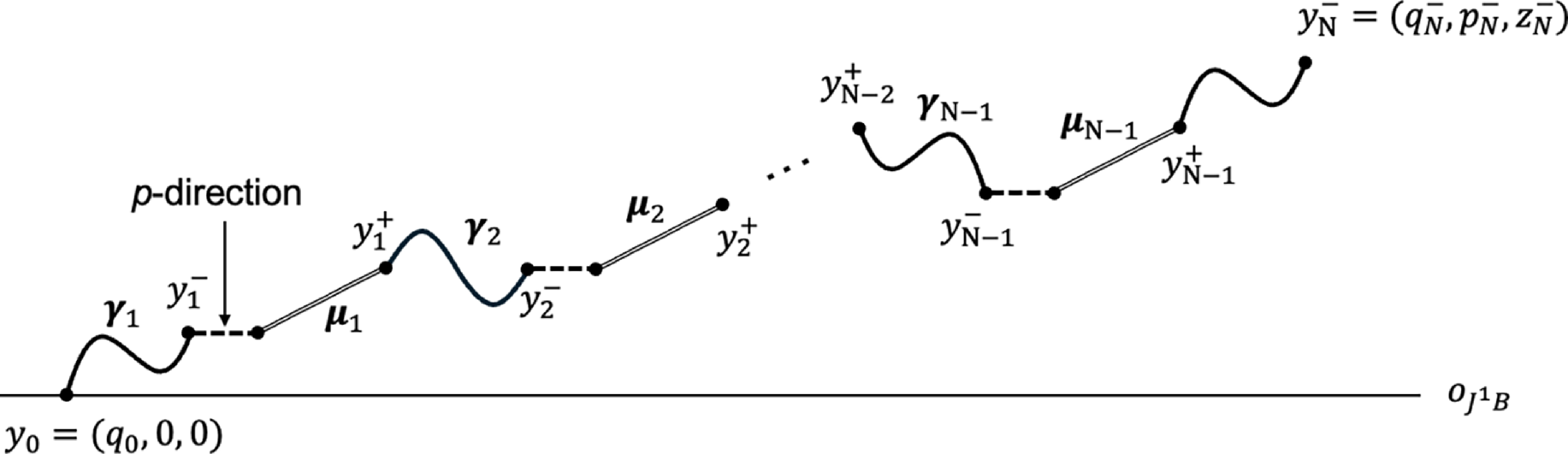
 J1B
 γk
 yk−1+
 yk−
 μk
 yk+
 γk
 μk
 y0=(q0,0,0)
 yN−=(qN−,pN−,zN−)

 Open access

