1 Introduction
Low-Reynolds-number locomotion has attracted considerable attention due to the fundamental importance of motility of micro-organisms in many biological processes (Fauci & Dillon Reference Fauci and Dillon2006; Lauga & Powers Reference Lauga and Powers2009). Improved understanding of the physics of swimming at small scales has also guided the design of synthetic micro-swimmers for various biomedical applications (Ebbens & Howse Reference Ebbens and Howse2010; Nelson, Kaliakatsos & Abbott Reference Nelson, Kaliakatsos and Abbott2010). Micro-organisms adopt a variety of mechanisms to overcome the constraints of swimming in the absence of inertia (Brennen & Winet Reference Brennen and Winet1977). Some micro-organisms, such as spermatozoa and bacteria, propel themselves by propagating travelling waves along their appendages (called flagella) by bending or rotating the flagella. Other micro-organisms, such as Volvox (Drescher et al. Reference Drescher, Leptos, Tuval, Ishikawa, Pedley and Goldstein2009) and Paramecium (Tamm Reference Tamm1972), have their surfaces covered with arrays of cilia (short flagella) and swim by beating these cilia in coordinated fashions.
Building upon pioneering works on flagellar swimming (Taylor Reference Taylor1951; Hancock Reference Hancock1953; Gray & Hancock Reference Gray and Hancock1955) and ciliary propulsion (Lighthill Reference Lighthill1952; Blake Reference Blake1971), the hydrodynamics of swimming micro-organisms in viscous media is relatively well studied (Lauga & Powers Reference Lauga and Powers2009). However, micro-organisms often encounter heterogeneous viscous environments consisting of networks of obstacles embedded into viscous fluid media. For instance, spermatozoa navigate through cervical mucus with a filamentous network (Rutllant, Lopez-Bejar & Lopez-Gatius Reference Rutllant, Lopez-Bejar and Lopez-Gatius2005); some spirochetes swim through highly complex and heterogeneous media and cross the blood–brain barrier to infect the brain (Radolf & Lukehart Reference Radolf and Lukehart2006; Wolgemuth Reference Wolgemuth2015); bacteria Helicobacter pylori can invade the epithelial cells by moving through the gastric mucus gel that protects the stomach (Celli et al. Reference Celli, Turner, Afdhal, Keates, Ghiran, Kelly, Ewoldt, McKinley, So, Erramilli and Bansil2009; Mirbagheri & Fu Reference Mirbagheri and Fu2016); and some bacteria and nematodes live in saturated soil in nature (Jung Reference Jung2010; Tecon & Or Reference Tecon and Or2016). An understanding of the effects due to networks of obstacles on locomotion is still developing (Berg & Turner Reference Berg and Turner1979; Siddiqui & Ansari Reference Siddiqui and Ansari2003; Leshansky Reference Leshansky2009; Fu, Shenoy & Powers Reference Fu, Shenoy and Powers2010; Jung Reference Jung2010; Jabbarzadeh, Hyon & Fu Reference Jabbarzadeh, Hyon and Fu2014; Ho & Olson Reference Ho and Olson2016; Leiderman & Olson Reference Leiderman and Olson2016; Mirbagheri & Fu Reference Mirbagheri and Fu2016).
The presence of a sparse network of stationary obstacles embedded into a viscous, incompressible Newtonian flow can be modelled by an effective medium approach to obtain the Brinkman equation (Brinkman Reference Brinkman1949)
 $$\begin{eqnarray}\unicode[STIX]{x1D707}\unicode[STIX]{x1D6FB}^{2}\boldsymbol{u}-\unicode[STIX]{x1D735}p-\unicode[STIX]{x1D707}\unicode[STIX]{x1D6FC}^{2}\boldsymbol{u}=\mathbf{0},\quad \unicode[STIX]{x1D735}\boldsymbol{\cdot }\boldsymbol{u}=0,\end{eqnarray}$$
which includes the additional hydrodynamic resistance
 $-\unicode[STIX]{x1D707}\unicode[STIX]{x1D6FC}^{2}\boldsymbol{u}$
due to the network of stationary obstacles. Here,
 $\unicode[STIX]{x1D707}$
is the fluid viscosity,
 $\unicode[STIX]{x1D6FC}^{-2}$
is the permeability, and
 $\boldsymbol{u}$
and
 $p$
are the average velocity and pressure fields, respectively. Although the Brinkman equation was introduced as a phenomenological model, its validity at low particle volume fraction was established by proper averaging methods (Tam Reference Tam1969; Childress Reference Childress1972; Howells Reference Howells1974; Hinch Reference Hinch1977). Numerical simulations also showed that the Brinkman equation still captures the qualitative behaviour even for moderately concentrated porous media (Durlofsky & Brady Reference Durlofsky and Brady1987).
The Brinkman equation has been employed to address the effects of viscous heterogeneous environment on locomotion performance. Leshansky (Reference Leshansky2009) considered the propulsion of an infinite waving sheet with transverse distortions and a rotating helical filament, and showed that the propulsion speed and swimming efficiency of these swimmers are always enhanced compared with swimming in a purely viscous medium. Experiments and modelling on locomotion of nematodes in wet particulate media also found greater distances travelled per undulation compared with the case without particles (Jung Reference Jung2010). However, the presence of obstacles does not always enhance locomotion performance. The propulsion speed of an infinite waving sheet propagating a longitudinal travelling wave was shown to remain unaffected but the propulsion efficiency is diminished (Leshansky Reference Leshansky2009). Recently, Ho & Olson (Reference Ho and Olson2016) performed asymptotic calculations for an infinite waving cylindrical tail with lateral and spiral displacements in a Brinkman fluid and studied finite-length swimmers numerically using the method of regularized Brinkmanlets (Cortez et al. Reference Cortez, Cummins, Leiderman and Varela2010). It was found that the swimming speed of these swimmers can be enhanced for specific combinations of permeability and geometric parameters of the swimmer. When the kinematics of the swimmer is not prescribed but emerges as a result of fluid–structure interactions, the propulsion speed and efficiency display non-monotonic variations with permeability (Leiderman & Olson Reference Leiderman and Olson2016). As a remark, while many studies (including the present work) treat the embedded obstacles as a stationary network, the effect of network deformability on locomotion has also been considered by modelling the network and solvent as two coupled elastic and viscous continuum phases (Fu et al. Reference Fu, Shenoy and Powers2010).
In addition to flagellated swimmers described above, propulsion of ciliates (such as Volvox and Paramecium) in heterogeneous viscous media has also been considered via the squirmer model by Leshansky (Reference Leshansky2009). Squirmers were first studied by Lighthill (Reference Lighthill1952) and Blake (Reference Blake1971) as idealized models for ciliary propulsion, where the beating of cilia is represented by surface velocities on the spherical cell body (Pedley Reference Pedley2016). The squirmer model has become popular as a general locomotion model because the surface velocities can be adjusted to represent different types of swimmers in the far field (Ishikawa, Simmonds & Pedley Reference Ishikawa, Simmonds and Pedley2006; Drescher, Goldstein & Tuval Reference Drescher, Goldstein and Tuval2010; Michelin & Lauga Reference Michelin and Lauga2011; Doostmohammadi, Stocker & Ardekani Reference Doostmohammadi, Stocker and Ardekani2012; Wang & Ardekani Reference Wang and Ardekani2012; Zöttl & Stark Reference Zöttl and Stark2012; Yazdi, Ardekani & Borhan Reference Yazdi, Ardekani and Borhan2015; Chisholm et al. Reference Chisholm, Legendre, Lauga and Khair2016). Stone & Samuel (Reference Stone and Samuel1996) applied the reciprocal theorem (Happel & Brenner Reference Happel and Brenner1973) to calculate the propulsion speed of a squirmer in a Newtonian fluid without knowledge of the surrounding flow. Leshansky (Reference Leshansky2009) adopted the same approach to calculate the propulsion speed of a squirmer in a Brinkman medium. The reciprocal theorem approach, however, cannot get as far regarding the calculation of power dissipation, which involves gradients of the surrounding flow. The power dissipation and swimming efficiency of a squirmer therefore can only be determined when the flow surrounding the squirmer is known. An analytical solution of the flow around a squirmer was obtained by Lighthill (Reference Lighthill1952) and Blake (Reference Blake1971) in Stokes flows, but the solution remains unknown in Brinkman flows. The energetic cost and efficiency of squirming in porous media hence are not yet quantified. The lack of knowledge about the surrounding flow also prevents a general understanding of the flow structure and characteristics of swimming in heterogeneous viscous media.
In this work, we fill in the above missing information by extending the classical analyses by Lighthill (Reference Lighthill1952) and Blake (Reference Blake1971) on squirming motion in a purely viscous fluid to the case of a heterogeneous viscous medium. The geometrical simplicity of the squirmer model allows one of few exact solutions for locomotion problems in a Brinkman medium. We employ the solution to examine the modifications of the flow structure around a squirmer due to the presence of a network of stationary obstacles. Our results lay the foundation for subsequent studies on hydrodynamic interactions as well as nutrient transport and uptake by micro-organisms in heterogeneous viscous media (Magar, Goto & Pedley Reference Magar, Goto and Pedley2003; Michelin & Lauga Reference Michelin and Lauga2011).
The paper is organized as follows. We formulate the problem mathematically in § 2 before presenting the solution to two problems related to the squirming motion: the pumping problem (§ 3.1) and the swimming problem (§ 3.2). With knowledge of the flow field, we calculate and discuss the propulsion speed, power dissipation and swimming efficiency of a squirmer in a Brinkman medium (§ 3.2.2). In § 4, we analyse the flow structure of squirming in a Brinkman medium and compare with the corresponding Stokes flows, before some concluding remarks in § 5.
2 Formulation
2.1 The squirmer model
We consider a steady, spherical squirmer of radius
 $a$
with tangential surface velocity distribution decomposed into a series of Legendre polynomials of the form (Lighthill Reference Lighthill1952; Blake Reference Blake1971; Pedley Reference Pedley2016)
 $$\begin{eqnarray}\boldsymbol{u}(r=a)=\mathop{\sum }_{n=1}^{\infty }B_{n}V_{n}(\cos \unicode[STIX]{x1D703})\boldsymbol{e}_{\unicode[STIX]{x1D703}},\end{eqnarray}$$
where
 $V_{n}=-2P_{n}^{1}(\cos \unicode[STIX]{x1D703})/[n(n+1)]$
,
 $P_{n}^{1}(\cos \unicode[STIX]{x1D703})$
represents an associated Legendre function of the first kind, and
 $\unicode[STIX]{x1D703}$
is the polar angle measured from the axis of symmetry. For squirming motion in Stokes flow, the
 $B_{n}$
modes can be related to Stokes singularity solutions. In particular, the
 $B_{1}$
mode corresponds to a source dipole in Stokes flows and is the only mode contributing to propulsion. The
 $B_{2}$
mode, corresponding to a Stokes force dipole, is the slowest decaying spatial mode and thus dominates the far-field velocity generated by the squirmer. Therefore, often only the first two modes,
 $B_{1}$
and
 $B_{2}$
, of the series are considered in locomotion problems (Ishikawa & Hota Reference Ishikawa and Hota2006; Ishikawa & Pedley Reference Ishikawa and Pedley2008; Doostmohammadi et al.
Reference Doostmohammadi, Stocker and Ardekani2012; Wang & Ardekani Reference Wang and Ardekani2012; Zöttl & Stark Reference Zöttl and Stark2012; Li & Ardekani Reference Li and Ardekani2014; Datt et al.
Reference Datt, Zhu, Elfring and Pak2015; Yazdi et al.
Reference Yazdi, Ardekani and Borhan2015; Chisholm et al.
Reference Chisholm, Legendre, Lauga and Khair2016). Since the
 $B_{2}$
mode corresponds to the force dipole exerted on the fluid by the swimmer to generate propulsion, the relative signs of
 $B_{1}$
and
 $B_{2}$
modes can be adjusted to represent different types of swimmers (Pedley Reference Pedley2016). These include pushers (
 $\unicode[STIX]{x1D6FD}_{2}=B_{2}/B_{1}<0$
), which obtain their thrust from their rear (e.g. Escherichia coli), and pullers (
 $\unicode[STIX]{x1D6FD}_{2}>0$
), which obtain their thrust from their front (e.g. Chlamydomonas), and neutral squirmers (
 $\unicode[STIX]{x1D6FD}_{2}=0$
). Although squirmers with tangential surface velocities are more commonly studied in the literature (Pedley Reference Pedley2016), we also present results on squirming with radial surface velocities in appendix A for completeness.
2.2 Governing equation
The incompressible flow around a spherical squirmer in a heterogeneous viscous medium is modelled by the Brinkman equation (1.1). We non-dimensionalize lengths by the squirmer radius
 $a$
, velocities by the first mode of actuation
 $B_{1}$
, and pressure by
 $\unicode[STIX]{x1D707}B_{1}/a$
. The dimensionless Brinkman equation is given by
 $$\begin{eqnarray}-\unicode[STIX]{x1D735}^{\ast }p^{\ast }+\unicode[STIX]{x0394}^{\ast }\boldsymbol{u}^{\ast }-\unicode[STIX]{x1D6FF}^{2}\boldsymbol{u}^{\ast }=\mathbf{0},\quad \unicode[STIX]{x1D735}^{\ast }\boldsymbol{\cdot }\boldsymbol{u}^{\ast }=0,\end{eqnarray}$$
where the dimensionless group
 $\unicode[STIX]{x1D6FF}=a\unicode[STIX]{x1D6FC}$
compares the squirmer radius
 $a$
to the Brinkman screening length
 $\unicode[STIX]{x1D6FC}^{-1}$
. As
 $\unicode[STIX]{x1D6FF}$
approaches zero, the Brinkman equation reduces to the Stokes equation; for large
 $\unicode[STIX]{x1D6FF}$
, the equation reduces to the Darcy equation. Dimensionless variables are denoted by stars (
 $\ast$
) above. Henceforth we shall only work in dimensionless quantities unless otherwise stated and therefore drop the stars (
 $\ast$
) for convenience. With these non-dimensionalizations, the dimensionless tangential surface velocity distribution on a squirmer is given by
 $$\begin{eqnarray}\boldsymbol{u}(r=1)=\mathop{\sum }_{n=1}^{\infty }\unicode[STIX]{x1D6FD}_{n}V_{n}(\cos \unicode[STIX]{x1D703})\boldsymbol{e}_{\unicode[STIX]{x1D703}},\end{eqnarray}$$
where
 $\unicode[STIX]{x1D6FD}_{n}=B_{n}/B_{1}$
.
Owing to the axisymmetry of the problem, we can express the velocity flow field
 $\boldsymbol{u}=u\boldsymbol{e}_{r}+v\boldsymbol{e}_{\unicode[STIX]{x1D703}}$
in terms of the Stokes stream function (Happel & Brenner Reference Happel and Brenner1973),
 $$\begin{eqnarray}u=\frac{1}{r^{2}\sin \unicode[STIX]{x1D703}}\frac{\unicode[STIX]{x2202}\unicode[STIX]{x1D713}}{\unicode[STIX]{x2202}\unicode[STIX]{x1D703}},\quad v=-\frac{1}{r\sin \unicode[STIX]{x1D703}}\frac{\unicode[STIX]{x2202}\unicode[STIX]{x1D713}}{\unicode[STIX]{x2202}r},\end{eqnarray}$$
to satisfy the continuity equation. The dimensionless Brinkman equation (2.2) in terms of the Stokes streamfunction therefore becomes
 $$\begin{eqnarray}D^{2}(D^{2}-\unicode[STIX]{x1D6FF}^{2})\unicode[STIX]{x1D713}=0,\end{eqnarray}$$
where the operator
 $$\begin{eqnarray}D^{2}\equiv \frac{\unicode[STIX]{x2202}^{2}}{\unicode[STIX]{x2202}r^{2}}+\frac{\sin \unicode[STIX]{x1D703}}{r^{2}}\frac{\unicode[STIX]{x2202}}{\unicode[STIX]{x2202}\unicode[STIX]{x1D703}}\left(\frac{1}{\sin \unicode[STIX]{x1D703}}\frac{\unicode[STIX]{x2202}}{\unicode[STIX]{x2202}\unicode[STIX]{x1D703}}\right).\end{eqnarray}$$
By splitting the streamfunction into
 $\unicode[STIX]{x1D713}=\unicode[STIX]{x1D713}^{(1)}+\unicode[STIX]{x1D713}^{(2)}$
with
 $D^{2}\unicode[STIX]{x1D713}^{(1)}=0$
and
 $(D^{2}-\unicode[STIX]{x1D6FF}^{2})\unicode[STIX]{x1D713}^{(2)}=0$
, a general solution of (2.5) can be obtained via separation of variables as (Zlatanovski Reference Zlatanovski1999; Palaniappan Reference Palaniappan2014)
 $$\begin{eqnarray}\unicode[STIX]{x1D713}=\mathop{\sum }_{n=1}^{\infty }f_{n}(r)\sin \unicode[STIX]{x1D703}\,P_{n}^{1}(\cos \unicode[STIX]{x1D703}),\end{eqnarray}$$
where
 $$\begin{eqnarray}f_{n}(r)=\left\{C_{n}r^{-n}+D_{n}r^{n+1}+\frac{r^{1/2}}{\unicode[STIX]{x1D6FF}^{2}}[E_{n}\text{K}_{n+1/2}(\unicode[STIX]{x1D6FF}r)+F_{n}\text{I}_{n+1/2}(\unicode[STIX]{x1D6FF}r)]\right\},\end{eqnarray}$$
and
 $\text{I}_{n+1/2}(\unicode[STIX]{x1D6FF}r)$
and
 $\text{K}_{n+1/2}(\unicode[STIX]{x1D6FF}r)$
are, respectively, the modified Bessel functions of the first and second kinds. The coefficients
 $C_{n},~D_{n},~E_{n}$
and
 $F_{n}$
are determined from the boundary conditions in the following problems.
3 Squirming motion in a Brinkman medium
Owing to the linearity of the Stokes and Brinkman equations, we can decompose the locomotion problem into two separate steps, namely the pumping problem (§ 3.1) and the swimming problem (§ 3.2), to better illustrate the solution structure (Pak & Lauga Reference Pak and Lauga2014; Schmitt & Stark Reference Schmitt and Stark2016). In the first step – the pumping problem – the squirmer is not allowed to move but is held fixed in space by an external force. A net flow
 $\boldsymbol{u}_{P}$
is generated as a result of the surface actuation on the squirmer, (2.3); the squirmer acts as a pump in this case. In the second step – the swimming problem – the squirmer is allowed to move freely at a swimming velocity,
 $\boldsymbol{U}$
, which induces a flow due to the translational motion
 $\boldsymbol{u}_{T}$
. The overall flow field around a self-propelling squirmer
 $\boldsymbol{u}=\boldsymbol{u}_{P}+\boldsymbol{u}_{T}$
can then be considered as a superposition of the solution of the pumping problem and the flow field due to the induced translation.
3.1 Pumping problem
We employ the general solution (2.7) with (2.8) to determine the flow generated by a squirmer held fixed in the pumping problem,
 $\boldsymbol{u}_{P}$
. In the laboratory frame, the flow in the far field (
 $r\rightarrow \infty$
) decays to zero, which demands the growing terms in (2.8) to vanish, i.e.
 $D_{n}=F_{n}=0$
for
 $n\geqslant 1$
. At the surface of the squirmer (
 $r=1$
), we require the radial velocity
 $u$
to vanish and the tangential surface velocity distribution
 $v$
to match with that in (2.3). In terms of the Stokes streamfunction, these conditions are given by
 $$\begin{eqnarray}\displaystyle & \displaystyle C_{n}+\frac{\text{K}_{n+1/2}(\unicode[STIX]{x1D6FF})}{\unicode[STIX]{x1D6FF}^{2}}E_{n}=0, & \displaystyle\end{eqnarray}$$
 $$\begin{eqnarray}\displaystyle & \displaystyle -nC_{n}+\left[\frac{\text{K}_{n+1/2}(\unicode[STIX]{x1D6FF})}{2\unicode[STIX]{x1D6FF}^{2}}-\frac{\text{K}_{n-1/2}(\unicode[STIX]{x1D6FF})+\text{K}_{n+3/2}(\unicode[STIX]{x1D6FF})}{2\unicode[STIX]{x1D6FF}}\right]E_{n}=-\frac{2}{n(n+1)}\unicode[STIX]{x1D6FD}_{n}, & \displaystyle\end{eqnarray}$$
respectively. The system of (3.1) and (3.2) is solved to obtain the coefficients
 $$\begin{eqnarray}\left.\begin{array}{@{}c@{}}\displaystyle C_{n}=\frac{4\text{K}_{n+1/2}(\unicode[STIX]{x1D6FF})\unicode[STIX]{x1D6FD}_{n}}{n(n+1)[-\unicode[STIX]{x1D6FF}\text{K}_{n-1/2}(\unicode[STIX]{x1D6FF})+(1+2n)\text{K}_{n+1/2}(\unicode[STIX]{x1D6FF})-\unicode[STIX]{x1D6FF}\text{K}_{n+3/2}(\unicode[STIX]{x1D6FF})]},\\ \displaystyle E_{n}=\frac{-4\unicode[STIX]{x1D6FF}^{2}\unicode[STIX]{x1D6FD}_{n}}{n(n+1)[-\unicode[STIX]{x1D6FF}\text{K}_{n-1/2}(\unicode[STIX]{x1D6FF})+(1+2n)\text{K}_{n+1/2}(\unicode[STIX]{x1D6FF})-\unicode[STIX]{x1D6FF}\text{K}_{n+3/2}(\unicode[STIX]{x1D6FF})]}.\end{array}\right\}\end{eqnarray}$$
Upon substitution of these coefficients into the streamfunction, the flow field in the pumping problem
 $\boldsymbol{u}_{P}=u_{P}\boldsymbol{e}_{r}+v_{P}\boldsymbol{e}_{\unicode[STIX]{x1D703}}$
is determined as
 $$\begin{eqnarray}\displaystyle u_{P} & = & \displaystyle \frac{2[\text{e}^{\unicode[STIX]{x1D6FF}-r\unicode[STIX]{x1D6FF}}(1+r\unicode[STIX]{x1D6FF})-(1+\unicode[STIX]{x1D6FF})]}{r^{3}\unicode[STIX]{x1D6FF}^{2}}\cos \unicode[STIX]{x1D703}\nonumber\\ \displaystyle & & \displaystyle +\,\mathop{\sum }_{n=2}^{\infty }\frac{4r^{-2-n}\unicode[STIX]{x1D6FD}_{n}[\text{K}_{n+1/2}(\unicode[STIX]{x1D6FF})-r^{n+1/2}\text{K}_{n+1/2}(r\unicode[STIX]{x1D6FF})]P_{n}(\cos \unicode[STIX]{x1D703})}{[-\unicode[STIX]{x1D6FF}\text{K}_{n-1/2}(\unicode[STIX]{x1D6FF})+(1+2n)\text{K}_{n+1/2}(\unicode[STIX]{x1D6FF})-\unicode[STIX]{x1D6FF}\text{K}_{n+3/2}(\unicode[STIX]{x1D6FF})]},\end{eqnarray}$$
 $$\begin{eqnarray}\displaystyle v_{P} & = & \displaystyle \frac{\text{e}^{\unicode[STIX]{x1D6FF}-r\unicode[STIX]{x1D6FF}}(1+r\unicode[STIX]{x1D6FF}+r^{2}\unicode[STIX]{x1D6FF}^{2})-(1+\unicode[STIX]{x1D6FF})}{r^{3}\unicode[STIX]{x1D6FF}^{2}}\sin \unicode[STIX]{x1D703}\nonumber\\ \displaystyle & & \displaystyle +\,\mathop{\sum }_{n=2}^{\infty }\frac{-r^{-2-n}\unicode[STIX]{x1D6FD}_{n}V_{n}(\cos \unicode[STIX]{x1D703})}{[-\unicode[STIX]{x1D6FF}\text{K}_{n-1/2}(\unicode[STIX]{x1D6FF})+(1+2n)\text{K}_{n+1/2}(\unicode[STIX]{x1D6FF})-\unicode[STIX]{x1D6FF}\text{K}_{n+3/2}(\unicode[STIX]{x1D6FF})]}\nonumber\\ \displaystyle & & \displaystyle \times \,[-2n\text{K}_{n+1/2}(\unicode[STIX]{x1D6FF})+\unicode[STIX]{x1D6FF}r^{n+3/2}\text{K}_{n-1/2}(r\unicode[STIX]{x1D6FF})-r^{n+1/2}\text{K}_{n+1/2}(r\unicode[STIX]{x1D6FF})+\unicode[STIX]{x1D6FF}r^{n+3/2}\text{K}_{n+3/2}(r\unicode[STIX]{x1D6FF})].\nonumber\\ \displaystyle & & \displaystyle\end{eqnarray}$$
For the special case of a two-mode squirmer commonly studied in the literature (Pedley Reference Pedley2016), the above solution reduces to
 $\boldsymbol{u}_{P}=\boldsymbol{u}_{P,B_{1}}+\unicode[STIX]{x1D6FD}_{2}\boldsymbol{u}_{P,B_{2}}$
, where
 $$\begin{eqnarray}\boldsymbol{u}_{P,B_{1}}=\frac{2[\text{e}^{\unicode[STIX]{x1D6FF}-r\unicode[STIX]{x1D6FF}}(1+r\unicode[STIX]{x1D6FF})-(1+\unicode[STIX]{x1D6FF})]}{\unicode[STIX]{x1D6FF}^{2}r^{3}}\cos \unicode[STIX]{x1D703}\,\boldsymbol{e}_{r}+\frac{\text{e}^{\unicode[STIX]{x1D6FF}-r\unicode[STIX]{x1D6FF}}(1+r\unicode[STIX]{x1D6FF}+r^{2}\unicode[STIX]{x1D6FF}^{2})-(1+\unicode[STIX]{x1D6FF})}{\unicode[STIX]{x1D6FF}^{2}r^{3}}\sin \unicode[STIX]{x1D703}\,\boldsymbol{e}_{\unicode[STIX]{x1D703}},\end{eqnarray}$$
 $$\begin{eqnarray}\displaystyle \boldsymbol{u}_{P,B_{2}} & = & \displaystyle \frac{\text{e}^{\unicode[STIX]{x1D6FF}-r\unicode[STIX]{x1D6FF}}(3+3r\unicode[STIX]{x1D6FF}+r^{2}\unicode[STIX]{x1D6FF}^{2})-(3+3\unicode[STIX]{x1D6FF}+\unicode[STIX]{x1D6FF}^{2})}{2\unicode[STIX]{x1D6FF}^{2}(1+\unicode[STIX]{x1D6FF})r^{4}}[1+3\cos (2\unicode[STIX]{x1D703})]\boldsymbol{e}_{r}\nonumber\\ \displaystyle & & \displaystyle +\,\frac{\text{e}^{\unicode[STIX]{x1D6FF}-r\unicode[STIX]{x1D6FF}}(6+6r\unicode[STIX]{x1D6FF}+3r^{2}\unicode[STIX]{x1D6FF}^{2}+r^{3}\unicode[STIX]{x1D6FF}^{3})-2(3+3\unicode[STIX]{x1D6FF}+\unicode[STIX]{x1D6FF}^{2})}{2\unicode[STIX]{x1D6FF}^{2}(1+\unicode[STIX]{x1D6FF})r^{4}}\sin (2\unicode[STIX]{x1D703})\boldsymbol{e}_{\unicode[STIX]{x1D703}}.\end{eqnarray}$$
The structure of the flow given by (3.6) and (3.7) in the pumping problem will be studied in terms of singularities in Brinkman flows in § 4.
3.2 Swimming problem
When the squirmer is allowed to move freely, the overall flow field
 $\boldsymbol{u}=\boldsymbol{u}_{P}+\boldsymbol{u}_{T}$
has an additional component
 $\boldsymbol{u}_{T}$
due to the translation of the spherical body at the unknown swimming speed
 $U$
in a Brinkman medium. The exact solution to this translational problem is given by (Howells Reference Howells1974)
 $$\begin{eqnarray}\displaystyle \boldsymbol{u}_{T} & = & \displaystyle U\cos \unicode[STIX]{x1D703}\left[\frac{3+3\unicode[STIX]{x1D6FF}+\unicode[STIX]{x1D6FF}^{2}-3\text{e}^{\unicode[STIX]{x1D6FF}-\unicode[STIX]{x1D6FF}r}(1+r\unicode[STIX]{x1D6FF})}{r^{3}\unicode[STIX]{x1D6FF}^{2}}\right]\boldsymbol{e}_{r}\nonumber\\ \displaystyle & & \displaystyle +\,U\sin \unicode[STIX]{x1D703}\left[\frac{3+3\unicode[STIX]{x1D6FF}+\unicode[STIX]{x1D6FF}^{2}-3\text{e}^{\unicode[STIX]{x1D6FF}-\unicode[STIX]{x1D6FF}r}(1+r\unicode[STIX]{x1D6FF}+r^{2}\unicode[STIX]{x1D6FF}^{2})}{2r^{3}\unicode[STIX]{x1D6FF}^{2}}\right]\boldsymbol{e}_{\unicode[STIX]{x1D703}}.\end{eqnarray}$$
The unknown swimming speed
 $U$
in the overall flow field
 $\boldsymbol{u}=\boldsymbol{u}_{P}+\boldsymbol{u}_{T}$
, where
 $\boldsymbol{u}_{P}$
is given by (3.4) and (3.5), is then determined by enforcing the force-free condition on the squirmer,
 $$\begin{eqnarray}\int _{S}\unicode[STIX]{x1D64F}\boldsymbol{\cdot }\boldsymbol{n}\,\text{d}S=\mathbf{0},\end{eqnarray}$$
where the dimensionless stress
 $\unicode[STIX]{x1D64F}=-p\unicode[STIX]{x1D644}+\dot{\unicode[STIX]{x1D738}}$
and the rate-of-strain tensor
 $\dot{\unicode[STIX]{x1D738}}=\unicode[STIX]{x1D735}\boldsymbol{u}+(\unicode[STIX]{x1D735}\boldsymbol{u})^{\text{T}}$
. The force-free condition (3.9) therefore leads to a propulsion speed
 $$\begin{eqnarray}U=\frac{6(1+\unicode[STIX]{x1D6FF})}{9+9\unicode[STIX]{x1D6FF}+\unicode[STIX]{x1D6FF}^{2}},\end{eqnarray}$$
which agrees with the results obtained by Leshansky (Reference Leshansky2009) via the reciprocal theorem. The swimming speed (3.10) in dimensional form reads
 $\tilde{U} =6(1+\unicode[STIX]{x1D6FF})B_{1}/(9+9\unicode[STIX]{x1D6FF}+\unicode[STIX]{x1D6FF}^{2})$
. Similar to squirming in Stokes flows, only the
 $B_{1}$
mode out of all squirming modes in (2.3) contributes to propulsion. The propulsion speed monotonically decreases with increasing
 $\unicode[STIX]{x1D6FF}$
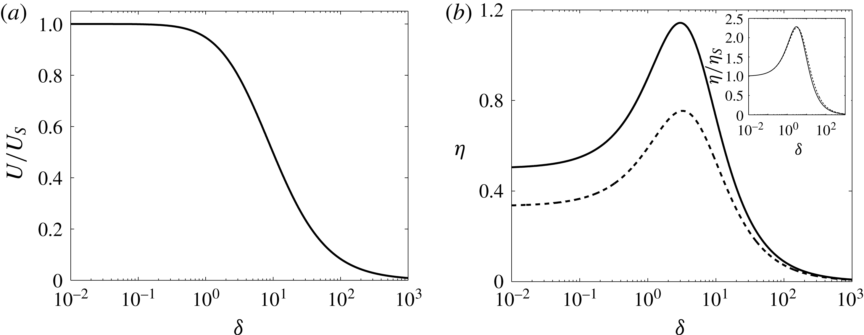
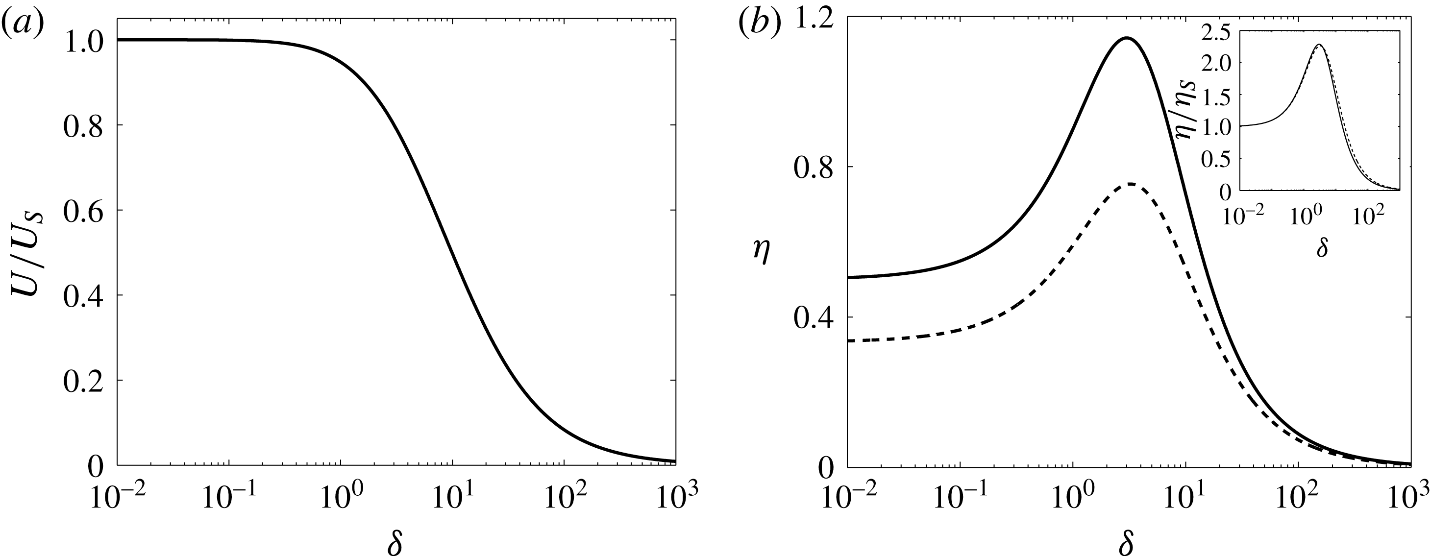
as shown in figure 2(a).
3.2.1 Flow around a squirmer in a Brinkman medium
The use of the reciprocal theorem is effective in bypassing calculations of the flow field to obtain the swimming speed. However, information such as power dissipation, swimming efficiency and nutrient uptake of the squirmer cannot be obtained without knowledge of the flow around the squirmer. Here we fill in this missing information by substituting the swimming speed (3.10) into the overall flow
 $\boldsymbol{u}=\boldsymbol{u}_{P}+\boldsymbol{u}_{T}$
and obtain an analytical solution for the flow around a squirmer in a Brinkman medium,
 $$\begin{eqnarray}\displaystyle u & = & \displaystyle \frac{[4(1+\unicode[STIX]{x1D6FF})+2\text{e}^{\unicode[STIX]{x1D6FF}-r\unicode[STIX]{x1D6FF}}(1+r\unicode[STIX]{x1D6FF})]\cos \unicode[STIX]{x1D703}}{r^{3}(9+9\unicode[STIX]{x1D6FF}+\unicode[STIX]{x1D6FF}^{2})}\nonumber\\ \displaystyle & & \displaystyle +\,\mathop{\sum }_{n=2}^{\infty }\frac{4r^{-2-n}\unicode[STIX]{x1D6FD}_{n}[\text{K}_{n+1/2}(\unicode[STIX]{x1D6FF})-r^{n+1/2}\text{K}_{n+1/2}(r\unicode[STIX]{x1D6FF})]P_{n}(\cos \unicode[STIX]{x1D703})}{[-\unicode[STIX]{x1D6FF}\text{K}_{n-1/2}(\unicode[STIX]{x1D6FF})+(1+2n)\text{K}_{n+1/2}(\unicode[STIX]{x1D6FF})-\unicode[STIX]{x1D6FF}\text{K}_{n+3/2}(\unicode[STIX]{x1D6FF})]},\end{eqnarray}$$
 $$\begin{eqnarray}\displaystyle v & = & \displaystyle \frac{[2(1+\unicode[STIX]{x1D6FF})+\text{e}^{\unicode[STIX]{x1D6FF}-r\unicode[STIX]{x1D6FF}}(1+r\unicode[STIX]{x1D6FF}+r^{2}\unicode[STIX]{x1D6FF}^{2})]\sin \unicode[STIX]{x1D703}}{r^{3}(9+9\unicode[STIX]{x1D6FF}+\unicode[STIX]{x1D6FF}^{2})}\nonumber\\ \displaystyle & & \displaystyle +\,\mathop{\sum }_{n=2}^{\infty }\frac{-r^{-2-n}\unicode[STIX]{x1D6FD}_{n}V_{n}(\cos \unicode[STIX]{x1D703})}{[-\unicode[STIX]{x1D6FF}\text{K}_{n-1/2}(\unicode[STIX]{x1D6FF})+(1+2n)\text{K}_{n+1/2}(\unicode[STIX]{x1D6FF})-\unicode[STIX]{x1D6FF}\text{K}_{n+3/2}(\unicode[STIX]{x1D6FF})]}\nonumber\\ \displaystyle & & \displaystyle \times \,[-2n\text{K}_{n+1/2}(\unicode[STIX]{x1D6FF})+\unicode[STIX]{x1D6FF}r^{n+3/2}\text{K}_{n-1/2}(r\unicode[STIX]{x1D6FF})-r^{n+1/2}\text{K}_{n+1/2}(r\unicode[STIX]{x1D6FF})+\unicode[STIX]{x1D6FF}r^{n+3/2}\text{K}_{n+3/2}(r\unicode[STIX]{x1D6FF})].\nonumber\\ \displaystyle & & \displaystyle\end{eqnarray}$$
In particular, for a two-mode squirmer the solution reduces to
 $\boldsymbol{u}=\boldsymbol{u}_{B_{1}}+\unicode[STIX]{x1D6FD}_{2}\boldsymbol{u}_{B_{2}}$
, where
 $$\begin{eqnarray}\boldsymbol{u}_{B_{1}}=\frac{[4(1+\unicode[STIX]{x1D6FF})+2\text{e}^{\unicode[STIX]{x1D6FF}-r\unicode[STIX]{x1D6FF}}(1+r\unicode[STIX]{x1D6FF})]\cos \unicode[STIX]{x1D703}}{r^{3}(9+9\unicode[STIX]{x1D6FF}+\unicode[STIX]{x1D6FF}^{2})}\,\boldsymbol{e}_{r}+\frac{[2(1+\unicode[STIX]{x1D6FF})+\text{e}^{\unicode[STIX]{x1D6FF}-r\unicode[STIX]{x1D6FF}}(1+r\unicode[STIX]{x1D6FF}+r^{2}\unicode[STIX]{x1D6FF}^{2})]\sin \unicode[STIX]{x1D703}}{r^{3}(9+9\unicode[STIX]{x1D6FF}+\unicode[STIX]{x1D6FF}^{2})}\boldsymbol{e}_{\unicode[STIX]{x1D703}},\end{eqnarray}$$
 $$\begin{eqnarray}\displaystyle \boldsymbol{u}_{B_{2}} & = & \displaystyle \boldsymbol{u}_{P,B_{2}}\nonumber\\ \displaystyle & = & \displaystyle \frac{\text{e}^{\unicode[STIX]{x1D6FF}-r\unicode[STIX]{x1D6FF}}(3+3r\unicode[STIX]{x1D6FF}+r^{2}\unicode[STIX]{x1D6FF}^{2})-(3+3\unicode[STIX]{x1D6FF}+\unicode[STIX]{x1D6FF}^{2})}{2\unicode[STIX]{x1D6FF}^{2}(1+\unicode[STIX]{x1D6FF})r^{4}}[1+3\cos (2\unicode[STIX]{x1D703})]\boldsymbol{e}_{r}\nonumber\\ \displaystyle & & \displaystyle +\,\frac{\text{e}^{\unicode[STIX]{x1D6FF}-r\unicode[STIX]{x1D6FF}}(6+6r\unicode[STIX]{x1D6FF}+3r^{2}\unicode[STIX]{x1D6FF}^{2}+r^{3}\unicode[STIX]{x1D6FF}^{3})-2(3+3\unicode[STIX]{x1D6FF}+\unicode[STIX]{x1D6FF}^{2})}{2\unicode[STIX]{x1D6FF}^{2}(1+\unicode[STIX]{x1D6FF})r^{4}}\sin (2\unicode[STIX]{x1D703})\boldsymbol{e}_{\unicode[STIX]{x1D703}}.\end{eqnarray}$$
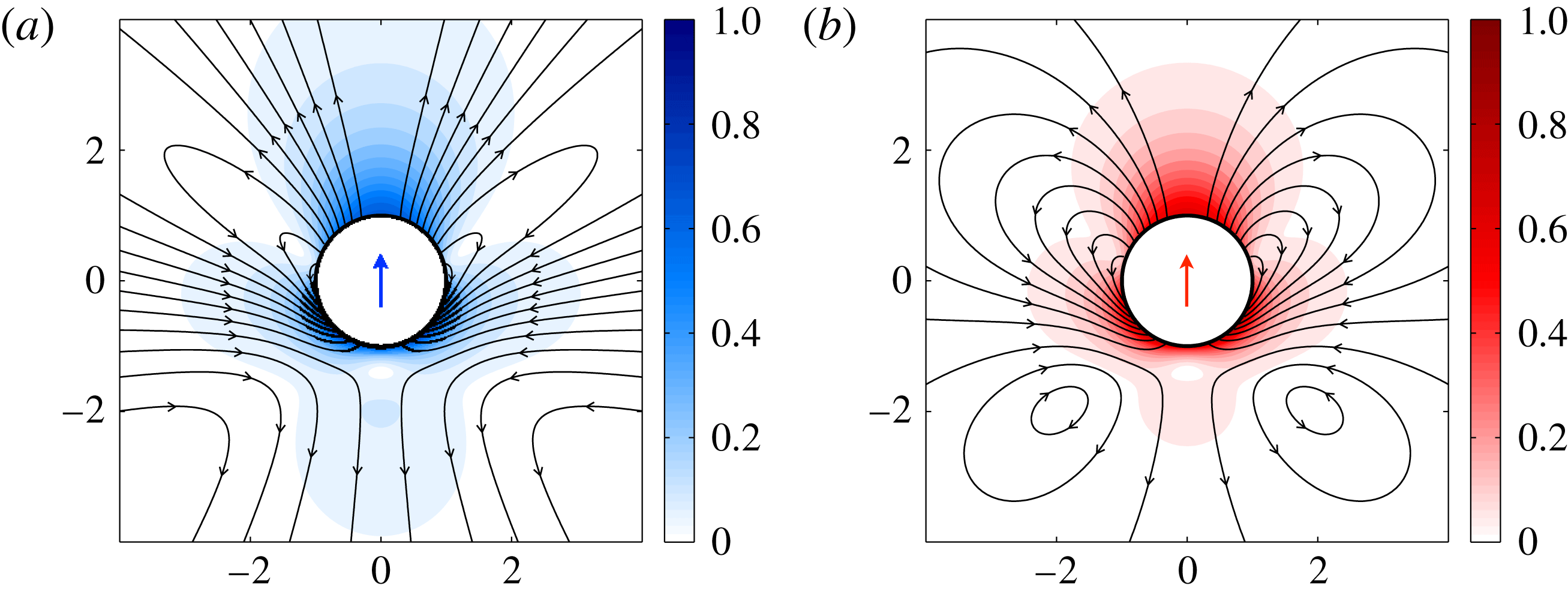
The presence of a network of obstacles alters the flow features around the squirmer. We plot in figure 1(b) the flow surrounding a self-propelling squirmer with
 $\unicode[STIX]{x1D6FD}_{2}=-1$
(a pusher) in a Brinkman medium in contrast to the Stokes case (figure 1
a). We remark that the flow due to the second mode is the same in the pumping and swimming problems because this mode has no contribution to swimming motion (Pak & Lauga Reference Pak and Lauga2014; Pedley Reference Pedley2016). We will analyse the structure of the flow given by (3.13) and (3.14) in the swimming problem in terms of singularities in Brinkman flows in § 4.
Streamlines and local speed of the dimensionless flow surrounding a self-propelling squirmer in (a) Stokes and (b) Brinkman flows with
 $\unicode[STIX]{x1D6FD}_{2}=-1$
(a pusher). The dimensionless resistance
 $\unicode[STIX]{x1D6FF}=1$
. The arrows on the squirmers indicate the swimming direction and the colour represents the magnitude of local flow velocity. The streamlines of a puller (
 $\unicode[STIX]{x1D6FD}_{2}=1$
) can be readily obtained by an upside-down flipping of the streamlines of the corresponding pusher about the horizontal axis. The presence of a network of obstacles alters the flow features around the squirmer. The flow structure and far-field behaviours are discussed in § 4.

3.2.2 Power dissipation and swimming efficiency
While swimming speed is an important property of locomotion, efficiency is another measure of performance that a swimmer may maximize to move through a medium in an energetically favourable manner. It is therefore biologically relevant to investigate how the properties of a swimmer and its surrounding medium influence the efficiency of locomotion. The classical definition of thermodynamic efficiency was proved difficult to apply in swimming at low Reynolds number (Childress Reference Childress2012). Lighthill introduced the Froude efficiency, a concept coming from propeller theory, to characterize the efficiency of low-Reynolds-number swimmers (Lighthill Reference Lighthill1952, Reference Lighthill1975). The swimming efficiency is defined as
 $$\begin{eqnarray}\unicode[STIX]{x1D702}=\frac{F_{D}U}{{\mathcal{P}}},\end{eqnarray}$$
which compares the total power dissipation
 ${\mathcal{P}}$
in the fluid during the swimming motion with a useful power output
 $F_{D}U$
, defined as the power against the drag
 $F_{D}$
in moving a rigid body of identical shape as the swimmer at the swimming speed
 $U$
. This standard definition has been widely adopted to characterize the efficiency of different low-Reynolds-number swimmers (Childress Reference Childress1981; Stone & Samuel Reference Stone and Samuel1996; Chattopadhyay et al.
Reference Chattopadhyay, Moldovan, Yeung and Wu2006; Leshansky et al.
Reference Leshansky, Kenneth, Gat and Avron2007; Tam & Hosoi Reference Tam and Hosoi2007; Michelin & Lauga Reference Michelin and Lauga2010; Ishimoto & Gaffney Reference Ishimoto and Gaffney2014; Wiezel & Or Reference Wiezel and Or2016).
Propulsion performance of a squirmer in a Brinkman medium. (a) Swimming speed
 $U$
scaled by the corresponding Stokes case
 $U_{S}$
as a function of dimensionless resistance
 $\unicode[STIX]{x1D6FF}$
. (b) Swimming efficiency
 $\unicode[STIX]{x1D702}$
of a neutral squirmer (
 $\unicode[STIX]{x1D6FD}_{2}=B_{2}/B_{1}=0$
, solid line) and a puller/pusher (
 $\unicode[STIX]{x1D6FD}_{2}=\pm 1$
, both represented by the dashed line) in a Brinkman medium. Inset: Swimming efficiency scaled by the corresponding Stokes case
 $\unicode[STIX]{x1D702}_{S}$
.
In a Brinkman medium, the drag experienced by a sphere translating at speed
 $U$
is given by (Howells Reference Howells1974; Leshansky Reference Leshansky2009; Cortez et al.
Reference Cortez, Cummins, Leiderman and Varela2010)
 $$\begin{eqnarray}F_{D}=6\unicode[STIX]{x03C0}\left(1+\unicode[STIX]{x1D6FF}+\frac{\unicode[STIX]{x1D6FF}^{2}}{9}\right)U,\end{eqnarray}$$
and the swimming speed is given by (3.10). We remark that in Stokes flows, the drag on a sphere is the same whether the sphere is translating in a quiescent flow or there is a uniform flow past a stationary sphere. However, in Brinkman flows, the drag in these two scenarios are different because there is a finite pressure gradient at infinity for a uniform flow due to the additional resistance in the Brinkman equation (Feng, Ganatos & Weinbaum Reference Feng, Ganatos and Weinbaum1998; Cortez et al.
Reference Cortez, Cummins, Leiderman and Varela2010). The pressure gradient induces a greater drag on the sphere for the case of a uniform flow past a stationary sphere, which is given by
 $6\unicode[STIX]{x03C0}(1+\unicode[STIX]{x1D6FF}+\unicode[STIX]{x1D6FF}^{2}/3)U$
. Since we are considering the motion of an active particle, we follow Leshansky (Reference Leshansky2009) and use the drag on a translating sphere here. The calculation of power dissipation
 ${\mathcal{P}}=-\int \unicode[STIX]{x1D64F}\boldsymbol{\cdot }\boldsymbol{n}\boldsymbol{\cdot }\boldsymbol{u}\,\text{d}S$
requires detailed information of the flow around a squirmer
 $\boldsymbol{u}$
and its gradients. We employ the solution given by (3.13) and (3.14) to derive the power dissipation of a two-mode squirmer as
 $$\begin{eqnarray}{\mathcal{P}}=\frac{8\unicode[STIX]{x03C0}}{15}\left[\frac{5(18+18\unicode[STIX]{x1D6FF}+3\unicode[STIX]{x1D6FF}^{2}+\unicode[STIX]{x1D6FF}^{3})}{9+9\unicode[STIX]{x1D6FF}+\unicode[STIX]{x1D6FF}^{2}}+\frac{(5+5\unicode[STIX]{x1D6FF}+\unicode[STIX]{x1D6FF}^{2})\unicode[STIX]{x1D6FD}_{2}^{2}}{1+\unicode[STIX]{x1D6FF}}\right]\!,\end{eqnarray}$$
which reduces to the results by Lighthill (Reference Lighthill1952) and Blake (Reference Blake1971) in Stokes flow,
 ${\mathcal{P}}_{S}=8\unicode[STIX]{x03C0}(2+\unicode[STIX]{x1D6FD}_{2}^{2})/3$
, in the limit of
 $\unicode[STIX]{x1D6FF}\rightarrow 0$
. Alternatively, one can also calculate the power dissipation
 ${\mathcal{P}}$
by summing the viscous dissipation and rate of work done on the flow by the Brinkman term, which gives the same result as (3.17).
We first probe the asymptotic behaviour of power output
 $F_{D}U$
and power dissipation
 ${\mathcal{P}}$
in small
 $\unicode[STIX]{x1D6FF}$
for a neutral squirmer as an illustration. The power output scales linearly with
 $\unicode[STIX]{x1D6FF}$
as
 $F_{D}U\sim 8\unicode[STIX]{x03C0}/3(1+\unicode[STIX]{x1D6FF})$
, while the power dissipation increases only quadratically as
 ${\mathcal{P}}\sim 16\unicode[STIX]{x03C0}/3(1+\unicode[STIX]{x1D6FF}^{2}/18)$
. The slower rate of increase in power dissipation with
 $\unicode[STIX]{x1D6FF}$
compared with power output implies enhancement in swimming efficiency at least for small
 $\unicode[STIX]{x1D6FF}$
. We substitute the results (3.10), (3.16) and (3.17) into (3.15) to obtain the swimming efficiency in a Brinkman flow,
 $$\begin{eqnarray}\unicode[STIX]{x1D702}=\frac{45(1+\unicode[STIX]{x1D6FF})^{3}}{5(1+\unicode[STIX]{x1D6FF})(18+18\unicode[STIX]{x1D6FF}+3\unicode[STIX]{x1D6FF}^{2}+\unicode[STIX]{x1D6FF}^{3})+(5+5\unicode[STIX]{x1D6FF}+\unicode[STIX]{x1D6FF}^{2})(9+9\unicode[STIX]{x1D6FF}+\unicode[STIX]{x1D6FF}^{2})\unicode[STIX]{x1D6FD}_{2}^{2}},\end{eqnarray}$$
for a two-mode squirmer. In the limit
 $\unicode[STIX]{x1D6FF}\rightarrow 0$
, the efficiency in Stokes flow
 $\unicode[STIX]{x1D702}_{S}=1/(2+\unicode[STIX]{x1D6FD}_{2}^{2})$
is recovered (Lighthill Reference Lighthill1952; Blake Reference Blake1971). In figure 2(b), the swimming efficiency of a neutral squirmer (
 $\unicode[STIX]{x1D6FD}_{2}=0$
, solid line) and pullers/pushers (
 $\unicode[STIX]{x1D6FD}_{2}=\pm 1$
, dashed line) are displayed. The swimming efficiency is indeed enhanced for small
 $\unicode[STIX]{x1D6FF}$
. We note that non-Newtonian fluid rheology can influence the swimming efficiency of a pusher and a puller in different manners (Zhu, Lauga & Brandt Reference Zhu, Lauga and Brandt2012; De Corato, Greco & Maffettone Reference De Corato, Greco and Maffettone2015); in contrast, here the additional resistance in a Brinkman medium influences the efficiency of a pusher and a puller indifferently, as shown in figure 2(b) and by the even powers of
 $\unicode[STIX]{x1D6FD}_{2}$
in (3.18). While the propulsion speed monotonically decreases as shown in figure 2(a), the swimming efficiency displays non-monotonic variations. The efficiency can be enhanced relative to the case of squirming in Stokes flows. There exists an optimal value of dimensionless resistance
 $\unicode[STIX]{x1D6FF}$
maximizing the swimming efficiency. Beyond a certain resistance
 $\unicode[STIX]{x1D6FF}\sim O(10)$
, both the swimming speed and efficiency are diminished compared with the case in Stokes flow. Leiderman & Olson (Reference Leiderman and Olson2016) demonstrated that the swimming efficiency can vary non-monotonically with the additional resistance for some flexible swimmers where their waveforms are emergent properties resulting from fluid–structure interactions. Here via the squirmer model we add that a swimmer with a fixed swimming gait can also display similar non-monotonic variations of swimming efficiency as a function of the additional resistance.
Finally, we discuss potential biological relevance of these results. Previous studies have shown the relevance of the Brinkman equation in modelling swimming cells in some biological scenarios (Leshansky Reference Leshansky2009; Ho & Olson Reference Ho and Olson2016; Leiderman & Olson Reference Leiderman and Olson2016). For instance, thorough discussions are given in Leiderman & Olson (Reference Leiderman and Olson2016) for swimming sperm cells in vaginal and cervical mucus. The average spacing between fibres was estimated to be in the range
 $1{-}100~\unicode[STIX]{x03BC}\text{m}$
for cervical and vaginal fluids assuming randomly oriented fibres (Saltzman et al.
Reference Saltzman, Radomsky, Whaley and Cone1994). It was also reported that interfibre spacing varies strongly through the menstrual cycle, ranging from less than
 $1~\unicode[STIX]{x03BC}\text{m}$
to
 $25~\unicode[STIX]{x03BC}\text{m}$
around ovulation (Rutllant et al.
Reference Rutllant, Lopez-Bejar and Lopez-Gatius2005). A sperm cell has a head size of
 $3{-}5~\unicode[STIX]{x03BC}\text{m}$
. The Brinkman model is thus more appropriate during ovulation when the sperm cell is able to swim through the mucus without too many encounters with mucin fibres.
Within the Brinkman assumption, we try to estimate the relevant values of
 $\unicode[STIX]{x1D6FF}=a\unicode[STIX]{x1D6FC}$
with reported data. Assuming randomly oriented fibres, the screening length
 $\unicode[STIX]{x1D6FC}^{-1}$
can be estimated from the relation
 $\unicode[STIX]{x1D6FC}^{2}b^{2}=4\unicode[STIX]{x1D719}\{\unicode[STIX]{x1D6FC}^{2}b^{2}/3+5\unicode[STIX]{x1D6FC}bK_{1}(\unicode[STIX]{x1D6FC}b)/[6K_{0}(\unicode[STIX]{x1D6FC}b)]\}$
given the fibre volume fraction
 $\unicode[STIX]{x1D719}$
and fibre radius
 $b$
. The fibre volume fraction of cervical mucus
 $\unicode[STIX]{x1D719}$
has been reported to be
 $O(0.01)$
with fibre radii ranging between 15 and 500 nm. The above relation with these data yields a screening length
 $\unicode[STIX]{x1D6FC}^{-1}$
in the range of
 $0.1{-}4~\unicode[STIX]{x03BC}\text{m}$
. For a squirmer with radius
 $a=2.5~\unicode[STIX]{x03BC}\text{m}$
,
 $\unicode[STIX]{x1D6FF}$
is estimated to have a range between 0.6 and 25. In this range, the swimming efficiency can vary from a reduction around 30 % (for
 $\unicode[STIX]{x1D6FF}=25$
) to a more than twofold enhancement (for
 $\unicode[STIX]{x1D6FF}\approx 3$
) compared with the efficiency in a purely viscous fluid medium. These estimates show that the swimming efficiency depends sensitively on the cell size and properties of the fibre network. Hence, to better evaluate the biological significance, models incorporating more realistic geometrical features of swimming cells and fibre network would be required. Here we utilize a highly idealized geometric model amenable to analytical calculations only to identify essential features of swimming within the Brinkman approximation. We also remark that the results for moderate to large values of
 $\unicode[STIX]{x1D6FF}$
may not be quantitatively accurate using the Brinkman approach, because the mesh size of the network is relatively small compared with the cell size in these regimes. The results in these regimes can be improved by numerical approaches modelling the obstruction matrix as stationary spheres (Durlofsky & Brady Reference Durlofsky and Brady1987; Leshansky Reference Leshansky2009). Models and boundary conditions accounting for non-stationary network and elastic interactions with the network would also be relevant in these biologically relevant regimes (Fu et al.
Reference Fu, Shenoy and Powers2010).
4 Flow structures of squirming motion in a Brinkman medium
In previous sections, we have extended the results by Lighthill (Reference Lighthill1952) and Blake (Reference Blake1971) on squirming in Stokes flows to include the effect of additional resistance in Brinkman flows. The flow around a squirmer in the Stokes regime can be considered in terms of fundamental singularities in Stokes flows. Such a representation is useful for constructing simple locomotion models and understanding the structure and spatial decay of the flow.
In this section, we analyse the flow structure and far-field behaviour of the solution to the pumping problem, equations (3.6) and (3.7), and to the swimming problem, (3.13) and (3.14). We represent the flow in terms of fundamental singularities in Brinkman flows and highlight the similarities and differences compared with Stokes flows.
4.1 Flow singularities in a Brinkman medium
4.1.1 Brinkmanlet
In dimensionless form, the velocity field generated by a point force at the origin (also known as a Brinkmanlet, or a ‘shielded Stokeslet’) is given by
 ${\mathcal{B}}=\mathscr{I}\boldsymbol{\cdot }\boldsymbol{F}$
, where the Brinkman propagator (Howells Reference Howells1974)
 $$\begin{eqnarray}\mathscr{I}=\frac{2}{\unicode[STIX]{x1D6FF}^{2}r^{3}}\,[(1+\unicode[STIX]{x1D6FF}r+\unicode[STIX]{x1D6FF}^{2}r^{2})\,\text{e}^{-\unicode[STIX]{x1D6FF}r}-1]\unicode[STIX]{x1D644}+\frac{6}{\unicode[STIX]{x1D6FF}^{2}r^{5}}\,[1-(1+\unicode[STIX]{x1D6FF}r+\unicode[STIX]{x1D6FF}^{2}r^{2}/3)\text{e}^{-\unicode[STIX]{x1D6FF}r}]\,\boldsymbol{r}\boldsymbol{r},\end{eqnarray}$$
and
 $\boldsymbol{F}$
is the point force non-dimensionalized by
 $8\unicode[STIX]{x03C0}\unicode[STIX]{x1D707}aB_{1}$
. A Brinkmanlet due to a point force in the
 $z$
-direction is given by
 $$\begin{eqnarray}{\mathcal{B}}(\boldsymbol{e}_{z})=\frac{4[1-\text{e}^{-r\unicode[STIX]{x1D6FF}}(1+r\unicode[STIX]{x1D6FF})]}{\unicode[STIX]{x1D6FF}^{2}r^{3}}\cos \unicode[STIX]{x1D703}\,\boldsymbol{e}_{r}-\frac{2[\text{e}^{-r\unicode[STIX]{x1D6FF}}(1+r\unicode[STIX]{x1D6FF}+r^{2}\unicode[STIX]{x1D6FF}^{2})-1]}{\unicode[STIX]{x1D6FF}^{2}r^{3}}\sin \unicode[STIX]{x1D703}\,\boldsymbol{e}_{\unicode[STIX]{x1D703}}.\end{eqnarray}$$
The Brinkmanlet
 ${\mathcal{B}}$
reduces to the ordinary Stokeslet
 ${\mathcal{G}}$
in the Stokes limit
 $\unicode[STIX]{x1D6FF}\rightarrow 0$
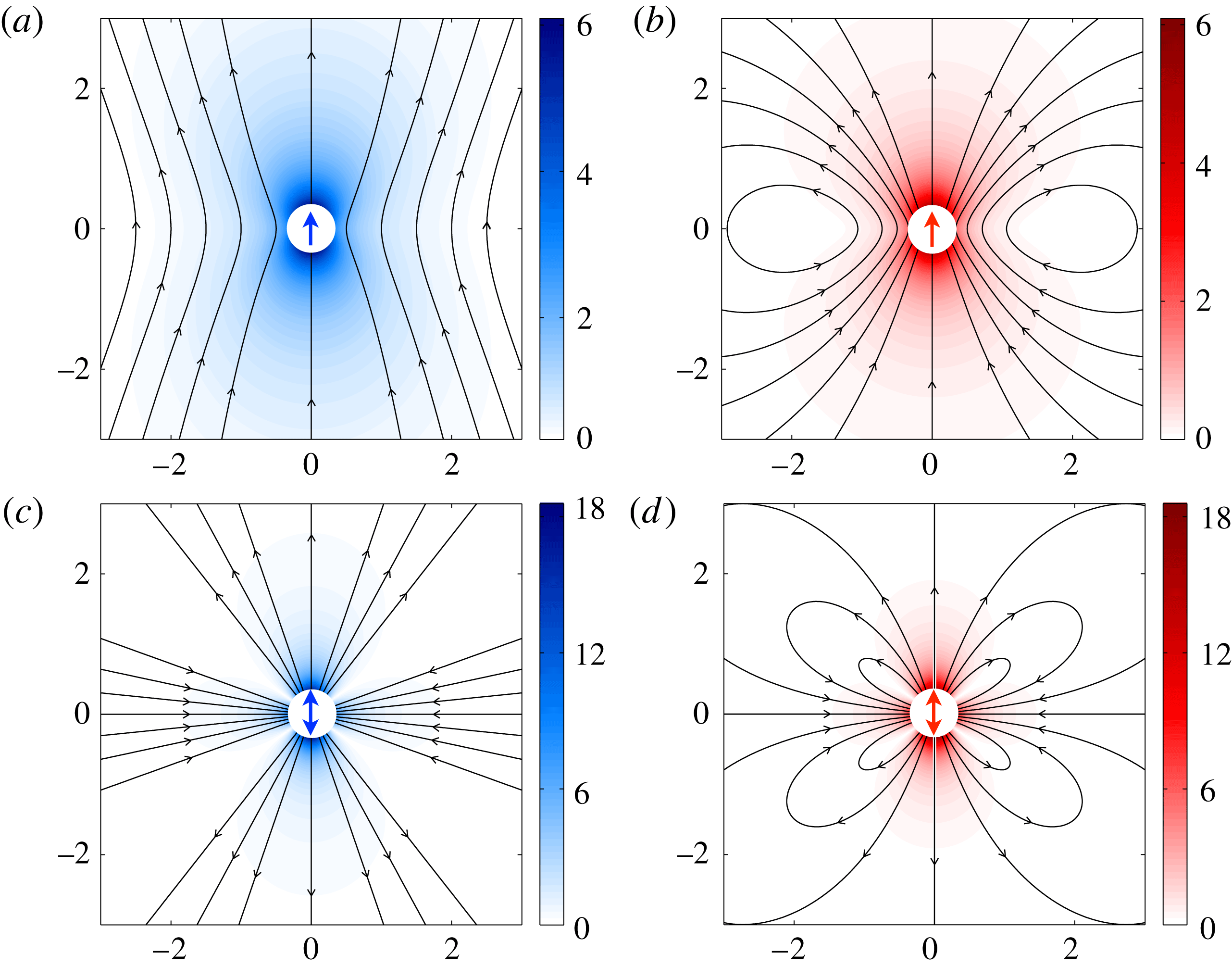
. We contrast the flows generated by a Stokeslet (figure 3
a) and that by a Brinkmanlet (figure 3
b). In a viscous fluid, a Stokeslet
 ${\mathcal{G}}$
decays as
 $1/r$
in the far field, whereas a Brinkmanlet decays much faster as
 $1/r^{3}$
in a porous medium because the velocity disturbance is screened (Koch & Brady Reference Koch and Brady1985; Koch, Hill & Sangani Reference Koch, Hill and Sangani1998; Long & Ajdari Reference Long and Ajdari2001).
4.1.2 Brinkman dipole
A Stokes dipole can be obtained by taking a derivative of a Stokeslet, which corresponds to the flow generated by two point forces in Stokes flows. The specific arrangement of the force dipole can represent different types of swimmers (pushers, pullers, or neutral swimmers; see § 2.2). Similarly, a Brinkman dipole
 ${\mathcal{B}}_{D}$
can be obtained by taking a derivative of a Brinkmanlet (directed in the
 $\unicode[STIX]{x1D736}_{1}$
-direction) along the direction
 $\unicode[STIX]{x1D736}_{2}$
as
 ${\mathcal{B}}_{D}(\unicode[STIX]{x1D736}_{1},\unicode[STIX]{x1D736}_{2})=\unicode[STIX]{x1D736}_{2}\boldsymbol{\cdot }\unicode[STIX]{x1D735}{\mathcal{B}}(\unicode[STIX]{x1D736}_{1})$
. For instance, a Brinkman dipole with
 $\unicode[STIX]{x1D736}_{1}=\unicode[STIX]{x1D736}_{2}=\boldsymbol{e}_{z}$
(the two point forces pointing towards each other) produces the flow
 $$\begin{eqnarray}\displaystyle {\mathcal{B}}_{D}(\boldsymbol{e}_{z},\boldsymbol{e}_{z}) & = & \displaystyle -\frac{[3-\text{e}^{-r\unicode[STIX]{x1D6FF}}(3+3r\unicode[STIX]{x1D6FF}+r^{2}\unicode[STIX]{x1D6FF}^{2})][1+3\cos (2\unicode[STIX]{x1D703})]}{r^{4}\unicode[STIX]{x1D6FF}^{2}}\,\boldsymbol{e}_{r}\nonumber\\ \displaystyle & & \displaystyle -\,\frac{[6-\text{e}^{-r\unicode[STIX]{x1D6FF}}(6+6r\unicode[STIX]{x1D6FF}+3r^{2}\unicode[STIX]{x1D6FF}^{2}+r^{3}\unicode[STIX]{x1D6FF}^{3})]\sin (2\unicode[STIX]{x1D703})}{r^{4}\unicode[STIX]{x1D6FF}^{2}}\,\boldsymbol{e}_{\unicode[STIX]{x1D703}}.\end{eqnarray}$$
We plot in figure 3(c,d) a Stokes dipole and a Brinkman dipole, respectively, for comparison. A Brinkman dipole
 ${\mathcal{B}}_{D}$
decays as
 $1/r^{4}$
in contrast to a Stokes dipole
 ${\mathcal{G}}_{D}$
, which decays as
 $1/r^{2}$
. As a remark, unlike a Stokes dipole
 ${\mathcal{G}}_{D}$
, which generates only radial flows, the Brinkman dipole
 ${\mathcal{B}}_{D}$
generates both radial and tangential flows.
Fundamental singularities in Stokes and Brinkman flows. Streamlines and local speed of the flow due to a point force in (a) Stokes flows (termed a Stokeslet) and (b) Brinkman flows (termed a Brinkmanlet). In (c,d), the flow due to a Stokes force dipole and Brinkman force dipole are shown, respectively. The dimensionless resistance
 $\unicode[STIX]{x1D6FF}=1$
. The colour represents the magnitude of local flow velocity.

4.2 Flow representation by singularities and far-field behaviours
4.2.1 The pumping problem
In the pumping problem, the flow is generated by a squirmer held fixed in space by an external force. We therefore expect the presence of a point force in the decomposition in terms of singularities. Indeed, the flow due to the
 $B_{1}$
mode in the pumping problem (3.6) can be expressed as a combination of Brinkmanlet
 ${\mathcal{B}}$
and source dipole
 ${\mathcal{S}}$
as
 $$\begin{eqnarray}\boldsymbol{u}_{P,B_{1}}=-\frac{\text{e}^{\unicode[STIX]{x1D6FF}}}{2}{\mathcal{B}}+\frac{\text{e}^{\unicode[STIX]{x1D6FF}}-1-\unicode[STIX]{x1D6FF}}{\unicode[STIX]{x1D6FF}^{2}}{\mathcal{S}},\end{eqnarray}$$
where the source dipole
 ${\mathcal{S}}=(2\cos \unicode[STIX]{x1D703}\,\boldsymbol{e}_{r}+\sin \unicode[STIX]{x1D703}\,\boldsymbol{e}_{\unicode[STIX]{x1D703}})/r^{3}$
. We contrast the flow due to the
 $B_{1}$
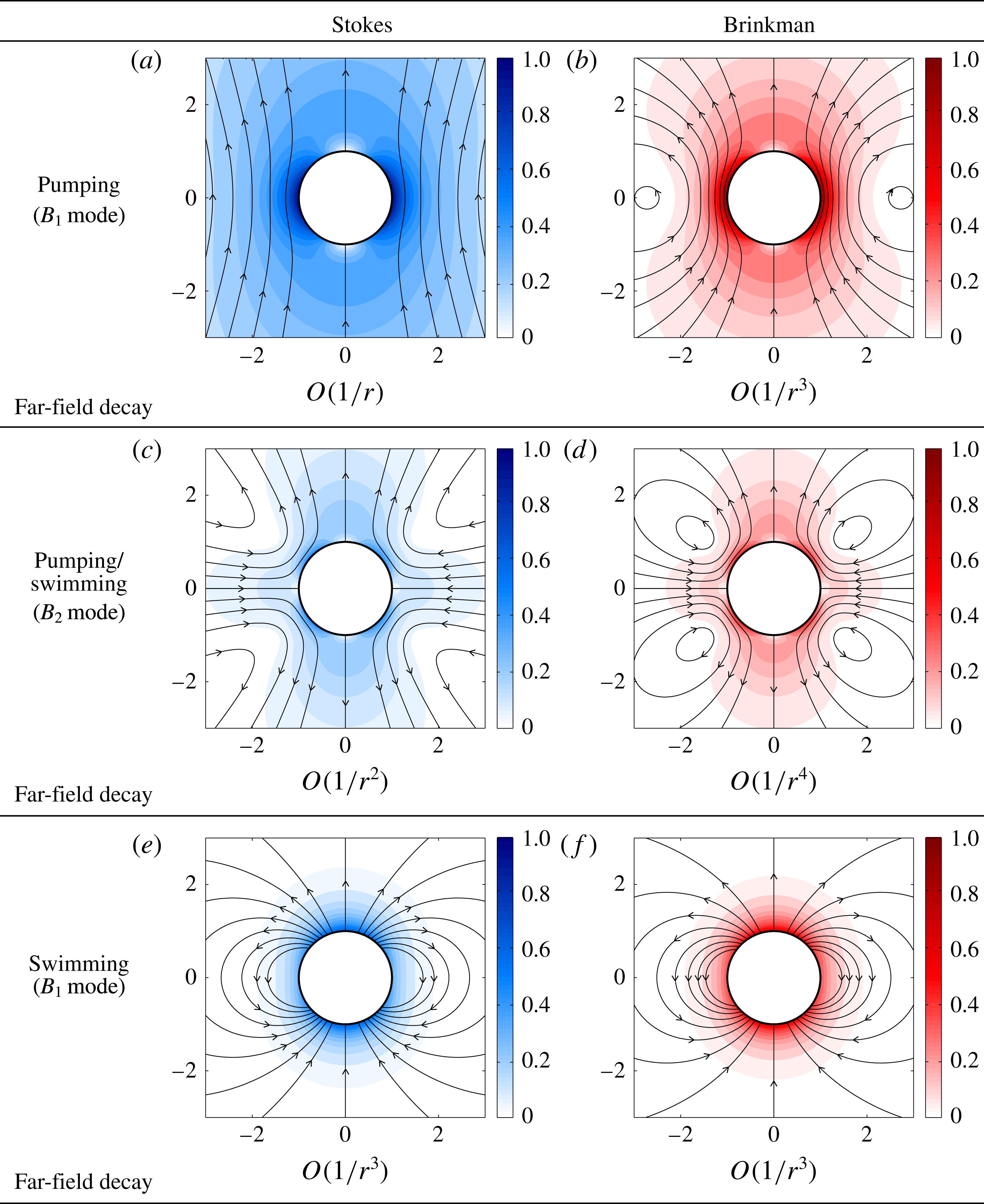
mode in the pumping problem in the Stokes regime (figure 4
a) with that in the Brinkman regime (figure 4
b). In a purely viscous fluid, the far-field behaviour is dominated by a Stokeslet, which decays slowly as
 $1/r$
. In a Brinkman medium, the flow due to the
 $B_{1}$
mode decays rapidly as
 $1/r^{3}$
but the far-field behaviour is not dominated by only the Brinkmanlet; instead, the Brinkmanlet
 ${\mathcal{B}}$
and source dipole
 ${\mathcal{S}}$
both decay as
 $1/r^{3}$
and contribute to the far-field behaviour.
The flow induced by the
 $B_{2}$
mode remains the same in the pumping (3.7) and swimming (3.14) problems, because this mode does not contribute to swimming (Pak & Lauga Reference Pak and Lauga2014; Pedley Reference Pedley2016). The
 $B_{2}$
mode in a Stokes flow represents the action of a force dipole and therefore contains the signature of the propulsion mechanism. Similarly the flow due to the
 $B_{2}$
mode in a Brinkman flow,
 $$\begin{eqnarray}\boldsymbol{u}_{P,B_{2}}=\boldsymbol{u}_{B_{2}}=\frac{\text{e}^{\unicode[STIX]{x1D6FF}}}{2(1+\unicode[STIX]{x1D6FF})}{\mathcal{B}}_{D}+\frac{3\text{e}^{\unicode[STIX]{x1D6FF}}-(3+3\unicode[STIX]{x1D6FF}+\unicode[STIX]{x1D6FF}^{2})}{2\unicode[STIX]{x1D6FF}^{2}(1+\unicode[STIX]{x1D6FF})}{\mathcal{Q}},\end{eqnarray}$$
contains a Brinkman dipole
 ${\mathcal{B}}_{D}$
given by (4.3) plus a source quadrupole
 ${\mathcal{Q}}=\{[1+3\cos (2\unicode[STIX]{x1D703})]\,\boldsymbol{e}_{r}+2\sin (2\unicode[STIX]{x1D703})\,\boldsymbol{e}_{\unicode[STIX]{x1D703}}\}/r^{4}$
. The flow due to the
 $B_{2}$
mode in the Stokes regime (figure 4
c) is compared with that in a Brinkman medium (figure 4
d). In Stokes flows, the force dipole decays as
 $1/r^{2}$
and dominates the source quadrupole in the far field. In contrast, in a Brinkman medium the force dipole and source quadrupole both decay as
 $1/r^{4}$
in the far field.
Streamlines, local speed and far-field decay of the flow around a squirmer in the pumping and swimming problems. Flow around a squirmer with
 $B_{1}$
mode held fixed by an external force in the pumping problem in (a) Stokes and (b) Brinkman flows (
 $B_{1}=1$
,
 $\unicode[STIX]{x1D6FF}=1$
). Panels (c,d) display, respectively, the flow due to the
 $B_{2}$
mode in Stokes and Brinkman flows (
 $B_{2}=-1$
,
 $\unicode[STIX]{x1D6FF}=1$
), which remain the same in pumping and swimming problems because the
 $B_{2}$
mode does not contribute to propulsion. Panels (e,f) show the flow around a self-propelling squirmer with
 $B_{1}$
mode in Stokes and Brinkman flows, respectively (
 $B_{1}=1$
,
 $\unicode[STIX]{x1D6FF}=1$
). The colour represents the magnitude of local flow velocity.

4.2.2 The swimming problem
In Stokes flows, for a squirmer held fixed in space by an external force (the pumping problem), the
 $B_{1}$
mode induces a Stokeslet in the surrounding flow. When the external force is removed, the squirmer with the
 $B_{1}$
mode self-propels at a speed such that the total force acting on the squirmer becomes zero. In terms of flow singularities, one can find that the Stokeslet induced by the translational motion of the squirmer cancels exactly the Stokeslet component in the pumping problem. As a result, the flow surrounding a self-propelling squirmer does not contain any Stokeslets but only a source dipole, which does not contribute a net force and decays as
 $1/r^{3}$
(figure 4
e). For a two-mode squirmer (pusher or puller) in Stokes flows, the force dipole in the
 $B_{2}$
mode decays as
 $1/r^{2}$
and hence dominates the source dipole in the
 $B_{1}$
mode in the far field. These flow characteristics allow far-field models distinguishing pushers and pullers to be effectively constructed in Stokes flows.
However, a self-propelling squirmer has more complex flow structures in a Brinkman medium. Analogous to Stokes flows, the translation of a spherical body induces a Brinkmanlet
 ${\mathcal{B}}$
plus a source dipole
 ${\mathcal{S}}$
. The exact solution in (3.8) can be expressed in terms of singularities in Brinkman flows as
 $\boldsymbol{u}_{T}=U\{3\text{e}^{\unicode[STIX]{x1D6FF}}{\mathcal{B}}/2-[3\text{e}^{\unicode[STIX]{x1D6FF}}-(3+3\unicode[STIX]{x1D6FF}+\unicode[STIX]{x1D6FF}^{2})]{\mathcal{S}}/\unicode[STIX]{x1D6FF}^{2}\}/2$
. However, unlike Stokes flows, the Brinkmanlet and the source dipole both contribute to the net force. When the squirmer is allowed to swim freely, the Brinkmanlet induced by the translational motion thus does not completely cancel the Brinkmanlet component in the pumping problem. Instead, the flow surrounding a self-propelling squirmer, given by (3.13) and (3.14), is represented by a combination of Brinkmanlet and source dipole,
 $$\begin{eqnarray}\boldsymbol{u}_{B_{1}}=-\frac{\unicode[STIX]{x1D6FF}^{2}\text{e}^{\unicode[STIX]{x1D6FF}}}{2(9+9\unicode[STIX]{x1D6FF}+\unicode[STIX]{x1D6FF}^{2})}{\mathcal{B}}+\frac{\text{e}^{\unicode[STIX]{x1D6FF}}+2(1+\unicode[STIX]{x1D6FF})}{9+9\unicode[STIX]{x1D6FF}+\unicode[STIX]{x1D6FF}^{2}}{\mathcal{S}}.\end{eqnarray}$$
Here both the Brinkmanlet and source dipole decay as
 $1/r^{3}$
, contributing to the overall
 $1/r^{3}$
decay in the far field. We remark that, although the flow around a self-propelling squirmer due to the
 $B_{1}$
mode decays as
 $1/r^{3}$
in both Stokes and Brinkman flows (figure 4
e,f), they have different types of constituent singularities. The Stokes flow contains only a source dipole, while the Brinkman flow contains both a Brinkmanlet and a source dipole.
The
 $B_{2}$
mode corresponds to the force dipole exerted on the fluid by the swimmer to generate propulsion. It thus contains information about the propulsion mechanism of different types of swimmers (pushers versus pullers). The additional resistance in porous media has substantial modifications on the far-field behaviours of these two-mode squirmers. In Stokes flows, the
 $B_{2}$
mode dominates the flow in the far field, meaning that the propulsion mechanism of the swimmer determines the character of the far-field flow. However, in Brinkman flows the
 $B_{2}$
mode (decaying as
 $1/r^{4}$
) has a faster spatial decay than the
 $B_{1}$
mode (
 $1/r^{3}$
). This implies that different types of swimmers (pushers versus pullers) then become less distinguishable in the far field in porous media compared with the corresponding Stokes case. These qualitative changes may result in significant differences in hydrodynamic interactions and collective behaviours observed in Stokes flows, especially phenomena critically dependent on the difference in propulsion mechanisms of pushers and pullers (Marchetti et al.
Reference Marchetti, Joanny, Ramaswamy, Liverpool, Prost, Rao and Simha2013; Saintillan & Shelley Reference Saintillan and Shelley2015; Saintillan Reference Saintillan2018).
5 Concluding remarks
In this work, we consider a canonical model swimmer, the squirmer, to study locomotion in heterogeneous viscous media described by the Brinkman equation. The use of an idealized model allows an analytical and exact solution to the Brinkman equation. Our analysis extends the classical results by Lighthill (Reference Lighthill1952) and Blake (Reference Blake1971) in Stokes flows to Brinkman flows. The results enable the calculation of the flow surrounding the squirmer and hence its power dissipation and swimming efficiency, complementing information on propulsion speed previously obtained via the reciprocal theorem (Leshansky Reference Leshansky2009).
Although the propulsion speed of a squirmer with tangential surface velocities decreases monotonically with the additional resistance in a Brinkman medium (Leshansky Reference Leshansky2009), we show that the swimming efficiency can be enhanced relative to the Stokes case. There exists an optimal value of dimensionless resistance maximizing the swimming efficiency. We also examine the structure of the flow surrounding a squirmer in terms of singularities and study the far-field behaviours of squirming in a Brinkman medium. In stark contrast to the Stokes case, our results reveal that the second mode, which contains the signature of the propulsion mechanism, decays faster than the first mode (the swimming mode) in a Brinkman medium. The difference between pushers and pullers thus becomes less distinguishable in the far field of a Brinkman medium. Its consequence on the hydrodynamic interaction and collective behaviours of swimmers observed in Stokes flows presents an interesting subject for future studies. Our results on the flow surrounding a squirmer also enable subsequent analyses on nutrient transport and uptake by micro-organisms in heterogeneous viscous environments (Magar et al. Reference Magar, Goto and Pedley2003; Michelin & Lauga Reference Michelin and Lauga2011). Future work in these directions is currently under way.
Acknowledgements
Helpful correspondence with D. Palaniappan is greatly appreciated. O.S.P. acknowledges support from a Packard Junior Faculty Fellowship.
Appendix A. Squirming with radial surface velocities
Although squirmers with tangential surface velocities are more commonly studied in the literature (Pedley Reference Pedley2016), we also present in this appendix results on squirming with radial surface velocities for completeness. Similar to squirming with tangential surface velocities, the propulsion speed of a squirmer with radial surface velocities in a Brinkman medium can be obtained via the reciprocal theorem without knowing the surrounding flow (Leshansky Reference Leshansky2009). However, the calculation of power dissipation and swimming efficiency relies on knowledge of the surrounding flow. By following similar procedures outlined in § 2, we can readily obtain the associated flow field around the squirmer, which enables the calculations of its power dissipation and swimming efficiency.
A.1 Flow around a self-propelling squirmer with radial surface velocities
Following the formulation by Lighthill (Reference Lighthill1952) and Blake (Reference Blake1971), the radial surface velocities on a squirmer in dimensional form can be expressed as
 $$\begin{eqnarray}\boldsymbol{u}(r=a)=\mathop{\sum }_{n=1}^{\infty }A_{n}P_{n}(\cos \unicode[STIX]{x1D703})\boldsymbol{e}_{r},\end{eqnarray}$$
where
 $A_{n}$
and
 $P_{n}(\cos \unicode[STIX]{x1D703})$
represent a radial mode of surface velocity and a Legendre function, respectively. Following the solution method outlined previously with the boundary condition for radial surface velocity given in (A 1), we can obtain the velocity field around a self-propelling squirmer in the laboratory frame as
 $$\begin{eqnarray}\displaystyle u & = & \displaystyle \frac{[1+\unicode[STIX]{x1D6FF}+\unicode[STIX]{x1D6FF}^{2}-\text{e}^{\unicode[STIX]{x1D6FF}-r\unicode[STIX]{x1D6FF}}(1+r\unicode[STIX]{x1D6FF})]\cos \unicode[STIX]{x1D703}\,A_{1}}{r^{3}\unicode[STIX]{x1D6FF}^{2}}+U\cos \unicode[STIX]{x1D703}\left[\frac{3+3\unicode[STIX]{x1D6FF}+\unicode[STIX]{x1D6FF}^{2}-3\text{e}^{\unicode[STIX]{x1D6FF}-r\unicode[STIX]{x1D6FF}}(1+r\unicode[STIX]{x1D6FF})}{r^{3}\unicode[STIX]{x1D6FF}^{2}}\right]\nonumber\\ \displaystyle & & \displaystyle +\,\mathop{\sum }_{n=2}^{\infty }\frac{-r^{-2-n}A_{n}P_{n}(\cos \unicode[STIX]{x1D703})}{[-\unicode[STIX]{x1D6FF}\text{K}_{n-1/2}(\unicode[STIX]{x1D6FF})+(1+2n)\text{K}_{n+1/2}(\unicode[STIX]{x1D6FF})-\unicode[STIX]{x1D6FF}\text{K}_{n+3/2}(\unicode[STIX]{x1D6FF})]}\nonumber\\ \displaystyle & & \displaystyle \times \,[\unicode[STIX]{x1D6FF}\text{K}_{n-1/2}(\unicode[STIX]{x1D6FF})-\text{K}_{n+1/2}(\unicode[STIX]{x1D6FF})+\unicode[STIX]{x1D6FF}\text{K}_{n+3/2}(\unicode[STIX]{x1D6FF})-2nr^{n+1/2}\text{K}_{n+1/2}(r\unicode[STIX]{x1D6FF})],\end{eqnarray}$$
 $$\begin{eqnarray}\displaystyle v & = & \displaystyle \frac{[1+\unicode[STIX]{x1D6FF}+\unicode[STIX]{x1D6FF}^{2}-\text{e}^{\unicode[STIX]{x1D6FF}-r\unicode[STIX]{x1D6FF}}(1+r\unicode[STIX]{x1D6FF}+r^{2}\unicode[STIX]{x1D6FF}^{2})]\sin \unicode[STIX]{x1D703}\,A_{1}}{2r^{3}\unicode[STIX]{x1D6FF}^{2}}\nonumber\\ \displaystyle & & \displaystyle +\,U\sin \unicode[STIX]{x1D703}\left[\frac{3+3\unicode[STIX]{x1D6FF}+\unicode[STIX]{x1D6FF}^{2}-3\text{e}^{\unicode[STIX]{x1D6FF}-r\unicode[STIX]{x1D6FF}}(1+r\unicode[STIX]{x1D6FF}+r^{2}\unicode[STIX]{x1D6FF}^{2})}{2r^{3}\unicode[STIX]{x1D6FF}^{2}}\right]\nonumber\\ \displaystyle & & \displaystyle +\,\mathop{\sum }_{n=2}^{\infty }\frac{nr^{-2-n}A_{n}V_{n}(\cos \unicode[STIX]{x1D703})}{2[-\unicode[STIX]{x1D6FF}\text{K}_{n-1/2}(\unicode[STIX]{x1D6FF})+(1+2n)\text{K}_{n+1/2}(\unicode[STIX]{x1D6FF})-\unicode[STIX]{x1D6FF}\text{K}_{n+3/2}(\unicode[STIX]{x1D6FF})]}\nonumber\\ \displaystyle & & \displaystyle \times \,[\!-\unicode[STIX]{x1D6FF}\text{K}_{n-1/2}(\unicode[STIX]{x1D6FF})+\text{K}_{n+1/2}(\unicode[STIX]{x1D6FF})\nonumber\\ \displaystyle & & \displaystyle -\,\unicode[STIX]{x1D6FF}\text{K}_{n+3/2}(\unicode[STIX]{x1D6FF})+\unicode[STIX]{x1D6FF}r^{n+3/2}\text{K}_{n-1/2}(r\unicode[STIX]{x1D6FF})-r^{n+1/2}\text{K}_{n+1/2}(r\unicode[STIX]{x1D6FF})+\unicode[STIX]{x1D6FF}r^{n+3/2}\text{K}_{n+3/2}(r\unicode[STIX]{x1D6FF})\!],\nonumber\\ \displaystyle & & \displaystyle\end{eqnarray}$$
where
 $U$
is the unknown swimming speed due to radial surface velocities.
We use the above flow field and enforce the force-free condition (3.9) to obtain the unknown swimming speed as
 $$\begin{eqnarray}U=-\frac{3+3\unicode[STIX]{x1D6FF}+\unicode[STIX]{x1D6FF}^{2}}{9+9\unicode[STIX]{x1D6FF}+\unicode[STIX]{x1D6FF}^{2}}A_{1},\end{eqnarray}$$
which agrees with the results obtained via the reciprocal theorem by Leshansky (Reference Leshansky2009). Similar to squirming in Stokes flows, only the
 $A_{1}$
mode contributes to propulsion. In the limit
 $\unicode[STIX]{x1D6FF}\rightarrow 0$
, the propulsion speed reduces to
 $-A_{1}/3$
in the Stokes case (Lighthill Reference Lighthill1952; Blake Reference Blake1971). As the resistance
 $\unicode[STIX]{x1D6FF}$
increases, the propulsion speed increases monotonically, in contrast to the case of squirming with tangential surface velocities, where a monotonic decrease in speed is observed.
A.2 Power dissipation and swimming efficiency
With the knowledge of the flow field, the power dissipation
 ${\mathcal{P}}$
and swimming efficiency
 $\unicode[STIX]{x1D702}$
can be calculated. For instance, the power dissipation and swimming efficiency associated with the swimming motion due to the
 $A_{1}$
mode are given by
 $$\begin{eqnarray}{\mathcal{P}}=\frac{40\unicode[STIX]{x03C0}(18+18\unicode[STIX]{x1D6FF}+3\unicode[STIX]{x1D6FF}^{2}+\unicode[STIX]{x1D6FF}^{3})(1+\unicode[STIX]{x1D6FF})\unicode[STIX]{x1D707}aA_{1}^{2}}{15(1+\unicode[STIX]{x1D6FF})(9+9\unicode[STIX]{x1D6FF}+\unicode[STIX]{x1D6FF}^{2})}\end{eqnarray}$$
and
 $$\begin{eqnarray}\unicode[STIX]{x1D702}=\frac{5(1+\unicode[STIX]{x1D6FF})(3+3\unicode[STIX]{x1D6FF}+\unicode[STIX]{x1D6FF}^{2})^{2}}{20(18+18\unicode[STIX]{x1D6FF}+3\unicode[STIX]{x1D6FF}^{2}+\unicode[STIX]{x1D6FF}^{3})(1+\unicode[STIX]{x1D6FF})},\end{eqnarray}$$
respectively. As expected, we recover the Stokes power dissipation (
 $P_{S}=16\unicode[STIX]{x03C0}\unicode[STIX]{x1D707}aA_{1}^{2}/3$
) and swimming efficiency
 $(\unicode[STIX]{x1D702}_{S}=1/8)$
in the limit
 $\unicode[STIX]{x1D6FF}\rightarrow 0$
(Blake Reference Blake1971). The expressions for other modes can be obtained in the same manner. Unlike squirming with tangential surface velocities, in which case an optimal resistance
 $\unicode[STIX]{x1D6FF}$
maximizing the swimming efficiency exists, the swimming efficiency for the radial case increases monotonically with
 $\unicode[STIX]{x1D6FF}$
. To summarize, both swimming speed and efficiency are enhanced in the case of squirming with radial surface velocities in a Brinkman medium.