1. Introduction
Turbulent multiphase flows are important to a large variety of applications such as spray combustion, material processing, spray coating, etc. All three computational strategies, namely direct numerical simulation (DNS), large-eddy simulation (LES), and Reynolds-averaged simulation (RAS), have been employed for the analysis of multiphase turbulent flows with and without chemical reaction. In a review article, Mashayek & Pandya (Reference Mashayek and Pandya2003) provide a comprehensive collection of the DNS studies of multiphase flows by categorizing them based on flow configuration and coupling between the phases. Homogeneous two-phase turbulent flows have been the subject of a large number of these DNS studies (Squires & Eaton Reference Squires and Eaton1990a ,Reference Squires and Eaton b , Reference Squires and Eaton1991; Elghobashi & Truesdell Reference Elghobashi and Truesdell1992, Reference Elghobashi and Truesdell1993; Wang & Maxey Reference Wang and Maxey1993; Truesdell & Elghobashi Reference Truesdell and Elghobashi1994; Mashayek et al. Reference Mashayek, Jaberi, Miller and Givi1997; Maxey et al. Reference Maxey, Patel, Chang and Wang1997; Mashayek Reference Mashayek1998a ; Mashayek & Jaberi Reference Mashayek and Jaberi1999; Jaberi & Mashayek Reference Jaberi and Mashayek2000) due to their relative simplicity. Relatively simple inhomogeneous two-phase turbulent flows have also been considered (McLaughlin Reference McLaughlin1989; Brooke et al. Reference Brooke, Kontomaris, Hanratty and McLaughlin1992; Pedinotti, Mariotti & Banerjee Reference Pedinotti, Mariotti and Banerjee1992; Ounis, Ahmadi & McLaughlin Reference Ounis, Ahmadi and McLaughlin1993; Brooke, Hanratty & McLaughlin Reference Brooke, Hanratty and McLaughlin1994; Miller & Bellan Reference Miller and Bellan1994; Chen & McLaughlin Reference Chen and McLaughlin1995; Mashayek Reference Mashayek1998a ,Reference Mashayek b ; Ling, Chung & Crowe Reference Ling, Chung and Crowe2000; Menon Reference Menon, Friedrich and Rodi2000; Okong’o & Bellan Reference Okong’o and Bellan2000; Liao, Mashayek & Guo Reference Liao, Mashayek and Guo2001; Almeida & Jaberi Reference Almeida and Jaberi2006, Reference Almeida and Jaberi2008; Kuerten Reference Kuerten2006). This is partly due to limitations of DNS but in no way implies a shortcoming of the method. On the contrary, DNS has proved to be very effective in capturing many physical phenomena which could not have been studied by any other means. It has also been very useful in assessing the performances of many of the closures in RAS and LES. RAS has been the method of choice for practical applications and this trend will continue for many years to come. This is the case even with proven non-universality of the currently employed RAS closures for multiphase turbulent (non)-reacting flows. It can be argued that LES provides the optimum means of capturing the unsteady physical features of complex turbulent flows, such as multiphase reacting flows. For this reason, LES has experienced significant growth in the past few decades and has been widely applied to multiphase flows. However, the predictive capability of LES remains dependent on the success of its subgrid-scale (SGS) closures as well as the numerical method used for the solution of LES equations.
The numerical methods that have been developed for multiphase flows are generally based on three different approaches: (i) the Eulerian–Eulerian approach (Scardovelli & Zaleski Reference Scardovelli and Zaleski1999; Shyy & Narayanan Reference Shyy and Narayanan1999; Lakehal Reference Lakehal2002; Pandya & Mashayek Reference Pandya and Mashayek2002; Herrmann Reference Herrmann2003; Mashayek & Pandya Reference Mashayek and Pandya2003; Sethian & Smereka Reference Sethian and Smereka2003; Cuenot et al. Reference Cuenot, Boileau, Pascaud, Mossa, Riber, Poinsot and B’erat2006), (ii) the Eulerian–Lagrangian approach (Faeth Reference Faeth1987; Shirolkar, Coimbra & McQuay Reference Shirolkar, Coimbra and McQuay1996; Crowe, Sommerfeld & Tsuji Reference Crowe, Sommerfeld and Tsuji1998; Sirignano Reference Sirignano1999; Bellan Reference Bellan2000; Loth Reference Loth2000; Apte, Gorokhovski & Moin Reference Apte, Gorokhovski and Moin2003; Mashayek & Pandya Reference Mashayek and Pandya2003; Mahesh et al. Reference Mahesh, Constantinescu, Apte, Iaccarino, Ham and Moin2006; Menon & Patel Reference Menon and Patel2006; Patel et al. Reference Patel, Kirtas, Sankaran and Menon2007), and (iii) the Lagrangian–Lagrangian approach (Salman & Soteriou Reference Salman and Soteriou2004; Seta, Kono & Chen Reference Seta, Kono and Chen2003; Chen & Doolen Reference Chen and Doolen1998). In the first approach, the continuum transport equations for both phases are solved. These equations are somewhat similar and are often obtained by some sort of volume averaging, which is conceptually different to the ensemble averaging in RAS or space averaging in LES. In the second approach, the continuum carrier fluid equations are solved in their instantaneous form in DNS or in averaged form in RAS and LES over a fixed Eulerian grid system. However, the second phase is described by a set of modelled Lagrangian equations which determine the position, velocity, temperature, and other properties (Crowe et al. Reference Crowe, Sommerfeld and Tsuji1998; Sirignano Reference Sirignano1999; Loth Reference Loth2000; Mashayek & Pandya Reference Mashayek and Pandya2003) of the dispersed phase. In the third method, both phases are described in the Lagrangian context. The Eulerian–Eulerian and Eulerian–Lagrangian models have been employed for RAS, LES and DNS of a wide range of two-phase or two-fluid turbulent flows including free surface flows, or particle-laden turbulent flows (Faeth Reference Faeth1987; Shirolkar et al. Reference Shirolkar, Coimbra and McQuay1996; Crowe et al. Reference Crowe, Sommerfeld and Tsuji1998; Scardovelli & Zaleski Reference Scardovelli and Zaleski1999; Shyy & Narayanan Reference Shyy and Narayanan1999; Sirignano Reference Sirignano1999; Bellan Reference Bellan2000; Loth Reference Loth2000; Menon Reference Menon, Friedrich and Rodi2000; Lakehal Reference Lakehal2002; Mashayek & Pandya Reference Mashayek and Pandya2003; Sethian & Smereka Reference Sethian and Smereka2003; Cressman et al. Reference Cressman, Davoudi, Goldburg and Schumacher2004; Moin Reference Moin2004; Madnia, Jaberi & Givi Reference Madnia, Jaberi, Givi, Minkowycz, Sparrow and Murthy2006). In comparison, there is a limited number of models based on the Lagrangian–Lagrangian approach. Examples are the two-phase random vortex model (Salman & Soteriou Reference Salman and Soteriou2004) and the two-phase Lattice Boltzmann model (Chen & Doolen Reference Chen and Doolen1998; Seta et al. Reference Seta, Kono and Chen2003).
Multiphase flow systems are often divided into various regimes: dilute, moderately dense, and very dense. All of these regimes are present in sprays (Dukowicz 1980; Faeth Reference Faeth1983, Reference Faeth1987; Lefebvre Reference Lefebvre1989; Ashgriz & Poo Reference Ashgriz and Poo1991; Yeh & Lei Reference Yeh and Lei1991a ,Reference Yeh and Lei b ; Crowe et al. Reference Crowe, Sommerfeld and Tsuji1998; Lin & Reitz Reference Lin and Reitz1998; Armenio, Piomelli & Fiorotto Reference Armenio, Piomelli and Fiorotto1999; Sirignano Reference Sirignano1999; Boivin, Simonin & Squires Reference Boivin, Simonin and Squires2000; Lasheras & Hopfinger Reference Lasheras and Hopfinger2000; Schmidt & Rutland Reference Schmidt and Rutland2000; Shen & Yue Reference Shen and Yue2001; Yamamoto et al. Reference Yamamoto, Potthoff, Tanaka, Kajishima and Tsuji2001; Yuu, Ueno & Umekage Reference Yuu, Ueno and Umekage2001; Post & Abraham Reference Post and Abraham2002; Sankaran & Menon Reference Sankaran and Menon2002; Apte et al. Reference Apte, Mahesh, Moin and Oefelein2003; Okong’o & Bellan Reference Okong’o and Bellan2004; Leboissetier, Okong’o & Bellan Reference Leboissetier, Okong’o and Bellan2005; Li, Jaberi & Shih Reference Li, Jaberi and Shih2007). In the dilute flow regime, particle–particle interactions are rare and the volume fraction of the particle to carrier fluid is very small, making the continuum assumption and Eulerian–Eulerian formulation essentially invalid. In these regimes, the particles are often treated as point masses which are affected by the carrier gas through mass, momentum, and energy interactions. The coupling could be two-way, allowing the particles to modify the carrier fluid as well.
The Eulerian–Lagrangian dilute two-phase LES models have been applied to various turbulent flows in complex geometries. For example, Apte et al. (Reference Apte, Mahesh, Moin and Oefelein2003) considered solid particle dispersion in a non-reacting swirling coaxial jet combustor. In this work, the incompressible Eulerian carrier fluid equations are solved with an unstructured grid and the cell-averaged effects of particles on the turbulence are incorporated through a source term in the momentum equation. Also in this work, as in others mentioned above, a modified (nonlinear) version of the Stokes equation is used for the particle transport (Crowe et al. Reference Crowe, Sommerfeld and Tsuji1998; Sirignano Reference Sirignano1999; Loth Reference Loth2000). By comparing their numerical results with the experimental data, Apte et al. (Reference Apte, Mahesh, Moin and Oefelein2003) indicated that the LES predictions are significantly more accurate than those of RAS, despite the fact that the effects of SGS fluctuations of the carrier fluid on the particles are ignored in their LES calculations. Consistently, by comparing various multiphase turbulent flow models for environmental and hydrodynamic applications, Lakehal (Reference Lakehal2002) concluded that RAS models are inherently inadequate for these applications and should be transcended by LES models.
The particle tracking LES models discussed above are based on point mass (or point volume) approximations which are only suitable for dilute systems with insignificant particle to carrier fluid volume fraction. In theory, it is possible to simulate the flow domain outside the particle in the boundary layer and wake region. However, these simulations, referred to as resolved-volume simulations, are very expensive and usually limited to one or a handful of particles in simple flows, and do not seem at present to be practical for LES. Also, as discussed below, Eulerian–Eulerian mathematical/computational models may be used for dense two-phase flow simulations. However, these models may not be viable for complex turbulent flows that involve preferential concentration of the particles and the simultaneous presence of both dense and dilute regimes. For LES of moderately dense two-phase particulate flows, efficient particle–particle or droplet–droplet collision models are available (Schmidt & Rutland Reference Schmidt and Rutland2000; Post & Abraham Reference Post and Abraham2002), which can be – and have been – incorporated in the Lagrangian particle simulations. For example, by using a Monte Carlo model for the inter-particle collision, Yamamoto et al. (Reference Yamamoto, Potthoff, Tanaka, Kajishima and Tsuji2001) have simulated a gas-particle turbulent flow in a vertical channel, and have shown that by adding the particle–particle collision models, the LES results compare better with those of experiment. More recently, the LES models have been extended and applied to realistic combustion systems (Sankaran & Menon Reference Sankaran and Menon2002; Okong’o & Bellan Reference Okong’o and Bellan2004; Leboissetier et al. Reference Leboissetier, Okong’o and Bellan2005; Mahesh et al. Reference Mahesh, Constantinescu, Apte, Iaccarino, Ham and Moin2006; Patel et al. Reference Patel, Kirtas, Sankaran and Menon2007).
The filtered density function (FDF) and filtered mass density function (FMDF) models (Pope Reference Pope1990; Gao & O’Brien Reference Gao and O’Brien1993; Colucci et al. Reference Colucci, Jaberi, Givi and Pope1998; Jaberi et al. Reference Jaberi, Colucci, James, Givi and Pope1999; Fox Reference Fox2003; Givi Reference Givi2006; Haworth Reference Haworth2010) are considered to be among the most promising models for LES of turbulent reacting flows. In these models, the joint statistics of turbulent variables are obtained by solving the transport equation for the single-point, joint SGS probability density function (PDF) of these variables. One of the important advantages of FMDF is that the single-point quantities such as reaction terms appear in a closed form in its equation. The other advantage is that higher-order statistical information is naturally available from the model. However, the single-point FMDF equations are not completely closed, and some form of modelling for multi-point correlations is needed. Jaberi et al. (Reference Jaberi, Colucci, James, Givi and Pope1999) developed a consistent mathematical formulation and efficient numerical method for the scalar FMDF, which is the SGS PDF of energy and species mass fractions. FDF/FMDF models for velocity (Gicquel et al. Reference Gicquel, Givi, Jaberi and Pope2002), velocity–scalar (Sheikhi et al. Reference Sheikhi, Drozda, Givi and Pope2003; Sheikhi, Givi & Pope Reference Sheikhi, Givi and Pope2007; Nik et al. Reference Nik, Yilmaz, Sheikhi, Givi and Pope2010a ,Reference Nik, Yilmaz, Sheikhi and Givi b ), and frequency–velocity–scalar FMDF (Sheikhi, Givi & Pope Reference Sheikhi, Givi and Pope2009) have also been developed. As mentioned above, in the scalar FMDF transport equation, all chemical source or sink terms are closed, making the model very attractive for simulations of various types of reactions (slow, fast, non-premixed, premixed, etc.) with complex kinetics. Several applications of scalar FMDF to turbulent reacting flows have been reported in the literature (James & Jaberi Reference James and Jaberi2000; Raman, Pitsch & Fox Reference Raman, Pitsch and Fox2005; Sheikhi et al. Reference Sheikhi, Drozda, Givi, Jaberi and Pope2005; Afshari, Jaberi & Shih Reference Afshari, Jaberi and Shih2008; Yaldizli, Mehravaran & Jaberi Reference Yaldizli, Mehravaran and Jaberi2010; Yilmaz et al. Reference Yilmaz, Nik, Givi and Strakey2010). The model has recently been extended to high-speed flows by Banaeizadeh, Li & Jaberi (Reference Banaeizadeh, Li and Jaberi2011). In this study, we discuss the extension of FMDF to two-phase turbulent flows.
The RANS/PDF models have also been extended and used for numerical simulations of multiphase flows involving liquid fuel sprays (Zhu et al. Reference Zhu, Bray, Rumberg and Rogg2000; Minier & Peirano Reference Minier and Peirano2001; Ge & Gutheil Reference Ge and Gutheil2008) and solid dispersed particles (Stollinger et al. Reference Stollinger, Naud, Roekaerts and Heinz2013; Zhao & Haworth Reference Zhao and Haworth2014). In these models, the gas-phase RANS equations are closed with standard turbulence submodels and the assumed PDF or modelled PDF transport equation are solved for the reactive species and temperature fields in the gas phase. Despite the similarities between RANS/PDF and LES/FMDF methods, they are still different in theory and in practice. For example, the FMDF transport equation is derived from the unfiltered DNS equations by applying spatial filtering, as is normally done in LES methods, while the PDF and RANS equations are based on some form of ensemble or time averaging. Also, the three-component numerical methods and submodels used here for the solution of LES/FMDF/droplet equations are different to those used in RANS/PDF methods. Understandably, the success of any multi-component method such as RANS/PDF and LES/FMDF is dependent on the accuracy of its submodels and also the original methodology on which they are based. By comparing various multiphase turbulent flow models, Lakehal (Reference Lakehal2002) and Apte et al. (Reference Apte, Gorokhovski and Moin2003) concluded that the RANS-based models are inadequate for multiphase flow simulations and should be transcended by LES models. The FMDF is a transported PDF model developed for LES, which is extended and applied in this study to multiphase flows.
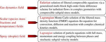
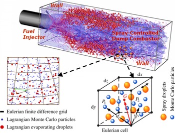
The new two-phase LES/FMDF model is based on an Eulerian–Lagrangian–Lagrangian mathematical/numerical methodology which can handle the two-way interactions between particle and fluid phases for low particle to fluid volume fraction ratios. Figure 1 shows various elements of the model and its computational flow solver in a block diagram. The gas-phase part is solved by a high-order compact finite difference numerical scheme. The subgrid combustion is modelled with the two-phase scalar FMDF and its Lagrangian Monte Carlo numerical method. The liquid/droplet field is simulated with a non-equilibrium Lagrangian model and stochastic SGS closures. The two-way mass, momentum, and energy coupling between phases is implemented through a series of source/sink terms. The LES/FMDF can be implemented with complex multi-step chemistry models for non-equilibrium flames. Finite-rate chemistry effects are explicitly and exactly included in this procedure since the chemistry is closed in the formulation. The LES/FMDF can also be employed in conjunction with equilibrium fuel-oxidation models. These models are enacted via flamelet simulations which normally consider a laminar counterflow (opposed jet) flame configuration. For the two-phase flow calculations presented in this paper, a one-step global non-equilibrium model is used. Details of the two-phase LES/FMDF model are presented in §§ 2 and 3. The results obtained with the model for three different flows, all with spray, droplet evaporation and combustion, are discussed in § 4. Figure 3 shows, for example, the vorticity and mass fraction contours and droplet distribution in one of the simulated flows. In this flow, a lean premixed preheated air–decane flame is controlled by injection of a relatively small amount of liquid
 $n$
-decane fuel. Also shown in this figure are the Eulerian grid points, Lagrangian spray droplets and FMDF Monte Carlo particles. The LES/FMDF results are validated by comparison with DNS data for spatially developing droplet-laden mixing layers. Applicability of the model to more complex problems is demonstrated by considering flow, spray and combustion simulations in a double-swirl spray burner as well as the spray-controlled dump combustor.
A block diagram showing different components of the two-phase LES/FMDF and its Eulerian–Lagrangian–Lagrangian flow solver.

2. Mathematical formulation
The two-phase LES/FMDF model has three main mathematical components: (i) the filtered gas velocity equations, (ii) the FMDF and its equivalent stochastic differential equations for the scalar (gas energy and species mass fractions), (iii) the Lagrangian droplet equations for the liquid phase. These equations are presented in the following sections.
2.1. Carrier gas equations
For a two-phase reacting flow, the conservation equations for mass, momentum, energy and chemical species mass fractions, along with the equation of state, may be written as
 $$\begin{eqnarray}\displaystyle & \displaystyle \frac{\partial {\it\rho}}{\partial t}+\frac{\partial {\it\rho}u_{i}}{\partial x_{i}}=S_{{\it\rho}}, & \displaystyle\end{eqnarray}$$
 $$\begin{eqnarray}\displaystyle & \displaystyle \frac{\partial {\it\rho}u_{j}}{\partial t}+\frac{\partial {\it\rho}u_{i}u_{j}}{\partial x_{i}}=-\frac{\partial p}{\partial x_{j}}+\frac{\partial {\it\tau}_{ij}}{\partial x_{i}}+S_{uj}, & \displaystyle\end{eqnarray}$$
 $$\begin{eqnarray}\displaystyle & \displaystyle \frac{\partial {\it\rho}{\it\phi}_{{\it\alpha}}}{\partial t}+\frac{\partial {\it\rho}u_{i}{\it\phi}_{{\it\alpha}}}{\partial x_{i}}=-\frac{\partial J_{i}^{{\it\alpha}}}{\partial x_{i}}+S_{R}^{{\it\alpha}}+S_{S}^{{\it\alpha}},\quad {\it\alpha}=1,\dots ,N_{s+1}, & \displaystyle\end{eqnarray}$$
 $$\begin{eqnarray}\displaystyle & \displaystyle p={\it\rho}R^{0}T\mathop{\sum }\limits_{{\it\alpha}=1}^{N_{s}}\frac{Y_{{\it\alpha}}}{W_{{\it\alpha}}}, & \displaystyle\end{eqnarray}$$
 ${\it\rho}$
,
 $u_{i}$
,
 $p$
and
 $T$
are the carrier gas density, velocity, pressure and temperature, respectively. For
 ${\it\alpha}=1,2,\dots ,N_{s}$
, the scalars
 ${\it\phi}_{{\it\alpha}}$
represent the species’ mass fractions
 $(Y_{{\it\alpha}})$
, with
 $S_{R}^{{\it\alpha}}$
being the species production or consumption rate due to reaction and
 $S_{S}^{{\it\alpha}}=S_{{\it\rho}}{\it\delta}_{1{\it\alpha}}$
denoting the added mass due to liquid droplet evaporation. For
 ${\it\alpha}=N_{s+1}$
,
 ${\it\phi}_{{\it\alpha}}$
denotes the enthalpy, with
 $S_{R}^{{\it\alpha}}$
being the heat of combustion and
 $S_{S}^{{\it\alpha}}=S_{h}$
representing the droplet effects on the gas energy or enthalpy. The derivation of (2.3) along with the definitions of
 $S_{R}^{{\it\alpha}}$
and
 $S_{S}^{{\it\alpha}}$
are given in appendix A, which indicates that the chemical reaction terms
 $S_{R}^{{\it\alpha}}=S_{R}^{{\it\alpha}}({\it\phi}_{1},{\it\phi}_{2},\dots ,{\it\phi}_{N_{s+1}})$
are only functions of scalars. In (2.4),
 $R^{0}$
and
 $W_{{\it\alpha}}$
are the universal gas constant and species molecular weights, respectively. The viscous stress tensor,
 ${\it\tau}_{ij}$
, and mass and heat flux vectors,
 $J_{i}^{{\it\alpha}}$
, are modelled as
 $$\begin{eqnarray}\displaystyle & \displaystyle {\it\tau}_{ij}={\it\mu}\left(\frac{\partial u_{i}}{\partial x_{j}}+\frac{\partial u_{j}}{\partial x_{i}}-\frac{2}{3}\frac{\partial u_{k}}{\partial x_{k}}{\it\delta}_{ij}\right), & \displaystyle\end{eqnarray}$$
 $$\begin{eqnarray}\displaystyle & \displaystyle J_{i}^{{\it\alpha}}=-{\it\gamma}\frac{\partial {\it\phi}_{{\it\alpha}}}{\partial x_{i}}, & \displaystyle\end{eqnarray}$$
 ${\it\mu}$
is the molecular viscosity and
 ${\it\gamma}={\it\rho}{\it\Gamma}$
is the diffusivity coefficient. The Lewis number is assumed to be unity.
In the hybrid LES/FMDF model, the resolved carrier gas field is obtained by solving the filtered continuity, momentum and energy equations together with the equation of state as shown below. There is no need to solve the filtered scalar equations, as the scalars (gas energy and species mass fractions) are obtained from the FMDF. However, to demonstrate the consistency and reliability of the FMDF and its numerical solution method, the filtered scalar equation is solved here together with other carrier gas equations:
 $$\begin{eqnarray}\displaystyle & \displaystyle \frac{\partial \langle {\it\rho}\rangle _{l}}{\partial t}+\frac{\partial \langle {\it\rho}\rangle _{l}\langle u_{i}\rangle _{L}}{\partial x_{i}}=\langle S_{{\it\rho}}\rangle _{l}, & \displaystyle\end{eqnarray}$$
 $$\begin{eqnarray}\displaystyle & \displaystyle \frac{\partial \langle {\it\rho}\rangle _{l}\langle u_{i}\rangle _{L}}{\partial t}+\frac{\partial \langle {\it\rho}\rangle _{l}\langle u_{i}\rangle _{L}\langle u_{j}\rangle _{L}}{\partial x_{j}}=-\frac{\partial \langle p\rangle _{l}}{\partial x_{i}}+\frac{\partial \langle {\it\tau}_{ij}\rangle _{l}}{\partial x_{i}}-\frac{\partial \unicode[STIX]{x1D61B}_{ij}}{\partial x_{j}}+\langle S_{u_{i}}\rangle _{l}, & \displaystyle\end{eqnarray}$$
 $$\begin{eqnarray}\displaystyle & \displaystyle \frac{\partial \langle {\it\rho}\rangle _{l}\langle {\it\phi}_{{\it\alpha}}\rangle _{L}}{\partial t}+\frac{\partial \langle {\it\rho}\rangle _{l}\langle u_{i}\rangle _{L}\langle {\it\phi}_{{\it\alpha}}\rangle _{L}}{\partial x_{i}}=-\frac{\partial \langle J_{i}^{{\it\alpha}}\rangle _{l}}{\partial x_{i}}-\frac{\partial M_{i}^{{\it\alpha}}}{\partial x_{i}}+\langle S_{R}^{{\it\alpha}}\rangle _{l}+\langle S_{S}^{{\it\alpha}}\rangle _{l},\quad & \displaystyle \nonumber\\ \displaystyle & \displaystyle {\it\alpha}=1,\dots ,N_{s+1}, & \displaystyle\end{eqnarray}$$
 $\langle \,f(\boldsymbol{x},t)\rangle _{l}$
and
 $\langle \,f(\boldsymbol{x},t)\rangle _{L}=\langle {\it\rho}f\rangle _{l}/\langle {\it\rho}\rangle _{l}$
represent the filtered and Favre-filtered values of the transport variable
 $f(\boldsymbol{x},t)$
.
The unclosed terms in the above equations include the SGS stresses,
 $\unicode[STIX]{x1D61B}_{ij}=\langle {\it\rho}\rangle _{l}[\langle u_{i}u_{j}\rangle _{L}-\langle u_{i}\rangle _{L}\langle u_{j}\rangle _{L}]$
, and the SGS energy and scalar fluxes,
 $M_{i}^{{\it\alpha}}=\langle {\it\rho}\rangle _{l}[\langle u_{i}{\it\phi}_{{\it\alpha}}\rangle _{L}-\langle u_{i}\rangle _{L}\langle {\it\phi}_{{\it\alpha}}\rangle _{L}]$
. In multiphase reacting flows, additional models are required for the filtered reaction term
 $\langle S_{R}^{{\it\alpha}}\rangle _{L}$
and the liquid (droplet) term
 $\langle S_{S}^{{\it\alpha}}\rangle _{L}$
, which is the subject of probability formulation described in the next section. For the SGS stress
 $\unicode[STIX]{x1D61B}_{ij}$
and SGS scalar flux
 $M_{i}^{{\it\alpha}}$
, we use the following dynamic gradient type closures:
 $$\begin{eqnarray}\displaystyle & \unicode[STIX]{x1D61B}_{ij}=-2\langle {\it\rho}\rangle _{l}{\it\nu}_{t}\left[\langle \unicode[STIX]{x1D61A}_{ij}\rangle _{L}-\langle \unicode[STIX]{x1D61A}_{kk}\rangle _{L}{\it\delta}_{ij}/3\right]+{\textstyle \frac{2}{3}}\langle {\it\rho}\rangle _{l}K_{SGS}{\it\delta}_{ij}, & \displaystyle\end{eqnarray}$$
 $$\begin{eqnarray}\displaystyle & \displaystyle M_{i}^{{\it\alpha}}=-{\it\gamma}_{t}\frac{\partial \langle {\it\phi}_{{\it\alpha}}\rangle _{L}}{\partial x_{i}}, & \displaystyle\end{eqnarray}$$
 $\langle \unicode[STIX]{x1D61A}_{ij}\rangle _{L}=(\partial \langle u_{i}\rangle _{L}/\partial x_{j}+\partial \langle u_{j}\rangle _{L}/\partial x_{i})/2$
is the resolved strain rate tensor. In (2.11),
 ${\it\gamma}_{t}=\langle {\it\rho}\rangle _{l}{\it\Gamma}_{t}=\langle {\it\rho}\rangle _{l}{\it\nu}_{t}/Sc_{t}$
and
 $Sc_{t}$
is the subgrid Schmidt number. The definitions for SGS eddy viscosity
 ${\it\nu}_{t}$
and
 $K_{SGS}$
can be found elsewhere (Jaberi et al.
Reference Jaberi, Colucci, James, Givi and Pope1999).
2.2. Two-phase filtered mass density function
As mentioned earlier, the scalar FMDF represents the joint PDF of the scalar vector at the subgrid-level and is defined by (Jaberi et al. Reference Jaberi, Colucci, James, Givi and Pope1999)
 $$\begin{eqnarray}\displaystyle & \displaystyle P_{L}({\it\bf\Psi};\boldsymbol{x},t)=\int _{-\infty }^{+\infty }{\it\rho}(\boldsymbol{x}^{\prime },t){\it\xi}[{\it\bf\Psi},{\it\bf\Phi}(\boldsymbol{x}^{\prime },t)]G(\boldsymbol{x}^{\prime }-\boldsymbol{x})\text{d}\boldsymbol{x}^{\prime }, & \displaystyle\end{eqnarray}$$
 $$\begin{eqnarray}\displaystyle & \displaystyle {\it\xi}[{\it\bf\Psi},{\it\bf\Phi}(\boldsymbol{x},t)]=\mathop{\prod }\limits_{{\it\alpha}=1}^{N_{s}+1}{\it\delta}({\it\psi}_{{\it\alpha}}-{\it\phi}_{{\it\alpha}}(\boldsymbol{x},t)), & \displaystyle\end{eqnarray}$$
 $G$
denotes the filter function,
 ${\it\bf\Psi}$
is the scalar vector in the sample space and
 ${\it\xi}$
is the ‘fine-grained’ density (Colucci et al.
Reference Colucci, Jaberi, Givi and Pope1998), defined based on delta functions,
 ${\it\delta}$
. The scalar vector,
 ${\it\bf\Phi}\equiv {\it\phi}_{{\it\alpha}}$
, includes the species mass fractions
 $({\it\alpha}=1,\dots ,N_{s})$
and the specific enthalpy
 $({\it\alpha}=N_{s+1})$
.
As described in detail in appendix A, the two-phase FMDF transport equation is obtained by inserting the instantaneous unfiltered scalar equation (2.3) into the time-derivative of fine-grained density. The final form of the exact FMDF equation that includes the phase change effects reads as
 $$\begin{eqnarray}\displaystyle \frac{\partial P_{L}}{\partial t}+\frac{\partial [\left\langle u_{i}|{\it\bf\Psi}\right\rangle _{l}P_{L}]}{\partial x_{i}} & = & \displaystyle \frac{\partial }{\partial {\it\psi}_{{\it\alpha}}}\left[\left\langle \left.\frac{1}{\hat{{\it\rho}}}\frac{\partial J_{i}^{{\it\alpha}}}{\partial x_{i}}\right|{\it\bf\Psi}\right\rangle _{l}P_{L}\right]-\frac{\partial }{\partial {\it\psi}_{{\it\alpha}}}\left[\left\langle \left.\frac{S_{R}^{{\it\alpha}}}{\hat{{\it\rho}}}\right|{\it\bf\Psi}\right\rangle _{l}P_{L}\right]\nonumber\\ \displaystyle & & \displaystyle -\,\frac{\partial }{\partial {\it\psi}_{{\it\alpha}}}\left[\left\langle \left.\frac{S_{S}^{{\it\alpha}}}{\hat{{\it\rho}}}\right|{\it\bf\Psi}\right\rangle _{l}P_{L}\right]+\frac{\partial }{\partial {\it\psi}_{{\it\alpha}}}\left[\left\langle \left.\frac{{\it\psi}_{{\it\alpha}}S_{{\it\rho}}}{\hat{{\it\rho}}}\right|{\it\bf\Psi}\right\rangle _{l}P_{L}\right]\nonumber\\ \displaystyle & & \displaystyle +\,\left\langle \left.\frac{S_{{\it\rho}}}{\hat{{\it\rho}}}\right|{\it\bf\Psi}\right\rangle _{l}P_{L},\end{eqnarray}$$
where
 $\langle \,f|{\it\bf\Psi}\rangle _{l}$
denotes the conditional filtered value of variable ‘
 $f$
’. In (2.14), the source/sink terms
 $S_{R}^{{\it\alpha}}$
and
 $S_{S}^{{\it\alpha}}$
are different for species and energy, and are defined by
 $$\begin{eqnarray}\left.\begin{array}{@{}lll@{}}S_{R}^{{\it\alpha}}={\it\rho}\dot{{\it\omega}}_{{\it\alpha}}, & S_{S}^{{\it\alpha}}=S_{{\it\rho}}{\it\delta}_{1{\it\alpha}} & \text{for}\ {\it\alpha}=1,\dots ,N_{s},\\ S_{R}^{{\it\alpha}}={\it\rho}\dot{Q}, & S_{S}^{{\it\alpha}}=S_{h} & \text{for}\ {\it\alpha}=N_{s+1},\end{array}\right\}\end{eqnarray}$$
where
 $\dot{{\it\omega}}_{{\it\alpha}}$
is the rate of production or consumption of species due to reaction and
 $\dot{Q}$
is the heat of combustion. In (2.14), the molecular Prandtl (Pr) and the Schmidt (Sc) numbers are the same. The second term on the right-hand side of (2.14) is the chemical reaction term and is closed,
 $\langle S_{{\it\alpha}}^{R}/(\hat{{\it\rho}})|{\it\bf\Psi}\rangle _{l}=S_{{\it\alpha}}^{R}({\it\psi})/\langle {\it\rho}\rangle _{l}$
. Note that the reaction term is not closed in the filtered scalar equation and ‘conventional’ LES methods. However, the FMDF equation (2.14) cannot be solved due to the presence of three unclosed terms. The first one is the convection term (the second term on the left-hand side of (2.14)), which can be decomposed into large-scale convection by the filtered velocity and the SGS convection (Jaberi et al.
Reference Jaberi, Colucci, James, Givi and Pope1999), i.e.
 $$\begin{eqnarray}\left\langle u_{i}|{\it\bf\Psi}\right\rangle _{l}P_{L}=\left\langle u_{i}\right\rangle _{L}P_{L}+\left(\left\langle u_{i}|{\it\bf\Psi}\right\rangle _{l}P_{L}-\left\langle u_{i}\right\rangle _{L}P_{L}\right),\end{eqnarray}$$
the SGS convection being modelled here with a gradient-type closure:
 $$\begin{eqnarray}\left(\left\langle u_{i}|{\it\bf\Psi}\right\rangle _{l}P_{L}-\left\langle u_{i}\right\rangle _{L}P_{L}\right)=-{\it\gamma}_{t}\frac{\partial (P_{L}/\langle {\it\rho}\rangle _{l})}{\partial x_{i}},\end{eqnarray}$$
where again
 ${\it\gamma}_{t}=\langle {\it\rho}\rangle _{l}{\it\nu}_{t}/\mathit{Pr}_{t}$
is the turbulent diffusivity.
The second unclosed term in the FMDF transport equation (the first term on the right-hand side of (2.14)) is due to molecular diffusion and is also decomposed into two parts: the molecular transport and the SGS dissipation. The SGS dissipation is modelled with the linear mean-square estimation (LMSE) or the interaction by exchange with the mean (IEM) model (Dopazo & O’Brien Reference Dopazo and O’Brien1976; O’Brien Reference O’Brien, Libby and Williams1980; Borghi Reference Borghi1988):
 $$\begin{eqnarray}\displaystyle & & \displaystyle \displaystyle \frac{\partial }{\partial {\it\psi}_{{\it\alpha}}}\left[\left\langle \left.-\!\left(\frac{1}{\hat{{\it\rho}}}\frac{\partial }{\partial x_{i}}\left({\it\gamma}\frac{\partial {\it\phi}_{{\it\alpha}}}{\partial x_{i}}\right)\right)\right|{\it\bf\Psi}\right\rangle _{l}P_{L}\right]\nonumber\\ \displaystyle & & \displaystyle \displaystyle \quad =\frac{\partial }{\partial x_{i}}\left[{\it\gamma}\frac{\partial \left(P_{L}/\langle {\it\rho}\rangle _{l}\right)}{\partial x_{i}}\right]+\frac{\partial }{\partial {\it\psi}_{{\it\alpha}}}\left[{\it\Omega}_{m}\left({\it\psi}_{{\it\alpha}}-\left\langle {\it\phi}_{{\it\alpha}}\right\rangle _{L}\right)P_{L}\right],\end{eqnarray}$$
 ${\it\Omega}_{m}=C_{{\it\omega}}({\it\gamma}+{\it\gamma}_{t})/({\it\Delta}_{G}^{2}\langle {\it\rho}\rangle _{l})$
is obtained from the molecular and SGS turbulent diffusivities,
 ${\it\gamma}$
and
 ${\it\gamma}_{t}$
, and the filter size,
 ${\it\Delta}_{G}$
.
There are three terms in the FMDF equation (2.14) due to spray/droplets: the third term on the right-hand side of this equation is due to the evaporated liquid added to the gas and the last two terms on the right-hand side are due to droplet-gas mass and heat interactions. Here, these terms are written or approximated as
 $$\begin{eqnarray}\displaystyle & \displaystyle \frac{\partial }{\partial {\it\psi}_{{\it\alpha}}}\left[\left.\left\langle \frac{S_{S}^{{\it\alpha}}}{\hat{{\it\rho}}}\right|{\it\bf\Psi}\right\rangle _{l}P_{L}\right]=\frac{\partial }{\partial {\it\psi}_{{\it\alpha}}}\left[\frac{\left\langle S_{S}^{{\it\alpha}}\right\rangle _{l}P_{L}}{\left\langle {\it\rho}\right\rangle _{l}}\right], & \displaystyle\end{eqnarray}$$
 $$\begin{eqnarray}\displaystyle & \displaystyle \frac{\partial }{\partial {\it\psi}_{{\it\alpha}}}\left[\left\langle \left.\frac{{\it\psi}_{{\it\alpha}}S_{{\it\rho}}}{\hat{{\it\rho}}}\right|{\it\bf\Psi}\right\rangle _{l}P_{L}\right]=\frac{\partial }{\partial {\it\psi}_{{\it\alpha}}}\left[\frac{{\it\psi}_{{\it\alpha}}\left\langle S_{{\it\rho}}\right\rangle _{l}P_{L}}{\left\langle {\it\rho}\right\rangle _{l}}\right], & \displaystyle\end{eqnarray}$$
 $$\begin{eqnarray}\displaystyle & \displaystyle \left\langle S_{{\it\rho}}/(\hat{{\it\rho}})|{\it\bf\Psi}\right\rangle _{l}P_{L}=\frac{\left\langle S_{{\it\rho}}\right\rangle _{l}P_{L}}{\left\langle {\it\rho}\right\rangle _{l}}. & \displaystyle\end{eqnarray}$$
By inserting (2.16)–(2.21) into (2.14), the final form of the FMDF transport equation for a two-phase reacting system becomes
 $$\begin{eqnarray}\displaystyle \frac{\partial P_{L}}{\partial t}+\frac{\partial \left[\left\langle u_{i}\right\rangle _{L}P_{L}\right]}{\partial x_{i}} & = & \displaystyle \frac{\partial }{\partial x_{i}}\left[({\it\gamma}+{\it\gamma}_{t})\frac{\partial \left(P_{L}/\langle {\it\rho}\rangle _{l}\right)}{\partial x_{i}}\right]+\frac{\partial }{\partial {\it\psi}_{{\it\alpha}}}\left[{\it\Omega}_{m}\left({\it\psi}_{{\it\alpha}}-\left\langle {\it\phi}_{{\it\alpha}}\right\rangle _{L}\right)P_{L}\right]\nonumber\\ \displaystyle & & \displaystyle -\,\frac{\partial }{\partial {\it\psi}_{{\it\alpha}}}\left[\frac{{\hat{S}}_{R}^{{\it\alpha}}({\it\bf\Psi})P_{L}}{\left\langle {\it\rho}\right\rangle _{l}}\right]-\frac{\partial }{\partial {\it\psi}_{{\it\alpha}}}\left[\frac{\left\langle S_{S}^{{\it\alpha}}\right\rangle _{l}P_{L}}{\left\langle {\it\rho}\right\rangle _{l}}-\frac{{\it\psi}_{{\it\alpha}}\left\langle S_{{\it\rho}}\right\rangle _{l}P_{L}}{\left\langle {\it\rho}\right\rangle _{l}}\right]\nonumber\\ \displaystyle & & \displaystyle +\,\frac{\left\langle S_{{\it\rho}}\right\rangle _{l}P_{L}}{\left\langle {\it\rho}\right\rangle _{l}}.\end{eqnarray}$$
Equation (2.22) will reduce to the scalar FMDF transport equation for single-phase flows (Jaberi et al.
Reference Jaberi, Colucci, James, Givi and Pope1999) when
 $S_{{\it\rho}}=0$
and
 $S_{h}=0$
.
2.3. Lagrangian equations for liquid droplets
As mentioned above, the liquid/droplet variables are modelled with a Lagrangian mathematical/computational method. In this method, the droplet displacement vector
 $\boldsymbol{X}_{i}$
, the droplet velocity vector
 $v_{i}$
, the droplet temperature
 $T_{d}$
, and the droplet mass
 $m_{d}$
are obtained from the following non-equilibrium Lagrangian equations (Faeth Reference Faeth1987; Crowe et al.
Reference Crowe, Sommerfeld and Tsuji1998; Sirignano Reference Sirignano1999):
 $$\begin{eqnarray}\displaystyle & \displaystyle \frac{\text{d}\boldsymbol{X}_{i}}{\text{d}t}=v_{i}, & \displaystyle\end{eqnarray}$$
 $$\begin{eqnarray}\displaystyle & \displaystyle \frac{\text{d}v_{i}}{\text{d}t}=\frac{F_{i}}{m_{d}}=\frac{f_{1}}{{\it\tau}_{d}}(u_{i}^{\ast }-v_{i}), & \displaystyle\end{eqnarray}$$
 $$\begin{eqnarray}\displaystyle & \displaystyle \frac{\text{d}T_{d}}{\text{d}t}=\frac{Q_{d}+{\dot{m}}_{d}L_{v}}{m_{d}C_{L}}=\frac{{\it\eta}f_{2}}{{\it\tau}_{d}}(T^{\ast }-T_{d})+\frac{L_{v}}{m_{d}C_{L}}\frac{\text{d}m_{d}}{\text{d}t}, & \displaystyle\end{eqnarray}$$
 $$\begin{eqnarray}\displaystyle & \displaystyle \frac{\text{d}m_{d}}{\text{d}t}={\dot{m}}=-\frac{m_{d}\,f_{3}}{{\it\tau}_{d}}\ln (1+B_{M}), & \displaystyle\end{eqnarray}$$
 $d$
denotes the droplet property and the asterisk refers to the local carrier gas variables interpolated to the droplet positions. The droplet time
 ${\it\tau}_{d}={\it\rho}_{d}D_{d}^{2}/(18{\it\mu}^{\ast })$
is defined based on the droplet density and diameter
 ${\it\rho}_{d}$
and
 $D_{d}$
, respectively. The Stokes drag
 $f_{1}$
is evaluated with an empirical model (Miller, Harstad & Bellan Reference Miller, Harstad and Bellan1998) as
 $$\begin{eqnarray}f_{1}=\frac{1+0.0545\,\mathit{Re}_{d}+0.1\,\mathit{Re}_{d}^{1/2}(1-0.03\,\mathit{Re}_{d})}{1+a|\mathit{Re}_{d}|^{b}},\end{eqnarray}$$
where the coefficients
 $a$
and
 $b$
are functions of the droplet Reynolds number with
 $a=0.09+0.077\exp (-0.4\,\mathit{Re}_{d})$
and
 $b=0.4+0.77\exp (-0.04\,\mathit{Re}_{d})$
. Here
 $\mathit{Re}_{d}$
and
 $\mathit{Re}_{b}$
are droplet Reynolds numbers based on the slip velocity
 $u_{s}=|u_{i}^{\ast }-v_{i}|$
and the blowing velocity
 $u_{b}=-(\text{d}m_{d}/\text{d}t)/({\rm\pi}{\it\rho}^{\ast }D_{d}^{2})$
. In the droplet temperature equation (2.25),
 ${\it\eta}={\it\beta}/[\exp ({\it\beta})-1]$
and
 ${\it\beta}=-1.5\,\mathit{Pr}^{\ast }{\it\tau}_{d}{\dot{m}}/m_{d}$
are the analytical evaporative heat transfer correction and the non-dimensional evaporation parameter. The coefficient
 $f_{2}=\mathit{Nu}\,Cp^{\ast }/3\,\mathit{Pr}^{\ast }C_{L}$
(
 $C_{L}$
is the heat capacity of the liquid droplet) and
 $f_{3}=\mathit{Sh}/3\,\mathit{Sc}^{\ast }$
are corrections to the equilibrium heat and mass transfer coefficients, where
 $\mathit{Pr}^{\ast }$
and
 $\mathit{Sc}^{\ast }$
are the Prandtl and Schmidt numbers of the carrier gas at the droplet location, respectively. The Nusselt (
 $\mathit{Nu}=2+0.55\,\mathit{Re}_{d}^{1/2}\,\mathit{Pr}^{\ast 1/3}$
) and Sherwood (
 $\mathit{Sh}=2+0.552\,\mathit{Re}_{d}^{1/2}\,\mathit{Sc}^{\ast 1/3}$
) numbers are modified for finite Reynolds number effects based on the semi-empirical Ranz–Marshall correlations (Ranz & Marshall Reference Ranz and Marshall1952).
The evaporation rate is dependent on the mass transfer number
 $B_{M}=(Y_{V,S}-Y_{V})/(1-Y_{V,S})$
, where
 $Y_{V,S}={\it\chi}_{neq,s}/[{\it\chi}_{neq,s}+(1-{\it\chi}_{neq,s})MW_{C}/MV_{V}]$
and
 $Y_{V}$
are the non-equilibrium vapour surface mass fraction and the vapour mass fraction away from the droplet surface. The non-equilibrium vapour molar fraction at the droplet surface,
 ${\it\chi}_{neq,s}$
, is calculated by the Langmuir–Knudsen equation (Miller et al.
Reference Miller, Harstad and Bellan1998),
 $$\begin{eqnarray}{\it\chi}_{neq,s}=\frac{P_{atm}}{P^{\ast }}\exp \left[\frac{L_{V}}{R^{0}/MW_{V}}\left(\frac{1}{T_{B,L}}-\frac{1}{T_{d}}\right)\right]-\left(\frac{2L_{K}}{D_{d}}\right){\it\beta},\end{eqnarray}$$
where
 $T_{B,L}$
is the liquid droplet boiling temperature at standard atmospheric pressure
 $P_{atm}$
and
 $MW_{V}$
and
 $MW_{C}$
are molecular weights of vapour and carrier gas, respectively. Finally,
 $L_{V}=h_{V}^{0}-(C_{L}-C_{p,V})T_{d}$
denotes the droplet latent heat of evaporation (
 $h_{V}^{0}$
denotes the vapour reference enthalpy) and
 $L_{K}={\it\mu}^{\ast }(2{\rm\pi}T_{d}R^{0}/MW_{V})^{1/2}/\mathit{Sc}^{\ast }P^{\ast }$
is the Knudsen layer thickness.
The volumetric phase-coupling terms appearing in the carrier gas equation and the two-phase FMDF transport equation are evaluated based on the volumetric averaging of the Lagrangian droplet field, i.e.
 $$\begin{eqnarray}\displaystyle & \displaystyle S_{{\it\rho}}=-\mathop{\sum }\limits_{{\it\alpha}\in {\it\delta}V}\left(\frac{w_{{\it\alpha}}}{{\it\delta}V}[{\dot{m}}_{d}]_{{\it\alpha}}\right), & \displaystyle\end{eqnarray}$$
 $$\begin{eqnarray}\displaystyle & \displaystyle S_{u_{i}}=-\mathop{\sum }\limits_{{\it\alpha}\in {\it\delta}V}\left(\frac{w_{{\it\alpha}}}{{\it\delta}V}[F_{i}+{\dot{m}}_{d}v_{i}]_{{\it\alpha}}\right), & \displaystyle\end{eqnarray}$$
 $$\begin{eqnarray}\displaystyle & \displaystyle S_{e}=-\mathop{\sum }\limits_{{\it\alpha}\in {\it\delta}V}\left(\frac{w_{{\it\alpha}}}{{\it\delta}V}\left[v_{i}F_{i}+Q_{d}+{\dot{m}}_{d}\left(\frac{v_{i}v_{i}}{2}+h_{v,s}\right)\right]_{{\it\alpha}}\right). & \displaystyle\end{eqnarray}$$
 $h_{v,s}=h_{v}^{0}+C_{p,V}T_{d}$
denotes the evaporated vapour enthalpy at the droplet surface. The source term in this equation is for the total internal energy equation. The source term for the sensible enthalpy equation is
 $$\begin{eqnarray}S_{h}=S_{E}-u_{i}S_{u_{i}}+\left(\frac{u_{i}u_{i}}{2}-h_{v}^{0}\right)S_{{\it\rho}}.\end{eqnarray}$$
3. Numerical solution method
In the modelled scalar FMDF equation (2.22), the carrier gas velocity and spray terms are not known and must be obtained by other means. Here, the filtered velocity is obtained by solving (2.7)–(2.9) with the ‘conventional’ finite difference (FD) methods. The Lagrangian fuel droplet equations are solved explicitly using the filtered velocity and temperature. Spray source terms are obtained by local interpolation and averaging over the FD grid points. With the known velocity and spray terms, the modelled FMDF equations are solved by a Lagrangian Monte Carlo (MC) method (Pope Reference Pope1985). In this procedure, each MC particle undergoes motion in physical space due to filtered velocity and molecular and subgrid diffusivities. Effectively, the particle motion represents the spatial transport of the FMDF and is modelled by the following stochastic differential equation (SDE) (Gardiner Reference Gardiner1990):
 $$\begin{eqnarray}\text{d}\boldsymbol{X}_{i}^{+}=\left[\left\langle u_{i}\right\rangle _{L}+\frac{1}{\left\langle {\it\rho}\right\rangle _{l}}\frac{\partial ({\it\gamma}+{\it\gamma}_{t})}{\partial x_{i}}\right]\text{d}t+\left[\sqrt{\frac{2({\it\gamma}+{\it\gamma}_{t})}{\left\langle {\it\rho}\right\rangle _{l}}}\right]\text{d}W_{i}(t).\end{eqnarray}$$
The superscript
 $+$
is used to denote the value of each Monte Carlo particle and to distinguish the Monte Carlo particle variables from other Lagrangian variables and DNS variables. For example,
 $\boldsymbol{X}_{i}$
denotes the location of a Lagrangian liquid droplet while
 $\boldsymbol{X}_{i}^{+}$
represents the position of a Monte Carlo particle.
 $W_{i}$
in (3.1) denotes the Wiener process (Karlin & Taylor Reference Karlin and Taylor1990). The compositional value of each particle is changed due to mixing, droplet evaporation and reaction. The change in composition is described by the following SDEs:
 $$\begin{eqnarray}\text{d}{\it\phi}_{{\it\alpha}}^{+}=-{\it\Omega}_{m}({\it\phi}_{{\it\alpha}}^{+}-\left\langle {\it\phi}_{{\it\alpha}}\right\rangle _{L})\text{d}t+\frac{1}{\left\langle {\it\rho}\right\rangle _{l}}[S_{R}^{{\it\alpha}}({\it\phi}^{+})+\langle S_{S}^{{\it\alpha}}\rangle _{l}-{\it\phi}_{{\it\alpha}}^{+}\langle S_{{\it\rho}}\rangle _{l}]\text{d}t\quad {\it\alpha}=1,\dots ,N_{s+1},\end{eqnarray}$$
where
 ${\it\phi}_{{\it\alpha}}$
denotes the unfiltered scalar value and
 ${\it\phi}_{{\it\alpha}}^{+}$
represents the scalar value of the Monte Carlo particle. When combined, the diffusion processes described by (3.1) and (3.2) have a corresponding Fokker–Planck equation which is identical to the FMDF transport equation (2.22). In this work, the spray terms in the FMDF equation are weighted-averaged from FD grid points to the MC particle locations.
To manage the number of MC particles and to reduce the computational cost, a procedure involving the use of non-uniform weights is also considered (Jaberi et al.
Reference Jaberi, Colucci, James, Givi and Pope1999). This procedure allows a smaller number of particles in regions where a low degree of variability is expected. Conversely, in regions of high variability, a larger number of particles is allowed. The variable weighting for particles allows the particle number density to stay above a certain minimum number regardless of density variations (Pope Reference Pope1985). To calculate the Favre-filtered values of any variable at a given point, the MC particles are weighted-averaged over a box of size
 ${\it\Delta}_{E}$
centred at the point of interest. The sum of weights within the ensemble averaging domain,
 ${\it\Delta}_{E}$
, is related to the filtered fluid density by
 $$\begin{eqnarray}\left\langle {\it\rho}\right\rangle _{l}\approx \frac{{\rm\Delta}m}{{\rm\Delta}V_{E}}\mathop{\sum }\limits_{n\in {\it\Delta}_{E}}w^{(n)},\end{eqnarray}$$
where
 $w^{(n)}$
is the weight of a Monte Carlo particle (with index n) which resides within the ensemble domain
 ${\it\Delta}_{E}$
with volume
 ${\rm\Delta}V_{E}$
, and
 ${\rm\Delta}m$
is the mass of a particle with unit weight. The Favre-filtered value of any function of scalars such as
 $Q({\it\bf\Phi})$
is obtained from the following weighted averaging operation:
 $$\begin{eqnarray}\left\langle Q\right\rangle _{L}\approx \frac{\displaystyle \mathop{\sum }\limits_{n\in {\it\Delta}_{E}}w^{(n)}Q({\it\bf\Phi})}{\displaystyle \mathop{\sum }\limits_{n\in {\it\Delta}_{E}}w^{(n)}}.\end{eqnarray}$$
The effects of droplet evaporation and combustion on the MC particles are implemented by changing the composition and energy of particles with a series of source or sink terms, as indicated by (3.2). The particle weights should also be modified due to mass added to the gas by the evaporation. For a given number of Lagrangian Monte Carlo particles at time
 $t$
, the carrier gas mass
 $m$
within the domain
 ${\it\Omega}_{t}$
can be written as
 $$\begin{eqnarray}m=\int _{{\it\Omega}_{t}}{\it\rho}(x,y,z,t)\text{d}{\it\Omega}=\mathop{\sum }\limits_{n\in {\it\Omega}_{t}}[w^{(n)}]{\rm\Delta}m.\end{eqnarray}$$
For the simulated two-phase flow with liquid evaporation, the MC particle mass is changed to
 $$\begin{eqnarray}\frac{\text{d}m}{\text{d}t}=\int _{{\it\Omega}_{t}}S_{{\it\rho}}\text{d}{\it\Omega}.\end{eqnarray}$$
From an Eulerian point of view, the mass conservation can be written as
 $$\begin{eqnarray}\frac{\text{d}m}{\text{d}t}=\int _{{\it\Omega}_{t}}\frac{\partial {\it\rho}}{\partial t}\text{d}{\it\Omega}+\int _{\partial {\it\Omega}_{t}}{\it\rho}\boldsymbol{V}\boldsymbol{\cdot }\boldsymbol{d}S=\int _{{\it\Omega}_{t}}S_{{\it\rho}}\text{d}{\it\Omega},\end{eqnarray}$$
where
 $\partial {\it\Omega}_{t}$
is the boundary of the spatial domain
 ${\it\Omega}_{t}$
. Using Gauss’s theorem, (3.7) becomes
 $$\begin{eqnarray}\int _{{\it\Omega}_{t}}\left[\frac{\partial {\it\rho}}{\partial t}+\boldsymbol{{\rm\nabla}}\boldsymbol{\cdot }({\it\rho}\boldsymbol{V})\right]\text{d}{\it\Omega}=\int _{{\it\Omega}_{t}}S_{{\it\rho}}\text{d}{\it\Omega}.\end{eqnarray}$$
With arbitrary spatial domain
 ${\it\Omega}_{t}$
, (3.8) reduces to (2.1) for DNS and (2.7) for LES.
From a Lagrangian point of view, the mass conservation can be described via Monte Carlo particles as
 $$\begin{eqnarray}\frac{\text{d}m}{\text{d}t}=({\rm\Delta}m)\frac{\text{d}}{\text{d}t}\left[\mathop{\sum }\limits_{n\in {\it\Omega}_{t}}w^{(n)}\right].\end{eqnarray}$$
Here, we choose
 ${\it\Omega}_{t}$
to be the ensemble domain
 ${\it\Delta}_{E}$
as described above. Also, based on the definition of
 $S_{{\it\rho}}$
in (2.29), we have
 $$\begin{eqnarray}\frac{\text{d}m}{\text{d}t}=({\rm\Delta}m)\frac{\text{d}}{\text{d}t}\left[\mathop{\sum }\limits_{n\in {\it\Omega}_{t}}w^{(n)}\right]\approx {\rm\Delta}V_{E}S_{{\it\rho}}.\end{eqnarray}$$
For LES, this equation may be written as
 $$\begin{eqnarray}\frac{\text{d}}{\text{d}t}\left[\mathop{\sum }\limits_{n\in {\it\Omega}_{t}}w^{(n)}\right]\approx \frac{{\rm\Delta}V_{E}}{{\rm\Delta}m}\langle S_{{\it\rho}}\rangle _{l}.\end{eqnarray}$$
In the Lagrangian Monte Carlo procedure, mass conservation is implemented in two steps by the following equations:
 $$\begin{eqnarray}\displaystyle & \displaystyle \frac{\text{d}}{\text{d}t}(w^{(n)})=\frac{{\rm\Delta}V_{E}}{{\rm\Delta}m}\langle S_{{\it\rho}}\rangle _{l}^{+}, & \displaystyle\end{eqnarray}$$
 $$\begin{eqnarray}\displaystyle & \displaystyle \langle S_{{\it\rho}}\rangle _{l}^{+}=\frac{w^{(n)}}{\displaystyle \mathop{\sum }\limits_{n\in {\it\Delta}_{E}}w^{(n)}}\langle S_{{\it\rho}}\rangle _{l}. & \displaystyle\end{eqnarray}$$
By substituting (3.13) into (3.12) and by taking the summation over all MC particles within the domain
 ${\it\Delta}_{E}$
, (3.11) is recovered, as shown by
 $$\begin{eqnarray}\frac{\text{d}}{\text{d}t}\left[\mathop{\sum }\limits_{n\in {\it\Omega}_{t}}w^{(n)}\right]=\mathop{\sum }\limits_{n\in {\it\Delta}_{E}}\left[\frac{w^{(n)}}{\displaystyle \mathop{\sum }\limits_{n\in {\it\Delta}_{E}}w^{(n)}}\langle S_{{\it\rho}}\rangle _{l}\right]\frac{{\rm\Delta}V_{E}}{{\rm\Delta}m}=\frac{{\rm\Delta}V_{E}}{{\rm\Delta}m}\langle S_{{\it\rho}}\rangle _{l}.\end{eqnarray}$$
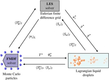
For the solution of filtered Eulerian carrier gas equations (2.7)–(2.9), any high-order numerical method may be used. The discretization procedure for this equation in this work is based on the fourth-order compact FD scheme and the third-order low-storage Runge–Kutta method. We use similar methods for DNS. Lagrangian spray equations are solved with numerical methods similar to those used for the FMDF, and the coupling terms are then calculated by volumetric averaging of droplet values. The SDEs are solved with the MC procedure. In this procedure, the filtered velocities are computed over the FD grid points and then interpolated from the FD grid points to the MC particle locations. As mentioned before, the spray coupling terms in the FMDF equation are calculated by averaging the droplet variables and feeding the FD data to MC particles. In the present hybrid methodology, the filtered values of variables such as temperature may be calculated from both FD grids and MC particles. This provides a unique opportunity for the assessment of the LES-FD and FMDF-MC parts of the LES/FMDF method. Mathematically, the filtered quantities computed from FD and MC data should be identical. Consistency of FMDF-MC and LES-FD implies numerical accuracy of both. To establish the consistency between FD and MC methods in reacting flows, the chemical source terms in the FD equations, which are closed in the FMDF formulation, are calculated from the MC particles. Different components of the LES/FMDF and its Eulerian–Lagrangian flow solver are shown in figure 1. The couplings between the carrier gas LES solver, the gas scalar FMDF solver and the Lagrangian liquid fuel droplet solver, implemented via a series of source/sink terms, are illustrated in figure 2. Figure 3 shows a sample flow simulated by the Eulerian FD method together with the Lagrangian MC particles and droplets.
A block diagram illustrating the couplings among the carrier gas LES solver, the gas scalar FMDF solver and the Lagrangian liquid fuel droplet solver.

Vorticity contours in the dump combustor, shown together with the Eulerian grids, Monte Carlo particles and Lagrangian droplets of the two-phase LES/FMDF flow solver.

4. Results
In this section, the computational implementation of the two-phase LES/FMDF model is discussed together with the numerical results for three flow configurations: (i) a spatially developing three-dimensional planar shear layer, (ii) a spray-controlled premixed dump combustor, and (iii) a double-swirl non-premixed spray combustor. DNS and LES/FMDF of non-reacting and reacting turbulent shear-layer or mixing-layer with and without spray are considered for a systematic assessment of the LES/FMDF and its submodels. The applicability of the two-phase LES/FMDF model to complex combustion systems is demonstrated by considering the premixed dump combustor and non-premixed swirl burner. The consistency and numerical accuracy of the two-phase LES/FMDF model are demonstrated for all three flows.
4.1. Shear layer
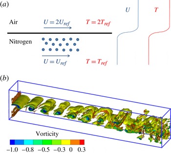
As mentioned above, DNS and LES of spatially developing shear layer or mixing layer with and without spray and combustion are conducted, mainly for a posteriori testing of the two-phase LES/FMDF model. Before considering the shear-layer flow with spray and combustion, it is necessary to establish the accuracy of the LES and its SGS models for the single-phase, non-reacting case. A schematic of the simulated mixing layer, the flow set-up and vorticity contours are shown in figure 4. Evidently, the lower-stream flow in the shear layer is a cold nitrogen stream with lower velocity of
 $V_{ref}$
and temperature of
 $T_{ref}$
. The upper stream has twice the lower-stream velocity of
 $2V_{ref}$
and is composed of air. To provide a suitable condition for droplet evaporation and combustion, the upper high-speed air flow is preheated to temperature
 $2T_{ref}$
. The Reynolds number based on the convective (average) free-stream velocity, inflow shear-layer thickness and cold flow viscosity is 100. To perturb the shear layer, three-dimensional turbulent velocity, density, temperature and pressure fluctuations are added to the mean flow variables at inflow. These fluctuating variables are obtained by DNS of compressible isotropic flow and are fed into the shear-layer flow with the convective shear-layer velocity. The amplitude of the fluctuating/turbulent velocity is set to be approximately 3 % of the lower-stream mean velocity. The vorticity contours in figure 4(a) clearly indicate that the flow becomes turbulent and three-dimensional at downstream locations, confirming that the added perturbation is sufficient to make the flow excited and turbulent at a reasonable distance from the inlet.
(a) Schematic view and (b) vorticity iso-levels in the simulated shear-layer flow.

To establish the accuracy of the numerical simulations, the shear-layer DNS is conducted on four different grids: G1,
 $325\times 64\times 24$
; G2,
 $650\times 128\times 48$
; G3,
 $975\times 192\times 72$
; G4,
 $1300\times 256\times 96$
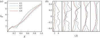
. Figure 5 shows the evolution of shear-layer thickness and Taylor micro-length-scale for all four grids. In this figure and all other figures in this paper,
 $X$
,
 $Y$
and
 $Z$
denote the normalized streamwise, cross-stream and spanwise locations. While the shear-layer thicknesses predicted by grids G2, G3 and G4 (figure 5
a) are close to each other, that simulated on grid G1 is shown to significantly overestimate the values predicted by grids G2, G3 and G4. The Taylor micro-length-scale values obtained from DNS data with all four grids at five different streamwise locations in figure 5(b) exhibit similar trends to those shown for the shear-layer thickness in figure 5(a). By increasing the grid resolution, the Taylor micro-length-scale values become closer to each other at all locations. The G3 and G4 values are shown to be particularly close. Based on these results, we believe that the simulations conducted by grid G4 are accurate, and thus we have conducted all of our DNS calculations on grid G4. The LES calculations are conducted on grid G1 for the same flow conditions as the DNS, using the dynamic Smagorinsky model for the SGS stresses. The SGS energy fluxes appearing in the filtered energy equation are modelled with a similar gradient-type closure.
The effect of grid resolution on the shear-layer variables: (a) mixing-layer thickness and (b) Taylor microscale.

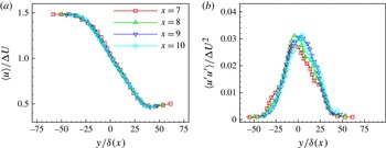
To confirm that the flow is adequately developed and is self-similar at downstream locations, DNS-predicted values of the mean and root-mean-square (r.m.s.) filtered axial velocity at different streamwise locations are compared in figures 6(a) and 6(b), respectively. The averaged values shown in this figure, and all other figures shown below, are calculated by both time averaging and space averaging in the spanwise (homogeneous) direction. The normalized mean velocity profiles at different distances, sufficiently far away from the inlet, are clearly similar. The normalized RMS profiles also become reasonably close at these axial locations, indicating that the shear layer becomes turbulent and self-similar.
Self-similarity in the simulated shear layer on grid G4: (a) mean (time-averaged) axial velocity and (b) r.m.s. of axial velocity.

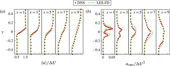
Comparison of LES and DNS velocity statistics for the mixing layer: (a) time-averaged axial velocity and (b) r.m.s. of axial velocity.

The LES predictions of the shear layer statistics are also in good agreement with the DNS data, indicating the reliability of LES and its SGS models. This is shown in figure 7, where the normalized mean and r.m.s. values of the axial velocity obtained by DNS and LES are compared. These results are for non-reacting (but non-isothermal) single-phase shear-layer flow without any droplets. Clearly, the flow is highly asymmetric (mainly due to non-isothermal conditions) and the velocity statistics change significantly in a relatively short distance along the flow, yet the LES model is able to capture these variations with reasonable accuracy. It was important for this to be demonstrated for the single-phase non-reacting flows first before testing the accuracy of the LES/FMDF model for two-phase reacting flows.
The ability of the LES/FMDF model to predict two-phase flows is assessed by conducting non-reacting and reacting droplet-laden simulations. For these two-phase flow simulations, the lower, low-speed, nitrogen shear-layer stream is randomly filled with decane liquid droplets with initially uniform diameters of
 $10\ {\rm\mu}\text{m}$
. Decane droplets are continuously and randomly fed at the lower-stream flow inlet to establish the steady condition with a constant (liquid to gas) mass loading ratio (MLR) of
 $\frac{1}{5}$
.
An important issue in a hybrid mathematical/numerical scheme such as the LES/FMDF is the consistency of its sub-components. We establish the consistency here by comparing the results obtained by the FMDF and its Lagrangian Monte Carlo solver with those obtained by the finite difference solution of filtered LES equations. This is done for (i) non-reacting flows without spray, (ii) non-reacting flows with spray and droplet evaporation, (iii) reacting flows with fuel spray and evaporation. In the discussion below, the scalar (temperature and species mass fraction) values generated by the finite difference method on the Eulerian grid points are denoted by FD and the results obtained by ensemble averaging of the Monte Carlo particles over an ensemble domain or volume are denoted by MC. The consistency of FD and MC methods indicates the numerical accuracy of both, and the reliability of the hybrid LES/FMDF methodology. We like to emphasize that it is possible to compare the FD results with the MC results in our reacting simulations because the corresponding reaction terms in FD are computed from the MC particles. These terms are not closed in the filtered equations and cannot be computed with conventional LES methods.
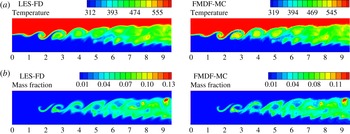
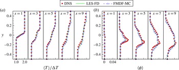
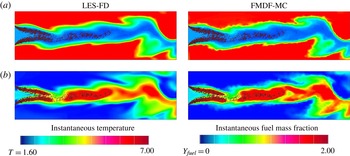
Our non-isothermal, single-phase non-reacting shear-layer results (not shown) indicate that the filtered turbulent temperature and density calculated from the LES-FD and FMDF-MC data are similar, confirming the numerical accuracy of the LES/FMDF flow solver when there is no spray, droplet evaporation or combustion. The LES-FD and FMDF-MC results are also consistent and numerically accurate when there is spray and/or combustion. Figure 8(a,b) shows the contours of the instantaneous filtered temperature and evaporated liquid mass fraction for the two-phase, non-reacting simulations as predicted by these two methods. A high level of evaporation occurs at the shear layer, where the nitrogen gas surrounding the droplets is warmed up by the air stream. There is a significant heat and mass transfer between the liquid and gas phases in these regions of the flow due to heating of droplets and evaporation. Nevertheless, the LES-FD and FMDF-MC contours stay very similar and fully consistent throughout the flow at all times. The time-averaged values of the gas temperature and evaporated fuel mass fraction as predicted by the LES-FD and FMDF-MC parts of the LES/FMDF at different streamwise locations are compared with each other and also with the DNS data in figure 9. Similar to the results shown in figure 8, the LES-FD and FMDF-MC predictions of mean gas temperature and evaporated liquid mass fraction are in very good agreement with each other and with those obtained from the DNS data. The good consistency between LES-FD and FMDF-MC results indicates the accuracy of the computational algorithm and the numerical methods employed in the LES/FMDF for the simulated evaporating droplet-laden non-isothermal system. The good comparison between LES and DNS results indicates the accuracy of the submodels employed in the LES/FMDF.
Comparison of LES-FD and FMDF-MC results for the evaporating mixing layer without combustion: (a) time-averaged temperature and (b) time-averaged fuel mass fraction.

Comparison of LES-FD, FMDF-MC and DNS results for the evaporating case without combustion: (a) time-averaged temperature and (b) time-averaged fuel mass fraction.

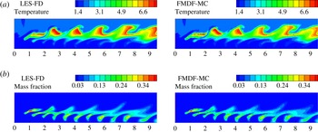
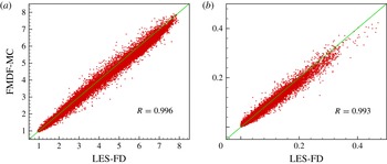
The combustion of the evaporated fuel (decane) with the air, occurring in the regions with high temperature and well-mixed evaporated fuel–air mixture, significantly affects the growth rate of the shear layer and the vorticity/turbulence field. While almost all the evaporated fuel in the shear layer reacts, the gas fuel in regions between the shear layer and lower-speed (cold) flow stream remains unburned. These are illustrated in figure 10, where the instantaneous contours of LES-FD and FMDF-MC temperatures and evaporated liquid fuel mass fractions are shown. The similarity of the LES-FD and FMDF-MC results is better shown in figure 11. This figure shows the scatter values of the filtered FD and MC temperatures for most of the active flow domain. Despite the very strong effect of the combustion on the shear layer, the LES-FD and FMDF-MC results remain consistent and very similar. The reason for this similarity is the numerical accuracy of the FD and MC methods and also the fact that the reaction source/sink terms in the FD equations are computed from the MC particles. As mentioned before, the reaction terms are closed in the FMDF formulation and can be accurately computed from the MC particles but they are not closed in the LES equations. The droplet mass, momentum and energy phase-change (evaporation) terms must also have been computed consistently from the MC particles, otherwise we could not get such similar results from both methods.
Comparison of LES-FD and FMDF-MC results for the evaporating case with combustion: (a) two-dimensional contours of temperature and (b) two-dimensional contours of fuel mass fraction.

Scatter plots of filtered gas temperature and fuel mass fraction in reacting shear-layer flow as obtained from the LES-FD and FMDF-MC parts of the LES/FMDF model: (a) temperature and (b) evaporated fuel mass fraction.

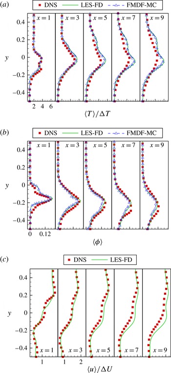
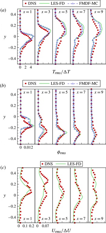
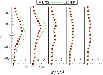
Figure 12 shows the mean (time-averaged) values of the filtered temperature, the evaporated fuel mass fraction and the axial velocity as obtained by DNS and LES/FMDF in the two-phase reacting mixing layer at different axial locations. The temperature and fuel mass fraction plots are obtained from the LES-FD and FMDF-MC parts of the LES/FMDF model. It is clear that these two parts of the model again generate very similar and consistent results. It is also observed in figure 12 that the mean values of the filtered temperature, fuel mass fraction and velocity are accurately computed by the two-phase LES/FMDF model when compared with the DNS data at all spatial locations. Not only are the mean values of the turbulent variables predicted by the two parts of the LES/FMDF model similar, and compare well with the DNS data, but the r.m.s. values are also consistent and accurate. This is shown in figure 13. This figure shows the r.m.s. of the three turbulent variables obtained from LES/FMDF and DNS data at different axial locations. Clearly, the r.m.s. values of these variables are also consistent and well predicted by the LES/FMDF as compared to DNS. Comparison of the DNS and LES turbulent kinetic energy (TKE) in figure 14 also indicates that the LES and its SGS models are able to capture well the exact TKE trends computed by DNS.
Comparison of LES-FD, FMDF-MC and DNS results for the evaporating mixing layer with combustion: (a) mean (time-averaged) normalized temperature, (b) mean fuel mass fraction, and (c) mean velocity.

Comparison of LES-FD, FMDF-MC and DNS results for the evaporating mixing layer with combustion: (a) r.m.s. of temperature, (b) r.m.s. of fuel mass fraction, and (c) r.m.s. of velocity.

Comparison of LES-resolved TKE and DNS turbulent kinetic energy for the evaporating mixing layer with combustion.

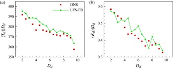
In addition to predicting the gas-phase turbulent velocity and scalar statistics, our new two-phase LES/FMDF model is also able to compute the droplet values with good accuracy. This is demonstrated in figure 15, where the conditional averaged values of the droplet temperature and droplet kinetic energy, conditioned on the droplet size as obtained from DNS and LES data for the mixing layer with evaporation and combustion, are compared at different droplet sizes. Clearly there is good comparison between DNS and LES results. These results (and those shown above and also those not shown in this paper) indicate that, despite the complexity of the simulated turbulence, the droplet transport, the non-equilibrium evaporation, the finite rate reaction, and all mass, momentum and energy interactions between phases, the new two-phase LES/FMDF model is consistent and is able to give good predictions of the DNS results under all conditions tested. This indicates the reliability and accuracy of LES/FMDF and its subcomponents and submodels.
Comparison of LES and DNS results for the evaporating mixing layer with combustion. (a) Conditional averaged droplet temperature, conditioned on the droplet size. (b) Normalized conditional droplet kinetic energy, conditioned on the droplet size.

4.2. Dump combustor and swirl burner
In this section, LES/FMDF results are presented for two other flows, both more complex than the shear layer. The first flow is a lean premixed dump combustor (Hsu, Pang & Yu Reference Hsu, Pang and Yu2001), affected or controlled by two liquid fuel sprays. The second flow is a non-premixed swirl spray burner (Linck et al. Reference Linck, Gupta, Bourhis and Yu2006). These flows are considered to establish the consistency, numerical accuracy and applicability of the LES/FMDF model to more complex combustion systems. There is limited information concerning the flow conditions, spray, etc., for these experiments. Consequently, direct (quantitative) comparison with these experiments is not possible and is not attempted. Nevertheless, our results are qualitatively similar and reproduce the trends seen in the experiments.
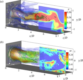
Figure 16 shows the injected fuel droplets together with the three-dimensional instantaneous isosurfaces of the vorticity and density for the simulated dump combustor. In the dump combustor experiment, the established lean premixed air–fuel flame in the combustor is modified by injection of a relatively small amount of liquid fuel (figures 3 and 16). The equivalence ratio of the inflow gas is 0.7 and the flow Reynolds number, calculated based on the inlet diameter and the mean bulk inlet velocity, is 38 580 in both experiment and LES. We have simulated this flow with and without (heptane) fuel spray evaporation and combustion.
Iso-contours of the instantaneous filtered values as obtained by the two-phase FMDF: (a) density and (b) vorticity.

In a spray combustion system, the evaporation of liquid fuel droplets has two major effects on the flow and flame. First, it provides gaseous fuel for the chemical reaction and sustains or promotes combustion. Second, the drag, heat transfer and evaporation of droplets significantly change the temperature, turbulence and species concentrations in the carrier gas. These two effects often counter each other in the simulated spray combustor. The net result is dependent on the premixed gas equivalence ratio, and spray parameters and features such as the spray angle and droplet size and velocity distribution. Our results indicate that despite the cooling effect of the droplets on the flame, the added liquid fuel quickly increases the flame temperature away from the combustor centreline even at locations close to sprays and combustor inlet. Without sprays, the fuel distribution peaks close to the centreline where the temperature is relatively low and there is no combustion. But the added liquid fuel increases the gaseous fuel concentration closer to the wall since only a fraction of the evaporated fuel at this location burns. Droplets that survive the evaporation and combustion concentrate in the centre of the combustor (figure 18). Their cooling effect keeps the temperature at this location relatively low in the entire combustor.
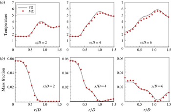
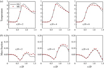
Despite the very significant effect that the spray/droplet and flow parameters have on the flame and flow structure, we have found the FMDF-MC predictions of the instantaneous temperature and fuel mass fraction to be close to those of LES-FD in the entire combustor for all cases studied. Figure 17, for example, shows the radial variations of the filtered temperature and the evaporated fuel mass fraction obtained from the Eulerian FD and Lagrangian MC data in the dump combustor at three locations from the inlet when there is combustion but no liquid-fuel spray. Evidently, the FMDF-MC and LES-FD predictions are in very good agreement at all locations. The corresponding temperature and mass fraction contours (not shown) also indicate a nearly perfect match between LES-FD and FMDF-MC results, again demonstrating the numerical accuracy of the LES/FMDF method for single-phase premixed flames. For the two-phase reacting case with all spray and combustion effects present, the contour and radial plots of the temperature and fuel mass fraction in figures 18 and 19 once again indicate good consistency between FD and MC results. Comparison between the case without spray (figure 17) and the case with spray evaporation and liquid fuel combustion (figure 19) indicates that the sprays indeed have a very significant effect on the gas mass, momentum and energy fields in the combustor.
Radial variations of the instantaneous values of filtered temperature and fuel mass fraction at different axial (
 $x$
) locations in the premixed dump combustor without fuel spray. Monte Carlo values are represented by MC and FD values by FD. (a) Temperature and (b) fuel mass fraction.

Iso-contours of the instantaneous filtered temperature and fuel mass fraction as obtained by LES/FDMF: (a) LES-FD and FMDF-MC values of temperature and (b) LES-FD and FMDF-MC values of mass fraction.

Radial variations of the instantaneous values of filtered temperature and fuel mass fraction at different axial (
 $x$
) locations in the premixed dump combustor with fuel spray. Monte Carlo values are represented by MC and FD values by FD.

For further assessment of the LES/FMDF model, simulations of turbulent flows in a double-swirl spray burner (Linck et al.
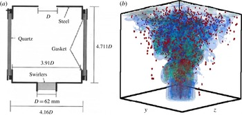
Reference Linck, Gupta, Bourhis and Yu2006) have also been conducted. A schematic picture of the combustion chamber is shown together with contours of the vorticity and droplets in figure 20. This is a non-premixed combustion system, completely controlled by the spray, as opposed to the previous dump combustor system which was premixed and just partially affected by the spray. The swirl number
 $S=G_{{\it\theta}}/(R_{0}G_{a})$
(where
 $R_{0}$
,
 $G_{{\it\theta}}$
and
 $G_{a}$
are the outer radius of the swirler, the axial flux of angular momentum and the axial flux of axial momentum, respectively) characterizes the degree of tangential momentum or swirl in the inflow air and has a significant effect on the stability and structure of the flame. For the vane angle of
 $45^{\circ }/50^{\circ }$
(inner/outer annulus) used here, the corresponding swirl numbers are
 $0.8/1.0$
for the inner/outer annulus.
(a) Schematic of a double-swirl stabilized spray burner. (b) The instantaneous vorticity iso-surfaces and fuel droplet distribution in the double-swirl spray burner.

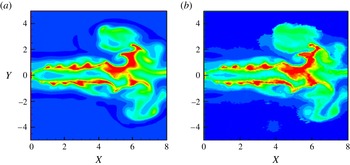
One of the most important parameters that affects the combustion and flow in the double-swirl burner is the MLR, which is defined as the ratio of fuel flow rate to air flow rate. It is obvious that for significant sprayed fuel and very high MLR the flame will be turned off due to excessive richness of the local fuel–air mixture and the added cooling effect of spray. Furthermore, due to two-way momentum interactions between droplet and carrier gas, the turbulence in the carrier gas with more droplets or larger MLR will be damped significantly with or without combustion, even when the flame is close to extinction. Despite the very different flow and combustion structures at different MLRs, the LES-FD and FMDF-MC parts of the LES/FMDF remain fully consistent. This is very important and indicates the accuracy of the LES/FMDF model. To show the consistency, the instantaneous contours of the filtered temperature, obtained from LES-FD and FMDF-MC data for a MLR value, are compared in figure 21. Evidently, the MC and FD results are very close.
Contours of the instantaneous filtered temperature in the double-swirl burner as obtained by LES/FDMF: (a) LES-FD and (b) FMDF-MC.

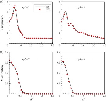
To better assess the consistency of subcomponents of LES/FMDF in the non-premixed double-swirl burner, the radial variations of the filtered temperature and fuel mass fraction obtained by the two parts of the model are compared in figure 22. Evidently, for both the temperature and the fuel mass fraction, the FMDF-MC predictions are very close to those of LES-FD at all locations and times, again indicating the consistency of the multi-phase LES/FMDF methodology and its numerical solver for the swirl burner. Based on these results and those shown before, we conclude that the FMDF-MC and LES-FD components in the two-phase LES/FMDF method are both mathematically correct and numerically accurate for all tested flow, spray and combustion conditions. Again, we note that in our simulations the reaction source/sink terms in the LES-FD equations are obtained from the MC particles. This is for the testing of the numerical methods and for showing the consistency. Such information is not available in standard LES methods.
The averaged gas temperature and fuel mass fraction in the double-swirl spray burner as obtained from the FD and MC parts of the LES/FMDF model: (a) temperature and (b) fuel mass fraction.

5. Summary and conclusions
A probability density function model, termed the FMDF, is developed and tested for large-eddy simulation (LES) of droplet-laden, two-phase turbulent reacting flows. The numerical solution of the two-phase LES/FMDF is based on a Lagrangian–Eulerian–Lagrangian mathematical/computational methodology. In this methodology, a high-order finite difference (FD) scheme is used for simulations of the Eulerian velocity field but the gas-phase scalars (temperature and species mass fractions) are obtained from the FMDF with a Lagrangian Monte Carlo (MC) method. The liquid spray is simulated with a Lagrangian model which allows two-way mass, momentum and energy coupling between phases. The consistency of the two-phase FMDF and the performance of submodels employed in the FMDF transport equation are assessed by comparison between the carrier gas results obtained from the MC particles (FMDF-MC) and finite difference grids (LES-FD) data for three flows: (i) a spatially developing reacting mixing layer with and without sprays, (ii) a lean premixed dump combustor controlled by small amount of sprayed liquid fuel, and (iii) a spray-controlled non-premixed double-swirl burner. In order to validate the new two-phase LES/FMDF model, the results of this model were also compared with the DNS data for non-reacting and reacting two-phase mixing layers. It is shown that the instantaneous and time-averaged mean and r.m.s. values of the filtered temperature and fuel mass fraction obtained from the LES-FD and FMDF-MC data are consistent and compare well with the DNS data for this flow. Our results also indicate that the new two-phase LES/FMDF model can capture the main features of the premixed dump combustor and the non-premixed swirl burner with consistent and similar LES-FD and FMDF-MC predictions for various flow/spray/combustion conditions. All of these results indicate that the new two-phase LES/FMDF model is a reliable and affordable model for detailed calculations of turbulent spray combustion. The model is based on a robust mathematical/computational framework and can be continuously improved and applied to increasingly complex multiphase reacting systems without having to change its basic framework.
It should be stated here that this mathematical formulation and computational method are applicable to dilute sprays, which are characterized by small heavy droplets with low volume fraction. As the number of droplets or their sizes increase, the droplet–droplet collision and liquid volume fraction effects become more important, and the submodels used for the spray should be improved. The volume fraction effects should also be included in the LES/FMDF formulation for the gas variables. When the liquid/droplet size becomes comparable to or larger than the Eulerian grid size, we need to use Eulerian–Eulerian methods and interface tracking schemes to capture the interface between liquid and gas phases directly.
Acknowledgements
This work was sponsored by the National Science Foundation under grant CTS0092665. Additional support was provided by the US Department of Energy under agreement DE-FC26-07NT43278. Computational resources were provided by the High Performance Computing Center at Michigan State University.
Appendix A
In the hybrid LES/FMDF methodology, it is not often possible to directly use the energy or temperature calculated from the Lagrangian MC particles in the compressible gas dynamics LES-FD equations due to noise introduced by the Lagrangian MC particles. A common practice (Jaberi et al.
Reference Jaberi, Colucci, James, Givi and Pope1999) is to solve a sensible enthalpy equation by the FD method with the reaction terms computed from the FMDF-MC. In most published papers on numerical study of compressible two-phase flows with phase coupling (e.g. Miller & Bellan Reference Miller and Bellan1999 and Almeida & Jaberi Reference Almeida and Jaberi2006), a transport equation like the following equation for the total energy
 $E=\sum _{{\it\alpha}=1}^{N_{s}}h_{{\it\alpha}}Y_{{\it\alpha}}-p/{\it\rho}+u_{i}u_{i}/2$
is considered:
 $$\begin{eqnarray}\frac{\partial {\it\rho}E}{\partial t}+\frac{\partial {\it\rho}u_{i}E}{\partial x_{i}}=-\frac{\partial pu_{i}}{\partial x_{i}}+\frac{\partial u_{j}{\it\tau}_{ij}}{\partial x_{i}}-\frac{\partial q_{i}}{\partial x_{i}}+S_{E}.\end{eqnarray}$$
In this equation, the chemical reaction effect is implicitly included through species enthalpy
 $h_{{\it\alpha}}$
. To derive a ‘sensible’ enthalpy equation for the two-phase LES/FMDF, the kinetic energy equation is subtracted first from the total energy equation. The resulting total enthalpy
 $H=\sum _{{\it\alpha}=1}^{N}h_{{\it\alpha}}y_{{\it\alpha}}$
equation is
 $$\begin{eqnarray}\frac{\partial {\it\rho}H}{\partial t}+\frac{\partial {\it\rho}u_{i}H}{\partial x_{i}}=-\frac{\partial }{\partial x_{i}}\left(\frac{-{\it\mu}}{\mathit{Pr}}\frac{\partial H}{\partial x_{i}}\right)+S_{H},\end{eqnarray}$$
where the pressure derivative and viscous dissipation terms are ignored, as is usually done in low-Mach-number flows (Pope Reference Pope1985). In the above equation,
 $S_{H}=S_{E}-u_{i}S_{ui}+(u_{i}u_{i})/2S_{{\it\rho}}$
.
The species’ mass fraction (
 $y_{{\it\alpha}}$
) equations for a two-phase reacting flow with fuel droplet evaporation is written as
 $$\begin{eqnarray}\frac{\partial {\it\rho}Y_{{\it\alpha}}}{\partial t}+\frac{\partial {\it\rho}u_{i}Y_{{\it\alpha}}}{\partial x_{i}}=-\frac{\partial }{\partial x_{i}}\left(\frac{-{\it\mu}}{\mathit{Pr}}\frac{\partial Y_{{\it\alpha}}}{\partial x_{i}}\right)+{\it\rho}\dot{{\it\omega}}_{{\it\alpha}}+S_{{\it\rho}}{\it\delta}_{1{\it\alpha}},\end{eqnarray}$$
where for
 ${\it\alpha}=1$
, the scalar is the gas fuel and the
 $S_{{\it\rho}}{\it\delta}_{1{\it\alpha}}$
term indicates that the droplet evaporation only increases the fuel mass fraction. The fuel in the gas mixture has two parts: one is the original ‘dry’ fuel and the other is the ‘vapour’ fuel from the liquid evaporation. The total fuel gas is
 $Y_{1}=Y_{fd}+Y_{fv}$
, where
 $Y_{fd}$
and
 $Y_{fv}$
are the mass fractions of dry and vapour fuel, respectively. The dry and vapour fuel can have different enthalpies (i.e.
 $h_{1}^{0}=h_{fd}^{0}\neq h_{v}^{0}$
). The vapour fuel has to be mixed into dry fuel before combustion. Consequently, (A 3) can be split into two set of equations
 $$\begin{eqnarray}\frac{\partial {\it\rho}Y_{{\it\alpha}}}{\partial t}+\frac{\partial {\it\rho}u_{i}Y_{{\it\alpha}}}{\partial x_{i}}=-\frac{\partial }{\partial x_{i}}\left(\frac{-{\it\mu}}{\mathit{Pr}}\frac{\partial Y_{{\it\alpha}}}{\partial x_{i}}\right)+{\it\rho}\dot{{\it\omega}}_{{\it\alpha}}\quad \text{for}\ {\it\alpha}\neq 1,\end{eqnarray}$$
and
 $$\begin{eqnarray}\begin{array}{@{}l@{}}\displaystyle \frac{\partial {\it\rho}Y_{fd}}{\partial t}+\frac{\partial {\it\rho}u_{i}Y_{fd}}{\partial x_{i}}=-\frac{\partial }{\partial x_{i}}\left(\frac{-{\it\mu}}{\mathit{Pr}}\frac{\partial Y_{fd}}{\partial x_{i}}\right)+{\it\rho}\dot{{\it\omega}}_{{\it\alpha}}\\ \displaystyle \frac{\partial {\it\rho}Y_{fv}}{\partial t}+\frac{\partial {\it\rho}u_{i}Y_{fv}}{\partial x_{i}}=-\frac{\partial }{\partial x_{i}}\left(\frac{-{\it\mu}}{\mathit{Pr}}\frac{\partial Y_{fv}}{\partial x_{i}}\right)+S_{{\it\rho}}\end{array}\quad \text{for}\ {\it\alpha}=1.\end{eqnarray}$$
Now the total enthalpy can be rewritten as
 $$\begin{eqnarray}\displaystyle H=C_{p}T+\mathop{\sum }\limits_{{\it\alpha}=2}^{N_{s}}h_{{\it\alpha}}^{0}Y_{{\it\alpha}}+Y_{fd}h_{1}^{0}+Y_{fv}h_{v}^{0}, & & \displaystyle\end{eqnarray}$$
where
 $h_{fd}=h_{1}^{0}+C_{p,fd}T,h_{fv}=h_{v}^{0}+C_{p,fv}T,C_{p,fd}=C_{p,fv}=C_{p,1}$
. The transport equation for sensible enthalpy
 $h$
, which is derived from (A 4), (A 5) and (A 2), is
 $$\begin{eqnarray}\frac{\partial {\it\rho}h}{\partial t}+\frac{\partial {\it\rho}u_{i}h}{\partial x_{i}}=\frac{\partial }{\partial x_{i}}\left(\frac{-{\it\mu}}{\mathit{Pr}}\frac{\partial h}{\partial x_{i}}\right)-\mathop{\sum }\limits_{{\it\alpha}=1}^{N_{s}}h_{{\it\alpha}}^{0}{\it\rho}\dot{{\it\omega}}_{{\it\alpha}}+S_{h},\end{eqnarray}$$
where
 $S_{h}=S_{H}-S_{{\it\rho}}h_{v}^{0}=S_{E}-u_{i}S_{ui}+((u_{i}u_{i})/2-h_{v}^{0})S_{{\it\rho}}$
. The chemical reaction term
 $\dot{{\it\omega}}_{{\it\alpha}}$
and the droplet term
 $S_{h}$
both explicitly appear on the right-hand side of (A 7).
The species mass fraction equation (A 3) and sensible enthalpy equation (A 7) are written together as one equation for the scalar
 ${\it\phi}_{{\it\alpha}}$
,
 $$\begin{eqnarray}\frac{\partial {\it\rho}{\it\phi}_{{\it\alpha}}}{\partial t}+\frac{\partial {\it\rho}u_{i}{\it\phi}_{{\it\alpha}}}{\partial x_{i}}=-\frac{\partial J_{i}^{{\it\alpha}}}{\partial x_{i}}+S_{R}^{{\it\alpha}}+S_{S}^{{\it\alpha}},\quad {\it\alpha}=1,\dots ,N_{s}+1,\end{eqnarray}$$
where
 $$\begin{eqnarray}\left.\begin{array}{@{}llll@{}}{\it\phi}_{{\it\alpha}}\equiv Y_{{\it\alpha}}, & S_{R}^{{\it\alpha}}={\it\rho}\dot{{\it\omega}}_{{\it\alpha}}, & S_{S}^{{\it\alpha}}=S_{{\it\rho}}{\it\delta}_{1{\it\alpha}} & \text{for}\ {\it\alpha}=1,\dots ,N_{s},\\ \displaystyle {\it\phi}_{{\it\alpha}}\equiv h, & \displaystyle S_{R}^{{\it\alpha}}=-\mathop{\sum }\limits_{{\it\alpha}=1}^{N_{s}}h_{{\it\alpha}}^{0}{\it\rho}\dot{{\it\omega}}_{{\it\alpha}}, & S_{S}^{{\it\alpha}}=S_{h} & \text{for}\ {\it\alpha}=N_{s}+1,\end{array}\right\}\end{eqnarray}$$
and
 $$\begin{eqnarray}J_{i}^{{\it\alpha}}=\frac{{\it\mu}}{\mathit{Pr}\,Le_{{\it\alpha}}}\frac{\partial {\it\phi}_{{\it\alpha}}}{\partial x_{i}}=\frac{{\it\mu}}{\mathit{Sc}}\frac{\partial {\it\phi}_{{\it\alpha}}}{\partial x_{i}}=-{\it\rho}{\it\Gamma}\frac{\partial {\it\phi}_{{\it\alpha}}}{\partial x_{i}}.\end{eqnarray}$$
Appendix B
The scalar FMDF is a function of the ‘fine-grained’ density
 ${\it\xi}$
and the filter function
 $G$
as
 $$\begin{eqnarray}P_{L}({\it\bf\Psi};\boldsymbol{x},t)=\int _{-\infty }^{+\infty }{\it\rho}(\boldsymbol{x}^{\prime },t){\it\xi}[{\it\bf\Psi},{\it\bf\Phi}(\boldsymbol{x}^{\prime },t)]G(\boldsymbol{x}^{\prime }-\boldsymbol{x})\text{d}\boldsymbol{x}^{\prime },\end{eqnarray}$$
where
 $$\begin{eqnarray}\displaystyle {\it\xi}[{\it\bf\Psi},{\it\bf\Phi}(\boldsymbol{x},t)]={\it\delta}({\it\bf\Psi}-{\it\bf\Phi}(\boldsymbol{x},t))=\prod _{{\it\alpha}=1}^{N_{s}+1}{\it\delta}({\it\psi}_{{\it\alpha}}-{\it\phi}_{{\it\alpha}}(\boldsymbol{x},t)). & & \displaystyle\end{eqnarray}$$
Following the method used by Jaberi et al. (Reference Jaberi, Colucci, James, Givi and Pope1999), the unfiltered (DNS) scalar equation (2.3) is used to derive the following transport equation for the fine-grained density:
 $$\begin{eqnarray}\displaystyle & & \displaystyle \displaystyle \frac{\partial {\it\rho}{\it\xi}({\it\bf\Psi},{\it\bf\Phi}(\boldsymbol{x},t))}{\partial t}+\frac{\partial {\it\rho}u_{i}{\it\xi}({\it\bf\Psi},{\it\bf\Phi}(\boldsymbol{x},t))}{\partial x_{i}}\nonumber\\ \displaystyle & & \displaystyle \displaystyle \quad =\frac{\partial J_{i}^{{\it\alpha}}}{\partial x_{i}}\frac{\partial {\it\delta}({\it\bf\Psi}-{\it\bf\Phi}(\boldsymbol{x},t))}{\partial {\it\psi}_{{\it\alpha}}}-\frac{\partial S_{R}^{{\it\alpha}}{\it\delta}({\it\bf\Psi}-{\it\bf\Phi}(\boldsymbol{x},t))}{\partial {\it\psi}_{{\it\alpha}}}-\,\frac{\partial S_{S}^{{\it\alpha}}{\it\delta}({\it\bf\Psi}-{\it\bf\Phi}(\boldsymbol{x},t))}{\partial {\it\psi}_{{\it\alpha}}}\nonumber\\ \displaystyle & & \displaystyle \displaystyle \qquad +\,\frac{\partial {\it\phi}_{{\it\alpha}}S_{{\it\rho}}{\it\delta}({\it\bf\Psi}-{\it\bf\Phi}(\boldsymbol{x},t))}{\partial {\it\psi}_{{\it\alpha}}}+\,S_{{\it\rho}}{\it\delta}({\it\bf\Psi}-{\it\bf\Phi}(\boldsymbol{x},t)).\end{eqnarray}$$
Each term in (B 3) is multiplied by the filter function
 $G(\boldsymbol{x}^{\prime }-\boldsymbol{x})$
, then integrated over
 $\boldsymbol{x}^{\prime }$
, term by term. For example, the first and second terms on the left-hand side become
 $$\begin{eqnarray}\displaystyle \int _{-\infty }^{+\infty }\frac{\partial {\it\rho}{\it\xi}({\it\bf\Psi},{\it\bf\Phi}(\boldsymbol{x},t))}{\partial t}G(\boldsymbol{x}^{\prime }-\boldsymbol{x})\text{d}\boldsymbol{x}^{\prime } & = & \displaystyle \frac{\partial }{\partial t}\int _{-\infty }^{+\infty }{\it\rho}{\it\xi}({\it\bf\Psi},{\it\bf\Phi}(\boldsymbol{x},t))G(\boldsymbol{x}^{\prime }-\boldsymbol{x})\text{d}\boldsymbol{x}^{\prime }\nonumber\\ \displaystyle & = & \displaystyle \frac{\partial P_{L}}{\partial t},\end{eqnarray}$$
 $$\begin{eqnarray}\displaystyle \int _{-\infty }^{+\infty }\frac{\partial {\it\rho}u_{i}{\it\xi}({\it\bf\Psi},{\it\bf\Phi}(\boldsymbol{x},t))}{\partial x_{i}}G(\boldsymbol{x}^{\prime }-\boldsymbol{x})\text{d}\boldsymbol{x}^{\prime } & = & \displaystyle \int _{-\infty }^{+\infty }{\it\rho}u_{i}{\it\xi}({\it\bf\Psi},{\it\bf\Phi}(\boldsymbol{x},t))\frac{\partial G(\boldsymbol{x}^{\prime }-\boldsymbol{x})}{\partial x_{i}}\text{d}\boldsymbol{x}^{\prime }\nonumber\\ \displaystyle & = & \displaystyle \frac{\partial }{\partial x_{i}}\left[\left\langle u_{i}(\boldsymbol{x},t)|{\it\bf\Psi}\right\rangle _{l}P_{L}\right]\!.\end{eqnarray}$$
By collecting all integrated terms, the final form of the exact transport equation for the two-phase FMDF is obtained:
 $$\begin{eqnarray}\displaystyle & & \displaystyle \frac{\partial P_{L}}{\partial t}+\frac{\partial }{\partial x_{i}}\left[\left\langle u_{i}(\boldsymbol{x},t)|{\it\bf\Psi}\right\rangle _{l}P_{L}\right]\nonumber\\ \displaystyle & & \displaystyle \quad =\frac{\partial }{\partial {\it\psi}_{{\it\alpha}}}\left[\left\langle \left.\frac{1}{\hat{{\it\rho}}({\it\bf\Phi})}\frac{\partial J_{i}^{{\it\alpha}}}{\partial x_{i}}\right|{\it\bf\Psi}\right\rangle _{l}P_{L}\right]-\frac{\partial }{\partial {\it\psi}_{{\it\alpha}}}\left[\left\langle \left.\frac{1}{\hat{{\it\rho}}({\it\bf\Phi})}{\hat{S}}_{R}^{{\it\alpha}}({\it\bf\Phi})\right|{\it\bf\Psi}\right\rangle _{l}P_{L}\right]\nonumber\\ \displaystyle & & \displaystyle \qquad -\,\frac{\partial }{\partial {\it\psi}_{{\it\alpha}}}\left[\left\langle \left.\frac{1}{\hat{{\it\rho}}({\it\bf\Phi})}{\hat{S}}_{S}^{{\it\alpha}}(\boldsymbol{x},t)\right|{\it\bf\Psi}\right\rangle _{l}P_{L}\right]+\frac{\partial }{\partial {\it\psi}_{{\it\alpha}}}\left[\left\langle \left.\frac{{\it\psi}_{{\it\alpha}}}{\hat{{\it\rho}}({\it\bf\Phi})}S_{{\it\rho}}(\boldsymbol{x},t)\right|{\it\bf\Psi}\right\rangle _{l}P_{L}\right]\nonumber\\ \displaystyle & & \displaystyle \qquad +\,\left\langle \left.\frac{S_{{\it\rho}}(\boldsymbol{x},t)}{\hat{{\it\rho}}({\it\bf\Phi})}\right|{\it\bf\Psi}\right\rangle _{l}P_{L}.\end{eqnarray}$$