






1 Introduction
Free liquid films – by free, we mean not confined between surfactant layers – are formed in various instances: they arise as a result of various jet impacts (Savart Reference Savart1833) or splashes in the form of ejecta sheets (Worthington Reference Worthington1908), they constitute the shell bounding surface bubbles (Blanchard Reference Blanchard1963), they can also be made on purpose through the extrusion of a liquid stream through a slit or annular thin jet in some spreading applications, in liquid propulsion devices or ornamental fountains (Dombrowski & Fraser Reference Dombrowski and Fraser1954). Liquid films are of course also involved in various flows of effluents down inclined plates and coating processes (Craster & Matar Reference Craster and Matar2009; Kalliadasis et al. Reference Kalliadasis, Ruyer-Quil, Scheid and Velarde2012).
Suspended liquid films, that is, those not lying on a solid surface, usually break up through their boundary. There, surface tension forces are unbalanced, pulling the liquid of the film into a receding rim, which undergoes a capillary instability, before forming ligaments and isolated drops (Ranz Reference Ranz1959; Huang Reference Huang1970; Lhuissier & Villermaux Reference Lhuissier and Villermaux2011). The receding motion can in some special instances be so fast that it triggers a shear instability with the surrounding environment (Lhuissier & Villermaux Reference Lhuissier and Villermaux2009b ).
Liquid films also happen to puncture far from their boundaries, nucleating a hole or a collection of adjacent holes on the plane of the film. These holes, if large enough in radius compared to the film thickness (Taylor & Michael Reference Taylor and Michael1973), may open irreversibly for the same reason mentioned above: at a hole edge, surface tension is no longer balanced. The criterion is identical for polymeric membranes (Ilton, DiMaria & Dalnoki-Veress Reference Ilton, Dimaria and Dalnoki-Veress2016) and is somewhat different for charged liquids (Betterton & Brenner Reference Betterton and Brenner1999). In a film of simple liquid, a hole radius, when initially large enough, grows in size at the constant Taylor–Culick speed
 $\sqrt{2\unicode[STIX]{x1D70E}/\unicode[STIX]{x1D70C}h}$
, where
 $\unicode[STIX]{x1D70C}$
is the liquid density,
 $\unicode[STIX]{x1D70E}$
its surface tension and
 $h$
the thickness of the film (Taylor Reference Taylor1959b
; Culick Reference Culick1960). If a hole has too small a radius, it heals (Courbin & Stone Reference Courbin and Stone2006).
While the sequence of phenomena occurring after a hole has been formed and opens in the plane of a film is well described and relatively well understood, the fundamental question of the hole nucleation process itself has been less explored. There are in fact many answers to this question, because there are many ways a film may puncture. We review them below, along with their domain of application, in order to motivate the need for a new study.
1.1 Extremely thin films: thermal fluctuations
Extremely small, thin objects are sensitive to thermal fluctuations. The minimal energy input to open a hole irreversibly is the surface energy
 $\unicode[STIX]{x1D70E}h^{2}$
(the hole radius must be of the order of the film thickness
 $h$
, or more), if
 $\unicode[STIX]{x1D70E}$
is the surface tension of the liquid. That energy can, provided a scenario leading to film rupture exists, be supplied by the quantum
 $k_{B}T$
from the liquid thermal bath, leading to
 $h\sim \sqrt{k_{B}T/\unicode[STIX]{x1D70E}}\approx 10^{-10}~\text{m}$
in water at ambient temperature, a critical film thickness of the order of the inter-atomic distances. This thermally activated puncture scenario may thus at most apply to extremely thin films, such as Newton black films (Casteletto et al.
Reference Casteletto, Cantat, Sarker, Bausch, Bonn and Meunier2003).
1.2 Very thin films: van der Waals forces
Intermolecular forces have different origins depending on whether the molecules are charged, permanently dipolar or dipolar by induction. These forces, called generically van der Waals forces (Israelachvili Reference Israelachvili1991), are attractive over a range of distances which compares to the size of the molecules itself, namely a few nanometres. The corresponding disjoining pressure
 $-A/h^{3}$
, where
 $A$
is a Hamaker constant (Derjaguin, Churaev & Muller Reference Derjaguin, Churaev and Muller1987), is responsible for puncturing very thin films up to a few tens of nanometres (Vrij Reference Vrij1966; Reiter Reference Reiter1992; Erneux & Davis Reference Erneux and Davis1993; Sharma & Reiter Reference Sharma and Reiter1996; Champougny et al.
Reference Champougny, Rio, Restagno and Scheid2017), but does not operate with much thicker films, despite the fact that appreciably thicker films, of the order of 200 nm (Thoroddsen et al.
Reference Thoroddsen, Thoraval, Takehara and Etoh2012), and even more (Nierstrasz & Frens Reference Nierstrasz and Frens1998) have been claimed to be sensitive to this effect.
1.3 External solicitations
A liquid film can be penetrated by a sharp solid object (with a radius of curvature smaller than the film thickness), a projectile (Courbin & Stone Reference Courbin and Stone2006), a concentrated air jet (Berendsen et al. Reference Berendsen, Zeegers, Kruis, Riepen and Darhuber2012; Lhuissier, Brunet & Dorbolo Reference Lhuissier, Brunet and Dorbolo2016), a focused laser beam (Wedershoven et al. Reference Wedershoven, Berendsen, Zeegers and Darhuber2015) or a spark (McEntee & Mysels Reference McEntee and Mysels1969; Lhuissier & Villermaux Reference Lhuissier and Villermaux2009a ), whose action is applied for a sufficiently long time. Like all fragile objects, liquid films are also sensitive to the unsteadiness of their environment. The application of a pressure gradient, or pressure difference across a film sets it in motion, and the corresponding acceleration may, because the film is a density interface when surrounded by a gas, lead to destabilisation through a Rayleigh–Taylor mechanism. An impulsive pressure wave (Bremond & Villermaux Reference Bremond and Villermaux2005), or a violent explosion (Vledouts et al. Reference Vledouts, Quinard, Vandenberghe and Villermaux2016) causes the film, accelerated perpendicular to its plane, to grow thickness modulations which ultimately cause its puncture with a well prescribed wavelength. The same phenomenon is responsible for the crumpling of liquid bells, and the formation of transverse indentations at the edge of flapping liquid sheets (Lhuissier & Villermaux Reference Lhuissier and Villermaux2012b ). It may affect films of arbitrary thicknesses: the studies just mentioned had films of thickness from microns to tens of microns.
1.4 Internal flaws and defects
Solid hydrophobic particles introduced into a film can, when their size compares with the film thickness, lead to its rupture as they force the two interfaces of the film to pinch at the surface of the particle. Anti-foaming agents have taken advantage of this effect for a long time (Garrett Reference Garrett1992; de Gennes Reference de Gennes1998). However, flaws, impurities or defects in the liquid may not be solid. Immiscible oil droplets (Dombrowski & Fraser Reference Dombrowski and Fraser1954), or bubbles (Lhuissier & Villermaux Reference Lhuissier and Villermaux2013) also act as efficient hole nucleation sites in water films for precise reasons that remain largely elusive. Denkov (Reference Denkov2004) notes that when by chance an oil droplet reaches an aqueous interface, the resulting surface tension contrast (oils have usually a weaker surface tension than water) drives a well-defined outward superficial flow. Vernay, Ramos & Ligoure (Reference Vernay, Ramos and Ligoure2015), adapting this result to a radially expanding liquid sheet loaded with partially miscible oil droplets, argue that it is responsible for the film piercing, which they do observe experimentally. We will come back on this point.
1.5 Surface inhomogeneities and Marangoni stresses
Chemical and temperature inhomogeneities at the surface of a liquid translate into inhomogeneities of surface tension. The corresponding Marangoni surface stress (Marangoni Reference Marangoni1878) is communicated to the bulk of the liquid by viscosity in a way that can be dramatic when the liquid is shallow as in films (Scriven & Sternling Reference Scriven and Sternling1960). In the Bénard problem of a liquid layer heated from below, for instance, the mean temperature decays from the hot plate to the liquid free surface. Since surface tension of a liquid typically decreases with temperature, this gradient yields a surface shear stress when the interface is distorted, setting the liquid into motion towards the cooler areas, where the surface tension is higher (Levich & Krylov Reference Levich and Krylov1969). There, the film thickens when at the same time the flow away from the hotter regions results in film thinning. Any initial disturbance of the film thickness or of the interface temperature is thus amplified. This instability may lead to film rupture, and local drying of the heating plate (Vanhook et al. Reference Vanhook, Schatz, Swift, McCormick and Swinney1997; Boos & Thess Reference Boos and Thess1999; Kabova et al. Reference Kabova, Alexeev, Gambaryan-Roisman and Stephan2006), namely the analogue of hole formation. This effect, which may also be due to differential evaporation in mixtures (Guéna, Poulard & Cazabat Reference Guéna, Poulard and Cazabat2007) is, for this reason, used as an efficient cleaning process (Leenaars, Huethorst & Van Oekel Reference Leenaars, Huethorst and Van Oekel1990; Matar & Craster Reference Matar and Craster2001). Other experiments of Marangoni stress induced spreading flows include those of Roché et al. (Reference Roché, Li, Griffiths, Le Roux, Cantat, Saint-Jalmes and Stone2014) and Hernández-Sánchez, Eddi & Snoeijer (Reference Hernández-Sánchez, Eddi and Snoeijer2015) suggesting that this kind of mechanism can affect films up to a millimetre thick.
1.6 The enigma of thick, spontaneously puncturing films
Yet, if the case of extremely thin or very thin films (§§ 1.1 and 1.2) is satisfactorily understood, the case of thick films, being sensitive to neither thermal fluctuations nor to a disjoining pressure, remains an enigma in the absence of sustained temperature or pollutant concentration gradient (§ 1.5). Even the precise role of defects (§ 1.4), when they are temperature or soluble chemical agent spots localised in space in, or at the surface of the film, needs to be clarified. A fundamental issue is to know whether a localised surface inhomogeneity spontaneously leads to film rupture in a finite time (Bowen & Tilley Reference Bowen and Tilley2013), besides the possible role of surfactants (Jensen & Grotberg Reference Jensen and Grotberg1992, Reference Jensen and Grotberg1993). The problem is particularly acute for liquid films with high superficial energy like water (Lhuissier & Villermaux Reference Lhuissier and Villermaux2012a ) or mercury (Dombrowski & Fraser Reference Dombrowski and Fraser1954) whose surface is easily contaminated by ambient pollutants, those films being known to puncture spontaneously, for yet unknown reasons (see figure 1), even if thick in the sense of the above classification.
A free mercury film puncturing spontaneously, adapted from Dombrowski & Fraser (Reference Dombrowski and Fraser1954). Waves (A), precursors (B), folds (C) of unknown origin are seen on the film, causing the opening of holes (D).

We present new facts regarding this issue interpreted by an original analysis, suggesting that a sufficiently large and strong chemical or thermal inhomogeneity deposited on a thick film can lead to its catastrophic puncture.
The method for preparing thick, stationary clean liquid films is first presented in § 2. In this section also, we explain how we perturb the surface properties of films, as well as the imaging tools we use to document the piercing phenomenon, which we illustrate qualitatively. A possible mechanism explaining the self-amplification of surface defects is presented in § 3. In order to examine its relevance, we come back to precise experiments in § 4, which we analyse thoroughly, before we conclude in § 5.
2 Experiments and observations
2.1 Liquid films production
Clean films production: a radially expanding film with extension
 $R$
is produced by the impact of a liquid jet of velocity
 $U$
and diameter
 $d$
on a solid surface. A disturbance for the film surface tension is made at radius
 $r_{d}$
by approaching a drop of volatile liquid at a distance
 $\unicode[STIX]{x1D6FF}$
from the film.

We produce stationary, clean water films freely expanding in ambient air using a method initiated by Savart (Reference Savart1833), which is a convenient set-up to study a wealth of phenomena associated with the cohesion of liquids (see Villermaux & Almarcha (Reference Villermaux and Almarcha2016) and references therein). It consists of a liquid jet impacting normally onto a solid disk, thus producing a stationary, radially expanding sheet thinning with the distance from the impact point (figure 2). The only control parameters defining the extension of the sheet are the impacting jet diameter
 $d$
and the Weber number
 $$\begin{eqnarray}We=\frac{\unicode[STIX]{x1D70C}U^{2}d}{\unicode[STIX]{x1D70E}},\end{eqnarray}$$
where
 $U$
is the jet velocity,
 $\unicode[STIX]{x1D70C}$
the liquid density and
 $\unicode[STIX]{x1D70E}$
its surface tension (for water,
 $\unicode[STIX]{x1D70C}=10^{3}~\text{kg}~\text{m}^{-3}$
and
 $\unicode[STIX]{x1D70E}\approx 70~\text{mN}~\text{m}^{-1}$
). As long as the interaction with the ambient air is negligible (Villermaux & Clanet Reference Villermaux and Clanet2002), and so are the viscous losses at the impacting disc (Villermaux, Pistre & Lhuissier Reference Villermaux, Pistre and Lhuissier2013), the sheet is continuous up to a radius
 $R$
typically given by the radial location of the so-called nodes at its rim (Gordillo, Lhuissier & Villermaux Reference Gordillo, Lhuissier and Villermaux2014), written as
 $$\begin{eqnarray}\displaystyle R=\frac{4}{5}R_{TC},\quad \text{with }\frac{R_{TC}}{d}=\frac{We}{16}, & & \displaystyle\end{eqnarray}$$
where
 $R_{TC}$
denotes the Taylor–Culick radius (Taylor Reference Taylor1959b
; Culick Reference Culick1960). With
 $d=3~\text{mm}$
and
 $U=3~\text{m}~\text{s}^{-1}$
typically, we have
 $We=O(10^{2})$
, and
 $R\approx 5~\text{cm}$
. The film formed in this way has a thickness
 $h(r)$
decreasing as the inverse of the distance to the impact point
 $r$
as
 $$\begin{eqnarray}h(r)=\frac{d^{2}}{8r},\end{eqnarray}$$
ranging from
 $200~\unicode[STIX]{x03BC}\text{m}$
close to the impact point, to
 $10~\unicode[STIX]{x03BC}\text{m}$
close to the sheet rim. The velocity
 $U$
is conserved along a radial trajectory, a feature enabling to study in space
 $r$
a phenomenon which would have occurred in time
 $t$
on a film at rest by a simple transform
 $\unicode[STIX]{x0394}r=U\unicode[STIX]{x0394}t$
. The films thus produced are insensitive to gravity since the Froude number
 $U^{2}/(gR)$
is much larger than unity. They are, in addition, thanks to the large interfacial area generated by the radial expansion of the sheet in a relatively short time (
 $R/U=O$
(10 ms)), self-cleaned (Marmottant, Villermaux & Clanet Reference Marmottant, Villermaux and Clanet2000).
2.2 Methods of perturbation
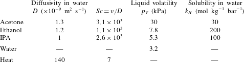
Properties of the substances used for the
 $\unicode[STIX]{x1D70E}$
-perturbation, given at
 $25\,^{\circ }\text{C}$
: diffusion coefficient in water
 $D$
, Schmidt number, vapour pressure
 $p_{V}$
and Henry’s law constant
 $k_{H}$
. Data from Pratt & Wakeham (Reference Pratt and Wakeham1975), Vargaftik, Vinogradov & Yargin (Reference Vargaftik, Vinogradov and Yargin1996), Lide (Reference Lide2010) and Linstrom & Mallard (Reference Linstrom and Mallard2017).
We alter the film surface properties from the outside in different ways, the objective being to perturb its surface tension locally in a controlled manner. This is achieved either by:
-
(i) projecting droplets of chemical substances different from water, but soluble in it like acetone, ethanol or isopropyl alcohol (IPA),
-
(ii) suspending at a controlled distance
 $\unicode[STIX]{x1D6FF}$
from the film a drop of known size
$2a$
, evaporating in the surrounding air and incorporating as dissolved gas in the film (see figure 2), a method initially mentioned by Maxwell (Reference Maxwell1875),
-
(iii) suspending a paper strip of known width, imbibed with the same volatile liquids,
-
(iv) approaching the tip of a soldering iron (typically
$T=300\,^{\circ }\text{C}$
), warming up the air around it and the film.


The perturbing chemical substances were chosen to be volatile and their vapour soluble in water (see their properties in table 1).
The distance
 $\unicode[STIX]{x1D6FF}$
separating the perturbation from the film, carefully measured, is varied from a centimetre, down to a fraction of a millimetre. The film is moving with velocity
 $U$
in a quiescent atmosphere: there forms an inevitable Blasius boundary layer around it. The latter sets a critical distance that grows with the distance
 $r$
to the jet impact as
 $\sqrt{\unicode[STIX]{x1D708}_{a}r/U}\sim 1~\text{mm}$
, with
 $\unicode[STIX]{x1D708}_{a}$
the air viscosity, and above which no effect could be seen and hardly measured: most of the observations were done with drops of pure substances evaporating in air, or the hot tip warming up the air, inside this boundary layer. Transfers across the boundary layer made the actual size of the perturbation
 $2a$
on the film slightly different from the typical size of the drop (typically 1 mm) or iron pan (typically 0.3 mm).
Surface tension dependences of isopropyl alcohol (IPA), ethanol (Vazquez, Alvarez & Navaza Reference Vazquez, Alvarez and Navaza1995) and acetone (Enders, Kahl & Winkelmann Reference Enders, Kahl and Winkelmann2007) solutions on their mole fraction in water. Dependence of water surface tension on temperature
 $T$
(Vargaftik, Volkov & Voljak Reference Vargaftik, Volkov and Voljak1983).

In all cases, the surface tension of the water film is lowered locally by a small amount
 $\unicode[STIX]{x0394}\unicode[STIX]{x1D70E}$
, compared to its base value
 $\unicode[STIX]{x1D70E}\approx 70~\text{mN}~\text{m}^{-1}$
. For instance, as can be seen from figure 3 collecting data of surface tension for different mixtures and temperatures (Vargaftik et al.
Reference Vargaftik, Volkov and Voljak1983; Vazquez et al.
Reference Vazquez, Alvarez and Navaza1995; Enders et al.
Reference Enders, Kahl and Winkelmann2007), decreasing by
 $1~\text{mN}~\text{m}^{-1}$
the surface tension of water implies warming up the liquid by
 $5\,^{\circ }\text{C}$
, or diluting it with traces of ethanol. It will be seen that, as small as they may seem to be, these local changes of the water composition have dramatic consequences on the film stability. Occasionally, we produced an ethanol film by the same method as the one described in § 2.1, which we perturbed by approaching a water droplet. In that case, the surface tension of the film was locally increased.
2.3 Imaging
The liquid film is stationary; it is perturbed either in a stationary fashion by altering locally its environment through the vapour composition (temperature) field introduced by a steady evaporating drop (hot source), or the perturbation is itself transient when a droplet is projected on the film. Still pictures were used to measure the perturbed film thickness fields, and high-speed imaging was useful for documenting the transients. Two main visualisation techniques were used, as detailed below.
2.3.1 Interferometry
In a first configuration, the liquid film is horizontal and lit by a monochromatic (
 $\unicode[STIX]{x1D706}=589~\text{nm}$
) low-pressure sodium lamp placed above, with an inclination angle of approximately
 $i\approx 45^{\circ }$
(figure 4
a). The reflected interference pattern is a series of stripes, each tracing a given film thickness (figure 5
a). The film thickness increment
 $\unicode[STIX]{x0394}h$
between two adjacent bright or dark fringes is
 $\unicode[STIX]{x0394}h=\unicode[STIX]{x1D706}/(2n\cos i_{r})$
, with
 $n$
the refractive index of the liquid and
 $i_{r}$
the refracted angle in the liquid (Isenberg Reference Isenberg1992). The slow
 $1/r$
film thickness decrease in (2.3) can be measured this way (Clanet & Villermaux Reference Clanet and Villermaux2002). Here, it is used to set an absolute reference from which the relative thickness is computed sequentially from one fringe to another (figure 5
b). In this way, following distorted fringes, the whole film thickness field may be interpolated. With water we have
 $\unicode[STIX]{x0394}h\approx 0.25~\unicode[STIX]{x03BC}\text{m}$
, so this quantitative technique, of which we will make extensive use in § 4, is very sensitive. With a typical image resolution of a few tens of pixels per millimetre, the maximal measurable thickness gradient between two distinguishable consecutive fringes is of the order of
 $\unicode[STIX]{x2202}_{x}h\sim 10^{-3}$
.
Visualisation techniques. (a) Interferometry: a sodium vapour lamp imprints stripes on the sheet. Two consecutive fringes are separated by a constant thickness jump
 $\unicode[STIX]{x0394}h=\unicode[STIX]{x1D706}/2n\cos i_{r}$
, with
 $i_{r}$
the refracted angle inside the sheet. (b) Schlieren: modulations of the thickness of the sheet, located in the plane of observation, deviate parallel light as would optical lenses.

Thickness measurement technique. (a) Typical interferometric picture. Each dark fringe is a line of iso-thickness, separating from the following by a constant
 $\unicode[STIX]{x0394}h\approx 0.25~\unicode[STIX]{x03BC}\text{m}$
. A reference is made where the film is unperturbed. (b) Iso-thickness ridges are plotted in three dimensions.

2.3.2 Schlieren
In a second configuration, the liquid film is formed in the vertical plane, and observed through a schlieren apparatus consisting of an arrangement of collimating lenses and pinholes (figure 4 b). Like the interferometry imaging technique described above, this technique does not give direct access to absolute measurements of the film thickness. It is, however, extremely sensitive to thickness modulations, since any curvature on the film plane acts as a lens, deflecting the light rays and thus producing either darker or brighter regions through the visualisation pinhole. The method singles out thickness gradients (Settles Reference Settles2001), and is useful at documenting, qualitatively, the dynamics of the transients (figures 7 and 8).
2.4 Qualitative observations
(a) Water or (b) ethanol droplet (
 $200~\unicode[STIX]{x03BC}\text{m}$
in diameter) falling on a moving water film (
 $U=3.5~\text{m}~\text{s}^{-1}$
) with thickness
 $h=18~\unicode[STIX]{x03BC}\text{m}$
. Pictures are 3.3 mm wide, recorded every
 $\unicode[STIX]{x0394}t=250~\unicode[STIX]{x03BC}\text{s}$
. (a) The water droplet rebounds, when (b) the ethanol droplet pierces the film. (c) Ethanol droplet (
 $150~\unicode[STIX]{x03BC}\text{m}$
in diameter) falling on a static soap film with thickness
 $h=5~\unicode[STIX]{x03BC}\text{m}$
, and rebounding. Pictures are 1.1 mm wide, recorded every
 $\unicode[STIX]{x0394}t=1~\text{ms}$
.

(a) Water droplet falling on a moving water film (
 $U=3.8~\text{m}~\text{s}^{-1}$
) with thickness
 $h=14~\unicode[STIX]{x03BC}\text{m}$
, and generating capillary waves. Pictures are 3.6 mm wide, recorded every
 $700~\unicode[STIX]{x03BC}\text{s}$
. (b) Ethanol droplet falling on a moving water film (
 $U=3.9~\text{m}~\text{s}^{-1}$
) with thickness
 $h=13~\unicode[STIX]{x03BC}\text{m}$
, and piercing it. Pictures are 5.8 mm wide, recorded every
 $500~\unicode[STIX]{x03BC}\text{s}$
.

Ethanol droplets approaching a
 $10~\unicode[STIX]{x03BC}\text{m}$
thick film falling downwards (
 $U=4.7~\text{m}~\text{s}^{-1}$
). (a) Pictures are 12 mm wide, recorded every
 $\unicode[STIX]{x0394}t=4~\text{ms}$
. Note the uneven hole opening shape after the droplet pierces the film. (b) Pictures are 9.3 mm wide,
 $\unicode[STIX]{x0394}t=2~\text{ms}$
. The tiny droplet rebounds on the film and modifies the thickness field, but does not puncture it (see also figure 1).

We illustrate the extreme sensitivity of liquid films to a variation of the chemical composition of their immediate surface environment.
When a water droplet
 $200~\unicode[STIX]{x03BC}\text{m}$
in diameter is slowly deposited on a water film
 $18~\unicode[STIX]{x03BC}\text{m}$
thick running at a few metres per second, it rebounds off it, slightly perturbing the film thickness field in a wake of capillary waves, which will soon damp, leaving the film intact (figure 6
a). On the other hand, if the exact same experiment is made using an ethanol droplet instead, then the fate of the film changes drastically (figure 6
b). Before the droplet has hit the film, the film thickness just below the droplet and its wake thins rapidly, leading to its irreversible puncture.
The same kind of observation is made using a schlieren type of visualisation (figure 7). While a water drop on a water film produces an impulse response type of capillary waves pattern before coalescing in it with no other consequence, an ethanol droplet moves the interstitial liquid in the film violently outward, digging it down to puncture. When the film is armoured with surfactant molecules (a commercial mixture of non-ionic and anionic molecules, by Dreft, Procter & Gamble), however, an ethanol droplet impacting on it rebounds (figure 6 c), with no puncture. The layer of surfactants has prevented the onset of an irreversible outward flow and subsequent film rupture observed in figures 6(b) and 7(b).
These observations, which are reminiscent of those made by Thoroddsen, Etoh & Takehara (Reference Thoroddsen, Etoh and Takehara2006) in a different but related context, also reveal that the ethanol droplet and the liquid film are in interaction, through the ethanol vapour field surrounding the volatile droplet before the droplet has contacted the film (figure 8 a). The strongly dissymmetrical shape of the opened hole after puncture demonstrates a posteriori that the film had already been dug in the wake of the droplet (the thinner the film, the faster the rim velocity). Thus, the minute quantities of ethanol which have evaporated from the droplet, have been mixed in the boundary layer at the surface of the running film, and have finally been incorporated at the surface of the liquid, are enough to produce a major and catastrophic change of the film thickness field. This suggests that a strong amplification mechanism is at play to move the interstitial liquid once its surface has been contaminated.
That mechanism has, nevertheless, a threshold. Figure 8(b) shows that the interaction of an ethanol droplet rebounding on a water film may not lead to film puncture if the droplet is too small, and the rebound time too short. The film thickness field is perturbed in the wake of the droplet, but is restored to a flat shape after rebound. This fact also suggests that a minimal quantity of ethanol should be incorporated in the liquid and/or that it should be deposited on a sufficiently large spot to trigger the amplification mechanism.
3 A mechanism
In order to make sense of the observations above, we first examine a simple argument, whose relevance will be investigated more closely on hand of precise experiments in § 4. We study a one-dimensional model of film dynamics for which the driving force is a gradient of concentration
 $c(x,t)$
of pollutant, translating in a gradient of surface tension by a linear transformation which suits to diluted traces of pollution (see figure 3):
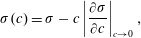 $$\begin{eqnarray}\displaystyle \unicode[STIX]{x1D70E}(c)=\unicode[STIX]{x1D70E}-c\left|\frac{\unicode[STIX]{x2202}\unicode[STIX]{x1D70E}}{\unicode[STIX]{x2202}c}\right|_{c\rightarrow 0}, & & \displaystyle\end{eqnarray}$$
with
 $\unicode[STIX]{x1D70E}$
the surface tension of the clean film. The interstitial liquid with velocity
 $\boldsymbol{u}=\{u_{x},u_{z}\}$
is set into a motion triggered by the Marangoni stress communicated across the film depth
 $h$
by liquid viscosity
 $\unicode[STIX]{x1D702}$
as
 $\unicode[STIX]{x2202}_{x}\unicode[STIX]{x1D70E}=\unicode[STIX]{x1D702}\unicode[STIX]{x2202}_{z}u_{x}$
, giving rise to a depth averaged velocity
 $v(x,t)=\int _{0}^{h}u_{x}\,\text{d}z/h$
describing a plug flow along the film provided
 $|v/h|\gg |\unicode[STIX]{x2202}_{x}\unicode[STIX]{x1D70E}/\unicode[STIX]{x1D702}|$
.
A one-dimensional model disregarding the phenomena occurring in the depth of the film will hold for times larger than the diffusion time of mass across the film
 $h^{2}/D$
for the two interfaces of the film to be equally affected by the concentration of pollutants, and larger than the diffusion time of vorticity
 $h^{2}/\unicode[STIX]{x1D708}$
for the superficial stress to be communicated to the entire film depth (
 $\unicode[STIX]{x1D708}=\unicode[STIX]{x1D702}/\unicode[STIX]{x1D70C}$
, with
 $\unicode[STIX]{x1D70C}$
the liquid density). Given the Schmidt number of ethanol in water,
 $Sc=\unicode[STIX]{x1D708}/D=O(10^{3})$
, the second condition is easily met when the first is (figure 9
a).
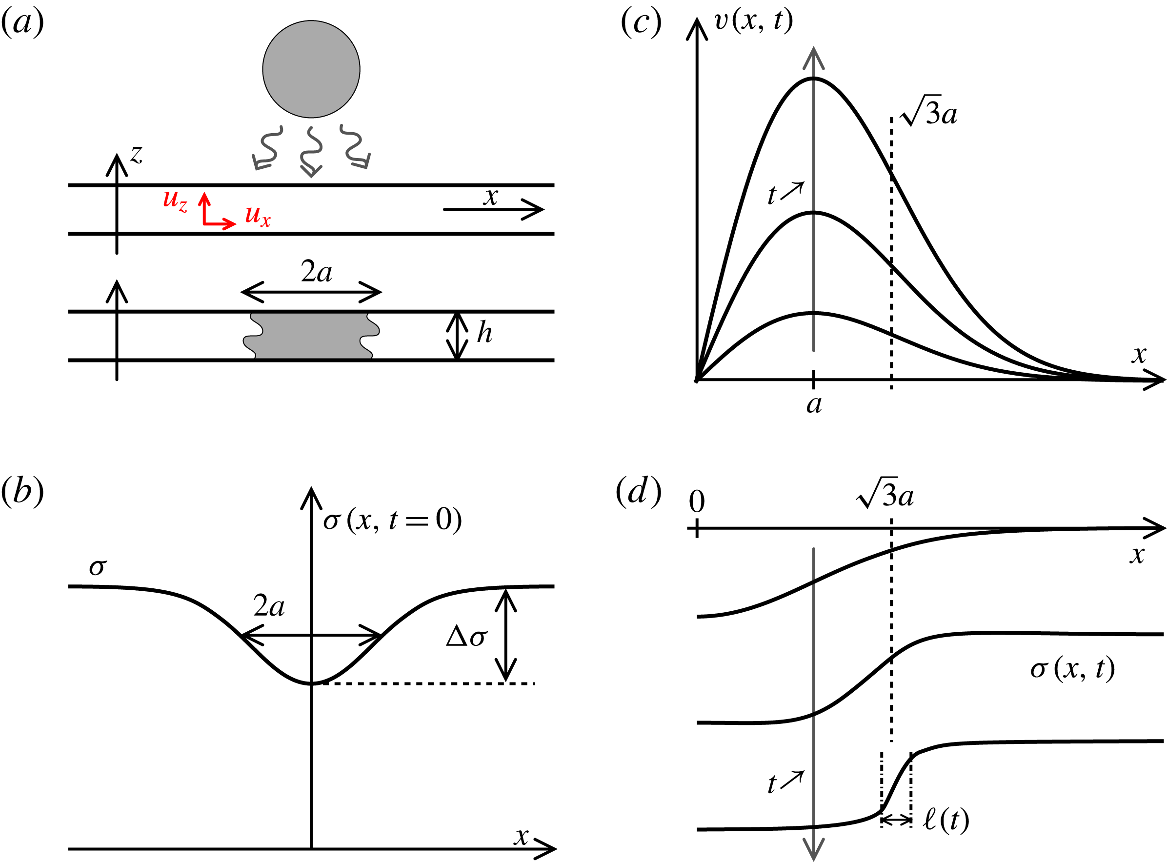
Sketch of the mechanism. (a) A liquid film with thickness
 $h$
being contaminated over a size
 $2a$
. (b) Initial profile of the liquid surface tension. (c) Induced displacement field
 $v(x,t)$
along the film for increasing times
 $t$
. (d) Surface tension profiles for increasing times illustrating the existence of a plateau at
 $\unicode[STIX]{x1D70E}-\unicode[STIX]{x0394}\unicode[STIX]{x1D70E}$
around
 $x=0$
, and a steepening front around
 $x=a\sqrt{3}$
of decreasing width
 $\ell (t)$
.
In that idealised limit, the transport of the pollutant concentration along the film results from both substrate motion and molecular diffusion with flux
 $j=-D\unicode[STIX]{x2202}_{x}c$
. A detailed balance provides
 $$\begin{eqnarray}\displaystyle & \displaystyle \unicode[STIX]{x2202}_{t}c+v\unicode[STIX]{x2202}_{x}c=-\unicode[STIX]{x2202}_{x}\,j-j\frac{\unicode[STIX]{x2202}_{x}h}{h}, & \displaystyle\end{eqnarray}$$
 $$\begin{eqnarray}\displaystyle & \displaystyle j=-D\unicode[STIX]{x2202}_{x}c, & \displaystyle\end{eqnarray}$$
while mass conservation of the substrate, in the same one-dimensional approximation, is given by
 $$\begin{eqnarray}\displaystyle \unicode[STIX]{x2202}_{t}h+\unicode[STIX]{x2202}_{x}(hv)=0. & & \displaystyle\end{eqnarray}$$
The flow will result from the contamination of the film interface over a size
 $2a$
, typically larger than the film thickness
 $h$
. We anticipate an induced flow with velocity
 $|v|$
such that
 $|v|a/\unicode[STIX]{x1D708}\gg 1$
. In other words, if viscosity dominates the transfer of momentum across the film, it is negligible for the motion along the film. The momentum balance is thus given by
 $$\begin{eqnarray}\displaystyle \unicode[STIX]{x2202}_{t}v+v\unicode[STIX]{x2202}_{x}v=\frac{2}{\unicode[STIX]{x1D70C}h}\unicode[STIX]{x2202}_{x}\unicode[STIX]{x1D70E}-\frac{1}{\unicode[STIX]{x1D70C}}\unicode[STIX]{x2202}_{x}\{\unicode[STIX]{x1D70E}{\mathcal{K}}\}, & & \displaystyle\end{eqnarray}$$
where the factor 2 stands for the two sides of the film, and
 ${\mathcal{K}}$
is the film thickness curvature.
In order to reach a meaningful solution to this model through a tractable analysis, we make further simplifications. We study the dynamics of the film from its initial immobility, and therefore
 $|v\unicode[STIX]{x2202}_{x}v|\ll |\unicode[STIX]{x2202}_{t}v|$
. The film is initially smooth so that
 $|\unicode[STIX]{x2202}_{x}h|\rightarrow 0$
, and we concentrate on films which are planar but dirty so that the Laplace term
 $h\unicode[STIX]{x2202}_{x}\{\unicode[STIX]{x1D70E}{\mathcal{K}}\}$
is subdominant to the Marangoni stress
 $\unicode[STIX]{x2202}_{x}\unicode[STIX]{x1D70E}$
in (3.5). This being posed, making use of (3.1), (3.2) and (3.5) provides
 $$\begin{eqnarray}\displaystyle & \displaystyle \unicode[STIX]{x2202}_{t}v=\frac{2}{\unicode[STIX]{x1D70C}h}\unicode[STIX]{x2202}_{x}\unicode[STIX]{x1D70E} & \displaystyle\end{eqnarray}$$
 $$\begin{eqnarray}\displaystyle & \unicode[STIX]{x2202}_{t}\unicode[STIX]{x1D70E}+v\unicode[STIX]{x2202}_{x}\unicode[STIX]{x1D70E}=D\unicode[STIX]{x2202}_{x}^{2}\unicode[STIX]{x1D70E} & \displaystyle\end{eqnarray}$$
describing, together with (3.4), how the film dynamics is coupled to the pollutant concentration field (of which the
 $\unicode[STIX]{x1D70E}$
-field is an inverted image, from (3.1)). Surface tension (concentration) diffuses along the film on a substrate whose velocity
 $v$
varies according to its gradient. If it happens that the induced flow reinforces the surface tension gradient, a dramatic dynamics may result.
3.1 A spot of dirt
The examples we have listed in §§ 2.2 and 2.4 all involve a perturbation introduced locally on the surface of the film which is made ‘dirty’ over a given size
 $2a$
where the liquid surface tension is lowered. We thus represent the initial spot of dirt by a smooth bell-shaped deficit of surface tension with intensity
 $\unicode[STIX]{x0394}\unicode[STIX]{x1D70E}$
and width
 $a$
by (figure 9
b)
 $$\begin{eqnarray}\displaystyle & \displaystyle \unicode[STIX]{x1D70E}(x,t=0)=\unicode[STIX]{x1D70E}-\unicode[STIX]{x0394}\unicode[STIX]{x1D70E}\text{e}^{-(x^{2}/2a^{2})}, & \displaystyle\end{eqnarray}$$
 $$\begin{eqnarray}\displaystyle & \displaystyle \text{so that}\quad \unicode[STIX]{x2202}_{x}\unicode[STIX]{x1D70E}|_{t=0}=\frac{\unicode[STIX]{x0394}\unicode[STIX]{x1D70E}}{a^{2}}x\text{e}^{-(x^{2}/2a^{2})}. & \displaystyle\end{eqnarray}$$
This initial surface tension gradient accelerates the interstitial fluid according to (3.6) so that the initial motion of the film has velocity (on the
 $x>0$
side, see figure 9
c)
 $$\begin{eqnarray}\displaystyle v(x,t)\sim \frac{t\,x}{\unicode[STIX]{x1D70F}_{0}^{2}}\text{e}^{-(x^{2}/2a^{2})}, & & \displaystyle\end{eqnarray}$$
where
 $\unicode[STIX]{x1D70F}_{0}$
is the characteristic time of the motion
 $$\begin{eqnarray}\displaystyle \unicode[STIX]{x1D70F}_{0}=\sqrt{\frac{\unicode[STIX]{x1D70C}ha^{2}}{\unicode[STIX]{x0394}\unicode[STIX]{x1D70E}}}, & & \displaystyle\end{eqnarray}$$
with
 $h$
the initial film thickness. The velocity (3.10) increases from
 $x=0$
, then reaches a maximum, and decays far from the spot for
 $x\gg a$
. Fluid particles at the centre of the spot are stretched and moved towards the spot periphery where they are stuck and compressed in the region where the velocity gradient is negative. The analysis of the
 $\unicode[STIX]{x1D70E}$
-field dynamics in that region is worthy of interest since it explains why and when the initial rearrangements along the film in (3.10) may amplify or relax.
An obvious candidate for relaxation is the diffusive smearing of the contaminant. The typical time it takes for the dirty spot to diffuse over its initial size is
 $a^{2}/D$
, and if it does so within less than
 $\unicode[STIX]{x1D70F}_{0}$
, the rearrangements described above will not have time to occur before the film has come back to surface homogeneity. Another way of expressing the same condition is to write it in terms of velocities, comparing the diffusion velocity
 $D/a$
with the Taylor–Culick speed based on the surface tension deficit
 $\sqrt{\unicode[STIX]{x0394}\unicode[STIX]{x1D70E}/\unicode[STIX]{x1D70C}h}$
. When the latter is larger than the former, that is, when the Péclet number
 $$\begin{eqnarray}Pe=\frac{a^{2}}{D\unicode[STIX]{x1D70F}_{0}}\end{eqnarray}$$
is larger than unity, rearrangements can occur. We thus examine below the interplay between dirt diffusion along the film and the displacement field induced by its initial inhomogeneity.
3.2 Mixing analogy
We call
 $\unicode[STIX]{x1D6FE}$
the maximal rate of compression along the film obtained in
 $x=a\sqrt{3}$
,
 $$\begin{eqnarray}\displaystyle \unicode[STIX]{x1D6FE}=\max (-\unicode[STIX]{x2202}_{x}v)\sim \frac{t}{\unicode[STIX]{x1D70F}_{0}^{2}}, & & \displaystyle\end{eqnarray}$$
and expand the negatively sloped velocity
 $v(x,t)=v(a\sqrt{3},t)-\unicode[STIX]{x1D6FE}\,\tilde{x}$
about this point, with
 $\tilde{x}=x-a\sqrt{3}$
. In that shifted frame, the transport equation of surface tension (3.7) has the characteristic form of a diffusion problem on a deformed substrate well known in the scalar mixing context (Ranz Reference Ranz1979; Villermaux & Duplat Reference Villermaux and Duplat2003; Villermaux Reference Villermaux2012),
 $$\begin{eqnarray}\displaystyle \unicode[STIX]{x2202}_{t}\unicode[STIX]{x1D70E}-\unicode[STIX]{x1D6FE}\tilde{x}\unicode[STIX]{x2202}_{\tilde{x}}\unicode[STIX]{x1D70E}=D\unicode[STIX]{x2202}_{\tilde{x}}^{2}\unicode[STIX]{x1D70E}, & & \displaystyle\end{eqnarray}$$
expressing how substrate compression and diffusive broadening compete. A suitable transformation of space and time maps (3.14) onto a pure diffusion equation. Let
 $s(t)$
be the distance between two material points initially distant from
 $a$
in that region of the substrate; then
 $$\begin{eqnarray}\displaystyle \frac{{\dot{s}}}{s}=-\unicode[STIX]{x1D6FE},\quad \text{or}\quad s(t)=a\text{e}^{-(t^{2}/2\unicode[STIX]{x1D70F}_{0}^{2})}, & & \displaystyle\end{eqnarray}$$
and further defining (Ranz Reference Ranz1979)
 $$\begin{eqnarray}\displaystyle \unicode[STIX]{x1D709}=\frac{\tilde{x}}{s(t)}\quad \text{and}\quad \unicode[STIX]{x1D70F} & = & \displaystyle D\int _{0}^{t}\frac{dt^{\prime }}{s(t^{\prime })^{2}}\end{eqnarray}$$
 $$\begin{eqnarray}\displaystyle & = & \displaystyle \frac{1}{2Pe}\int _{0}^{(t/\unicode[STIX]{x1D70F}_{0})^{2}}\frac{\text{e}^{z}}{\sqrt{z}}\,\text{d}z,\end{eqnarray}$$
we have
 $$\begin{eqnarray}\displaystyle \unicode[STIX]{x2202}_{\unicode[STIX]{x1D70F}}\unicode[STIX]{x1D70E}=\unicode[STIX]{x2202}_{\unicode[STIX]{x1D709}}^{2}\unicode[STIX]{x1D70E} & & \displaystyle\end{eqnarray}$$
whose solutions are known for any initial spatial profile of
 $\unicode[STIX]{x1D70E}$
. In particular, molecular diffusion alters the distribution of the
 $\unicode[STIX]{x1D70E}$
levels for times
 $\unicode[STIX]{x1D70F}$
larger than unity (Villermaux & Duplat Reference Villermaux and Duplat2003). If the Péclet number is small, that condition will be reached while
 $\unicode[STIX]{x1D70F}$
essentially behaves like the normal time
 $t$
as in a pure diffusion process:
 $$\begin{eqnarray}\displaystyle \unicode[STIX]{x1D70F}\xrightarrow[{}]{Pe\ll 1}\frac{Dt}{a^{2}}. & & \displaystyle\end{eqnarray}$$
In contrast, if the Péclet number is large, integrating
 $\unicode[STIX]{x1D70F}$
in (3.17) by parts shows that it varies extremely fast with time as
 $$\begin{eqnarray}\displaystyle \unicode[STIX]{x1D70F}\xrightarrow[{}]{Pe\gg 1}\frac{1}{2Pe}\frac{\text{e}^{(t/\unicode[STIX]{x1D70F}_{0})^{2}}}{t/\unicode[STIX]{x1D70F}_{0}} & & \displaystyle\end{eqnarray}$$
in its route towards the condition
 $\unicode[STIX]{x1D70F}(t_{s})=O(1)$
which defines the mixing time
 $t_{s}$
. That time is simply the diffusion time
 $a^{2}/D$
for
 $Pe\ll 1$
, and is
 $$\begin{eqnarray}\displaystyle t_{s}\sim \unicode[STIX]{x1D70F}_{0}\sqrt{\ln Pe}, & & \displaystyle\end{eqnarray}$$
essentially given by the kinematic time
 $\unicode[STIX]{x1D70F}_{0}$
, very weakly dependent on molecular diffusion for
 $Pe\gg 1$
.
3.3 Consequences
The schematic scenario depicted above has an interesting consistency with some of the observations reported in § 2.4, and provides additional predictions.
First, this mechanism accounts for the existence of a threshold. If the spot is too small (small
 $a$
), or too faint (weak
 $\unicode[STIX]{x0394}\unicode[STIX]{x1D70E}$
and hence large
 $\unicode[STIX]{x1D70F}_{0}$
), the Péclet number will be smaller than one, and the perturbation of surface tension will simply vanish by molecular diffusion before the film has appreciably moved. This is consistent with the comparison made in figure 8 showing that a tiny droplet of ethanol rebounding at the film surface does not alter it much, while a similar droplet coalescing with the film (thus producing a stronger
 $\unicode[STIX]{x0394}\unicode[STIX]{x1D70E}$
, hence a smaller
 $\unicode[STIX]{x1D70F}_{0}$
and therefore a larger
 $Pe$
) leads to rupture.
Second, this mechanism describes the morphology of the depleted region of the film before rupture. For
 $Pe\gg 1$
, the motion along the film caused by an initial surface tension gradient reinforces that gradient in a self-amplified fashion. The amplification is so strong (the distance between kinematic markers in (3.15) shrinks faster than exponentially) that even after the mixing time, molecular diffusion does not damp it. The width of the surface tension gradient in the compression zone
 $\ell (t)$
, a generalised Batchelor scale (Batchelor Reference Batchelor1959; de Rivas & Villermaux Reference de Rivas and Villermaux2016), is such that (see (3.15) and (3.20))
 $$\begin{eqnarray}\displaystyle & \displaystyle \ell (t)\sim s(t)\sqrt{\unicode[STIX]{x1D70F}}, & \displaystyle\end{eqnarray}$$
 $$\begin{eqnarray}\displaystyle & \displaystyle \sim \frac{a}{\sqrt{Pe}}\sqrt{\frac{\unicode[STIX]{x1D70F}_{0}}{t}}=\unicode[STIX]{x1D70F}_{0}\sqrt{\frac{D}{t}}\quad \text{for }Pe\gg 1, & \displaystyle\end{eqnarray}$$
thus building a steepening front at the periphery of the spot (figure 9
d), with gradient of the order of
 $\unicode[STIX]{x0394}\unicode[STIX]{x1D70E}/\ell (t)$
.
(a) Wave pattern (and film rupture) generated by a droplet of ethanol (
 $a=100~\unicode[STIX]{x03BC}\text{m}$
) landing on a thick water film
 $h=250~\unicode[STIX]{x03BC}\text{m}$
. Pictures are 8.6 mm wide, recorded every
 $800~\unicode[STIX]{x03BC}\text{s}$
, reading from left to right, top to bottom. (b) Wave crests are tracked along time and their location
 $x_{crests}$
is plotted in logarithmic scale.

At the centre of the spot close to
 $x=0$
, the situation is exactly the opposite. There, the velocity gradient
 $\unicode[STIX]{x2202}_{x}v$
in (3.10) is positive, with the same intensity
 $t/\unicode[STIX]{x1D70F}_{0}^{2}$
in absolute value than in the compressive region, but is now smoothing the surface tension gradient (the equation describing the phenomenon is identical to (3.14), with a plus sign in front of the convection term). Similar lines as above show that
 $\unicode[STIX]{x1D70F}$
now saturates as
 $\unicode[STIX]{x1D70F}\rightarrow 1/Pe$
for
 $Pe\gg 1$
, and that the surface tension profile is a plateau with height
 $\unicode[STIX]{x1D70E}-\unicode[STIX]{x0394}\unicode[STIX]{x1D70E}$
. The surface tension gradient is expelled at the periphery of the blob by a flow pushing the fluid particles outwards up to the periphery of the spot, where they accumulate in a bump. That accumulation causes the radiation of waves in the rest of the film (
 $x>a$
), which are convincingly of the varicose type (Taylor Reference Taylor1959a
). The wave (with pulsation
 $\unicode[STIX]{x1D714}$
and wavenumber
 $k$
) crest displacements
 $x_{crests}$
in time
 $t$
in the growing bump have a self-similar pattern in
 $x^{2}/t$
, consistent with their dispersion equation
 $\unicode[STIX]{x1D714}^{2}=(\unicode[STIX]{x1D70E}h/\unicode[STIX]{x1D70C})k^{4}$
in the long wave limit
 $kh\ll 1$
(see figure 10 and Duchemin et al.
Reference Duchemin, Le Dizès, Vincent and Villermaux2015).
Finally, the spot concomitantly depletes at its centre, digging the film down to the cancelling of its thickness. Close to the spot centre where
 $\unicode[STIX]{x2202}_{x}h=0$
by symmetry, equations (3.4) and (3.10) provide
 $$\begin{eqnarray}\displaystyle \frac{{\dot{h}}}{h}=-\unicode[STIX]{x2202}_{x}v|_{x=0}\sim -\frac{t}{\unicode[STIX]{x1D70F}_{0}(h)^{2}}. & & \displaystyle\end{eqnarray}$$
If one naively retains the current value of
 $h$
in
 $\unicode[STIX]{x1D70F}_{0}(h)$
in order to extend the prediction of this short-time mechanism to subsequent instants of time, one anticipates from (3.24) that the film thickness goes to zero in a finite time, of the order of
 $\unicode[STIX]{x1D70F}_{0}$
based on the initial film thickness given in (3.11): the film ruptures. The case of a unilateral front is presented in appendix A.
However, the present mechanism predicts only an amplification of the gradient of
 $\unicode[STIX]{x1D70E}$
through the action of a displacement field caused by its initial spatial inhomogeneity. We have not described the retroaction of the modified
 $\unicode[STIX]{x1D70E}$
-field on the displacement field itself which, since the effect reinforces the cause (the steepness of the
 $\unicode[STIX]{x1D70E}$
-field), will unavoidably lead to rapid film thinning, even before the ultimate regime where (3.23) holds is reached. It is in that sense that the mechanism we have described is ‘self-sustained’ (see also the related discussion in Burton & Taborek Reference Burton and Taborek2007).
3.4 In two dimensions
Films in nature are planar, and one may wonder how the scenario analysed above is altered when the perturbation is no longer along a segment but has a radius
 $a$
, producing a radial flow expanding in two dimensions, as for all the examples we have shown in § 2.4. Within the same approximation as in (3.7), the two-dimensional transport equation for surface tension is
 $$\begin{eqnarray}\displaystyle \unicode[STIX]{x2202}_{t}\unicode[STIX]{x1D70E}+v\unicode[STIX]{x2202}_{r}\unicode[STIX]{x1D70E}=\frac{D}{r}\unicode[STIX]{x2202}_{r}(r\unicode[STIX]{x2202}_{r}\unicode[STIX]{x1D70E}) & & \displaystyle\end{eqnarray}$$
for an axisymmetric spot
 $\unicode[STIX]{x1D70E}(r,t)$
evolving through a radial flow
 $v(r,t)$
depending on the radial coordinate
 $r$
. The phenomenology is qualitatively identical to the one-dimensional case, and presents a compressive region at the periphery of the spot in
 $r_{c}=a\sqrt{3}$
where we expand the velocity as
 $v(r,t)=v(r_{c},t)-\unicode[STIX]{x1D6FE}\tilde{r}$
with
 $\tilde{r}=r-r_{c}$
. The equivalent of (3.14) now reads
 $$\begin{eqnarray}\displaystyle \unicode[STIX]{x2202}_{t}\unicode[STIX]{x1D70E}-\unicode[STIX]{x1D6FE}\tilde{r}\unicode[STIX]{x2202}_{\tilde{r}}\unicode[STIX]{x1D70E}=\frac{D}{\tilde{r}+r_{c}}\unicode[STIX]{x2202}_{\tilde{r}}\{(\tilde{r}+r_{c})\unicode[STIX]{x2202}_{\tilde{r}}\unicode[STIX]{x1D70E}\}. & & \displaystyle\end{eqnarray}$$
The width of the compression region shrinks, and the
 $\unicode[STIX]{x1D70E}$
-field varies essentially over a length scale
 $\ell (t)$
decreasing in time. The expansion leading to (3.26) is thus valid for excursions
 $r$
about
 $r_{c}$
small compared to
 $\ell (t)$
. Therefore,
 $|\tilde{r}|=O(\ell (t))$
at most and as soon as
 $\ell (t)/r_{c}<1$
, the two-dimensional problem (3.26) amounts to its one-dimensional version (3.14). Because the flow builds a thinning compressing front, the one-dimensional approximation is soon valid.
4 Detailed measurements
Having discussed a possible mechanism for the spontaneous dramatic thinning and puncture of dirty liquid films, we now investigate its relevance on hand of a controlled experiment, where all the transients can be measured and quantified.
4.1 Experiments on a Savart sheet
We use stationary, self-cleaned water films produced by a Savart sheet as described in § 2.1. The mechanism in § 3 relies on two physical quantities of interest, namely the time scale
 $\unicode[STIX]{x1D70F}_{0}$
and the Péclet number
 $Pe$
based on this time. For example, a spot of size
 $a=100~\unicode[STIX]{x03BC}\text{m}$
made up of dissolved ethanol (
 $D\sim 10^{-9}~\text{m}^{2}~\text{s}^{-1}$
) inducing an arbitrary surface tension deficit of
 $0.1~\text{mN}~\text{m}^{-1}$
on a water film (density
 $\unicode[STIX]{x1D70C}=10^{3}~\text{kg}~\text{m}^{-3}$
) with thickness
 $h=10~\unicode[STIX]{x03BC}\text{m}$
, will result in an instability time of order
 $\unicode[STIX]{x1D70F}_{0}\sim 1~\text{ms}$
(3.11) – a time scale comfortably larger than the time of vorticity transfer across the film
 $h^{2}/\unicode[STIX]{x1D708}\sim 10^{-1}~\text{ms}$
. The Péclet number will then be estimated at
 $Pe\sim 10^{4}\gg 1$
: clearly, molecular diffusion will not regularise this spot, and the self-amplified scenario in § 3 is likely to hold.
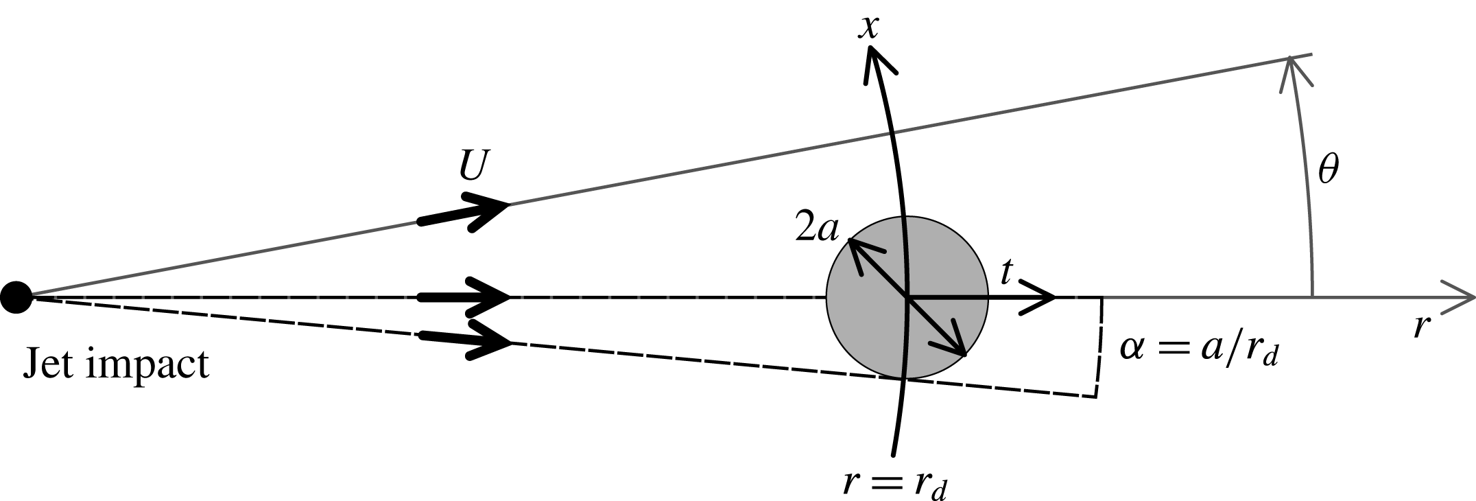
Geometrical transform of the natural
 $(\unicode[STIX]{x1D703},r)$
coordinates of the circular Savart sheet into
 $(x,t)$
, the coordinates of the mechanism.
In a Savart sheet, advection of the fluid particles at constant radial velocity
 $U$
(typically
 $U=3~\text{m}~\text{s}^{-1}$
) conveniently maps time onto a measurable distance since the surface tension perturbation is fixed in the laboratory frame. The disturbance with size
 $2a$
is introduced at the distance
 $r_{d}$
from the impact point, and because of the circular expansion of the sheet, an ingredient which does not modify the physical content of the problem, we will need a divergence angle
 $\unicode[STIX]{x1D6FC}=a/r_{d}$
(see figures 2 and 11). The spatial and temporal coordinates
 $(x,t)$
defined previously in § 3 are recovered from the ortho-radial and radial coordinates
 $(\unicode[STIX]{x1D703},r)$
used in the Savart sheet (figure 11) as
 $$\begin{eqnarray}\displaystyle & \displaystyle x=r\unicode[STIX]{x1D703}\simeq r_{d}\unicode[STIX]{x1D703}, & \displaystyle\end{eqnarray}$$
 $$\begin{eqnarray}\displaystyle & \displaystyle t=\frac{r-r_{d}}{U}. & \displaystyle\end{eqnarray}$$
In the frame of the laboratory, the flow in the sheet, whether or not it is disturbed, is stationary. The equations describing the motion of the film are thus adapted from § 3 in this particular diverging geometry. Under the same assumptions, substrate mass conservation must account for the undisturbed radial film thickness decrease in (2.3), a consequence of the base flow divergence, and we have
 $$\begin{eqnarray}\displaystyle U\unicode[STIX]{x2202}_{r}(hr)+\unicode[STIX]{x2202}_{\unicode[STIX]{x1D703}}(hv)=0, & & \displaystyle\end{eqnarray}$$
with
 $v$
the ortho-radial, depth averaged velocity, defined as in § 3. Equation (4.3) amounts to (3.4) at short distance (times)
 $\unicode[STIX]{x1D6FF}r=U\unicode[STIX]{x1D6FF}t$
after
 $r_{d}$
. The dynamics equation along the ortho-radial coordinate
 $\unicode[STIX]{x1D703}$
reads
 $$\begin{eqnarray}U\unicode[STIX]{x2202}_{r}(rv)=\frac{2}{\unicode[STIX]{x1D70C}h}\unicode[STIX]{x2202}_{\unicode[STIX]{x1D703}}\unicode[STIX]{x1D70E},\end{eqnarray}$$
which, again, restores (3.6) for small distances
 $\unicode[STIX]{x1D6FF}r$
after
 $r_{d}$
. Similarly to (3.7), the pollutant concentration (surface tension) transport along the sheet is described by
 $$\begin{eqnarray}\displaystyle U\unicode[STIX]{x2202}_{r}\unicode[STIX]{x1D70E}+\frac{v}{r}\unicode[STIX]{x2202}_{\unicode[STIX]{x1D703}}\unicode[STIX]{x1D70E}=\frac{D}{r^{2}}\unicode[STIX]{x2202}_{\unicode[STIX]{x1D703}}^{2}\unicode[STIX]{x1D70E}, & & \displaystyle\end{eqnarray}$$
which, as well, reduces to (3.7) for small
 $\unicode[STIX]{x1D6FF}r$
after
 $r_{d}$
. Therefore, close to the
 $\unicode[STIX]{x1D70E}$
-disturbance in
 $r=r_{d}$
, the one-dimensional description holds, whereas at larger distances (times), the transverse coordinate
 $x=r\unicode[STIX]{x1D703}$
cannot be approximated by
 $r_{d}\unicode[STIX]{x1D703}$
anymore. We thus formalise the problem in terms of angles, rather than distances, i.e. in terms of
 $\unicode[STIX]{x1D703}$
, whose reference scale is
 $\unicode[STIX]{x1D6FC}=a/r_{d}$
.
4.2 The spot of dirt and initial response
Velocity measurements of the interstitial flow. (a) Superposition of 500 images grabbed at 3 kHz. (b) Close-up view of the tracked particles in the correct coordinates system. Picture is 19 mm wide. (c) Transverse velocity
 $v$
as a function of the angle
 $\unicode[STIX]{x1D703}$
to the drop, averaged around four successive times (i.e. radii) from the drop location (for clarity, only positive angles are plotted). Acetone drop, water film (
 $U=2.2~\text{m}~\text{s}^{-1}$
,
 $Fr=50$
,
 $h=88~\unicode[STIX]{x03BC}\text{m}$
),
 $r_{d}=23~\text{mm}$
,
 $\unicode[STIX]{x1D6FC}=2.5^{\circ }$
,
 $\unicode[STIX]{x1D70F}_{0}=5.1~\text{ms}$
,
 $\unicode[STIX]{x0394}\unicode[STIX]{x1D70E}\simeq 3~\text{mN}~\text{m}^{-1}$
,
 $Pe=1.5\times 10^{5}$
. Inset: the amplitude
 $|v|$
in the expression
 $v=|v|\unicode[STIX]{x1D703}\exp (-\unicode[STIX]{x1D703}^{2}/2\unicode[STIX]{x1D6FC}^{2})$
(see (4.6)) is fitted to the experimental data and plotted versus time
 $t$
for the corresponding successive times. The time scale
 $\unicode[STIX]{x1D70F}_{0}$
reads directly from the slope
 $r_{d}/\unicode[STIX]{x1D70F}_{0}^{2}$
.

A disturbance of surface tension is applied to the clean film, according to the methods described in § 2.2. It behaves like a dirty spot of size
 $2a$
, modelled by a bell-shaped curve as in (3.9) at
 $r=r_{d}$
(i.e.
 $t=0$
). The short-time velocity field corresponds to the one in (3.10), written in terms of
 $\unicode[STIX]{x1D703}$
,
 $$\begin{eqnarray}\displaystyle v(\unicode[STIX]{x1D703},t)\sim \frac{tr_{d}}{\unicode[STIX]{x1D70F}_{0}^{2}}\unicode[STIX]{x1D703}\text{e}^{-(\unicode[STIX]{x1D703}^{2}/2\unicode[STIX]{x1D6FC}^{2})}, & & \displaystyle\end{eqnarray}$$
with
 $\unicode[STIX]{x1D70F}_{0}$
given by (3.11). Figure 12 shows the velocity measurements obtained from particles (
 $d_{p}=10~\unicode[STIX]{x03BC}\text{m}$
in diameter) introduced inside the water bulk prior to the formation of the sheet. Their displacement is observed by backlighting using a high-speed camera (figure 12
a). Particles were chosen so that their Stokes number
 $St=(d_{p}^{2}/\unicode[STIX]{x1D708})/\unicode[STIX]{x1D70F}_{0}$
, is at most about
 $10^{-1}$
so that they behave as passive tracers. Tracking a few hundreds of tracers along their trajectories gives access to time averaged velocity profiles, as a function of the angle
 $\unicode[STIX]{x1D703}$
(figure 12
b). The profile shape, shown for positive angles, indicates the presence of an interstitial velocity
 $v$
, removing the liquid out of the central zone where surface tension has been lowered. The outward velocity is of the order of a few
 $\text{cm}~\text{s}^{-1}$
, much smaller than the radial velocity
 $U$
, of the order of
 $\text{m}~\text{s}^{-1}$
. Fitting expression (4.6) to the experimental profiles shows fair agreement. Then, plotting the velocity amplitude versus time reveals the expected linear dependency, predicted in § 3. The slope
 $r_{d}/\unicode[STIX]{x1D70F}_{0}^{2}$
gives a direct measurement for
 $\unicode[STIX]{x1D70F}_{0}=5.1~\text{ms}$
. From (3.11), we estimate the initial surface tension gap
 $\unicode[STIX]{x0394}\unicode[STIX]{x1D70E}\simeq 3~\text{mN}~\text{m}^{-1}$
, a small surface tension deficit relative to the surface tension of the water liquid film (
 $\unicode[STIX]{x1D70E}\approx 70~\text{mN}~\text{m}^{-1}$
).
Film thickness. (a) Interpolated thickness field. (b) Transverse thickness profiles for different times (distances) after the perturbation. Experimental data (points) are plotted along with the prediction in (4.7) (solid line) with
 $r_{d}=3.3~\text{cm}$
, with
 $\unicode[STIX]{x1D6FC}=0.8\pm 0.1^{\circ }$
and
 $\unicode[STIX]{x1D70F}_{0}=6.5~\text{ms}$
, giving
 $Pe=3\times 10^{4}$
. Ethanol drop, water film,
 $U=3.2~\text{m}~\text{s}^{-1}$
,
 $h=34~\unicode[STIX]{x03BC}\text{m}$
.
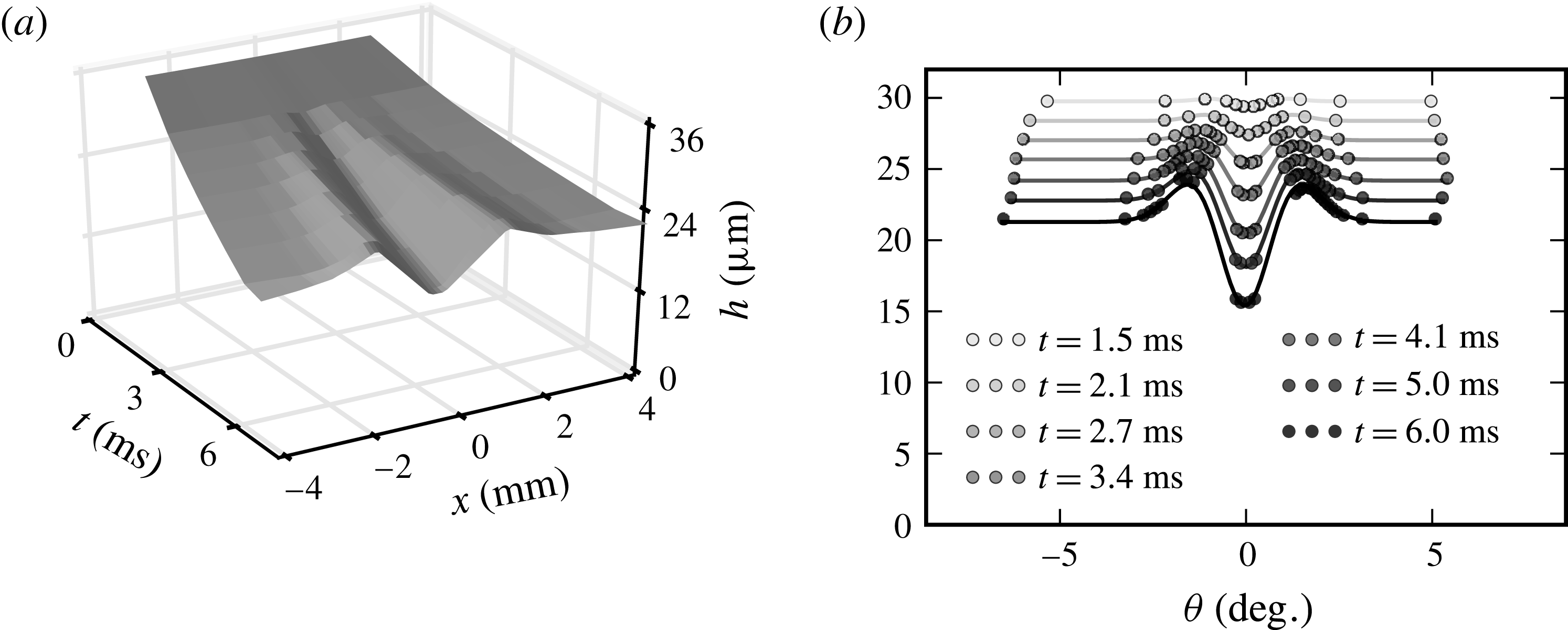
The short-time behaviour of the surface thickness is derived from (3.4) as
 $$\begin{eqnarray}\frac{h(\unicode[STIX]{x1D703},t)}{h}=1-\frac{t^{2}}{2\unicode[STIX]{x1D70F}_{0}^{2}}\left(1-\frac{\unicode[STIX]{x1D703}^{2}}{\unicode[STIX]{x1D6FC}^{2}}\right)\text{e}^{-(\unicode[STIX]{x1D703}^{2}/2\unicode[STIX]{x1D6FC}^{2})}\end{eqnarray}$$
and is compared to the interferometric measurements of § 2 in figure 13, with
 $\unicode[STIX]{x1D6FC}$
and
 $\unicode[STIX]{x1D70F}_{0}$
as fitting parameters. Because of the mean radial divergence of the sheet, the thickness profiles are shifted, in the mean, towards lower values for larger distances (times) from the pollutant source (figure 13
b), while concomitantly a central depletion bordered by bumps grows in amplitude, digging the film. From the fitted time
 $\unicode[STIX]{x1D70F}_{0}=6.5~\text{ms}$
and
 $a=0.5~\text{mm}$
and the measured film thickness at the location of the perturbation
 $h=34~\unicode[STIX]{x03BC}\text{m}$
corresponding to the perturbation shown in figure 13, we anticipate that
 $\unicode[STIX]{x0394}\unicode[STIX]{x1D70E}\approx 0.1~\text{mN}~\text{m}^{-1}$
, an even smaller fraction indeed of the bare liquid film surface tension, than with the perturbation corresponding to figure 12.
The transverse flow (figure 12) and consecutive local film thinning (figure 13) evidenced here and successfully comparing to the theoretical predictions at short times thus support the early dynamics mechanism of § 3.1. Given the experimental Péclet numbers used here, of the order of
 $10^{4}$
and larger, diffusion has no chance to regularise the initial dirt.
4.3 Later times
The short-time response of the film to a local surface tension deficit predicts a catastrophic thinning through the Marangoni mechanism in § 3, a mechanism which, when closely inspected, is seen to be indeed at play, as just shown, for initial times. However, film digging operates on a substrate which, by construction of the Savart sheet, thins, in the mean. We now incorporate this ingredient in the quantitative analysis for the evolution of the film minimal thickness
 $h(0,t)$
, at the centre of the depleted zone in
 $\unicode[STIX]{x1D703}=0$
. There, by symmetry,
 $\unicode[STIX]{x2202}_{\unicode[STIX]{x1D703}}h=0$
at any time
 $t$
and the mass conservation equation (4.3), together with the time–distance relation in (4.2), provides
 $$\begin{eqnarray}\unicode[STIX]{x2202}_{t}\{h(0,t)(r_{d}+Ut)\}+h(0,t)\unicode[STIX]{x2202}_{\unicode[STIX]{x1D703}}v|_{\unicode[STIX]{x1D703}=0}=0,\end{eqnarray}$$
which solves, using the initial velocity profile (4.6), into
 $$\begin{eqnarray}\frac{h(0,t)}{h}\left(1+\frac{Ut}{r_{d}}\right)=\exp \left\{-\left(\frac{r_{d}}{U\unicode[STIX]{x1D70F}_{0}}\right)^{2}\left(\frac{Ut}{r_{d}}-\log \left(1+\frac{Ut}{r_{d}}\right)\right)\right\}.\end{eqnarray}$$
In the absence of perturbation (
 $\unicode[STIX]{x1D70F}_{0}=\infty$
), equation (4.9) expresses the natural thinning of the radially expanding Savart sheet (2.3) and (4.2). For a non-zero perturbation, that is, finite
 $\unicode[STIX]{x1D70F}_{0}$
, the film digs faster than naturally. A short-time expansion of (4.9) restores (3.24), but its validity is now expected to hold for later times.
(a) Film minimal thickness
 $h(0,t)$
as a function of time
 $t$
: time is rescaled by
 $\unicode[STIX]{x1D70F}_{0}$
in the main graph, original time dependences are in the inset. From light grey to black,
 $\unicode[STIX]{x1D70F}_{0}$
equals successively 24.9; 16.9; 14.3; 10.9; 10.7; 8.7; 6.9; 6.7 and 5.1 ms. The solid line is expression (4.9) and the dashed line its short-time expansion. (b) Thickness difference
 $\unicode[STIX]{x0394}h$
between film thinnest and thickest points as a function of time, for three different local perturbations: hot tip (
 $\unicode[STIX]{x1D70F}_{0}=5.6~\text{ms}$
), ethanol drop (
 $\unicode[STIX]{x1D70F}_{0}=6.5~\text{ms}$
) and blowing air onto the film.
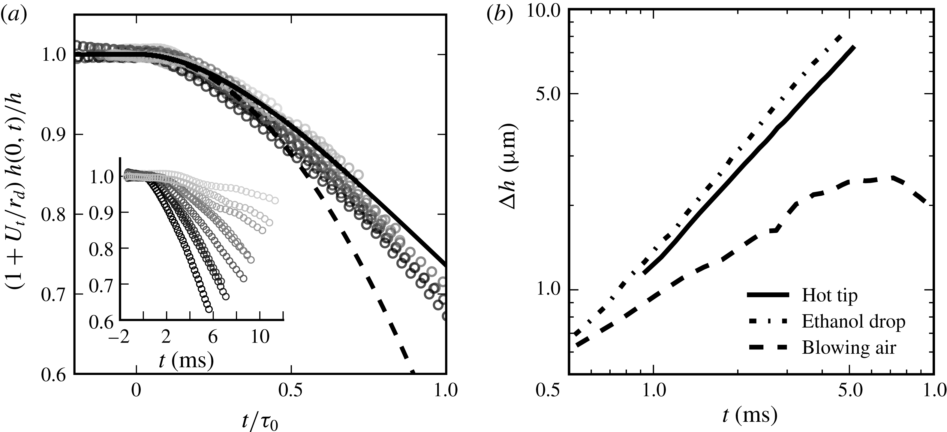
For given film velocity
 $U$
and radial location of the perturbation
 $r_{d}$
, the only tuneable parameter is
 $\unicode[STIX]{x1D70F}_{0}$
, which is varied by changing the evaporating droplet–liquid sheet distance (see § 4.4). Figure 14(a) shows the film minimal thickness
 $h(0,t)$
, rescaled by the substrate decreasing thickness
 $h/(1+Ut/r_{d})$
, as a function of time
 $t$
, for different
 $\unicode[STIX]{x1D70F}_{0}$
, measured by fitting expression (4.9) on the experimental data. The film thickness decrease is faster and deeper when
 $\unicode[STIX]{x1D70F}_{0}$
is shorter, and consistently all curves collapse on the same master curve, well represented by the expected trend, although the film seems to thin even faster than expected from (4.9).
These experiments on the Savart sheet produce a modest, though dramatically evolving, relative thickness decrease, but do not exhibit film puncture per se, because the sheet is naturally bounded. Instead of puncturing a hole, film thinning results in a reduction of the sheet radius (see (2.2)), the location where incoming radial momentum is equilibrated by surface tension retraction: since the film is thinner, it carries less momentum and therefore the equilibrium is reached sooner, i.e. at a shorter radial distance, as seen in figure 15. Note that even the structure of the sheet rim is altered with respect to the natural case (figure 15a). Contrary to the cusped nodes running along the rim of free sheets (Gordillo et al.
Reference Gordillo, Lhuissier and Villermaux2014; Villermaux & Almarcha Reference Villermaux and Almarcha2016), the rim now features a stationary cusp that does not collect any liquid (figure 15
b). The reason is, presumably, that since surface tension is minimal in
 $x=0$
, a Marangoni stress helps to evacuate the liquid in the rim along which surface tension is gradually increasing, and prevents accumulation in a node, thus smoothing its contour (figure 15
c). Away from the disturbed zone, the rim has the usual modified cardioid shape (Taylor Reference Taylor1959b
; Clanet & Villermaux Reference Clanet and Villermaux2002).
Sheet rim retraction. (a) Unperturbed sheet, flowing from left to right. The sheet ends up in a corrugated rim. Picture is 48 mm wide. (b) Sheet perturbed by an alcohol drop decreasing locally in surface tension: the rim retracts and gets smooth. (c) Close-up view of the smooth rim.

Finally, the nature of the phenomenon discussed here is best illustrated by comparing with a perturbation of the film which does not incorporate the main ingredient of the self-amplification mechanism, that is, the Marangoni stress. Figure 14(b) shows the gradual increase of the maximal film thickness difference
 $\unicode[STIX]{x0394}h$
between the film’s thinnest and thickest points as a function of time following an injection of ethanol and heat into the film, compared to an inertial perturbation made by blowing air perpendicular to the film at
 $3~\text{m}~\text{s}^{-1}$
with a 0.6 mm in diameter tube. Although both kinds of perturbations grow at short time (at a different rate, however), the inertial air jet perturbation soon saturates and decays, while the active perturbations amplify self-sustained growth in the sense explained in § 3.3.
4.4 The penetration of the dirt: varying
$\unicode[STIX]{x1D70F}_{0}$

We have not yet addressed the way the perturbative agents released by the sources (either vapours of chemicals, or heat) penetrate into the liquid. The sources (drops of pure chemical substance or the tip of a hot pan) are suspended above the sheet, which is running at velocity
 $U$
. Obviously, the substance diffusing away from the source has to cross the air boundary layer at the surface of the liquid in order to dissolve in it. If the source is close enough to the film that it is sheared by the flow in the boundary layer, the net vapour flux directed toward the film is enhanced accordingly.
The vapour pressure
 $p_{V}$
of the chemical substance is a measure of the concentration of vapour in air close to the source, and its ability to dissolve in the liquid is measured by Henry’s law constant
 $k_{H}$
. Since the liquid surface tension is lowered in proportion to the pollutant concentration dissolved in it (3.1), and since the overall transfer process from the source to the film involves linear relationships in concentration, it is clear that the surface tension deficit will be such that
 $$\begin{eqnarray}\unicode[STIX]{x0394}\unicode[STIX]{x1D70E}\sim p_{V}k_{H}\times f(\unicode[STIX]{x1D6FF}/a),\end{eqnarray}$$
where
 $f(\unicode[STIX]{x1D6FF}/a)$
is a decreasing function of the distance
 $\unicode[STIX]{x1D6FF}$
of the source to the film, and
 $a$
is the source size, provided
 $\unicode[STIX]{x1D6FF}$
is smaller than the air (viscosity
 $\unicode[STIX]{x1D708}_{a}$
) boundary layer thickness
 $\sqrt{\unicode[STIX]{x1D708}_{a}r_{d}/U}$
at the radial location
 $r_{d}$
of the perturbation above the film.
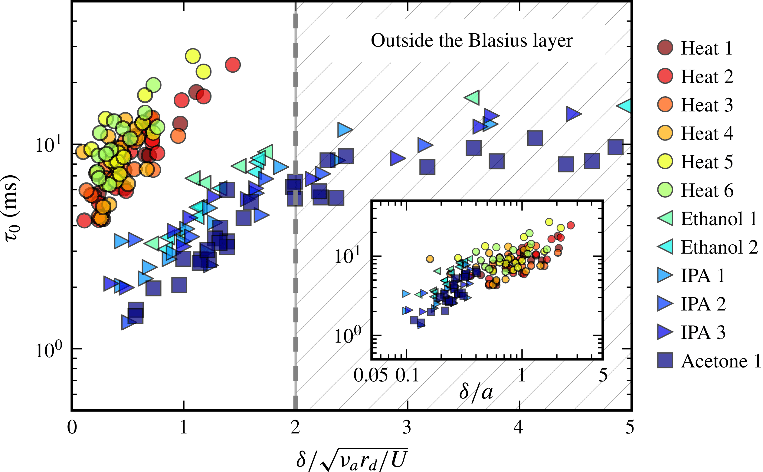
Figure 16 shows how
 $\unicode[STIX]{x1D70F}_{0}$
is large when the source stands above the air boundary layer, that it decays rapidly (indicating an increase in
 $\unicode[STIX]{x0394}\unicode[STIX]{x1D70E}$
or a decrease in the apparent dirt size
 $a$
and film thickness
 $h$
) – see (3.11) as the source approaches the film – and that
 $\unicode[STIX]{x1D6FF}/a$
is indeed the relevant scaling variable (inset). Despite their respective different
 $p_{V}$
and
 $k_{H}$
, acetone, ethanol and isopropyl alcohol (IPA) behave close to identically, precisely because their respective products
 $p_{V}k_{H}$
are very similar, as can be seen from table 1. Moreover, since molecular and heat transfer from the sources (drop or hot pan tip) to the film occurs by diffusion in the air, thus with similar diffusivities (the Lewis number in gases is of order unity), the data for heat contamination align accordingly.
The graph in figure 16 refers to the particular method we have chosen to introduce the ‘dirt’ on the film. It confirms that even weak fluctuations of composition in the air around it can trigger the spontaneous instability of the film. Of course, if any aerosol of pure substance coalesces with the film, the consequence is immediately dramatic, as illustrated in § 2.4. Similarly, any immiscible droplet or micro-bubble in the liquid, smearing the film with traces of pollutants, may trigger film rupture.
Instability time scale
 $\unicode[STIX]{x1D70F}_{0}$
measured for different solicitations, plotted versus the distance from the perturbation to the sheet
 $\unicode[STIX]{x1D6FF}$
, scaled by the thickness of the Blasius boundary layer. The diverse runs correspond to different film velocities when the perturbation is chemical, or decreasing the temperature of the tip from
 $450\,^{\circ }\text{C}$
(Heat 1) to
 $200\,^{\circ }\text{C}$
(Heat 6) by steps of
 $50\,^{\circ }\text{C}$
, with no noticeable influence. In the inset,
 $\unicode[STIX]{x1D70F}_{0}$
is plotted against
 $\unicode[STIX]{x1D6FF}/a$
, with
 $a$
the size of the perturbation, for data inside the boundary layer (
 $\unicode[STIX]{x1D6FF}/\sqrt{\unicode[STIX]{x1D708}_{a}r_{d}/U}<2$
).
5 Conclusion
Often, the reasons invoked to explain the puncture of liquid films are either the existence of attractive van de Waals forces or thermal fluctuations. These ingredients are usually considered as sufficient, while we know that they are likely to operate on films at most a few tens of nanometres thick only. However, it has also been known for at least 60 years that much thicker liquid films nucleate holes spontaneously, in a variety of different situations. It is this paradox which has prompted the present work.
The paradigm is that liquid surfaces are always somewhat dirty, to some extent, and that even a minute amount of dirt is enough to initiate puncture.
The precise meaning of ‘dirt’ refers to any agent diluted in the liquid, which is liable to lower its surface tension and therefore, through a Marangoni mechanism which we have shown to be self-sustained, to dig the film down to rupture. If a deficit of surface tension
 $\unicode[STIX]{x0394}\unicode[STIX]{x1D70E}$
is applied on a dirty spot of size
 $a$
on a liquid film of density
 $\unicode[STIX]{x1D70C}$
and thickness
 $h$
, an interstitial flow depletes the spot within a time
 $\unicode[STIX]{x1D70F}_{0}=\sqrt{\unicode[STIX]{x1D70C}ha^{2}/\unicode[STIX]{x0394}\unicode[STIX]{x1D70E}}$
, emptying and puncturing the film provided molecular diffusion of the dirt along the film has not regularised it in the meantime. Self-amplification thus occurs as soon as the Péclet number
 $Pe=a^{2}/D\unicode[STIX]{x1D70F}_{0}$
is larger than unity. For instance, a
 $100~\unicode[STIX]{x03BC}\text{m}$
spot of ethanol dissolved into a
 $10~\unicode[STIX]{x03BC}\text{m}$
thick liquid film with typical deficit of
 $\unicode[STIX]{x0394}\unicode[STIX]{x1D70E}\sim 0.1~\text{mN}~\text{m}^{-1}$
ruptures in
 $\unicode[STIX]{x1D70F}_{0}\sim 1~\text{ms}$
with
 $Pe=10^{4}$
. We have explained that one way to understand the condition
 $$\begin{eqnarray}Pe>1\end{eqnarray}$$
is to note that it is equivalent to
 $$\begin{eqnarray}\sqrt{\unicode[STIX]{x0394}\unicode[STIX]{x1D70E}/\unicode[STIX]{x1D70C}h}>D/a,\end{eqnarray}$$
stating that the film Taylor–Culick velocity constructed with the surface tension deficit
 $\unicode[STIX]{x0394}\unicode[STIX]{x1D70E}$
should be larger than the diffusion spreading velocity of the initial spot. For a film with typical thickness
 $h=10~\unicode[STIX]{x03BC}\text{m}$
contaminated with a surface tension deficit
 $\unicode[STIX]{x0394}\unicode[STIX]{x1D70E}=0.1~\text{mN}~\text{m}^{-1}$
, the cross-over size
 $a$
is approximately 10 nm, much smaller than all the perturbation sizes shown here, which consistently puncture the film provided they have the chance to penetrate it (with no rebound or evaporation if the perturbation is a drop projected over the film as in figure 8
b).
The corresponding scenario was suggested by contemplating precise experiments in different ways, either by spraying water films with droplets of soluble chemicals such as ethanol or by perturbing the vapour or temperature field at the surface of a stationary water Savart sheet. In the latter configuration, precise measurements of the instability early dynamics were obtained, including the direct proof of the existence of an interstitial flow, the shape of the resulting film thickness profile, the rate of depletion at the perturbed spot centre and the intensification of the film thickness gradients at the periphery of the spot. These were all interpreted as evidence of a self-amplified mechanism digging the film, irrespective of the nature of the perturbing agents (chemical or heat) provided they induce a surface tension deficit at sufficiently large
 $Pe$
, which was always the case in these experiments. The corresponding time scale
 $\unicode[STIX]{x1D70F}_{0}$
was measured, even if the precise nature of the singularity, if any, leading to film thickness cancellation, remains an open issue.
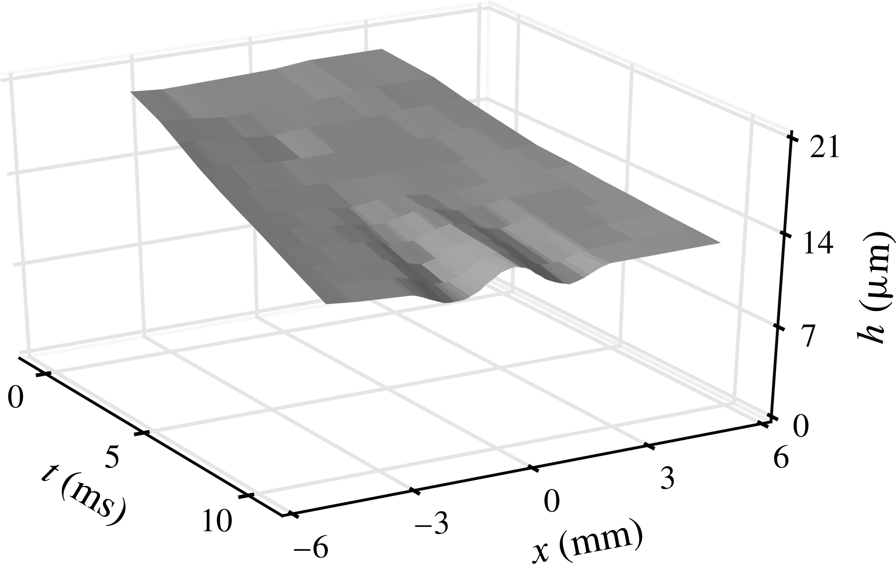
In addition, when the roles in the experiment are inverted, namely when one considers the perturbation of an ethanol sheet by the vapour coming from a water droplet, the effect subsists, but with an opposite sign, the interstitial flow now concentrating the peripheral liquid at the centre of the spot (figure 17, to be compared with figure 13).
Measured thickness field for an excess of surface tension in the dirty spot (water drop close to an ethanol sheet,
 $a=1.5~\text{mm}$
,
 $r_{d}=56~\text{mm}$
giving
 $\unicode[STIX]{x1D6FC}=1.5^{\circ }$
). The interstitial liquid is now concentrated at the centre of the spot, instead of being expelled at its periphery (see figure 13 for comparison).
Dirtiness is a feature of nature (Jacob Reference Jacob1987). The mechanism discussed here is therefore likely to be generic: minute fluctuations of composition of the atmosphere around a liquid film, any floating aerosol coalescing with it can trigger this spontaneous mechanism ending with rupture, as will any immiscible droplet or micro-bubble in the liquid, smearing the film with traces of pollutants.
Films in nature are sometimes armoured with surfactants and we have shown in figure 6 how a layer of surfactant prevents an approaching ethanol droplet from puncturing the film, a puncture which otherwise occurs before the droplet has touched a clean film. The surface or ‘spreading’ pressure (Fowler & Guggenheim Reference Fowler and Guggenheim1952) of a layer of mobile molecules with surface concentration
 $\unicode[STIX]{x1D6E4}$
is, in the diluted limit,
 $\unicode[STIX]{x1D719}=\unicode[STIX]{x1D6E4}k_{B}T$
. The work spent opening a spot of radius
 $a$
depleted in surfactant by an amount
 $\unicode[STIX]{x0394}\unicode[STIX]{x1D6E4}$
is proportional to
 $a^{2}\unicode[STIX]{x0394}\unicode[STIX]{x1D719}$
, so that in place of (3.6), we have in that case
 $$\begin{eqnarray}\displaystyle \unicode[STIX]{x2202}_{t}v=\frac{2}{\unicode[STIX]{x1D70C}h}\unicode[STIX]{x2202}_{x}(\unicode[STIX]{x1D70E}-\unicode[STIX]{x1D719}), & & \displaystyle\end{eqnarray}$$
making it clear that a surfactant coated film is shielded against the Marangoni surface contamination mechanism studied here.
The present observations are consistent with those of Vernay et al. (Reference Vernay, Ramos and Ligoure2015) who were using oil droplets loaded with surfactants partially miscible in water as perturbation agents, introduced in the bulk of the liquid. They too observed film digging and thickness gradient steepening prior to puncture. Our findings provide a mechanistic interpretation of these facts, relying on the onset of a local interstitial flow depleting the film, rather than the growth of a viscous boundary layer across the film, which would result in film thickening rather than thinning. In fact, momentum transfer across the film occurs very early in the process. It is completed within a time
 $h^{2}/\unicode[STIX]{x1D708}$
while puncture takes
 $\unicode[STIX]{x1D70F}_{0}$
. As long as
 $h^{2}/\unicode[STIX]{x1D708}\ll \unicode[STIX]{x1D70F}_{0}$
, that is for films thinner than
 $$\begin{eqnarray}h_{\star }\sim \left(\frac{\unicode[STIX]{x1D702}\unicode[STIX]{x1D708}a^{2}}{\unicode[STIX]{x0394}\unicode[STIX]{x1D70E}}\right)^{1/3},\end{eqnarray}$$
the plug flow description we have opted for holds, even if contamination time
 $h^{2}/D$
is much larger for species with
 $Sc\gg 1$
. With
 $a=100~\unicode[STIX]{x03BC}\text{m}$
and
 $\unicode[STIX]{x0394}\unicode[STIX]{x1D70E}=0.1~\text{mN}~\text{m}^{-1}$
on a water film, we have
 $h_{\star }\approx 50~\unicode[STIX]{x03BC}\text{m}$
, and we have seen in figure 10 that even films as thick as
 $250~\unicode[STIX]{x03BC}\text{m}$
are sensitive to the effect we have described.
Finally, we would like to mention the profound analogy existing between the mechanism for hole nucleation in a locally dirty liquid film, and the phenomenon of flame ignition in the combustion of premixed reactants undergoing an exothermic reaction (Frank-Kamenetskii Reference Frank-Kamenetskii1969; Zeldovich et al.
Reference Zeldovich, Barenblatt, Librovich and Makhviladze1985). Combustion refers to this class of reactions which are exothermic, and whose reaction kinetics is strongly activated by temperature. Let
 $k$
be the (temperature dependent) reaction rate, and
 $a$
the size of a spot in the mixture where some thermal energy has been released, thus elevating locally the temperature. Ignition of the mixture will occur provided the temperature in the spot remains high enough during a time of the order of
 $k^{-1}$
at least for the reaction, which is exothermic thus sustaining flame propagation, to proceed. If
 $D$
is the heat diffusivity, the condition above reads
 $ka^{2}/D\gg 1$
, which is the precise equivalent of our large Péclet number (3.12)–(5.1) condition for hole nucleation.
Acknowledgement
The Agence Nationale de la Recherche (ANR) is acknowledged for funding of the grant ANR ‘FISICS’ ANR-15-CE30-0015-03.
Appendix A. Dynamics of a front
Broad support of surface tension deficit. (a) Measured thickness field for an ethanol source of size
 $L=4.6~\text{mm}$
. The thickness decreases at the edges of the source. (b) Sheet rim double retraction, with an even larger perturbation
 $L=10~\text{mm}$
. Two cusps appear, signatures of the two decoupled thickness decreases.

We have up to now considered a spot of dirt with a single length scale, namely its radius
 $a$
. It may happen that the dirt is deposited on the film over a broader support, say of size
 $L\gg a$
, with smooth cross-overs of the pollutant concentration at the periphery of the spot over a width, say,
 $a$
. In that case, illustrated in figure 18, a dynamics very similar to the one described in § 3 distorts an initially flat film. We consider an initially smooth cross-over of the surface tension as
 $$\begin{eqnarray}\displaystyle & \displaystyle \unicode[STIX]{x1D70E}(x,t=0)=\unicode[STIX]{x1D70E}+\frac{\unicode[STIX]{x0394}\unicode[STIX]{x1D70E}}{2}\text{erf}\left(\frac{x}{a}\right), & \displaystyle\end{eqnarray}$$
 $$\begin{eqnarray}\displaystyle & \displaystyle \text{so that }\unicode[STIX]{x2202}_{x}\unicode[STIX]{x1D70E}|_{t=0}\sim \frac{\unicode[STIX]{x0394}\unicode[STIX]{x1D70E}}{a}\text{e}^{-(x^{2}/a^{2})}. & \displaystyle\end{eqnarray}$$
From (3.7), the interstitial fluid velocity is
 $$\begin{eqnarray}v(x,t)\sim \frac{ta}{\unicode[STIX]{x1D70F}_{0}^{2}}\text{e}^{-(x^{2}/a^{2})},\end{eqnarray}$$
where
 $\unicode[STIX]{x1D70F}_{0}$
is given by (3.11). The symmetry being broken in the initial condition, when compared to a bell-shaped initial
 $\unicode[STIX]{x1D70E}$
-deficit the velocity is positive everywhere (see figure 19
a). Solved in the slender slope limit
 $\unicode[STIX]{x2202}_{x}h\ll 1$
, mass conservation in (3.4) provides the thickness field
 $h(x,t)$
as
 $$\begin{eqnarray}\frac{h(x,t)}{h}=\exp \left\{\left(\frac{t}{\unicode[STIX]{x1D70F}_{0}}\right)^{2}\frac{x}{a}\text{e}^{-(x^{2}/a^{2})}\right\},\end{eqnarray}$$
with
 $h$
the initial film thickness. Liquid is flowing towards positive
 $x$
, collecting into a bump located in
 $x=a/\sqrt{2}$
, and digging in
 $x=-a\sqrt{2}$
(figure 19
b).
Time evolution of an initial step of surface tension of width
 $a$
, for different Péclet numbers. Graphs are centred around
 $x=a/\sqrt{2}$
, where compression is maximal. (a) Interstitial velocity and (b) film thickness for
 $Pe=+\infty$
(or equivalently short times
 $t/\unicode[STIX]{x1D70F}_{0}\ll 1$
). (c–d) Surface tension profiles at successive times, for two finite Péclet numbers.
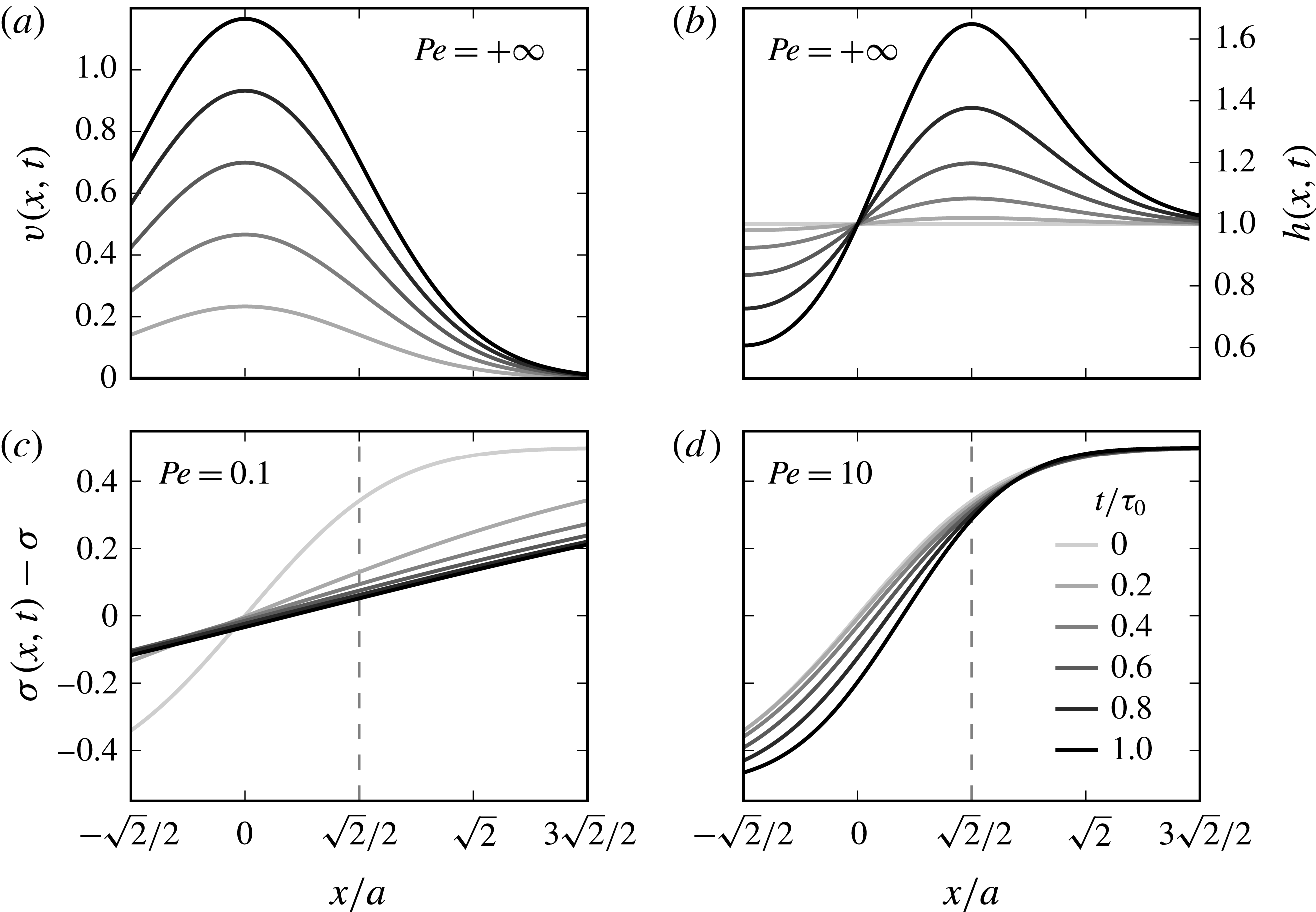
The maximal rate of compression
 $\unicode[STIX]{x1D6FE}$
along the film is now obtained in
 $x=a/\sqrt{2}$
, and increases linearly with time
 $t$
as in (3.13). The negatively sloped velocity expands about that point as
 $v(x,t)=v(a/\sqrt{2},t)-\unicode[STIX]{x1D6FE}\tilde{x}$
, with
 $\tilde{x}=x-a/\sqrt{2}$
. The mixing analogy maps the problem onto a pure diffusion equation, as in § 3, with the same conclusions. The diffusion equation (3.18) is solved in this particular case to give an explicit expression for
 $\unicode[STIX]{x1D70E}(x,t)$
,
 $$\begin{eqnarray}\displaystyle & \displaystyle \unicode[STIX]{x1D70E}(x,t)=\unicode[STIX]{x1D70E}+\frac{\unicode[STIX]{x0394}\unicode[STIX]{x1D70E}}{2}\text{erf}\left(\frac{\unicode[STIX]{x1D709}(x,t)+{\displaystyle \frac{\sqrt{2}}{2}}}{\sqrt{1+4\unicode[STIX]{x1D70F}(t)}}\right), & \displaystyle\end{eqnarray}$$
with
 $$\begin{eqnarray}\unicode[STIX]{x1D709}(x,t)=\frac{x-{\displaystyle \frac{\sqrt{2}}{2}}}{s(t)},\quad \unicode[STIX]{x1D70F}(t)=D\int _{0}^{t}\frac{\text{d}t^{\prime }}{s(t^{\prime })^{2}}\quad \text{and}\quad s(t)=a\text{e}^{-(t^{2}/2\unicode[STIX]{x1D70F}_{0}^{2})}.\end{eqnarray}$$
Figure 19(c,d) illustrates how the
 $\unicode[STIX]{x1D70E}$
-fields relaxes for
 $Pe<1$
, and steepens for
 $Pe>1$
in the self-sustained amplification regime.



