2. SPACE TEST BED AND SOFTWARE SUITE

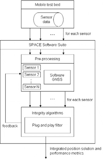
The plug and play integration filter forms one part of the software known as the SPACE Software Suite (SSS). The SSS forms the software part of the SPACE test bed and is used to combine the measurements from the different sensors to provide a position solution. The high level architecture of the SPACE test bed and SSS is shown in Figure 1. The figure shows that the main function of the mobile test bed is to collect data from all available sensors and log the data to a file. The main sensors to be initially considered for integration on the test bed are:

• — GNSS (including modernized GPS and Galileo)

• — INS

• — Pseudolites

• — Dead reckoning

• — Ultra wideband

• — Bluetooth ranging

• — Imaging sensors.

However, this is not a restrictive list and the aim of the integration filter is to provide an interface for most positioning technologies. An important part of the data collection is the time synchronisation of the data (this is considered in detail later in this paper) and all data is stored with a GPS time stamp (obtained using a GPS receiver operating in real-time) on a hard disk which is later used with the SSS in post processing. The initial implementation of the software part of the test bed will be in post processing. However it is planned that the future test bed will be able to operate in real-time, therefore only algorithms that can potentially operate in real-time are used in the software.

Figure 1.

High level flow diagram for SSS.

The figure shows that once the data has been collected, it is used in the SSS. The first part of the SSS is the pre-processing step where the recorded measurements from the test bed are processed as necessary to provide inputs for the plug and play filter. A significant part of this is the software GNSS receiver. The test bed will contain a RF front end and data logger that will capture high bandwidth RF signals. This will be used instead of using a GPS receiver that would only record the raw pseudorange and carrier data. This provides the capability to replay RF scenarios which can be processed with different receiver algorithms in post processing. The output of the software GNSS will be code, carrier and Doppler measurements as well as some additional parameters such as signal to noise ratio and loss of lock indicators. The measurement data from the other sensors carried on the test bed, such as Inertial Measurement Units (IMUs) and UWB will be recorded, although only GNSS signals will be captured at the RF level. The pre-processing step is required for tasks such as numerical integration of the raw IMU data, computation of satellite positions from ephemeris data and cycle slip detection.

The pre-processing algorithms are used to get the data in a format ready to be used with the plug and play filter as described in the following sections. The plug and play filter will be controlled by the integrity part of the SSS. The integrity algorithms will be used to monitor the states of the Kalman filter and remove or flag bad data (the integrity algorithms are not described in this paper). In the final step, the navigation solution is computed by the filter and output to a file. The filter output can also be used as a feedback signal to control errors such as INS drift, and to provide an aiding signal, for example, to aid signal tracking and acquisition in the software GNSS receiver (commonly referred to as deep integration).

3. PLUG AND PLAY FILTER

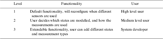
The first issue to be addressed in the development of the plug and play filter was the definition of ‘plug and play’. The intention was to make the filter as adaptable as possible, but it is impossible to identify all future sensor combinations or measurement types. Therefore three different levels of functionality were identified which require different levels of user knowledge and interaction. These levels are summarised in Table 1. The highest level user is level 1, where the software is used to provide default functionality with default algorithms implemented for different sensors. In this case, all that is required from the user is the selection of navigation sensors to carry on the test bed. This will make the filter easy to use and will require no knowledge of the algorithms used.

Table 1.

User levels for plug and play filter.

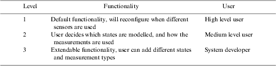
The second level allows the user to decide which states are modelled (for example different INS error models), and how the measurements are used (for example different differencing strategies for GNSS observations). In this case, the software can be configured by means of a user interface without having to reprogram source code. This level will be used to find the optimum processing strategy for integrating the different sensors. The final user level is a low level user functionality where the source code can be modified to provide extended functionality such as adding different states or new measurement types. An Interface Control Document (ICD) will be provided with a strict definition of how the states and measurements should be implemented in the source code. This effectively future proofs the filter for any sensor combinations that are not considered in the current form of the plug and play filter. The following sections describe the low level development of the filter.

4. INTEGRATION ALGORITHM

There are a number of algorithms suitable for integrating navigation sensors. Of these the most commonly used is the Extended Kalman Filter (EKF), but recently other algorithms such as Unscented Kalman filters (e.g. Shin, Reference Shin2005), Particle filters (e.g. Bergman Reference Bergman1999) and neural networks (e.g. Noureldin et al Reference Noureldin, Sharaf, Osman and El-Sheimy2004) have been investigated. Alternative algorithms to the EKF have mainly been used to address the problem of linearization which is required in order to model non-linear systems in the Kalman filter. However, for the application of centimetre level positioning, the effect of higher-order non-linearities are unlikely to have a significant impact on the positioning performance. Other advantages such as reducing the requirement for deriving Jacobian matrices for the system and observation equations do have some benefit for the plug and play filter. However, the EKF was chosen primarily because of its efficiency, especially for applications where there are a large number of states and observations.

Once the EKF algorithm had been chosen, it was necessary to identify the different parts of the Kalman filter that could be configured automatically, and where values must be provided by a user. The Kalman filter equations for the extended Kalman filter are defined as:

(1)

(2)

(3)

(4)

(5)

(6)

where:

x

is the state vector

P

is the covariance matrix

Φ

is the state transition matrix

Q

is the process noise

z

is the measurement vector

H

is the design matrix

R

is the measurement noise matrix

K

is the Kalman gain

and (−) and (+) denote predicted and updated values respectively, the subscript k denotes the current epoch k, and the notation k−1|k describes the interval from epoch k−1 to k. Equations 1 and 2 are known as prediction, and 3 to 6 are the update equations.

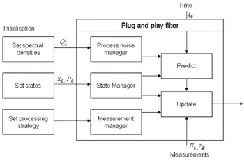
To begin the Kalman filter, the user must define which states are to be modelled (x) and their initial estimates (x ₀), an estimate of the initial uncertainty (P ₀), and the process noise (Q). The user must also define which measurements are to be used (z) and their statistical properties (R). For some sensors it is also necessary to define how the measurements are used (such as linear combinations or double differencing). Most importantly from these equations, it is identified that the state transition matrix, and the design matrix can be automatically populated by the software depending on the defined states and measurements. The process noise matrix can also be formulated as described in the following sections based on the definition of the spectral density matrix which defines where the noise enters the system.

Figure 2 shows the configuration of the plug and play filter. The plug and play filter is coded using the c++ programming language, and three classes are defined which form the process noise, state and measurement managers. The process noise and state managers are very simple classes that define which system noise inputs and states are to be modelled. The measurement manager is used to store measurements, and also provides differencing algorithms as described later in this paper. These three classes are configured by a set of configuration commands that are controlled by the user interface (this provides the functionality for user level 2). These classes are then used to populate all the required matrices (Equations 1 to 6) for the Kalman filter prediction and update equations as described in the following sections.

Figure 2.

Plug and play filter flow diagram.

5. STATES AND PROCESS NOISE

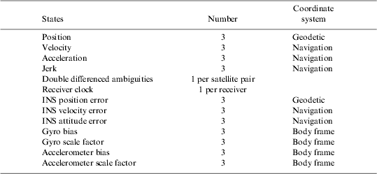
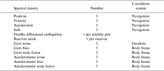
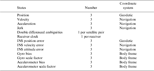
Table 2 shows the states that are currently modelled within the SSS. Any combination of these states can be used, including, for example, subsets of position such as latitude and longitude only. Future developments are expected to update the Kalman filter to include double differenced L1 ionospheric error, zenith tropospheric delay states, additional IMU errors such as temperature dependent bias states and misalignment states, a large angle error model for the INS attitude error states (see, for example, Shin Reference Shin2005), dead reckoning error models, and estimation of lever arm separation between sensors. These states can be added to the respective manager classes, as long as the developer can define the partial derivates and dynamics equations to form the design and state transition matrices as described in the following sections.

Table 2.

States modelled in plug and play filter.

6. PROCESS NOISE MATRIX

The process noise matrix describes the uncertainty of the states as they are predicted over time. This is formed using the definition of the spectral density matrix Q _s handled by the process noise manager. The process noise matrix is defined as:

(7)

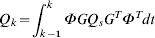
where G is the matrix that relates the input noise to the states over the interval dt=t _k−t _k−1. The matrix G can be automatically generated using the states and spectral density matrix based on known equations. The plug and play filter uses the following numerical approximation to compute the process noise matrix (Maybeck, Reference Maybeck1994):

(8)

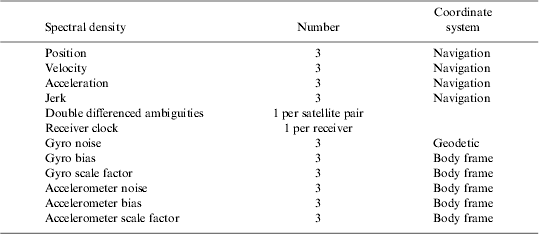
Table 3 shows the current spectral density inputs that are modelled in the plug and play filter. Again, this can be easily extended, with the developer needing to define the relationship matrix G between each input and the states.

Table 3.

Process noise modelled in plug and play filter.

7. STATE TRANSITION MATRIX

The dynamics matrix, F, describes the relationship of the states over time. When the dynamics matrix can be considered to be constant over a short interval, the state transition matrix is formed using the equation:

(9)

This numerical expansion is used in the plug and play filter. The dynamics matrix is formed using the INS error models as described in, for example, Farrell and Barth (Reference Farrell and Barth1999). In the absence of an INS, a dynamic model can be used; these are of the form of constant position, velocity, acceleration or jerk (rate of acceleration) models. By only specifying the dynamics matrix, it is necessary to expand Equation 9 to a significant number of terms to fully describe the dynamics of the system.

8. MEASUREMENTS

The measurements for the plug and play filter are categorised into different measurement types. These comprise position, velocity, attitude, range and range rate (Doppler) observations. The source code interface to the plug and play filter is very important since information is required for all the properties of each measurement so that the plug and play filter can automatically populate the design matrix, and compute the predicted value for the extended Kalman filter. Measurements are added to the measurement manager using the following definitions.

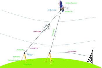
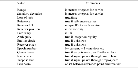
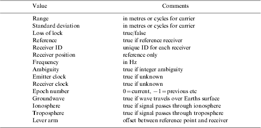
Range measurements are the principal measurements that are used in the plug and play filter, since this is how the majority of positioning sensors operate. Figure 3 shows a diagram of the different attributes of range measurements for different sensors. The attributes are summarized in Table 4. The attribute table effectively provides a ‘form’ that is filled out for each measurement which is added to the Measurement Manager. The table describes all properties of range measurements which are principally used to form the design matrix, defined as:

(10)

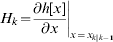
where ∂h[x] is the non-linear function of the states. The elements of this matrix must be defined by the system developer. The plug and play filter can then populate the matrix depending on the states and measurements used. Similar attribute tables are formed for the position, velocity and attitude measurements, with the position table shown in Table 5.

Figure 3.

Attributes of range measurements.

Table 4.

Attribute table for range measurements.

Table 5.

Attribute table for position measurements.

The attributes are required when using, for example, GNSS positioning. For example, it is necessary to know properties about the signal path if states are modelled for ionosphere and troposphere, so the relevant partials for these states can be formed. Some properties are also required in order to compute the predicted range measurement for the Extended Kalman filter. In particular, it is necessary to know the emitter position, receiver position and whether the signal has passed directly through the atmosphere, or has travelled across the surface of the Earth. For range rate measurements, the attribute table is very similar to the range table, except for the addition of emitter and receiver velocities which are necessary to be able to form the predicted range rates and partial derivates.

9. DIFFERENCING

For applications such as GNSS positioning, ranges are typically differenced with reference receiver ranges to form either single, double or even higher order differences to remove or mitigate the common errors between observations. Unfortunately, this complicates the design of the Kalman filter when differenced observations have to be considered. One option is to extend the number of observation types to include single differenced ranges, and double differenced ranges. Alternatively, all ranges can be passed to the plug and play filter and then perform the differencing scheme inside the Kalman filter. The latter approach was chosen principally so that correlations between observations could be correctly modelled, but also because additional ‘house-keeping’ tasks are required when using differenced measurements such as when the base satellite for differenced observations changes. Therefore, in the plug and play filter, an additional differencing step was added.

Differencing observations are achieved in the plug and play filter by use of the differencing matrix, D. The differencing matrix is formed using the user configuration information stored in the Measurement Manager. First the standard un-differenced Kalman filter measurement equations are formed. For example, for four ranges ρ₁ to ρ₄, the observed minus predicted residual vector is formed as:

(11)

where δρ₁ is the difference between the observed and predicted range ρ₁. Assuming that the ranges can be considered uncorrelated, the measurement noise matrix for the un-differenced measurements is formed using the matrix:

(12)

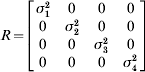
where σ₁ is the standard deviation of the range error. The design matrix is formed from the Jacobian matrix in Equation 10 for each state. To form the single difference for the ranges, with the 4th range defined as the reference satellite, the following differencing matrix is used:

(13)

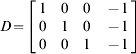
The differencing matrix can then be applied to give the equivalent matrices for the single differenced scheme by using the equations:

(14)

(15)

(16)

where ()_∇ denotes the signal difference. By using this approach to form the observations for the plug and play filter, the mathematical correlations between measurements are preserved, which is particularly important with the formulation of the measurement noise matrix. The code required to implement the difference scheme is very simple and scaleable. For example, it can also be used to form linear combinations of measurements, such as the ultra-widelane and widelane combinations of GNSS observations (although care must be taken to correctly scale the measurements in terms of frequencies to ensure the correct modified wavelength is computed). One problem with this approach is that the differencing matrix becomes very large when considering a large number of observations. To address this problem, pointers are used in the software implementation to handle the sparse matrix that is generated which results in a relatively efficient implementation of the algorithm.

10. AMBIGUITY RESOLUTION

Integer ambiguity resolution is one of the necessary steps to achieve centimetre level positioning using carrier phase GNSS observations. Although it is not specifically a Kalman filtering task, it was decided that ambiguity resolution would be included within the plug and play filter, as opposed to considering it as a separate task. This is because tasks such as rearranging the double differenced ambiguity states when the reference satellite changes, removing ambiguity states when they are fixed and updating states with the fixed values are all necessary, and would require additional interfaces to the plug and play filter.

An additional integer ambiguity search was added to the plug and play filter to resolve double differenced ambiguities. The LAMBDA algorithm (De Jonge and Tiberius, Reference De Jonge and Tiberius1996) is used to decorrelate the ambiguities to make the integer ambiguity search more efficient. Ambiguity validation is currently achieved using the ratio test (Teunissen, Reference Teunissen2005) but this is likely to be modified in future versions. Once the ambiguities have been resolved, it is necessary to remove the ambiguity states from the state vector of the Kalman filter, as well as to update the remaining states with the resolved integer values. This is achieved by using the following ambiguity decorrelation equations:

(17)

(18)

(19)

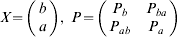
where X is the original state vector partitioned into a which are the ambiguity states to be removed, and b which are the remaining states. The matrix P is the corresponding covariance matrix. Equations 18 and 19 are then used where â denotes the vector of correctly resolved integers and and P are the new state vector and covariance matrix respectively. Implementing ambiguity estimation in this way allows for the Triple Carrier Ambiguity Resolution (TCAR) algorithm to be used (see, for example, Teunissen et al, Reference Teunissen, Joosten and Tiberius2002), which resolves ambiguities in a cascading fashion, starting with long wavelength measurements which have ambiguities that are easy to resolve, moving down to shorter wavelength signals. In fact, using a combination of the differencing algorithm and the ambiguity resolution algorithm described means that any number of different linear combinations of observations can be estimated and resolved in the plug and play filter.

11. TIME SYNCHRONIZATION

Time synchronization is an important consideration for multi-sensor systems. It is essential that all sensors are time synchronized, since for kinematic applications, time errors directly propagate into position errors between sensors. The requirements for time synchronization are dependent on the required accuracy of the application and the velocity of the vehicle. For centimetre level positioning, synchronization requirements are very stringent even at low speeds. For example, a typical walking speed is 5 km/h which equates to approximately 1·4 m/s which means that a synchronization error of 0·01 s will result in 1·4 cm error.

For the SSS, the requirement for the test bed is that all sensors are synchronized relative to GPS time. Since the software works in post processing, data must be written to a file with a GPS time stamp. Currently, a standard interface for different positioning sensors does not exist, therefore each sensor on the test bed will generally need to have a custom synchronization interface developed. Most current IMUs have serial data interfaces, and the only way to synchronise their output is to time stamp the serial data as its output from the device. Generally, this is achieved using custom data loggers developed by system integrators for each type of IMU. For the SPACE test bed, a generic data logger has been developed that can time stamp the data from any serial device with an accurate time stamp to an estimated accuracy of better than 0·1 ms. The data logger can also be used with any serial sensor where the delay between the measurement being sampled and output is constant. Other devices will require a custom interface to be developed. The most common way to achieve this is to output a synchronization pulse as the measurement is sampled from each sensor. The synchronization can be time tagged using the SPACE data logger, and in post processing, the logged time is matched with the logged data.

One potential problem that arises with multi-sensor systems is that the measurements from asynchronous sensors are not necessarily sampled at the same time. In situations where partial measurements from different systems are available (for example two GPS satellites and two UWB ranges), it is advantageous for the measurements to be acquired simultaneously so that an accurate position can be obtained from the combination of measurements. It is recognised that it is unlikely to be achievable when using sensors from different manufacturers. Therefore the SPACE test bed alleviates the need for obtaining simultaneous measurements by using an INS. Using a tactical grade or better IMU, the observations can be used at the time the measurement is taken to update the INS. The INS is therefore able to make use of all of the aiding measurements as they are available. The alternative is to use a dynamic model in the Kalman filter, however this is unlikely to be suitable unless the dynamics of the platform can be well modelled considering that centimetre level positioning is the objective.

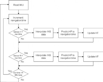
When the measurements have been time tagged and stored, the next issue to address is how the measurements are handled within the software. Figure 4 shows the flow diagram for the sensor synchronization within the SSS. Firstly, the IMU data is read and the position, velocity and attitude of the INS is updated. The software then enters a loop where the navigation time is incremented at the required resolution (typically 0·1 ms is used). The navigation time is incremented from the previous IMU time. When the time matches with one of the aiding sensors (at the resolution of navigation time), the navigation solution from the INS is interpolated to give a solution at the current navigation time. The Kalman filter is predicted (if necessary) to the current navigation time using the interpolated INS solution. The observations are formed and the Kalman filter update for that sensor is computed. One point to note is that different sensors with measurements sampled at the same time are updated using separate Kalman filter updates (instead of one single Kalman filter update step). As long as the measurements are not correlated, this approach is equivalent to using all the measurements in a single update step, plus it results in a more efficient implementation. A proof of this is given in Petovello (Reference Petovello2003). The principle drawback, however, is that techniques such as innovation residual testing become less robust due to the reduced number of observations used at one time.

Figure 4.

Sensor synchronisation flow diagram.

12. FILTER TESTING

Initial results using the plug and play filter have focussed on the integration of GPS and INS data. However, to demonstrate the full advantages of the filter, some additional measurements similar to those expected to be produced from additional ranging systems have been investigated. Some initial results with the plug and play filter have been obtained using a combination of real GPS and INS data collected in a clear open area, combined with simulated ranges from a system such as UWB. The GPS and INS data was collected on a vehicle at Aberporth airfield, Wales in August 2005 using the University of Nottingham's Applanix POS-RS. The POS-RS consists of a navigation grade Honeywell CIMU and Novatel OEM4 receiver. The vehicle was driven at various speeds and dynamics up and down the runway for a period of 40 minutes. At the beginning of the dataset, there is a 20 minute static period for alignment of the INS.

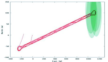
Figure 5 shows the trajectory of the vehicle along the runway. At one end of the runway, four transceivers have been simulated, and the coverage is shown in the figure. The measurements have been designed to mimic a prototype UWB system from Thales Research and Technology (Ingram et al, Reference Ingram, Harmer and Quinlan2004), although artificial coverage has been introduced for the simulation. Usually five UWB transceivers and a mobile are used with one of the transceivers acting as a master to synchronise the system. A mobile transceiver is used to record pseudoranges to the four non-masters.

Figure 5.

Vehicle trajectory along Aberporth runway, green area shows pseudolite coverage.

Synchronisation with GPS time is achieved by recording an output pulse from the mobile every UWB frame which is approximately every 11 ms. During the first half of the frame, the mobile synchronises with the master, and during the second half of the frame, the measurements to the other pseudolites are taken. The receiver selects the best of the measurements to record, which means that the recorded data is not at a constant interval. Furthermore, no two pseudoranges are recorded at the same time. The result is that the UWB system outputs ranges at a rate of approximately 5Hz with individual range measurements offset by approximately 5 ms, therefore measurements with these characteristics are simulated.

The simulation of the UWB measurements differs slightly to the prototype system which outputs a linear combination of ranges to the slave and master transmitters. Instead, the master transmitter was excluded from the simulation, and the measurement noise of each range was increased (this is to be equivalent to using differenced measurements to remove clock errors). The measurement random noise was defined to be 5 cm, and effects such as multipath were not considered. The primary purpose of the simulation was to test the ability of the filter using ranging measurements from different systems, not necessarily UWB, which may occur at different time intervals.

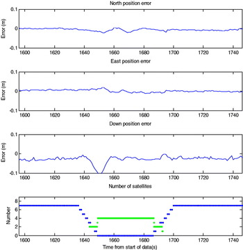
Figure 6 shows the position error (computed from the difference between the post-processed smoothed solution) for the trajectory when GPS satellites are gradually removed from the solution. The figure shows that as the satellites are removed, two UWB pseudorange observations come into view, followed by four UWB observations which corresponds to the UWB coverage shown in Figure 5. The figure demonstrates that centimetre level positioning can be retained as the integration filter combines the observations from the two different systems. During the period 1640 to 1650 seconds, it can be observed that the down position error increases as the satellites go out of view due to drift in the INS. This is not improved until the system is in the centre of the UWB coverage where the geometry is sufficient to resolve the height (the pseudolites were assumed to be fixed 10 m above the runway). It should also be noted that ambiguities are fixed in a single epoch as soon as five satellites return to view.

Figure 6.

Integrated system error using GPS, INS and simulated pseudolites during UWB trial.

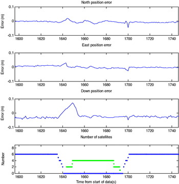
A similar plot is shown in Figure 7 except in this instance the GPS observations are removed so that there is a gap of a few seconds between GPS being removed, and pseudolites coming into view. The results show that the INS is able to maintain centimetre level position accuracy during the gap. Again, there is a drift in the vertical channel where there are less than 4 measurements in view.

Figure 7.

Integrated system error using GPS, INS and simulated pseudolites during UWB trial.

The initial results from the integration of GPS, INS and simulated pseudolites demonstrate that the software is able to seamlessly integrate different types of measurements. The simulation software also provides a useful tool for investigating the performance of different numbers and positions of pseudolites to maintain centimetre position accuracy during periods of degraded GPS. It is, however, recognized that with real data, as the test bed travels through difficult environments, the observations will not only be obstructed, but may be degraded due to effects such as multipath. Therefore, additional work will be carried out with the integrity part of the SSS to ensure quality is maintained and bad observations removed.

13. FUTURE TEST BED

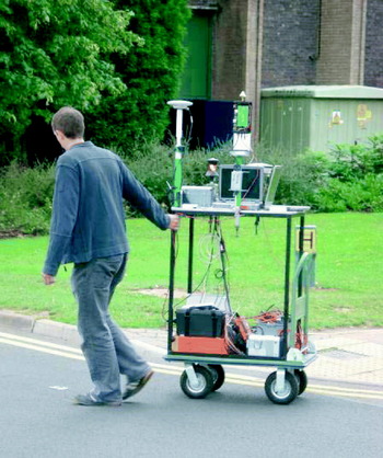
A prototype version of the test bed has been developed for operating in difficult environments. The test bed consists of the navigation grade Honeywell CIMU, a tactical grade Honeywell HG1700, a dual frequency Leica System 500 GPS receiver and a prototype UWB system from Thales, along with necessary power supplies and data logging equipment. A field trial has been conducted in Nottingham in August 2006 with 5 UWB pseudolites set up inside the main hall at the University of Nottingham sports centre. The mobile test bed, shown in Figure 8, was moved around an area that included clear open sky, close to the building and inside the building. Future work aims to demonstrate that data collected from the mobile test bed will be able to seamlessly position at the centimetre level both outdoors and inside the building.

Figure 8.

Prototype version of future test bed.