



1. Introduction
The origin of research on the interaction of oscillating bodies with a fluid dates back to the 19th century, when the first fundamental results in this area were obtained. However, large-scale diversified research in this problem area began only in the 20th century, when with the emergence of new technologies and the increasing complexity of engineering structures, the problem of oscillatory motion in a fluid acquired particular practical significance. Currently, research is conducted both in classical directions, such as wave action on offshore structures and damping of liquid oscillations in fuel tanks, and in a wide range of new applied fields: alternative energy (including wave power plants), development of high-efficiency cooling systems for microelectronics, design of oscillatory biomimetic propulsors for unmanned vehicles, development of acoustic systems for manipulation of microdevices and nanoparticles (including lab-on-a-chip and bioprinters), atomic force microscopy, development of methods for determining properties of materials and liquids, and so on (see Martin & Farina Reference Martin and Farina1997; Scherer, Frank & Gummer Reference Scherer, Frank and Gummer2000; Aureli et al. Reference Aureli, Prince, Porfiri and Peterson2010; Childress, Spagnolie & Tokieda Reference Childress, Spagnolie and Tokieda2011; Erturk & Inman Reference Erturk and Inman2011; Kopman & Porfiri Reference Kopman and Porfiri2013; Yeh & Alexeev Reference Yeh and Alexeev2014; Nama et al. Reference Nama, Huang, Huang and Costanzo2016; Shintake et al. Reference Shintake, Cacucciolo, Shea and Floreano2018; Yu, Tom & Jenne Reference Yu, Tom and Jenne2018; Ebrahimi et al. Reference Ebrahimi, Eldredge and Ju2019; Oh et al. Reference Oh, Seo, Kim and Choi2019; Yeh, Demirer & Alexeev Reference Yeh, Demirer and Alexeev2019; Lei, Cheng & Li Reference Lei, Cheng and Li2020).
Despite the long and rich history of research, the theory of periodic motion of bodies in a fluid is currently well developed only for some particular geometries. Numerous results for bodies of various shapes exist, but a systematic theory applicable to an arbitrary cross-section is absent even for two-dimensional problems at small amplitudes. The aim of the present work is to fill this gap: based on the asymptotic method, to construct a generalisation that will allow calculating the hydrodynamic forces acting on a translationally oscillating cylindrical body of arbitrary cross-section.
The flow and the corresponding hydrodynamic action on a body undergoing translational oscillations are determined by two dimensionless parameters. The first characterises the ratio of the Stokes boundary layer thickness to the characteristic body size (Landau & Lifshic Reference Landau and Lifshic1987):
 \begin{align} \varepsilon = \frac {d_{st}}{R}, \quad d_{st} = \sqrt {\frac {\nu }{\omega }}, \end{align}
where
 $\nu$
is the kinematic viscosity of the fluid,
 $\omega$
is the angular frequency of oscillations, and
 $R$
is the characteristic body size (e.g. the radius for a circular cylinder). Instead of
 $\varepsilon$
, the parameter
 $\beta = 2/(\pi \varepsilon ^2)$
, called the Stokes number or dimensionless frequency, is often used. The second parameter is the Keulegan–Carpenter number (Keulegan & Carpenter Reference Keulegan and Carpenter1958)
 \begin{align} \textit{KC} = \pi \frac {A}{R}, \end{align}
which determines the dimensionless oscillation amplitude. Here,
 $A$
is the dimensional oscillation amplitude. Asymptotic models are constructed in the region of small amplitudes (
 $\textit{KC} \ll 1$
), where separation of the unsteady boundary layer is absent. Additional conditions on the parameter
 $\varepsilon$
may be imposed depending on the physical regime to be investigated.
The following scalings are widely used:
 $\textit{KC} \ll 1$
,
 $\varepsilon$
arbitrary;
 $\varepsilon \ll 1$
,
 $\textit{KC} \sim \varepsilon ^2$
;
 $\varepsilon \ll 1$
,
 $\textit{KC} \sim \varepsilon$
, within which an asymptotic expansion can be constructed. A summary of key asymptotic studies corresponding to these scalings is presented in table 1.
Key asymptotic studies for cylinders of various shapes.

One of the first analytical studies of body oscillations in a quiescent fluid was conducted by Stokes (Reference Stokes1851). Stokes constructed a solution for the problem of a circular cylinder oscillating under the assumption of small oscillation amplitude
 $\textit{KC} \ll 1$
(for arbitrary
 $\varepsilon$
), within which the contribution of convective terms can be neglected in the first approximation. From the obtained solution, Stokes determined the hydrodynamic force
 $f_\alpha$
acting on the cylinder along the oscillation axis:
 \begin{align} f_\alpha = f^{(0)}_\alpha + O\big(\textit{KC}^2\big) = -2 \pi \operatorname {Im}\left [{\textrm e}^{{\textrm i}t}\left (1+S_x\right )\right ] + O\big(\textit{KC}^2\big). \end{align}
Here, the force is normalised by
 $\rho R^2U\omega$
, and
 $S_x = S_x(\chi )$
with
 $\chi = \sqrt {{\textrm i}/\varepsilon ^2}$
is expressed in terms of modified Bessel functions:
 $S_x(\chi ) = 2K_1(\chi )/(\chi\, K_0(\chi ))$
.
To assess the significance of convective terms, Schlichting (Reference Schlichting1932) constructed an asymptotic solution for the case
 $\textit{KC} \sim \varepsilon ^2 \ll 1$
. The terms of order
 $O(\textit{KC}^0)$
give a purely periodic Stokes solution (they coincide with (1.3) if
 $S$
is expanded in series as
 $\varepsilon \to 0$
), while the terms of order
 $O(\textit{KC}^1)$
account for the contribution of convective terms. Schlichting was the first to show that the nonlinear nature of this term leads to the appearance of a steady component in the solution – a secondary steady streaming flow arising against the background of the primary unsteady motion. A generalisation to the case of arbitrary
 $\varepsilon$
for the circular cylinder at
 $O(\textit{KC}^1)$
was obtained by Holtsmark et al. (Reference Holtsmark, Johnsen, Sikkeland and Skavlem1954).
Subsequent asymptotic studies of the circular cylinder oscillation problem under various approximations were also carried out by Andres & Ingard (Reference Andres and Ingard1953), Stuart (Reference Stuart1966), Wang (Reference Wang1968), Riley (Reference Riley1967, Reference Riley1975) and Haddon & Riley (Reference Haddon and Riley1979). In particular, Wang (Reference Wang1968), investigating the problem under the same assumptions as Schlichting (
 $\textit{KC} \sim \varepsilon ^2 \ll 1$
), obtained the following formula for the unsteady hydrodynamic force acting on a circular cylinder along the oscillation axis in the first three terms of the expansion in
 $\varepsilon$
:
 \begin{align} f_\alpha =-2 \pi \sin (t)+ \varepsilon 2\sqrt {2} \pi (\cos (t)-\sin (t))+ \varepsilon ^2 2 \pi \cos (t) + O\big(\varepsilon ^3\big). \end{align}
This result is widely known in the literature as Wang’s formula. Note that (1.4) contains no terms dependent on
 $\textit{KC}$
, and in fact consists of the first three terms of the expansion of the Stokes formula (1.3) in powers of
 $\varepsilon$
as
 $\varepsilon \to 0$
. The widespread use of this form is explained by the following factors.
-
(i) It has a simple and well-interpretable form: the three terms represent the added-mass, Basset and viscous drag forces.
-
(ii) These three terms approximate the full Stokes formula (1.3) with good accuracy over almost the entire range of
 $\varepsilon$
. According to Egorov & Nuriev (Reference Egorov and Nuriev2021), the relative error of (1.4) is less than
$5\,\%$
already for
$\varepsilon \lt 0.91$
(
$\beta \gt 0.76$
).
-
(iii) Two- and three-dimensional numerical studies (Justesen Reference Justesen1991; Ren et al. Reference Ren, Lu, Cheng and Chen2021) show (1.4) (as well as its general form (1.3)) describes the variation of the hydrodynamic force reasonably well over a relatively wide range of
$\textit{KC}$
.


A generalised Stokes theory for cylinders of arbitrary cross-section was formulated by Tuck (Reference Tuck1969), but its results provided only a conceptual approach to solving the general problem, formally reducible to the boundary element method. Using this method, the author obtained a semi-analytical solution for the problem of harmonic oscillations of an infinitely thin plate with infinitesimally small amplitude, and calculated the hydrodynamic forces acting on the plate.
This method was further developed by Brumley, Willcox & Sader (Reference Brumley, Willcox and Sader2010) and Ahsan & Aureli (Reference Ahsan and Aureli2015), who conducted numerical studies of hydrodynamic drag for harmonic oscillations of plates of finite thickness and flanged plates. In the limiting case
 $\varepsilon \to 0$
, Brumley et al. (Reference Brumley, Willcox and Sader2010) obtained the following asymptotic formulas for a thin plate.
(i) For oscillations parallel to the plate plane (in-plane),
 $b \to 0$
:
 \begin{align} f_{\alpha } = 2\sqrt {2}\pi (\cos t - \sin t) \varepsilon + O\big(\varepsilon ^2\big). \end{align}
(ii) For oscillations perpendicular to the plate plane (out-of-plane),
 $b \ll 1$
:
 \begin{align} f_{\alpha } = -\left (\pi \left (1 - \frac {2}{\pi } b \left (3 + \ln \left (\frac {b}{4\pi }\right )\right ) + O(b^2)\right ) + 4b\right ) \sin t + O(\varepsilon ), \end{align}
where
 $b$
is the plate thickness (in dimensionless form). Note that in the second case, the force is determined by the added mass, while in the first case, the added mass is zero and the history component (Basset force) dominates.
For practical use, based on the data of Brumley et al. (Reference Brumley, Willcox and Sader2010) and Ahsan & Aureli (Reference Ahsan and Aureli2015), approximation formulas for hydrodynamic forces were constructed by Sader (Reference Sader1998), Aureli & Porfiri (Reference Aureli and Porfiri2010), Aureli et al. (Reference Aureli, Porfiri and Basaran2012), Phan, Aureli & Porfiri (Reference Phan, Aureli and Porfiri2013) and Ahsan & Aureli (Reference Ahsan and Aureli2015). In particular, Phan et al. (Reference Phan, Aureli and Porfiri2013), using a structure analogous to (1.4), proposed the following formula for approximating the hydrodynamic force acting on an oscillating rectangular plate (for the case when the oscillation axis is parallel to the shorter side of the plate):
 \begin{align} \notag f_\alpha \approx{}& -\big(1.02+0.995b-0.495b^2\big)\pi \sin t -\big(3.07+1.830b- 1.245b^{1/2}\big) \pi \varepsilon \sin t \\ &{}+\big(3.12+1.495b-0.520b^{1/2}\big)\pi \varepsilon \cos t, \end{align}
where
 $b$
is the plate aspect ratio (
 $0 \lt b \leqslant 1$
). Note that in contrast to (1.3) and (1.4), this formula is written in a fixed coordinate system. To calculate the force in the case where the plate is stationary and the flow around it oscillates, the Froude–Krylov force
 $f^K_\alpha = -4 b \sin t$
must be added to (1.7).
Asymptotic theory has formed the basis of numerous studies of the structural features and properties of secondary steady streaming flows formed around oscillating cylindrical bodies of various cross-sections. Studies of the structure of secondary flows arising from small-amplitude oscillations of a circular cylinder were carried out by Stuart (Reference Stuart1966), Riley (Reference Riley1967, Reference Riley1975), Haddon & Riley (Reference Haddon and Riley1979) and Nuriev et al. (Reference Nuriev, Zaitseva, Kamalutdinov, Bogdanovich and Baimuratova2024); secondary flows around square cylinders with different corner radii and cylinders with an asymmetric near-circular cross-section were considered by Kim & Troesch (Reference Kim and Troesch1989). Solutions for oscillations of an elliptical cylinder using the asymptotic approach under various approximations were obtained by Ray (Reference Ray1936), Kanwal (Reference Kanwal1955), Davidson & Riley (Reference Davidson and Riley1972), Nuriev, Egorov & Kamalutdinov (Reference Nuriev, Egorov and Kamalutdinov2021) and Nuriev et al. (Reference Nuriev, Zaitseva, Kamalutdinov, Bogdanovich and Baimuratova2024); studies of secondary flows around an oscillating Zhukovsky aerofoil were performed by Tamada & Miyagi (Reference Tamada and Miyagi1974) and Nuriev et al. (Reference Nuriev, Zaitseva, Kamalutdinov, Bogdanovich and Baimuratova2024).
In the present work, we generalise the asymptotic theory to the case of motion of a rigid cylindrical body with an arbitrary cross-section in a viscous incompressible fluid under an arbitrary oscillation law. Using analytical methods, we construct an asymptotic solution to the problem in the high-frequency, small-amplitude approximation, when
 $\varepsilon \ll 1$
and
 $\textit{KC} \sim \varepsilon$
. The obtained solution allows us to derive analytical formulas for the three components of the hydrodynamic force acting on the cylindrical body: the added-mass, Basset and viscous drag forces. We use these results to investigate the hydrodynamic loading on various oscillating cylindrical bodies:
-
(i) elliptical cylinder, as an example of a smooth shape for which results are available in the literature for
$\textit{KC} \sim \varepsilon$
(Nuriev et al. Reference Nuriev, Egorov and Kamalutdinov2021) and
$\textit{KC} \ll 1$
(Nuriev et al. Reference Nuriev, Zaitseva, Kamalutdinov, Bogdanovich and Baimuratova2024); -
(ii) rounded polygonal profile (hypotrochoid), to demonstrate the ability of the theory to describe shapes with intermediate curvature approximating regular polygons;
-
(iii) rectangular cylinder, as a representative of a shape with sharp edges (almost sharp edges), for which results for
$\textit{KC} \ll 1$
are available in the literature (Brumley et al. Reference Brumley, Willcox and Sader2010; Phan et al. Reference Phan, Aureli and Porfiri2013); -
(iv) symmetric Zhukovsky aerofoil, as an example of a streamlined shape with a sharp (almost sharp) trailing edge.


The choice of these geometries is dictated by the need to cover all types of cross-sections for which scattered results exist in the literature (see table 1), and to demonstrate that the developed theory provides a unified analytical description of hydrodynamic forces for all these cases. For each of the considered bodies, we compare the obtained asymptotic formulas with available numerical and experimental data, which allows us to establish the limits of applicability of the theory and confirm its validity.
2. Problem statement
Consider the fluid flow induced by arbitrary translational oscillations of a cylindrical body with arbitrary cross-sectional shape. The body’s velocity is given by
 \begin{align} \boldsymbol{u}(t) = (u_x(t), u_y(t)) = U_0 \ \tilde {u}(t)\, (\cos \alpha , \sin \alpha ), \quad \tilde {u}(t) = \textrm{Re}\left ( \sum _{k=1}^{\infty } \tilde {u}_k\, \text{e}^{i k \omega t} \right ), \end{align}
where
 $\omega$
and
 $U_0$
define the period
 $T = 2\pi /\omega$
and characteristic oscillation velocity amplitude. We select
 $U_0$
such that the dimensionless velocities
 $\tilde {u}_k$
satisfy
 \begin{align} \sum _{k=1}^{\infty } k^{-1} \left| \tilde {u}_k \right |^2 = 1. \end{align}
To describe the fluid motion, we introduce an orthogonal curvilinear coordinate system rigidly attached to the body. The transformation from the Cartesian coordinate system
 $(x, y)$
to the curvilinear system
 $(r, \theta )$
is defined via a conformal mapping given by an analytic function:
 \begin{align} z(\zeta ) = x + iy, \quad \zeta = r + i\theta . \end{align}
Function (2.3) maps the region
 $r_0 \leqslant r \leqslant \infty$
,
 $0 \leqslant \theta \leqslant 2\pi$
to the exterior of the cylinder cross-section (in physical plane), where
 $r = r_0$
corresponds to the closed curve defining the cross-sectional profile, the point at infinity maps to the point at infinity (
 $z(\infty ) = \infty$
), and
 $\partial z / \partial \zeta \gt 0$
. The Lamé coefficients of this transformation are defined as
 \begin{align} \lambda = \lambda _r = \lambda _\theta , \quad \lambda ^2 = \frac {\partial z}{\partial \zeta } \frac {\partial \bar {z}}{\partial \bar {\zeta }} = \left | \frac {\partial z}{\partial r} \right |^2 = \left | \frac {\partial z}{\partial \theta } \right |^2. \end{align}
Normalising spatial coordinates by the characteristic cross-section size
 $R$
, time by
 $\omega ^{-1}$
, and velocity by
 $U_0$
, we write the Navier–Stokes equations in terms of the stream function
 $\psi$
as
 \begin{align} &\frac {\partial }{\partial t} \Delta \psi + \frac {\textit{KC}}{\pi \lambda ^2} \frac {\partial (\psi , \Delta \psi )}{\partial (r, \theta )} - \varepsilon ^2 \varDelta ^2 \psi = 0, \\ \notag \frac {\partial (\psi , \Delta \psi )}{\partial (r, \theta )} =& \frac {\partial \psi }{\partial r} \frac {\partial \Delta \psi }{\partial \theta } - \frac {\partial \psi }{\partial \theta } \frac {\partial \Delta \psi }{\partial r}, \quad \varDelta = \frac {1}{\lambda ^2} \left ( \frac {\partial ^2}{\partial r^2} + \frac {\partial ^2}{\partial \theta ^2} \right ). \end{align}
In what follows, we consider the case of high-frequency, small-amplitude oscillations by assuming that
 $\varepsilon \ll 1$
and
 $\textit{KC} \sim \varepsilon$
. We define the proportionality constant between parameters
 $\textit{KC}$
and
 $\varepsilon$
as
 \begin{align} \gamma = \textit{KC} / (\pi \varepsilon ) \sim 1. \end{align}
On the cylinder boundary in the new coordinate system, we impose the no-slip condition, while at infinity, we apply conditions corresponding to oscillatory flow.
 \begin{align} \text{For }\ \ r = r_0: \ \psi = 0, \quad \frac {\partial \psi }{\partial r} = 0. \end{align}
 \begin{align} \text{For }\ \ r \to \infty : \ \psi \sim m_\infty \text{e}^{r} \sin (\theta - \alpha ) \tilde {u}, \!\quad\! \tilde {u} = \textrm{Re} \left (\! \sum _{k=1}^{\infty } \tilde {u}_k \text{e}^{i k t}\! \right ), \!\quad\! m_\infty = \left . \left (\! \frac {\partial z}{\partial \zeta } \text{e}^{-\zeta }\! \right ) \right |_{\zeta \to \infty }. \end{align}
3. Hydrodynamic force calculation
We will compute the hydrodynamic force
 ${\boldsymbol f} = (f_x, f_y)$
per unit cylinder length, exerted by the fluid, using the far-field flow characteristics (Noca Reference Noca1997; Nuriev, Kamalutdinov & Zaitseva Reference Nuriev, Kamalutdinov and Zaitseva2022)
 \begin{align} \notag & f = f_x + i f_y = L(\psi ) + \varepsilon\, N(\psi ,\psi ) + \varepsilon ^2\, I(\psi ), \quad f_x = \textrm{Re}(f), \quad f_y = \textrm{Im}(f), \\ \notag & L(\psi ) = -i \frac {\partial }{\partial t} \int _{0}^{2\pi } \left . \left ( \frac {\partial \psi }{\partial r} z - \psi \frac {\partial z}{\partial r} \right ) \right |_{r \to \infty } {\textrm d}\theta , \\ & N(\psi ,\psi ) = \gamma i \int _{0}^{2\pi } \left . \left ( 2 \frac {\partial \psi }{\partial \bar {\zeta }} \frac {\partial \psi }{\partial \bar {\zeta }} \frac {\partial z}{\partial \theta } \lambda ^{-2} + z \frac {\partial \psi }{\partial \theta } \Delta \psi \right ) \right |_{r \to \infty } {\textrm d}\theta , \end{align}
 \begin{align} & I(\psi ) = i \int _{0}^{2\pi } \left . \left ( \frac {\partial \Delta \psi }{\partial r} z - \Delta \psi \frac {\partial z}{\partial r} \right ) \right |_{r \to \infty } {\textrm d}\theta . \end{align}
Note that the force
 $f$
acting on a cylinder in an oscillatory flow differs from the force
 $f^*$
acting on an oscillating cylinder in a fluid at rest by the Froude–Krylov force
 $f^K$
, such that
 $f = f^* + f^K$
. The Froude–Krylov force is defined as
 \begin{align} f^K = f^K_x + i f^K_y = \frac {\partial \tilde {u}}{\partial t} \int _{0}^{2\pi } \left . \left ( (x \cos \alpha + y \sin \alpha ) \frac {\partial z}{\partial r} \right ) \right |_{r = r_0} {\textrm d}\theta . \end{align}
Also note that all force components hereafter are non-dimensionalised by
 $F_0 = \rho R^2 U_0 \omega$
.
4. Asymptotic representations
The solution to the problem (2.5)–(2.8) can be represented as the sum of oscillatory
 $\widetilde {\psi }$
and steady
 $\overline {\psi }$
components (Schlichting Reference Schlichting1932):
 \begin{align} \psi = \widetilde {\psi } + \overline {\psi }. \end{align}
We separate (2.5) into a pair of equations governing the oscillatory and steady flows:
 \begin{align} \frac {\partial }{\partial t}\Delta \widetilde {\psi } + \frac {\gamma \varepsilon }{\lambda ^2}\left [\frac {\partial \left (\overline {\psi },\Delta \widetilde {\psi }\right )}{\partial \left (r,\theta \right )} +\frac {\partial \left (\widetilde {\psi },\Delta \overline {\psi }\right )}{\partial \left (r,\theta \right )}\right ] +\frac {\gamma \varepsilon }{\lambda ^2}{\left [\frac {\partial \left (\widetilde {\psi },\Delta \widetilde {\psi }\right )}{\partial \left (r,\theta \right )}\right ]}_u ={\varepsilon }^{2}{\Delta }^{2}\widetilde {\psi }, \end{align}
 \begin{align} \frac {\gamma \varepsilon }{\lambda ^2}\left [\frac {\partial \left (\overline {\psi },\Delta \overline {\psi }\right )}{\partial \left (r,\theta \right )}\right ]+\frac {\gamma \varepsilon }{\lambda ^2}{\left [\frac {\partial \left (\widetilde {\psi },\Delta \widetilde {\psi }\right )}{\partial \left (r,\theta \right )}\right ]}_s ={\varepsilon }^{\textrm{2}}{\Delta }^{\textrm{2}}\overline {\psi }. \end{align}
The subscripts
 ${u}$
and
 ${s}$
denote the oscillatory and steady parts of the corresponding expression, respectively. In what follows, we seek a solution in the form of an asymptotic expansion in the small parameter
 $\varepsilon$
.
As can be readily observed, the leading-order solution (obtained by setting
 $\varepsilon = 0$
in (4.2)) is a harmonic function, which corresponds to potential flow. This solution satisfies only one boundary condition on the body. To find a solution satisfying all boundary conditions, it is necessary to formulate a boundary layer problem. To achieve this, we represent the oscillatory and steady components as expansions in the outer and inner regions.
We seek a solution in the outer region in the form of a formal asymptotic expansion in powers of
 $\varepsilon$
:
 \begin{align} \begin{array}{l} \widetilde {\psi } = {\widetilde {\varPsi }}_0\left (r,\theta ,t\right ) + \varepsilon\, {\widetilde {\varPsi }}_{1}\left (r,\theta ,t\right ) + {\varepsilon }^{2}\,{\widetilde {\varPsi }}_{2}\left (r,\theta ,t\right ) + \cdots , \\ \overline {\psi } = \phantom {{\widetilde {\varPsi }}_0\left (r,\theta ,t\right ) + \varepsilon } \varepsilon\, {\overline {\varPsi }}_{1}\left (r,\theta \right ) \phantom {+} + {\varepsilon }^{2}\,{\overline {\varPsi }}_{2}\left (r,\theta \right ) + \cdots. \end{array} \end{align}
Substituting (4.4) into (4.2) and collecting terms of similar powers of
 $\varepsilon$
, we obtain the following equations for the first three unsteady terms of the expansion:
 \begin{align} &\qquad \quad \Delta {\widetilde {\varPsi }}_j = 0, \quad j=0,1, \end{align}
 \begin{align} &\frac {\partial }{\partial t}\Delta {\widetilde {\varPsi }}_{2} + \frac {\gamma }{\lambda ^2}\left [\frac {\partial \left ({\widetilde {\varPsi }}_0,\Delta {\overline {\varPsi }}_{1}\right )}{\partial \left (r,\theta \right )}\right ] = 0. \end{align}
We construct the inner expansion in the region
 $r - r_0 \sim \varepsilon$
of the unsteady boundary layer. Introducing the boundary layer coordinate
 \begin{align} \eta = \frac {r - r_0}{\varepsilon }, \end{align}
we write the formal inner expansion as
 \begin{align} \begin{array}{l} \widetilde {\psi } = \varepsilon\, {\widetilde {\psi }}_0\left (\eta ,\theta ,t\right ) + {\varepsilon }^{2}\,{\widetilde {\psi }}_{1}\left (\eta ,\theta ,t\right ) + {\varepsilon }^{3}\,{\widetilde {\psi }}_{2}\left (\eta ,\theta ,t\right ) + \cdots , \\ \overline {\psi } = \phantom {\varepsilon {\widetilde {\psi }}_0\left (\eta ,\theta ,t\right ) + {\varepsilon }^{2}} {\varepsilon }^{2}\,{\overline {\psi }}_{1}\left (\eta ,\theta \right ) \phantom {+} + {\varepsilon }^{3}\,{\overline {\psi }}_{2}\left (\eta ,\theta \right ) + \cdots. \end{array} \end{align}
For the transition to the boundary layer coordinate
 $\eta$
in (2.5), we perform a Taylor series expansion of
 $\lambda (r)^{-2}$
about the point
 $r_0 + \varepsilon \eta$
:
 \begin{align} \lambda ^{-2} = \lambda (r_0)^{-2} + \varepsilon \eta \left . \frac {\partial \lambda (r)^{-2}}{\partial r}\right |_{r=r_0} + \cdots = \lambda _1 - \eta \varepsilon \lambda _2 + \cdots . \end{align}
This results in the following sequence of problems for determining
 ${\widetilde {\psi }}_j, {\bar {\psi }}_j$
:
 \begin{align} &\qquad \qquad \quad \frac {\partial }{\partial t}\frac {\partial ^2 \widetilde {\psi }_0 }{\partial {\eta }^2} - \lambda _1\frac {\partial ^4 \widetilde {\psi }_0 }{\partial {\eta }^4} = 0, \end{align}
 \begin{align} \frac {\partial }{\partial t}\frac {\partial ^2 \widetilde {\psi }_1 }{\partial {\eta }^2} -& \lambda _1\frac {\partial ^4 \widetilde {\psi }_1 }{\partial {\eta }^4} = -\gamma {\left [\frac {\partial \left ({\widetilde {\psi }}_0,\lambda _1\, {\partial ^2 \widetilde {\psi }_0 }/{\partial {\eta }^2}\right )}{\partial \left (\eta ,\theta \right )}\right ]}_u - \frac {\partial }{\partial {\eta }^2}\left ( \eta \lambda _2\frac {\partial ^2 \widetilde {\psi }_0 }{\partial {\eta }^2} \right ), \end{align}
 \begin{align} &\qquad \qquad \lambda _1 \frac {\partial ^{4} \bar {\psi }_{1} }{\partial \eta ^{4} } = \gamma {\left [\frac {\partial \left ({\widetilde {\psi }}_0,\lambda _1\, {\partial ^2 \widetilde {\psi }_0 }/{\partial {\eta }^2}\right )}{\partial \left (\eta ,\theta \right )}\right ]}_{st}. \end{align}
Problems (4.5)–(4.6), (4.10)–(4.11) imply a sequential solution. The order of solving the problems is determined by the matching conditions of the expansions. For the functions
 $\widetilde {\psi }_{j}$
, these conditions can be written as
 \begin{align} \notag &\qquad \qquad \left . \widetilde {\psi }_{0} \right |_{\eta \to \infty } \sim \left . \widetilde {\varPsi }_{1} \right |_{r \to r_0} + \eta \left . \frac {\partial \widetilde {\varPsi }_{0} }{\partial r} \right |_{r = r_0}, \\ &\left . \widetilde {\psi }_{1} \right |_{\eta \to \infty } \sim \left . \widetilde {\varPsi }_{2} \right |_{r \to r_0} + \eta \left . \frac {\partial \widetilde {\varPsi }_{1} }{\partial r} \right |_{r = r_0} + \frac {\eta ^{2}}{2} \left . \frac {\partial ^{2} \widetilde {\varPsi }_{0} }{\partial r^{2}} \right |_{r = r_0}. \end{align}
Similar relations hold for the functions
 $\bar {\psi }_{j}$
.
Scheme of the asymptotic expansion.

The hydrodynamic force is also represented as an expansion in powers of
 $\varepsilon$
:
 \begin{align} f = f_0 + \varepsilon f_{1} + {\varepsilon }^{2}f_{2} + \cdots. \end{align}
The coefficients
 $f_j$
are calculated using the formulas
 \begin{align} &\quad f_{0} = L\left ({\widetilde {\varPsi }}_0\right ), \quad f_{1} = L\left ({\widetilde {\varPsi }}_1\right ) + N\left ({\widetilde {\varPsi }}_0, {\widetilde {\varPsi }}_0\right ), \\ f_{2} = L\left ({\widetilde {\varPsi }}_2\right ) +& N\left ({\widetilde {\varPsi }}_1, {\widetilde {\varPsi }}_0\right ) + N\left ({\widetilde {\varPsi }}_0, {\widetilde {\varPsi }}_1\right ) + N\left ({\bar {\varPsi }}_1, {\widetilde {\varPsi }}_0\right ) + N\left ({\widetilde {\varPsi }}_0, {\bar {\varPsi }}_1\right ) + I({\widetilde {\varPsi }}_0). \notag \end{align}
The resulting sequence of steps for determining the expansion terms is presented in figure 1 and summarised in table 2.
Sequence of asymptotic expansions and force computation.

5. Investigation of unsteady solution components
5.1. Determination of
$\widetilde {\varPsi }_0$

The leading term of the outer solution, which describes a simple potential flow around a cylinder, is given by
 \begin{align} {\widetilde {\varPsi }}_0 = \widetilde u(t)\, S(r,\theta ), \quad S(r,\theta ) = 2\text{e}^{r_0}\, m_\infty \sinh (r-r_0) \sin (\theta -\alpha ). \end{align}
This results from solving the problem (4.5) with the condition (2.8) at infinity and the no-penetration condition at
 $r=r_0$
.
As this solution violates the no-slip condition, there exists a tangential (
 $\theta$
-component) velocity on the cylinder boundary of
 $V(\theta )\, \widetilde u(t)$
, where
 $V(\theta )$
is
 \begin{align} V(\theta ) = \left .\left (\frac {1}{\lambda }\frac {\partial S }{\partial r}\right )\right |_{r = r_0 } = 2\text{e}^{r_0}\, m_\infty \sin (\theta -\alpha )\, \sqrt {\lambda _1}. \end{align}
The force corresponding to the leading term can be computed according to (4.15) using the formula
 \begin{align} f_0 = L({\widetilde {\varPsi }}_0) = -i \frac {\partial }{\partial t} \int _{0}^{2\pi } \left . \left ( \frac {\partial {\widetilde {\varPsi }}_0 }{\partial r} z - {\widetilde {\varPsi }}_0 \frac {\partial z}{\partial r} \right ) \right | _{r \to \infty } {\textrm d}\theta , \end{align}
which involves flow characteristics at infinity. A simpler formula for computing this force component can also be derived. Multiplying (4.5) for
 $\widetilde {\varPsi }_{0}$
by the function
 $z$
and integrating over the flow domain yields
 \begin{align} -i \frac {\partial }{\partial t} \int _{0}^{2\pi } \left . \left ( \frac {\partial {\widetilde {\varPsi }}_0 }{\partial r} z - {\widetilde {\varPsi }}_0 \frac {\partial z}{\partial r} \right ) \right | _{r \to \infty } {\textrm d}\theta = -i \frac {\partial }{\partial t} \int _{0}^{2\pi } \left . \left ( \frac {\partial {\widetilde {\varPsi }}_0 }{\partial r} z \right ) \right | _{r = r_0 } {\textrm d}\theta . \end{align}
As can be seen, the left-hand side is precisely equal to
 $f_0$
:
 \begin{align} f_0 = -i 2\text{e}^{r_0}\, m_\infty \frac {\partial \widetilde u(t)}{\partial t} \int _{0}^{2\pi } \sin (\theta -\alpha )\, z(r_0,\theta )\, {\textrm d}\theta . \end{align}
The component
 $f_0$
determines the added-mass force.
5.2. Determination of
${\widetilde {\psi }}_0$

The solution of the inner problem (4.10) for
 ${\widetilde { \psi }}_0$
with boundary conditions
 \begin{align} &\qquad \quad \left . {\widetilde {\psi }}_0 \right |_{\eta = 0} = 0, \quad \left . \frac {\partial {\widetilde {\psi }}_0}{\partial \eta } \right |_{\eta = 0} = 0, \end{align}
 \begin{align} &\left . {\widetilde {\psi }}_0 \right |_{\eta \to \infty } \sim \eta \left . \frac {\partial \widetilde {\varPsi }_{0} }{\partial r} \right |_{r = r_0} = \eta\, \widetilde u(t)\, V / \sqrt {\lambda _1}, \end{align}
can be represented in the form
 \begin{align} {\widetilde {\psi }}_0 = V(\theta )\, \textrm{Re} \left ( \sum _{k=1}^\infty \widetilde u_k\, \text{e}^{ikt} \left ( \frac {\eta }{\sqrt {\lambda _1}} + \frac {1}{\sqrt {ik}} \left ( \text{e}^{-\sqrt {ik}\,\eta /\sqrt {\lambda _1}} - 1 \right ) \right ) \right ). \end{align}
As
 $\eta \to \infty$
, we have
 \begin{align} {\widetilde {\psi }}_0 = \eta\, \widetilde u(t)\, V / \sqrt {\lambda _1} - V \frac {{\textrm d}^{1/2}\widetilde x}{{\textrm d}t^{1/2}} + \text{exponentially small terms}. \end{align}
The fractional derivative of the function
 $\widetilde x$
that describes the cylinder displacement (
 $\widetilde u = {\textrm d}\widetilde x/{\textrm d}t$
) is understood as
 \begin{align} \frac {{\textrm d}^{1/2}\widetilde x}{{\textrm d}t^{1/2}} = \textrm{Re} \left ( \sum _{k=1}^\infty \widetilde x_k \sqrt {ik}\, \text{e}^{ikt} \right ) = \textrm{Re} \left ( \sum _{k=1}^\infty \frac {\widetilde u_k}{\sqrt {ik}}\, \text{e}^{ikt} \right ). \end{align}
5.3. Determination of
${\widetilde {\varPsi }}_{1}$

The solution component
 ${\widetilde {\varPsi }}_{1}$
is found as a harmonic function satisfying (4.5) with boundary conditions
 \begin{align} r = 1, \quad {\widetilde {\varPsi }}_{1} = -V \frac {{\textrm d}^{1/2}\widetilde x}{{\textrm d}t^{1/2}}; \quad r\to \infty, \quad {\widetilde {\varPsi }}_{1} = O(1). \end{align}
The first condition follows from the matching conditions between
 ${\widetilde {\varPsi }}_{1}$
and
 ${\widetilde {\psi }}_0$
(see (4.13)), and the second follows from (2.8) at infinity. The solution of this problem has the form
 \begin{align} \widetilde {\varPsi }_{1} &= - \frac {{\textrm d}^{1/2}\widetilde x}{{\textrm d}t^{1/2}} \left ( \sum _{j=1}^\infty \left ( A_j \sin (j\theta ) + B_j \cos (j\theta ) \right ) \text{e}^{-j(r-r_0)} \right ), \\ \notag A_j &= \frac {1}{\pi } \int _{-\pi }^{\pi } V(\theta ) \sin (j\theta )\, {\textrm d}\theta , \quad B_j = \frac {1}{\pi } \int _{-\pi }^{\pi } V(\theta ) \cos (j\theta )\, {\textrm d}\theta . \end{align}
The obtained solution allows us to compute the next force component using (4.15). Since
 $N ({\widetilde {\varPsi }}_0, {\widetilde {\varPsi }}_0 ) = 0$
, we have
 \begin{align} f_{1} = L({\widetilde {\varPsi }}_1) = -i \frac {\partial }{\partial t} \int _{0}^{2\pi } \left . \left ( \frac {\partial {\widetilde {\varPsi }}_1 }{\partial r} z - {\widetilde {\varPsi }}_1 \frac {\partial z}{\partial r} \right ) \right | _{r \to \infty } {\textrm d}\theta . \end{align}
Given that the behaviour of
 $z$
at infinity can be described as
 \begin{align} r \to \infty, \quad z = m_\infty\, \text{e}^{\zeta } + o(1), \end{align}
the expression for the force can be simplified:
 \begin{align} f_{1} = 2 m_\infty\, \text{e}^{r_0}\, \frac {{\textrm d}^{1/2}\widetilde u}{{\textrm d}t^{1/2}} \pi (A_1 - i B_1) = 2 m_\infty\, \text{e}^{r_0}\, \sqrt {\pi }\, (A_1 - i B_1) \int _{-\infty }^{t} \frac {{\textrm d}\widetilde u}{{\textrm d}\tau } \frac {{\textrm d}\tau }{\sqrt {t-\tau }}. \end{align}
5.4. Determination of
${\widetilde {\psi }}_{1}$

The component
 ${\widetilde \psi }_{1}$
is found by solving the problem (4.11) with boundary conditions
 \begin{align} \notag &\qquad \left . {\widetilde {\psi }}_{1} \right |_{\eta = 0} = \left . \frac {\partial {\widetilde {\psi }}_{1}}{\partial \eta } \right |_{\eta = 0} = 0, \\ \left . {\widetilde {\psi }}_{1} \right |_{\eta \to \infty } \sim \eta \left . \frac {\partial \widetilde {\varPsi }_{1} }{\partial r} \right |_{r = r_0} +& \frac {\eta ^{2}}{2} \left . \frac {\partial ^{2} \widetilde {\varPsi }_{0} }{\partial r^{2} } \right |_{r = r_0} = \eta \frac {{\textrm d}^{1/2}\widetilde x}{{\textrm d}t^{1/2}} \left (\! \sum _{j=1}^\infty j \left ( A_j \sin (j\theta ) + B_j \cos (j\theta ) \right )\! \right ). \end{align}
The last condition here is the matching condition (see (4.13)). For estimating
 $f_2$
, we will only need the first harmonic in
 $\theta$
.
Due to the linearity of problem (4.11), and (5.16), its solution can be represented as the sum of two terms:
 \begin{align} {\widetilde {\psi }}_{1} = {\widetilde {\psi }}^{(1)}_{1} + {\widetilde {\psi }}^{(2)}_{1}. \end{align}
The first term is the solution of (4.11) with the first term (proportional to
 $\gamma$
) on the right-hand side satisfying homogeneous boundary conditions. The second term is the solution of (4.11) with the second term on the right-hand side satisfying the boundary conditions (5.16).
For
 ${\widetilde {\psi }}^{(2)}_{1}$
, we have
 \begin{align} &\qquad \qquad{} {\widetilde {\psi }}^{(2)}_{1} = \textrm{Re} \left ( \sum _{k=1}^\infty \widetilde u_k k^{-1}\, \text{e}^{ikt}\, \widetilde g_k \left (\eta , \theta \right ) \right ), \\ \notag \widetilde g_k(\eta ,\theta ) &= \frac {V \lambda _2}{4 \sqrt {\lambda _1}} \left ( \left ( i - \frac {\sqrt {k}\, \eta / \sqrt {\lambda _1} }{\sqrt {i}} - (\sqrt {k}\, \eta / \sqrt {\lambda _1})^2 \right ) \text{e}^{-\sqrt {ik}\,\eta / \sqrt {\lambda _1}} - i \right ) \\ \notag +\sqrt {\lambda _1} & \left ( \sum _{j=1}^\infty j \left ( A_j \sin (j\theta ) + B_j \cos (j\theta ) \right ) \right ) \left ( i + \frac {\sqrt {k}\, \eta / \sqrt {\lambda _1} }{\sqrt {i}} - i\, \text{e}^{-\sqrt {ik}\,\eta / \sqrt {\lambda _1}} \right ). \end{align}
For
 ${\widetilde {\psi }}^{(1)}_{1}$
, we obtain the structural formula
 \begin{align} {\widetilde {\psi }}^{(1)}_{1} = -\gamma \frac {\sqrt {\lambda _1}}{2} \frac {\partial V^2}{\partial \theta } \sum _{k=1}^\infty \textrm{Re} \left \{ \widetilde p_k(\eta / \sqrt {\lambda _1})\, \text{e}^{ikt} \right \}. \end{align}
We will not present the relations for computing complex-valued functions
 $\widetilde p_k(\eta )$
here. They are very cumbersome and uninformative, as
 $\widetilde p_k$
contains, as an infinite number of terms, functions of
 $\eta$
proportional to the product of the temporal harmonic amplitudes
 $\widetilde u_n, \widetilde u_m$
with
 $n \pm m = k$
. Note that all functions
 $\widetilde p_k(\eta / \sqrt {\lambda _1})$
and their first derivatives vanish at
 $\eta = 0$
and exponentially approach a constant
 $\widetilde p^0_k$
at infinity.
The behaviour of
 ${\widetilde {\psi }}_1$
at infinity provides the following boundary condition for
 ${\widetilde {\varPsi }}_{2}$
:
 \begin{align} &r = r_0, \quad {\widetilde {\varPsi }}_2 = -\widetilde g^0(\theta )\, \widetilde x - \gamma \frac {\sqrt {\lambda _1}}{2} \frac {\partial V^2}{\partial \theta } \sum _{k=1}^\infty \textrm{Re} \left \{ \widetilde p^0_k\, \text{e}^{ikt} \right \}, \\ \notag &\widetilde g^0(\theta ) = -\frac {V \lambda _2}{4 \sqrt {\lambda _1}} + \sqrt {\lambda _1} \left ( \sum _{j=1}^\infty j \left ( A_j \sin (j\theta ) + B_j \cos (j\theta ) \right ) \right ). \end{align}
5.5. Determination of
$f_2$

To determine the third force component
 $f_2$
for the general case according to (4.15), solutions of the problems for
 $\overline {\varPsi }_{1}$
and
 $\widetilde {\varPsi }_{2}$
are required. Since the problem for
 $\bar {\varPsi }_{1}$
is nonlinear, the corresponding computations will require numerical calculations. However, using the method proposed in Nuriev & Egorov (Reference Nuriev and Egorov2019), the inline component of the force
 $f_2$
(projection onto the oscillation axis) can be determined using only the value of
 ${\widetilde {\varPsi }}_{2}$
on the cylinder boundary, computed in the previous section (see (5.20)). To derive the corresponding formula, let us multiply (4.6) for
 $\widetilde {\varPsi }_{2}$
by the function
 $S$
, defined according to (5.1), and integrate over the flow domain. This yields
 \begin{align} \notag &\frac {\partial }{\partial t} \int _{0}^{2\pi } \left . \left ( \frac {\partial \widetilde {\varPsi }_{2}}{\partial r} S - \widetilde {\varPsi }_{2} \frac {\partial S}{\partial r} \right ) \right | _{r \to \infty } {\textrm d}\theta - \gamma \int _{0}^{2\pi } \left . \left ( S \frac {\partial \widetilde {\varPsi }_{0}}{\partial \theta } \Delta \overline {\varPsi }_{1} \right ) \right |_{r \to \infty } \\ & {\textrm d}\theta =- \frac {\partial }{\partial t} \int _{0}^{2\pi } \left . \left ( \widetilde {\varPsi }_{2} \frac {\partial S}{\partial r} \right ) \right | _{r \to r_0 } {\textrm d}\theta . \end{align}
Here, it is taken into account that
 \begin{align} \frac {\partial }{\partial t} \int _{0}^{2\pi } \left . \left ( \frac {\partial \widetilde {\varPsi }_{2}}{\partial r} S \right ) \right | _{r \to r_0 } {\textrm d}\theta = \gamma \int _{0}^{2\pi } \left . \left ( S \frac {\partial \widetilde {\varPsi }_{0}}{\partial \theta } \Delta \overline {\varPsi }_{1} \right ) \right |_{r \to r_0} {\textrm d}\theta = 0. \end{align}
As can be shown, the left-hand side of (5.21) is precisely equal to the projection of the force vector onto the oscillation axis:
 \begin{align} \notag f_{\alpha ,2} &= \textrm{Re}(f_{2}) \cos \alpha + \textrm{Im}(f_{2}) \sin \alpha \nonumber\\ &= - 2\text{e}^{r_0}\, m_\infty \frac {\partial }{\partial t} \int _{0}^{2\pi } \left . \widetilde {\varPsi }_{2} \right |_{r = r_0 } \sin (\theta -\alpha )\, {\textrm d}\theta \nonumber\\ &=2\text{e}^{r_0}\, m_\infty \widetilde u \int _{0}^{2\pi } \widetilde g^0(\theta ) \sin (\theta -\alpha )\, {\textrm d}\theta \nonumber \\&\quad{}+\text{e}^{r_0}\, m_\infty \gamma \sum _{k=1}^\infty \textrm{Re} \left \{ i k \widetilde p^0_k \,\text{e}^{ikt} \right \} \int _{0}^{2\pi } \sqrt {\lambda _1} \frac {\partial V^2}{\partial \theta } \sin (\theta -\alpha )\, {\textrm d}\theta . \end{align}
The final formula for
 $f_{\alpha ,2}$
can be written as
 \begin{align} f_{\alpha ,2} ={}& -(\text{e}^{r_0}\, m_\infty )^2 \widetilde u \int _{0}^{2\pi } \lambda _2 \sin ^2 (\theta -\alpha )\, {\textrm d}\theta + \pi \widetilde u \left ( \sum _{j=1}^\infty j \left ( A^2_j + B^2_j \right ) \right ) \\ \notag &{}+\gamma\, \text{e}^{r_0}\, m_\infty \sum _{k=1}^\infty \textrm{Rl} \left \{ i k \widetilde p^0_k \,\text{e}^{ikt} \right \} \int _{0}^{2\pi } \sqrt {\lambda _1} \frac {\partial V^2}{\partial \theta } \sin (\theta -\alpha )\, {\textrm d}\theta . \end{align}
The coefficients
 $A_j, B_j$
are defined by (5.12).
As can be seen, the third force component includes the Stokes viscous drag (proportional to the velocity
 $\widetilde u$
) and a term (proportional to
 $\gamma$
) describing the interaction between temporal harmonics. Note that e.g. for circular and elliptical cylinders, the last term vanishes.
5.6. Final formula for computing the unsteady force along the oscillation axis
Combining all the found expansion terms, we obtain the following formula for determining the force acting on the cylinder along the oscillation axis (inline force):
 \begin{align} f_\alpha ={}& 2\text{e}^{r_0}\, m_\infty \frac {\partial \widetilde u(t)}{\partial t} \int _{0}^{2\pi } \sin (\theta -\alpha ) \left [ y(r_0,\theta ) \cos (\alpha ) - x(r_0,\theta ) \sin (\alpha ) \right ] {\textrm d}\theta \\ \notag &{}+\varepsilon 2 m_\infty\, \text{e}^{r_0} \sqrt {\pi } (A_1 \cos (\alpha ) - B_1 \sin (\alpha )) \int _{-\infty }^{t} \frac {{\textrm d}\widetilde u}{{\textrm d}\tau } \frac {{\textrm d}\tau }{\sqrt {t-\tau }} \\ \notag &{}-\varepsilon ^2 (\text{e}^{r_0}\, m_\infty )^2 \widetilde u \int _{0}^{2\pi } \lambda _2 \sin ^2 (\theta -\alpha )\, {\textrm d}\theta + \varepsilon ^2 \pi \widetilde u \left ( \sum _{j=1}^\infty j \left ( A^2_j + B^2_j \right ) \right ) \\ \notag &{}+\varepsilon ^2 \gamma\, \text{e}^{r_0}\, m_\infty \sum _{k=1}^\infty \textrm{Re} \left \{ i k \widetilde p^0_k\, \text{e}^{ikt} \right \} \int _{0}^{2\pi } \sqrt {\lambda _1} \frac {\partial V^2}{\partial \theta } \sin (\theta -\alpha )\, {\textrm d}\theta + O\big(\varepsilon ^3\big). \end{align}
We also present the result of computing
 $\sum _{k=1}^\infty \textrm{Re} \left \{ i k \widetilde p^0_k\, \text{e}^{ikt} \right \}$
for some specific cases.
For harmonic oscillations (
 $\widetilde u = \cos (t)$
):
 \begin{align} \sum _{k=1}^\infty \textrm{Re} \left \{ i k \widetilde p^0_k\, \text{e}^{ikt} \right \} = \frac {1}{4} \textrm{Re} \left \{ 2i\, \text{e}^{2it} (1+i) \right \}. \end{align}
For biharmonic oscillations (
 $\widetilde u = \widetilde u_1 \cos (t) + \widetilde u_2 \cos (2t)$
):
 \begin{align} \notag \sum _{k=1}^\infty \textrm{Re} \left \{ i k \widetilde p^0_k\, \text{e}^{ikt} \right \} ={}& -\frac {1}{40} \widetilde u_1 \widetilde u_2\, \textrm{Re} \left \{ i\, \text{e}^{i t} \sqrt {144+17 i} \right \} + \frac {\widetilde u^2_1}{4}\, \textrm{Re} \left \{ 2i\, \text{e}^{2it} (1+i) \right \} \\ &{}+\widetilde u_1 \widetilde u_2 \frac {1}{2\sqrt {2}}\, \textrm{Re} \left \{ 3i\, \text{e}^{3 i t} \left (1+i\right ) \right \} + \widetilde u^2_2 \frac {7}{36\sqrt {2}}\, \textrm{Re} \left \{ 4i\, \text{e}^{4 i t} \left (1+i\right ) \right \}. \end{align}
6. Investigation of particular cases
6.1. Analysis and validation of results
We validate the general theory from previous sections by applying it to several specific cases. We analyse the hydrodynamic forces acting on the following cylindrical bodies undergoing translational oscillations: elliptical cylinder, rounded polygonal (defined by a hypotrochoid) profile, rectangular cylinder, and Zhukovsky aerofoil.
The test cases listed above are deliberately chosen to cover the key types of cross-sectional geometries. On the one hand, this selection includes the classical shapes for which asymptotic (see table 1) or numerical results are available in the literature, allowing direct validation of our theory. On the other hand, it spans a broad range of corner geometries – from smooth contours (elliptical cylinder) and rounded corners (hypotrochoid) to sharp edges (rectangular cylinder) and sharp trailing edges (Zhukovsky aerofoil) – thereby capturing the essential features of edge singularities discussed by Moffatt (Reference Moffatt1964), Tuck (Reference Tuck1969) and Brumley et al. (Reference Brumley, Willcox and Sader2010). This allows us to examine the applicability of the theory across different corner angles and degrees of curvature, with particular attention to the computational challenges posed by sharp edges and to the validation against literature data and numerical simulations.
Given that the leading-order terms of the hydrodynamic force expansion can be represented as a sum of components corresponding to different oscillation harmonics, we restrict our subsequent analysis to the case of harmonic oscillations, where the cylinder velocity is given by
 \begin{align} \widetilde u = \cos (t). \end{align}
We note that results for this specific case are most widely represented in the literature.
To enable comparison of the obtained hydrodynamic force dependencies with experimental and numerical data, we use the Morison representation (Morison, Johnson & Schaaf Reference Morison, Johnson and Schaaf1950). According to this approach, the total force is decomposed into two components: one proportional to the instantaneous body acceleration, and the other to the square of velocity. In our parametrisation, it can be expressed as
 \begin{align} f^M_{\alpha } = -\pi C_M \sin t + C_D\,|{\cos t}| \cos t\, \textit{KC} /\pi . \end{align}
Although, as seen from the structure of (5.25), the force depends not only on instantaneous flow characteristics but also on the motion history, formally, for steady flow under harmonic oscillations, it can be expressed in the form (6.2) by noting that
 $\cos t\, |{\cos t}| \approx (8/3\pi ) \cos t$
and that the integral characterising the history term is computed as
 \begin{align} \int _{-\infty }^{t}\frac {{\textrm d}\widetilde u}{{\textrm d}\tau }\frac {{\textrm d}\tau }{\sqrt {t-\tau }}= \frac {\sqrt {\pi }\, (\cos t - \sin t)}{\sqrt {2}}. \end{align}
As can be observed, the history force decomposes into two components: one contributing to the
 $C_M$
coefficient, the other to the
 $C_D$
coefficient.
To analyse the applicability limits of the developed theory, in addition to literature data, we use results of two-dimensional calculations obtained using a finite-volume numerical model presented and validated in Egorov et al. (Reference Egorov, Kamalutdinov, Nuriev and Paimushin2014) and Nuriev et al. (Reference Nuriev, Kamalutdinov and Egorov2019, Reference Nuriev, Egorov and Kamalutdinov2021).
6.2. Elliptical cylinder
6.2.1. Formula for determining the hydrodynamic force
As the first example, we consider the hydrodynamic forces acting on an elliptical cylinder. For an elliptical cylinder, the coordinate transformation is defined as
 \begin{align} x=\sqrt {1-b^2} \cosh r \cos \theta , \quad y=\sqrt {1-b^2} \sinh r \sin \theta , \quad b=R_y/R_x, \end{align}
 \begin{align} r_0=\ln \left (\frac {\sqrt {1+b}}{\sqrt {1-b}}\right ), \quad \lambda =\big(\sqrt {1-b^2}\big)\sqrt {\cosh ^2 r - \cos ^2 \theta }, \end{align}
where
 $R_x, R_y$
are the semi-axis lengths (see figure 2). The semi-axis length
 $R_x$
is chosen as the characteristic profile size (
 $R=R_x$
).
Schematic of elliptical cylinder motion.

From this, we can compute the potential flow parameters:
 \begin{align} V= (1+b)\sin (\theta -\alpha )/\sqrt {(1-(1-b^2)\cos ^2 \theta )}, \quad m_\infty =\sqrt {1-b^2}/2. \end{align}
Substituting (6.4)–(6.6) into (5.25), we obtain the following formula for the force acting on the elliptical cylinder along the oscillation axis:
 \begin{align} \notag f_{\alpha }={}& (1+b) \pi \big(b \cos ^2 \alpha + \sin ^2 \alpha \big) \frac {{\textrm d}\widetilde u(t)}{{\textrm d}t}\\ &{}+\varepsilon (1+b)^2 \sqrt {\pi }\, \big(A^*_1 \cos ^2 \alpha + B^*_1 \sin ^2 \alpha \big)\int _{-\infty }^{t}\frac {{\textrm d}\widetilde u}{{\textrm d}\tau }\frac {{\textrm d}\tau }{\sqrt {t-\tau }} \\\notag &{}+\varepsilon ^2 \pi (1+b)^2 \left (\cos ^2 \alpha \left (- \frac {1}{2}+\varSigma _{A2}\right )+ \sin ^2 \alpha \left (-\frac {1}{2 b^2}+\varSigma _{B2}\right )\right ) \widetilde u+O\big(\varepsilon ^3\big), \end{align}
 \begin{align} A_k=A^*_k&(1+b)\cos (\alpha ), \quad B_k=B^*_k(1+b)\sin (\alpha ), \quad 0\lt b \leqslant 1, \notag \\ \varSigma _{A2} &=\sum _{j=1}^\infty j (A^*_j)^2, \quad \varSigma _{B2}= \sum _{j=1}^\infty j \big(B^*_j\big)^2. \end{align}
This result exactly matches the formula derived by Nuriev et al. (Reference Nuriev, Egorov and Kamalutdinov2021). When
 $b=1$
, the formula reduces to Wang’s formula (1.4). The thin-plate limits (
 $b \to 0$
) are also recovered. For oscillations parallel to the plate plane (
 $\alpha = 0$
), the leading added-mass term vanishes, and the asymptotic formula yields, to leading order, a Basset-dominated force consistent with (1.5). For perpendicular oscillations (
 $\alpha = \pi /2$
), the leading-order term of the asymptotic formula coincides with the added-mass force described by (1.6) in the limit
 $b \to 0$
.
Exact values of the integrals
 $A^*_1, B^*_1$
can be computed for a circular cylinder (
 $b=1$
) and for an infinite thin plate (
 $b=0$
):
 \begin{align} b=1, \quad A^*_1=B^*_1=1; \quad b=0, \quad A^*_1=4/\pi . \end{align}
For the plate, the integral
 $B^*_1$
diverges. For other cases, the integral values can be found with specified accuracy using (5.12).
To compute
 $A^*_1, B^*_1$
in the range
 $0.005\lt b\lt 1$
, the following approximations also can be used:
 \begin{align} A^*_1\approx \frac {3.811b+0.8749}{b^2+3b+0.6874}, \quad B^*_1\approx \big(-4.056 \ln b+1.907 b+1.287-0.05 b^2\big)/\pi . \end{align}
These approximations differ slightly from those proposed by Nuriev et al. (Reference Nuriev, Egorov and Kamalutdinov2021). They account for the behaviour of
 $B^*_1(b)$
in the region of small
 $b$
, where this function behaves as
 $\ln (b)$
.
Exact values of the series
 $\varSigma _{A2}, \varSigma _{B2}$
can be computed for the circular cylinder case:
 \begin{align} b=1, \quad \varSigma _{A2} = \varSigma _{B2} = 1. \end{align}
For an infinite thin plate, both series diverge, with the first one being a slowly divergent harmonic series:
 \begin{align} b=0, \quad \varSigma _{A2}=\sum _{j=1}^\infty \frac {16}{(2j-1)\pi ^2}. \end{align}
In the range
 $0.005\lt b\lt 1$
, the series values can be approximated by
 \begin{align} &\varSigma _{A2}\approx -0.8184 \ln b + 0.6798 + 0.2957 b + 0.02753 b^2, \\ \notag &\varSigma _{B2}\approx -1.31+0.4046 b^{-2} + 0.09981 b^{-1}-1.907 \ln b +2.312 b-0.5065 b^2. \end{align}
The error of these formulas in the specified range does not exceed 0.25 %.
6.2.2. Applicability domain of the theory
Let us compare the results for the case of steady-state harmonic oscillations of an elliptical cylinder with the known data. The Morison coefficients (6.2), based on (6.7), are computed as
 \begin{align} C_M &= (1+b) \big(b \cos ^2 \alpha + \sin ^2 \alpha \big)+ \varepsilon \frac {(1+b)^2}{\sqrt {2}} \big(A^*_1 \cos ^2 \alpha +B^*_1 \sin ^2 \alpha \big), \end{align}
 \begin{align} &C_D ={}\frac {3 \pi ^2}{8 \textit{KC}}\left ( \varepsilon (1+b)^2 \pi \big(A^*_1 \cos ^2 \alpha +B^*_1 \sin ^2 \alpha \big)/\sqrt {2}\right .\\ &\qquad \notag {}+\varepsilon ^2 \pi (1+b)^2 \left . \left (\cos ^2 \alpha \left (- \frac {1}{2}+\varSigma _{A2}\right )+ \sin ^2 \alpha \left (-\frac {1}{2 b^2}+\varSigma _{B2}\right )\right ) \right ). \end{align}
The case
 $\alpha =\pi /2$
was previously examined in detail by Nuriev et al. (Reference Nuriev, Egorov and Kamalutdinov2021). Specifically, it was shown that the presented asymptotic solution accurately describes hydrodynamic resistance in the range
 $\textit{KC}\lt 1.4/b$
(for
 $b\gt 0.2$
). For this case, in addition to the mentioned results, we present a comparison with numerical data of Nuriev et al. (Reference Nuriev, Zaitseva, Kamalutdinov, Bogdanovich and Baimuratova2024) obtained by solving the asymptotic problem under the approximation
 $\textit{KC}/\pi \ll 1$
for arbitrary
 $\varepsilon$
values. Plots showing the variation of the coefficients
 $C_D$
and
 $C_M$
, obtained using different approximations, are presented in figure 3. As can be seen, even at relatively high
 $\varepsilon$
values, the high-frequency model results agree well with those of the more general model (Nuriev et al. Reference Nuriev, Zaitseva, Kamalutdinov, Bogdanovich and Baimuratova2024) for
 $b\geqslant 0.2$
. Both models show good agreement with direct numerical simulations results for
 $b\geqslant 0.4$
.
Variation of coefficients
 $C_{M}$
and
 $C_{D}$
versus semi-axis ratio
 $b$
for elliptical cylinder at
 $\beta = 200$
,
 $\textit{KC} = 0.1, 0.2$
,
 $\alpha =\pi /2$
. Comparison of asymptotic solutions (6.14)–(6.15) and Nuriev et al. (Reference Nuriev, Zaitseva, Kamalutdinov, Bogdanovich and Baimuratova2024) with direct numerical simulations results (Nuriev et al. Reference Nuriev, Egorov and Kamalutdinov2021).

Next, we consider the case
 $\alpha =0$
, where oscillations occur along the major axis of the elliptical cylinder. Figure 4 presents a comparison of
 $C_D$
and
 $C_M$
coefficients from the asymptotic solution (6.15) and direct numerical simulations for
 $b=0.1$
and
 $b=0.7$
(figures 4
a,c), along with the resulting relative errors of the asymptotic solution (figures 4
b,d). As can be seen, for
 $C_D$
, the
 $10\,\%$
error threshold is reached at
 $\textit{KC} \approx 2$
for
 $b=0.1$
, and at
 $\textit{KC} \approx 1.4$
for
 $b=0.7$
, which is consistent with the range observed for a circular cylinder. For
 $C_M$
, the errors remain below
 $2\,\%$
for
 $b=0.1$
, and below
 $6\,\%$
for
 $b=0.7$
, across the entire range
 $\textit{KC} \leqslant 5$
. It should be noted that at very small
 $\textit{KC}$
(
 $\textit{KC} \lesssim 0.3$
), the non-zero errors for
 $C_D$
(reaching approximately
 $1\,\%$
) are partly due to numerical inaccuracies.
Variation of coefficients
 $C_{D}$
and
 $C_{M}$
versus dimensionless oscillation amplitude for elliptical cylinder and relative errors (Err) of the asymptotic solution with respect to numerical data. Results for
 $\alpha =0$
,
 $\beta =200$
and different semi-axis ratios
 $b$
.

6.3. Rounded polygonal (hypotrochoid-generated) profile
6.3.1. Formula for determining the hydrodynamic force
Consider profiles defined by the conformal mapping
 \begin{align} \notag &z=m_\infty \left (\text{e}^{r+i\theta }+\frac {c}{\text{e}^{l(r+i\theta )}}\right ),\quad m_\infty =\frac {2}{2+c-(-1)^{l}c}, \quad 0 \leqslant c \leqslant l^{-2}, \ l \in \mathbb{N} ,\ l\gt 1,\\ &\lambda ^2=m^2_{\infty }\big(\text{e}^{r-i\theta }-\text{e}^{ -l(r-i\theta \big)}\,lc)\big(\text{e}^{r+i\theta }-\text{e}^{-l(r+i\theta )}\,lc\big), \quad r_0 = 0. \end{align}
Cases where
 $c=l^{-2}$
correspond to closed curves (hypotrochoids), which can be used as approximations of regular polygons (with
 $l+1$
sides) with rounded corners (see figure 5). When
 $c=0$
, all hypotrochoids reduce to a circle. The case
 $l=1$
corresponds to an elliptical cylinder. This is a limiting case for the present formulation, already considered above, and will not be discussed in this section.
The tangential velocity component arising in potential flow around these profiles can be computed as
 \begin{align} V = 2 \sin (\theta -\alpha )/\sqrt {1 + l^2 c^2 -2 l c \cos ( (1+l) \theta )}. \end{align}
Substituting (6.16) and (6.17) into (5.25), we obtain the following formula for the periodic force acting on these profiles along the oscillation axis:
 \begin{align} &f_\alpha = 2 m^2_{\infty } \pi \frac {\partial \widetilde u(t)}{\partial t}+ 2 m_\infty \sqrt {\pi }\, F_1(c,l) \int _{-\infty }^{t}\frac {{\textrm d}\widetilde u}{{\textrm d}\tau } \frac {{\textrm d}\tau }{\sqrt {t-\tau }}\varepsilon \\ \notag &\qquad\ {}-\widetilde u F_2 \varepsilon ^2 + \pi \widetilde u \left (\sum _{j=1}^\infty j C^2_j \right ) \varepsilon ^2 +O\big(\varepsilon ^3\big),\\ \notag &F_1(c,l) = \frac {2}{\pi (1+l) (1-l c)}\, F_{{ellip}} \left ((1+l) \pi ,-\frac {4 l c}{(-1+l c)^2} \right ),\\ \notag &F_2(c,l) = -\frac {2 (-1+l c) \left (\dfrac {(1+l c)^2}{(-1+l c)^2}\right )^{3/2} \left (1+l^3 c^2\right ) \pi }{(1+l c)^5},\\ \notag &C_j = \frac {1}{\pi }\int _{-\pi }^{\pi }\frac {2\cos (j\theta )\cos (\theta )}{\sqrt {1+l c (l c-2 \cos ((1+l) \theta )}}\, {\textrm d} \theta . \end{align}
Here,
 $F_{{ellip}}$
is the elliptical integral of the first kind. For
 $lc\lt 3-2\sqrt {2}$
, this integral can be expressed as the series
 \begin{align} F_{{ellip}} \left ((1+l) \pi ,\frac {-4 l c} {(-1+l c)^2} \right ) = (l+1)\pi \sum _{j=0}^\infty \left (\frac {(2j-1)!!}{2j!!}\right )^2\left (\frac {-4 l c} {(-1+l c)^2}\right )^j. \end{align}
Rounded polygonal (hypotrochoid-generated) profiles at
 $c=l^{-2}$
.

Note that for even values of parameter
 $l$
, the parameter
 $m_\infty$
equals unity (regardless of parameter
 $c$
and angle of attack
 $\alpha$
). This means that for all such bodies (whose relative dimensions are determined by mapping (6.16)), the added-mass force is identical. Furthermore, in all cases, the added-mass force, Basset force and drag are independent of the angle of attack.
6.3.2. Applicability domain of the theory
To investigate the scope of applicability of the theory, we examine in more detail the hydrodynamic load on a rounded square cylinder undergoing harmonic oscillations. Taking into account that
 \begin{align} & l=3, \quad c=l^{-2}, \quad F_1(c,l) \approx 2.0593, \end{align}
 \begin{align} & F_2(c,l) \approx 27\pi /8, \quad \sum _{j=1}^\infty j C^2_j \approx 5.3497, \end{align}
the hydrodynamic force coefficients are computed as
 \begin{align} C_M &= 2 \bar m_\infty ^2 + 2.91232\ \bar m_\infty \varepsilon , \\ \notag C_D &= ( 2.91232\ \bar m_\infty \pi +27.4095\ \varepsilon ) 3\pi ^2 \varepsilon /(8 \textit{KC}). \end{align}
To ensure that the distance between opposite sides of the cylinder equals
 $2$
, we set
 $\bar m_\infty =9/8=1.125$
.
A comparison of the calculated coefficients with numerical results, experimental data from Bearman et al. (Reference Bearman, Graham, Obasaju and Drossopoulos1984), and the approximation given by (1.7) is shown in figure 6 for different dimensionless amplitudes and angles
 $\alpha$
. For unambiguous interpretation, the cylinder is referred to as ‘square’ when two sides are parallel to the oscillation axis, and ‘diamond’ when rotated by
 $\pm \pi /4$
relative to the oscillation axis. Experimental and numerical data are normalised such that the cylinder side length equals 2 for all oscillation axis orientations.
For the rounded square cylinder at both orientations (
 $\alpha =0$
and
 $\alpha =\pi /4$
), the asymptotic solution (which is angle-independent) for
 $C_D$
has acceptable accuracy for
 $\textit{KC} \lt 1$
, with the square orientation (
 $\alpha =0$
) showing better agreement with the numerical data. For
 $C_M$
, the asymptotic solution performs remarkably well for both orientations, with errors remaining below
 $3.5\,\%$
for
 $\alpha =0$
, and below
 $2\,\%$
for
 $\alpha =\pi /4$
, across the entire range
 $\textit{KC} \leqslant 4$
.
In addition to the values of
 $C_D$
and
 $C_M$
for a rounded-corner square cylinder, figure 6 provides data for a sharp-edged square cylinder. Note that despite similar shapes, coefficient values for rounded and sharp-edged cylinders show noticeable differences throughout the considered
 $\textit{KC}$
range, consistent with numerical calculations and experimental results of Bearman et al. (Reference Bearman, Graham, Obasaju and Drossopoulos1984). Asymptotic dependencies for the rectangular cylinder are derived in the next subsection.
Variation of
 $C_D$
,
 $C_M$
coefficients versus dimensionless oscillation amplitude
 $\textit{KC}$
for a square cylinder at
 $\varepsilon =0.056$
 $(\beta =200)$
and relative errors (Err) of the asymptotic solution with respect to numerical data. Asymptotic solutions (6.22) and (6.31), numerical data (dashed and dash-dotted lines with markers), experimental data of Bearman et al. (Reference Bearman, Graham, Obasaju and Drossopoulos1984) (markers), and approximation (1.7) are shown.

Figure 6. Long description
Panel A: A line graph shows the variation of the coefficient C M versus dimensionless oscillation amplitude K C for square, rounded square, diamond, and rounded diamond shapes. The x-axis is labeled K C and ranges from 0 to 4. The y-axis is labeled C M and ranges from 2.0 to 3.5. The graph includes experimental data for square, rounded square, diamond, and rounded diamond shapes, asymptotic solutions for square and rounded square shapes, and numerical data for square, rounded square, diamond, and rounded diamond shapes. Panel B: A line graph shows the relative error percentage versus dimensionless oscillation amplitude K C for square, rounded square, diamond, and rounded diamond shapes. The x-axis is labeled K C and ranges from 0 to 4. The y-axis is labeled Err percent and ranges from 0 to 10 percent. Panel C: A line graph shows the variation of the coefficient C D versus dimensionless oscillation amplitude K C for square, rounded square, diamond, and rounded diamond shapes. The x-axis is labeled K C and ranges from 0 to 3. The y-axis is labeled C D and ranges from 0 to 10. The graph includes numerical data for rounded square, asymptotic solutions for rounded square and square shapes, experimental data for square, rounded square, and diamond shapes, and an approximation. Panel D: A line graph shows the relative error percentage versus dimensionless oscillation amplitude K C for square, rounded square, diamond, and rounded diamond shapes. The x-axis is labeled K C and ranges from 0 to 2. The y-axis is labeled Err percent and ranges from 0 to 25 percent.
6.4. Rectangular cylinder
6.4.1. Formula for determining the hydrodynamic force
For a rectangular cylinder, the conformal mapping can be defined using the Schwarz–Christoffel integral:
 \begin{align} & z=m_\infty \int ^\zeta \text{e}^{\zeta } \sqrt {1-2 \mu\, \text{e}^{-2\zeta }+\text{e}^{-4\zeta }}\,{\textrm d}\zeta , \quad \zeta =r+i\theta , \ r_0 = 0,\\ \notag & \lambda ^2=m_\infty ^2\text{e}^{2 r} \sqrt {1-2 \mu\, \text{e}^{-2(r+i\theta )}+\text{e}^{-4 (r+i \theta )}} \sqrt {1-2 \mu\, \text{e}^{-2(r-i\theta )}+\text{e}^{-4 (r-i \theta )}}. \end{align}
The value
 $\mu$
is determined from the condition
 $\text{Im}(z(i \pi /2)-z(i 3 \pi /2))/\text{Re}(z(0)-z(i \pi ))=b$
. The value
 $m_\infty$
is calculated from the condition that the cross-sectional side length is
 $R_x=2$
(see figure 7). Approximate formulas for
 $m_\infty$
and
 $\mu$
are
 \begin{align} & m_\infty \approx \sqrt {0.23 b^2+0.9 b+ 0.26}, \end{align}
 \begin{align} & \mu \approx (-0.7639 b + 0.7705)/(b+0.7755). \end{align}
For convenience, we also provide Laurent series representations of
 $z(\zeta )$
for two special cases.
Profile shapes in the physical plane obtained by conformal mapping (6.23). Rectangular profile (blue) corresponds to
 $r_0=0$
.

Square cylinder
 $b=1$
(
 $\mu =0$
):
 \begin{align} &z=m_\infty \left (\text{e}^{r+i\theta }+\sum _{m=1}^{\infty }(-1)^m \frac {\prod _{k=1}^{m}|2k-3|}{2^m m!\, (4m-1)}\,\text{e}^{(-4m+1)(r+i\theta )} \right ),\\ \notag &m_\infty = \frac {21 \big(\sqrt {2}+1\big)^{7/4}}{7 \big(\sqrt {2}+1\big)^{3/4} \big(3 \sqrt {2}+2\big)-2^{3/4} \, _2F_1\left (\frac {5}{4},\frac {7}{4};\frac {11}{4};\frac {1}{2}-\frac {1}{\sqrt {2}}\right )}\approx 1.1803, \end{align}
where
 $\, _2F_1$
is the hypergeometric function.
Infinitely thin plate
 $b=0$
(
 $\mu =1$
):
 \begin{align} z= m_\infty \left (\text{e}^{r+i\theta }+\text{e}^{-(r+i\theta )}\right ), \quad m_\infty = 1/2. \end{align}
The last is analogous to the limiting case
 $b=0$
for an elliptical cylinder.
Substituting (6.23) into (5.1), we obtain the tangential velocity component in potential flow:
 \begin{align} V =\sqrt {2} \sin (\theta -\alpha )/\sqrt {|\mu - \cos (2 \theta ) |}. \end{align}
At points
 $\theta =\pm \delta +k\pi$
corresponding to rectangle corners, it becomes infinite. Exceptions occur when
 $\alpha =\pm \delta +k\pi$
, where velocity becomes zero at two of the four corners, and when
 $\alpha = \delta = 0$
(infinitely thin plate aligned with flow), where velocity remains finite everywhere. If we set
 $r_0$
to a small positive number, then velocity at corners becomes finite in all cases.
Substituting (6.23) and (6.28) into (5.25), we obtain the formula for a periodic force acting on the rectangular cylinder along the oscillation axis:
 \begin{align} &\qquad f_\alpha = 2 m^2_{\infty } \pi \left (1-\cos (2 \alpha )\, \mu \right ) \frac {\partial \widetilde u(t)}{\partial t}\\ \notag +2 m_\infty \sqrt {\frac {2}{\pi }} \big(A^{**}_1 &\cos ^2 \alpha + B^{**}_1 \sin ^2 \alpha \big) \int _{-\infty }^{t}\frac {{\textrm d}\widetilde u}{{\textrm d}\tau } \frac {{\textrm d}\tau }{\sqrt {t-\tau }}\varepsilon + \pi \widetilde u\, \varSigma _{AB}(r_0)\, \varepsilon ^2 +O\big(\varepsilon ^3\big),\\ \notag &\quad A_1 = A^{**}_1 \cos \alpha \sqrt {2}/\pi , \quad B_1 = B^{**}_1 \sin \alpha \sqrt {2}/\pi ,\\ \notag &\qquad \qquad \qquad \varSigma _{AB}(r_0) =\sum _{j=1}^\infty j \big (A^2_j + B^2_j\big ). \end{align}
The coefficients
 $A^{**}_1$
and
 $B^{**}_1$
are well defined and can be computed for any
 $b \gt 0$
using (5.12) or the approximations
 \begin{align} &A^{**}_1\approx \frac {0.8666 b^2+ 5.294 b+1.07}{b+0.3766}, \\ \notag &B^{**}_1\approx -1.416 \ln b - 0.1114 b+0.2113 b^2+5.152, \quad 0.005\lt b\lt 1. \end{align}
The series
 $\varSigma _{AB}(r_0)$
in the
 $O(\varepsilon ^2)$
term diverges when
 $r_0 = 0$
, but for small
 $r_0 \gt 0$
, the sum converges. For a square cylinder (
 $b = 1$
) in the range
 $1/50 \lt r_0 \lt 1/5$
,
 $\varSigma _{AB}(r_0)$
is approximately
 $0.2929/r_0 + 2.452 - 5.374r_0 + 6.596r_0^2$
. This
 $1/r_0$
divergence as
 $r_0 \to 0$
reflects the singular nature of the sharp-corner geometry, and affects the
 $O(\varepsilon ^2)$
viscous drag term, while the lower-order terms (
 $O(1)$
and
 $O(\varepsilon )$
) remain regular.
6.4.2. Applicability domain of the theory
Based on (6.29), the following formulas for determining the hydrodynamic coefficients of a square cylinder can be written:
 \begin{align} &C_M = 2 m_\infty ^2 + 3.344 m_\infty \varepsilon , \\ \notag &C_D = (3.344 m_\infty \pi +25.314 \varepsilon ) 3\pi ^2 \varepsilon /(8 \textit{KC}), \end{align}
where
 $m_\infty \approx 1.18$
. Comparing with (6.22), the leading-order coefficients in (6.31) are higher. This is evident in the dependency plots shown in figure 6. Numerical results confirm this finding. Notably, the asymptotic theory’s applicability domain for the sharp-edged square cylinder (figure 6) is significantly narrower than for rounded-edge cylinders. For
 $C_D$
, the numerical estimates approach the obtained asymptotic relation (6.31) with acceptable accuracy (
 $\lt 10\,\%$
) only for
 $\textit{KC} \leqslant 0.4$
when two sides are parallel to the oscillation axis (
 $\alpha =0$
), and for
 $\textit{KC} \leqslant 0.2$
when the square is oriented at
 $\alpha =\pi /4$
. For
 $C_M$
, a smaller range of applicability is also observed, though the asymptotic solution can be used with relative error less than
 $10\,\%$
for
 $\textit{KC} \lt 3$
for both orientations.
For rectangular cylinders oscillating parallel to their shorter side, hydrodynamic coefficients (to
 $O(\varepsilon ^2)$
) are
 \begin{align} &C_M = 2 m_\infty ^2 (1+\mu ) + 2 m_\infty B^{**}_1 \varepsilon /\pi , \\ \notag &C_D = m_\infty B^{**}_1 3\pi ^2 \varepsilon /(4 \textit{KC}). \end{align}
Table 3 compares terms computed using asymptotic solution (6.32) and known approximation (1.7) (which additionally incorporates the effect of the Froude–Krylov force) for different
 $b$
. We use
 $C_M = C_{M1}+\varepsilon C_{M2}$
,
 $C_D = C_{D1}/\gamma$
.


Variation of
 $C_{D}$
coefficient versus dimensionless oscillation amplitude for a rectangular cylinder at
 $\alpha =\pi /2$
, and relative errors (Err) of the asymptotic solution with respect to numerical data: (a,b)
 $\beta =200$
for different
 $b$
; (c,d)
 $b=0.1$
for different
 $\beta$
.

Recall that (1.7) is an approximation to the Stokes flow solution obtained numerically by Brumley et al. (Reference Brumley, Willcox and Sader2010). Consequently, perfect agreement cannot be expected. Maximum relative errors in the range
 $0.1\leqslant b\leqslant 1$
are 1.7 % (for
 $C_{M1}$
), 10 % (for
 $C_{M2}$
), 3.9 % (for
 $C_{D}$
). Since
 $C_{M2}$
is multiplied by small
 $\varepsilon$
(contribution at least an order smaller than
 $C_{M1}$
), results from both formulas agree reasonably well.
A comparison between the theoretical dependence (6.32) and numerical simulation data from Egorov et al. (Reference Egorov, Kamalutdinov, Nuriev and Paimushin2014) is shown in figure 8. It should be noted that, similar to the elliptical cylinder case (
 $\alpha =\pi /2$
), the range of applicability of the theory reduces with decreasing
 $b$
. Furthermore, the applicability limits for rectangular plates depend on
 $\beta$
, narrowing with increasing dimensionless frequency. It is worth noting that at small
 $\textit{KC}$
, the accuracy of
 $C_D$
is somewhat lower than in the previous cases, which is explained by the fact that only the term proportional to
 $\varepsilon$
(which exhibits no singular behaviour at sharp edges for
 $b\gt 0$
) is taken into account in the asymptotic expansion for the drag coefficient.
6.5. Zhukovsky aerofoil
6.5.1. Formula for determining the hydrodynamic force
As the final example, we examine hydrodynamic impact on an oscillating symmetric Zhukovsky aerofoil. The coordinate transformation is defined as
 \begin{align} & z=m_\infty \left (\left (\text{e}^{r+i\theta }-m \right )+\frac {(1-m)^2}{\text{e}^{r+i\theta }-m}\right ), \quad 0 \lt m \leqslant 1, \ m_\infty = \frac {1+m}{2}, \end{align}
 \begin{align} & \lambda ^2=\text{e}^{2 r} \left (1-\frac {(m-1)^2}{\left (\text{e}^{r-i \theta }-m\right )^2}\right ) \left (1-\frac {(m-1)^2}{\left (\text{e}^{r+i \theta }-m\right )^2}\right ) m_\infty ^2, \quad r_0 = 0. \end{align}
Here,
 $m_\infty$
is scaled such that the aerofoil chord equals 2 (analogous to the elliptical cylinder).
Hence the tangential velocity component on the body in potential flow can be derived:
 \begin{align} V = 2 m_\infty\, \text{e}^{r_0} \sin (\theta -\alpha )/\lambda (r_0). \end{align}
In what follows, we will consider only the case of zero angle of attack (
 $\alpha =0$
).
Substituting (6.33)–(6.35) into (5.25), we obtain the following formula for the periodic force acting on the Zhukovsky profile along the oscillation axis:
 \begin{align} \notag f_{\alpha }=f_{x}={}& m (2-m) (1+m)^2 \frac {\pi }{2} \frac {{\textrm d}\widetilde u(t)}{{\textrm d}t}\\ &{}+(1+m) \sqrt {\pi }\, A_1 \int _{-\infty }^{t}\frac {{\textrm d}\widetilde u}{{\textrm d}\tau }\frac {{\textrm d}\tau }{\sqrt {t-\tau }} \varepsilon\\ \notag &{}+\pi \widetilde u \left ( -(1+m (6+(9-8 m) m))/4+\sum _{j=1}^\infty j A^2_j \right ) \varepsilon ^2\\ \notag &{}+\gamma \sum _{k=1}^\infty \textrm{Re}\left \{ik \widetilde p^0_k\, \text{e}^{ikt}\right \} \frac {2 (-1+m)^3}{3} \varepsilon ^2 +O\big(\varepsilon ^3\big). \end{align}
The integral
 $A_1$
has an exact expression:
 \begin{align} A_1 ={}&\frac {1}{\pi } \frac {2 \left (-2 \sqrt {1-2 m} \left (-1+m \left (3-3 m+m^3\right )\right )+m^2 \left (1+(-3+m) m^2\right )\right )}{(1-2 m)^{5/2}}\\ \notag &{}\times\left (\ln \left [1-\sqrt {1-2 m}-m\right ]-\ln \left [1+\sqrt {1-2 m}-m\right ]\right ). \end{align}
Formula (6.36) is valid for
 $0\lt m\leqslant 1$
. For
 $m=0$
, the terms proportional to
 $\varepsilon ^2$
must be computed differently.
Consider the series
 $\sum _{j=1}^\infty j A^2_j$
in (6.36). For the case
 $m=1/2$
, it can be calculated as
 \begin{align} \varSigma _A = \sum _{j=1}^\infty j A^2_j = \sum _{j=1}^\infty \frac {16 j^3 \left (25-4 j^2\right )^2 }{\pi ^2\left (9-40 j^2+16 j^4\right )^2}. \end{align}
The series diverges logarithmically (for large
 $j$
, the general term behaves as
 $1/(\pi ^2 j)$
). This is analogous to the logarithmic singularity observed for in-plane oscillations of a zero-thickness plate. In all these cases, the singularity is confined to the
 $O(\varepsilon ^2)$
term, while the
 $O(1)$
and
 $O(\varepsilon )$
contributions remain finite.
(a) Symmetric Zhukovsky aerofoils for different
 $m$
. (b) Trailing edge shape for
 $m=0.5$
at different
 $r_0$
.

Series sum
 $\varSigma _A$
for
 $m=1/2$
truncated at
 $j_{max}$
terms for different
 $r_0$
.

To overcome this issue, we consider cases where
 $r_0\gt 0$
takes small non-zero values (figure 9
b). Figure 10 presents the results of computing the series
 $\varSigma _A$
for
 $m = 1/2$
with different values of
 $r_0$
, summed up to
 $j_{max } = 3000$
terms. For
 $r_0 \gt 0$
, the series converge. To achieve computational error less than
 $0.1\,\%$
, approximately
 $j_{max } \approx 1800$
terms are required for
 $r_0 = 0.001$
,
 $j_{max } \approx 400$
terms for
 $r_0 = 0.005$
, and
 $j_{max } \approx 200$
terms for
 $r_0 = 0.01$
.
We also note that the obtained sums of the series
 $\varSigma _A$
for the considered values of
 $r_0\gt 0$
differ by less than
 $6\,\%$
. Given that the term under consideration contributes to the hydrodynamic force proportionally to
 $\varepsilon ^2$
, it can be argued that for physically realisable profiles, the specific value of
 $r_0\gt 0$
is not of fundamental importance. In subsequent calculations, we will use
 $r_0=0.001$
. To determine
 $\varSigma _A$
within this approximation, the following relation can be employed:
 \begin{align} \varSigma _A \approx \frac {3.454 m^3 - 4.007 m^2+1.814 m + 0.5956}{m^3 -1.322 m^2 + 0.6656 m + 0.1202}, \quad 0\lt m\lt 1. \end{align}
Variation of
 $C_{D}$
and
 $C_{M}$
coefficients versus dimensionless oscillation amplitude
 $\textit{KC}$
for a Zhukovsky aerofoil at
 $\beta =400$
,
 $m=1/2$
, and relative errors (Err) of the asymptotic solution with respect to numerical data.

6.5.2. Applicability domain of the theory
According to (6.36), the coefficients
 $C_D$
and
 $C_M$
for the case of steady-state monoharmonic oscillations of a Zhukovsky aerofoil are defined as
 \begin{align} &C_M = m (2-m) (1+m)^2 /2 + (1+m) A_1/\sqrt {2}\, \varepsilon , \\ \notag &C_D = \big ( (1+m) A_1 \pi /\sqrt {2} + \varepsilon \pi ( -(1+m (6+(9-8 m) m))/4 + \varSigma _A ) \big ) 3\pi ^2 \varepsilon /(8 \textit{KC}). \end{align}
Figure 11 presents a comparison between the hydrodynamic coefficients calculated using (6.40) and those obtained from numerical simulations for
 $\beta =400$
,
 $m=1/2$
. Within
 $\textit{KC}\leqslant 1$
, the relative error of (6.40) is below
 $10.5\,\%$
for
 $C_D$
, and under
 $1\,\%$
for
 $C_M$
throughout the investigated domain.
7. Conclusion
The aim of the present work was to construct a general asymptotic theory for calculating hydrodynamic forces acting on a translationally oscillating cylindrical body of arbitrary cross-section in a viscous incompressible fluid. Using analytical methods, we have developed a unified asymptotic solution in the high-frequency, small-amplitude approximation (
 $\varepsilon \ll 1$
,
 $\textit{KC} \sim \varepsilon$
), which yields explicit formulas for the three components of the hydrodynamic force (added mass, Basset and viscous drag) and applies to arbitrary cross-sectional shapes. The limits of applicability of these formulas have been systematically studied for a range of geometries, from smooth contours to sharp-edged bodies.
Based on the analysis of the results, the main findings of this study can be summarised as follows.
-
(i) The asymptotic formula retains the structure of the classical result by Wang (Reference Wang1968), describing the three principal unsteady force components for low-amplitude, high-frequency oscillations (
$\textit{KC} \sim \varepsilon \ll 1$
) under an arbitrary periodic velocity law
$\boldsymbol{u}(t)$
:-
(1) the added-mass force (proportional to
${\textrm d}\boldsymbol{u}/{\textrm d}t$
), -
(2) the history (Basset) force (proportional to
${\textrm d}^{1/2}\boldsymbol{u}/{\textrm d}t^{1/2}$
), -
(3) the Stokes drag (proportional to
$\boldsymbol{u}$
).
Explicit expressions for these components were obtained both in a general form and for specific profiles: an elliptical cylinder, a symmetric Zhukovsky aerofoil, rounded polygonal shapes (modelled by a hypotrochoid), and a rectangular cylinder.
-
-
(ii) The generalised formula provides a unified framework that correctly reduces to several established results – the classical solution for a circular cylinder (Wang Reference Wang1968), the formula for an elliptical cylinder (Nuriev et al. Reference Nuriev, Egorov and Kamalutdinov2021), the asymptotic formulas for a thin plate oscillating in-plane and out-of-plane (Brumley et al. (Reference Brumley, Willcox and Sader2010) – and it is consistent with the approximation of Phan et al. (Reference Phan, Aureli and Porfiri2013) for a rectangular plate. A comparison of the present high-frequency asymptotics with the numerical Stokes solution for an elliptical cylinder (Nuriev et al. Reference Nuriev, Zaitseva, Kamalutdinov, Bogdanovich and Baimuratova2024) at
$\beta = 200$
,
$\alpha = \pi /2$
shows excellent agreement for
$b \gt 0.2$
, where both asymptotics give essentially the same result. For a slender body (
$b \to 0$
,
$\alpha = \pi /2$
), the asymptotic expansion in powers of
$\varepsilon$
becomes an alternating series whose terms diverge; in this case, the most accurate representation is provided by the first two terms of the expansion. -
(iii) The proposed asymptotic formula demonstrates a broad domain of validity, as verified through comparisons with numerical and experimental data. The analysis was performed for steady-state harmonic oscillations, with the forces expressed in the Morison et al. (Reference Morison, Johnson and Schaaf1950) representation as a sum of inertial and damping components. In this form, the results for the inertial (
$C_M$
) and damping (
$C_D$
) coefficients are as follows.-
(1) Inertial coefficient (
$C_M$
): the asymptotic value agrees well (relative error
$\leqslant 10\,\%$
) with numerical and experimental data for all cases studied, up to dimensionless amplitudes
$\textit{KC} \lesssim 3$
. -
(2) Damping coefficient for rounded and streamlined bodies (
$C_D$
): for bodies with rounded edges (rounded square, elliptical cylinder at various
$\alpha$
) and for the streamlined Zhukovsky aerofoil, the model predicts
$C_D$
with less than
$10\,\%$
error, provided that the dimensionless amplitude (based on the characteristic body dimension along the oscillation axis) is less than unity. For an elliptical cylinder, this condition translates to
$\textit{KC} \lesssim 1$
for
$\alpha = 0$
, or
$\textit{KC} \lesssim b$
for
$\alpha = \pi /2$
, which aligns with the criterion for a circular cylinder. -
(3) Damping coefficient for bodies with sharp edges (
$C_D$
): the applicability range narrows significantly for bodies with sharp edges (e.g. a rectangular cylinder). The sharp corners act as fixed vortex-shedding points, promoting an earlier transition between flow regimes as the amplitude increases. This is evident from the marked difference in the symmetric regime ranges when comparing flow maps for circular (Tatsuno & Bearman Reference Tatsuno and Bearman1990) and rectangular (Nuriev, Kamalutdinov & Egorov Reference Nuriev, Kamalutdinov and Egorov2019) cylinders. Furthermore, the model’s accuracy depends on the edge orientation: for a square cylinder, agreement with direct numerical simulations holds for
$\textit{KC} \lesssim 0.4$
when two sides are parallel to the oscillation axis, but only for
$\textit{KC} \lesssim 0.2$
when the sides are at
$\pm \pi /4$
to the axis.
-


The overall behaviour of the asymptotic expansion and the applicability limits for different body shapes are summarised in table 4. The table provides the approximate
 $\textit{KC}$
limits for the drag coefficient
 $C_D$
, and the regularisation parameters (finite
 $r_0$
or
 $b$
) required in the sharp-edged cases. In all geometries, the inertial coefficient
 $C_M$
remains accurate up to
 $\textit{KC} \lesssim 3$
, as discussed above.
Summary of the asymptotic behaviour and applicability limits for different body shapes. The added-mass term (
 $O(1)$
) is regular for all geometries;
 $\textit{KC}_{cr}$
denotes the approximate upper bound of applicability for the drag coefficient
 $C_D$
; the inertial coefficient
 $C_M$
remains accurate up to significantly larger
 $\textit{KC}$
(typically
 $\lesssim 3$
for all shapes considered).
 $^{*}$
‘Singular’ indicates divergence in the limit
 $r_0\to 0$
or
 $b\to 0$
, which is regularised by finite
 $r_0$
or
 $b$
as indicated.
 $^{**}$
Based on results for rounded square and diamond cylinders.

Funding
The study was supported by a grant of the Russian Science Foundation (project no. 22-79-10033-
 $\varPi$
).
Declaration of interests
The authors report no conflict of interest.
Appendix A. Hydrodynamic force coefficients in Morison’s form for small-amplitude harmonic oscillations of various cylindrical bodies
This appendix provides explicit expressions for the hydrodynamic force coefficients
 $C_M$
(inertia coefficient) and
 $C_D$
(drag coefficient) in the Morison equation (6.2) for several canonical cylindrical shapes undergoing small-amplitude harmonic oscillations. The coefficients are intended for direct use in applications and for comparison with experimental data.
A.1. Circular cylinder
Parameters: radius
 $R = 1$
, oscillation along any axis. Here,
 \begin{align} C_M & = 2 + 2\sqrt {2}\,\varepsilon + O\big(\varepsilon ^3\big), \end{align}
 \begin{align} C_D & = \frac {3\pi ^2}{8\textit{KC}}\left ( 2\sqrt {2}\,\pi \varepsilon + 2\pi \varepsilon ^2 + O\big(\varepsilon ^3\big) \right ). \end{align}
A.2. Elliptical cylinder
Parameters:
 $ b=R_y/R_x$
is the semi-axis ratio,
 $0 \lt b \le 1$
;
 $\alpha$
is the angle between oscillation direction and major axis
 $R_x$
;
 $R_x$
is the characteristic length. Here,
 \begin{align} C_M &= (1+b)\big(b\cos ^2\alpha + \sin ^2\alpha \big) + \varepsilon \frac {(1+b)^2}{\sqrt {2}}\big(A^*_1\cos ^2\alpha + B^*_1\sin ^2\alpha \big) + O\big(\varepsilon ^3\big), \end{align}
 \begin{align} C_D &= \frac {3\pi ^2}{8\textit{KC}}\Bigg ( \varepsilon \pi (1+b)^2\big(A^*_1\cos ^2\alpha + B^*_1\sin ^2\alpha \big)/\sqrt {2} \\ \notag &\quad{}+\varepsilon ^2\pi (1+b)^2\bigg (\cos ^2\alpha \Big (-\frac {1}{2} + \varSigma _{A2}\Big ) + \sin ^2\alpha \Big (-\frac {1}{2b^2} + \varSigma _{B2}\Big )\bigg ) + O\big(\varepsilon ^3\big)\Bigg ), \\ \notag &A^*_1 \approx \frac {3.811b + 0.8749}{b^2 + 3b + 0.6874}, \quad B^*_1 \approx \frac {-4.056\ln b + 1.907b + 1.287 - 0.05b^2}{\pi }, \\ \notag &\varSigma _{A2} \approx -0.8184\ln b + 0.6798 + 0.2957b + 0.02753b^2, \\ \notag &\varSigma _{B2} \approx -1.31 + 0.4046b^{-2} + 0.09981b^{-1} - 1.907\ln b + 2.312b - 0.5065b^2. \end{align}
A.3. Rounded square cylinder (hypotrochoid,
$l=3$
,
$c=1/9$
)


Parameters:
 $\bar {m}_\infty = 9/8 = 1.125$
(ensures distance
 $2$
between opposite sides). Here,
 \begin{align} \begin{aligned} &C_M = 2\bar {m}_\infty ^2 + 2.91232\,\bar {m}_\infty \varepsilon + O\big(\varepsilon ^3\big),\\ &C_D = \frac {3\pi ^2}{8\textit{KC}}\left (2.91232\,\bar {m}_\infty \pi \varepsilon + 27.4095\,\varepsilon ^2 + O\big(\varepsilon ^3\big)\right ). \end{aligned} \end{align}
A.4. Square cylinder
Parameters:
 $m_\infty \approx 1.1803406$
(Schwarz–Christoffel mapping coefficient for a square of side
 $2$
). Here,
 \begin{align} \begin{aligned} &C_M = 2m_\infty ^2 + 3.344\,m_\infty \varepsilon + O\big(\varepsilon ^3\big), \\ &C_D = \frac {3\pi ^2}{8\textit{KC}}\left (3.344\,m_\infty \pi \varepsilon + 25.314\,\varepsilon ^2 + O\big(\varepsilon ^3\big)\right ). \end{aligned} \end{align}
A.5. Rectangular plate (oscillating parallel to shorter side)
Parameters:
 $b=R_y/R_x$
is the aspect ratio,
 $0 \lt b \leqslant 1$
;
 $R_x = 1$
is half-width. Here,
 \begin{align} \begin{aligned} &C_M = 2m_\infty ^2(1+\mu ) + \varepsilon \frac {2m_\infty B^{**}_1}{\pi } + O\big(\varepsilon ^3\big), \\ &C_D = \frac {3\pi ^2}{4\textit{KC}}\left (m_\infty B^{**}_1\varepsilon + O\big(\varepsilon ^2\big)\right ), \\ &m_\infty \approx \sqrt {0.23b^2 + 0.9b + 0.26}, \\ &\mu \approx \frac {-0.7639b + 0.7705}{b + 0.7755}, \\ &B^{**}_1 \approx -1.416\ln b - 0.1114b + 0.2113b^2 + 5.152, \quad 0.005 \lt b \lt 1. \end{aligned} \end{align}
A.6. Symmetric Zhukovsky aerofoil
Parameters:
 $m$
is the thickness parameter,
 $0 \lt m \leqslant 1$
;
 $\alpha = 0$
(zero angle of attack); chord length
 $= 2$
. Here,
 \begin{align} &C_M = \frac {m(2-m)(1+m)^2}{2} + \varepsilon (1+m)\frac {A_1}{\sqrt {2}} + O\big(\varepsilon ^3\big), \notag\\ &C_D = \frac {3\pi ^2}{8\textit{KC}}\Bigg ((1+m)\frac {A_1\pi }{\sqrt {2}}\varepsilon \notag \\ &\qquad{}+\varepsilon ^2\pi \bigg (-\frac {1+m\big (6+(9-8m)m\big )}{4} + \varSigma _A\bigg ) + O\big(\varepsilon ^3\big)\Bigg ), \\ &A_1 = \frac {1}{\pi }\frac {2\Bigl [-2\sqrt {1-2m}\big (-1+m(3-3m+m^3)\big ) + m^2\big (1+(-3+m)m^2\big )\Bigr ]}{(1-2m)^{5/2}} \notag \\ &\qquad\ {} \times\Big (\ln \big [1-\sqrt {1-2m}-m\big ] - \ln \big [1+\sqrt {1-2m}-m\big ]\Big ), \notag\\ &\varSigma _A \approx \frac {3.454m^3 - 4.007m^2 + 1.814m + 0.5956}{m^3 - 1.322m^2 + 0.6656m + 0.1202}, \quad 0 \lt m \lt 1. \notag \end{align}
For other cylindrical body shapes, the coefficients can be obtained by evaluating the general expressions (5.25) and (6.2).
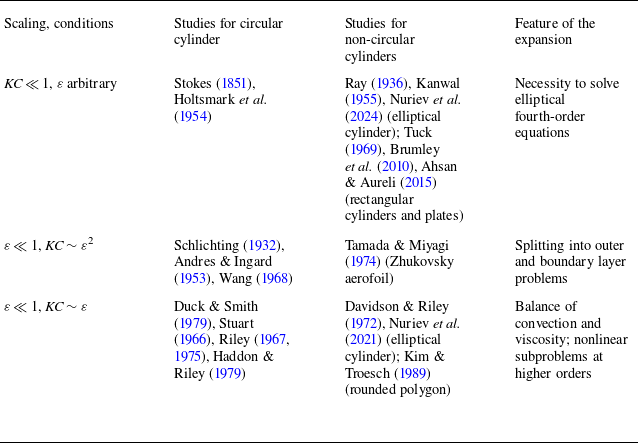
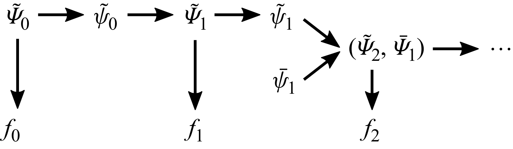
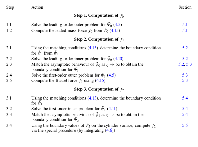
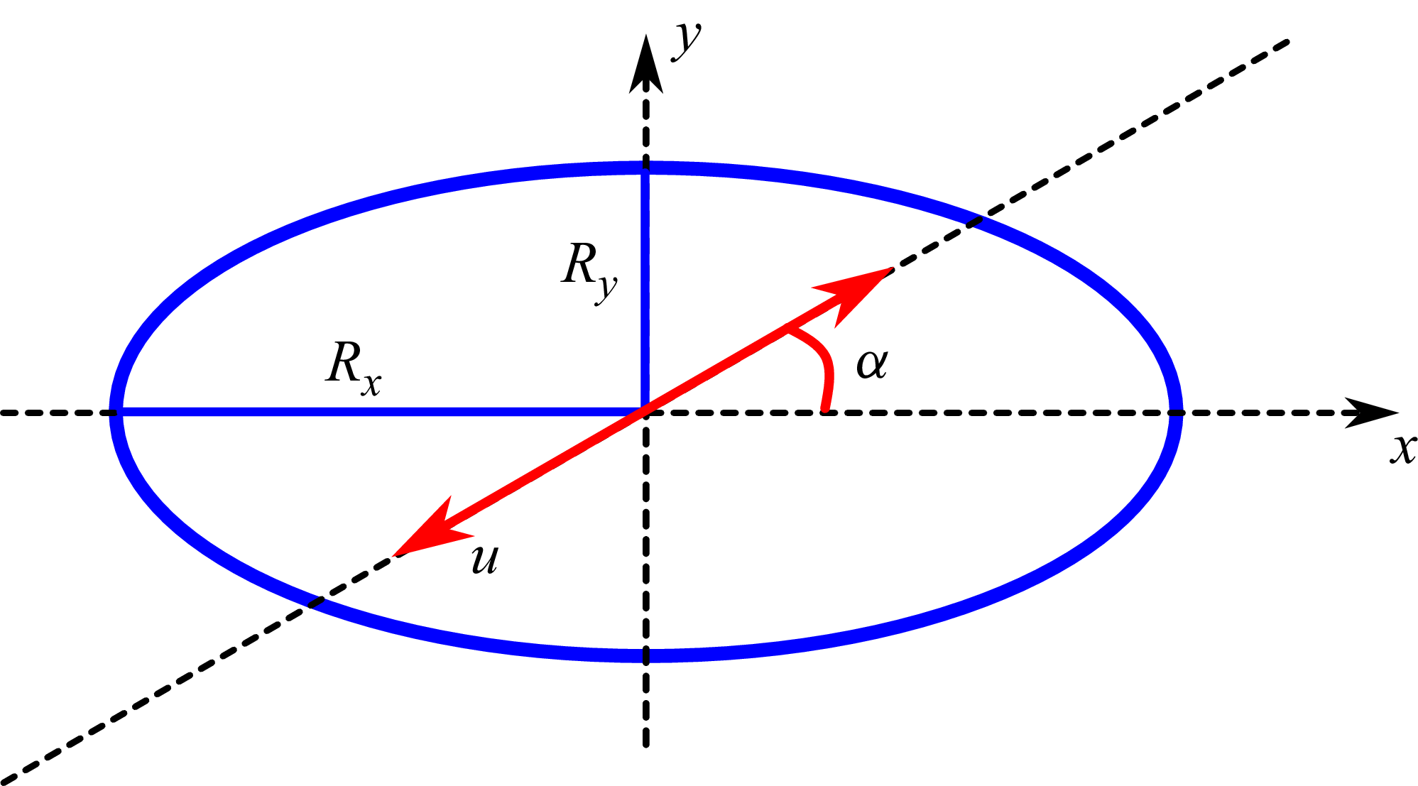

 CM
 CD
 b
 β=200
 KC=0.1,0.2
 α=π/2

 CD
 CM
 α=0
 β=200
 b
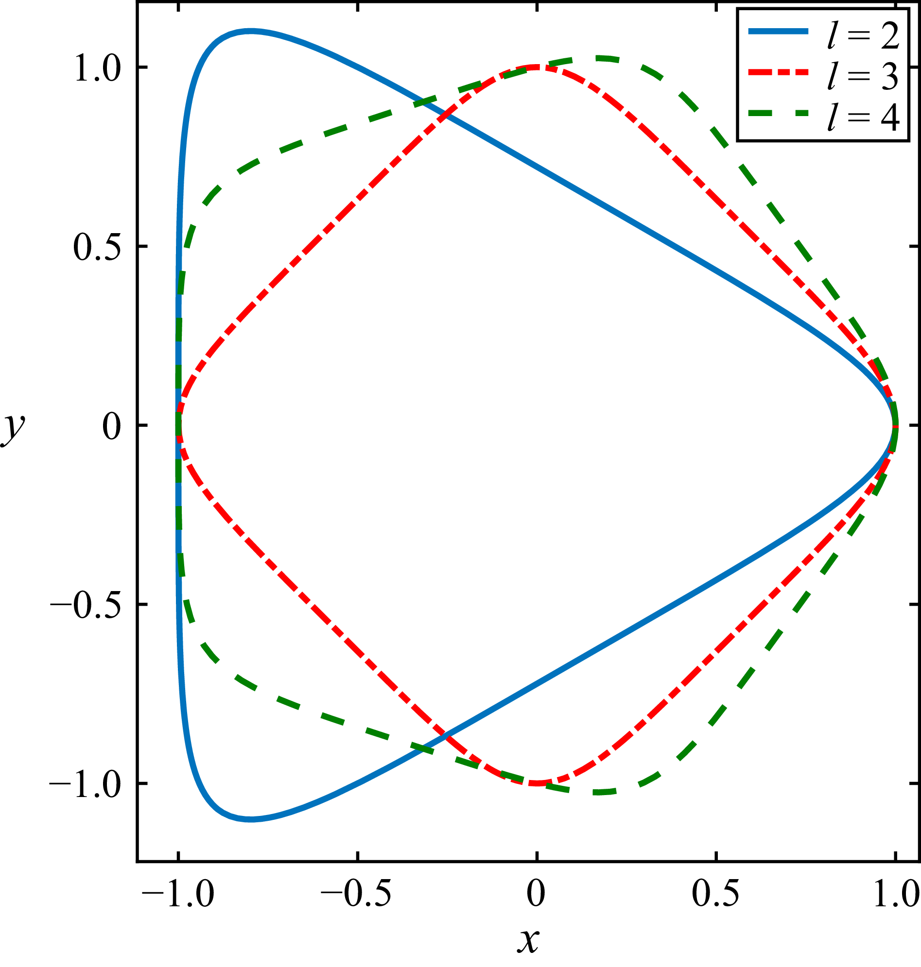
 c=l−2

 CD
 CM
 KC
 ε=0.056
 (β=200)
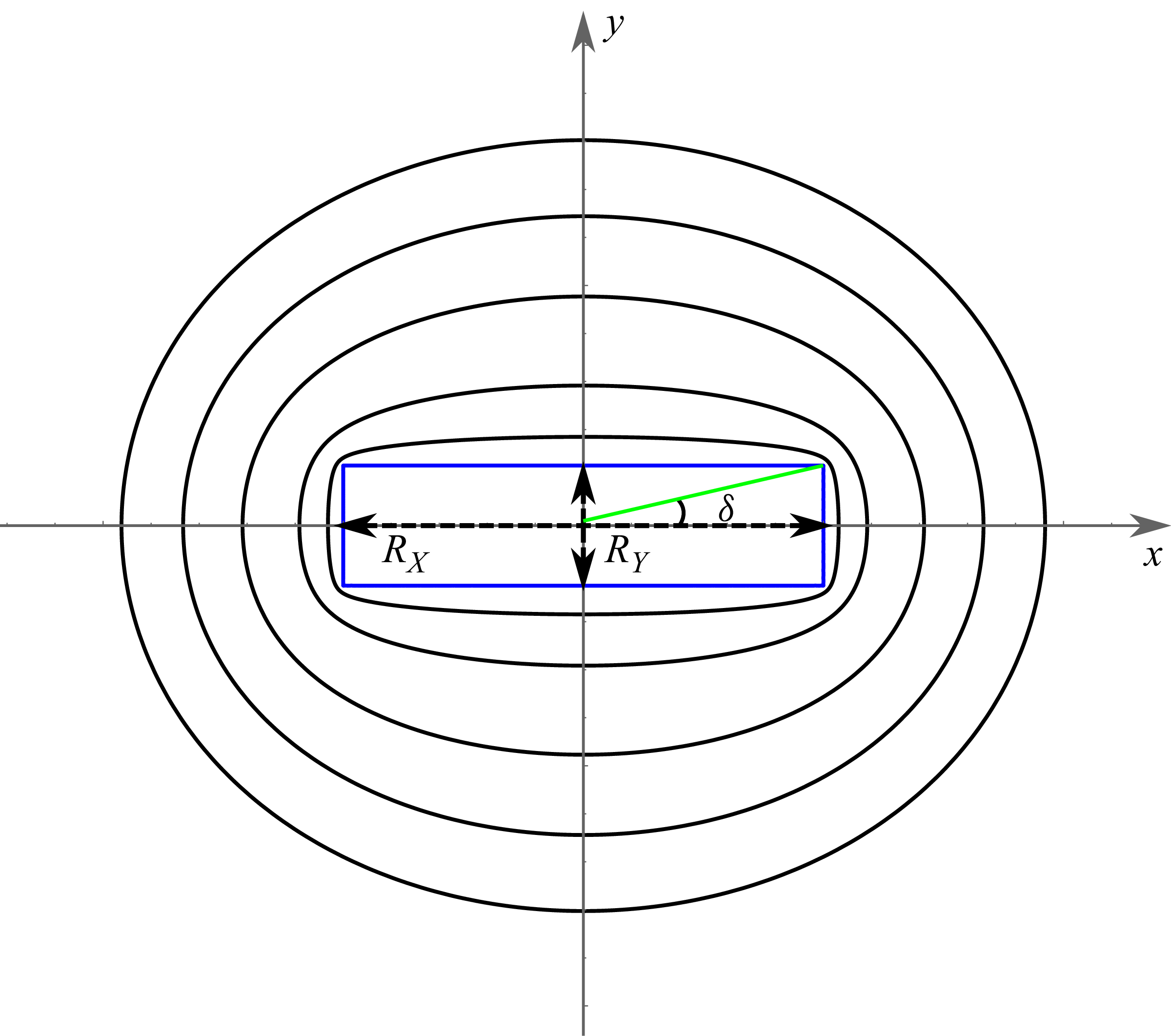
 r0=0
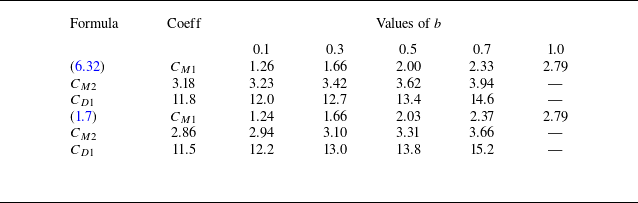
 CM1
 CM2
 CD1
 b

 CD
 α=π/2
 β=200
 b
 b=0.1
 β

 m
 m=0.5
 r0
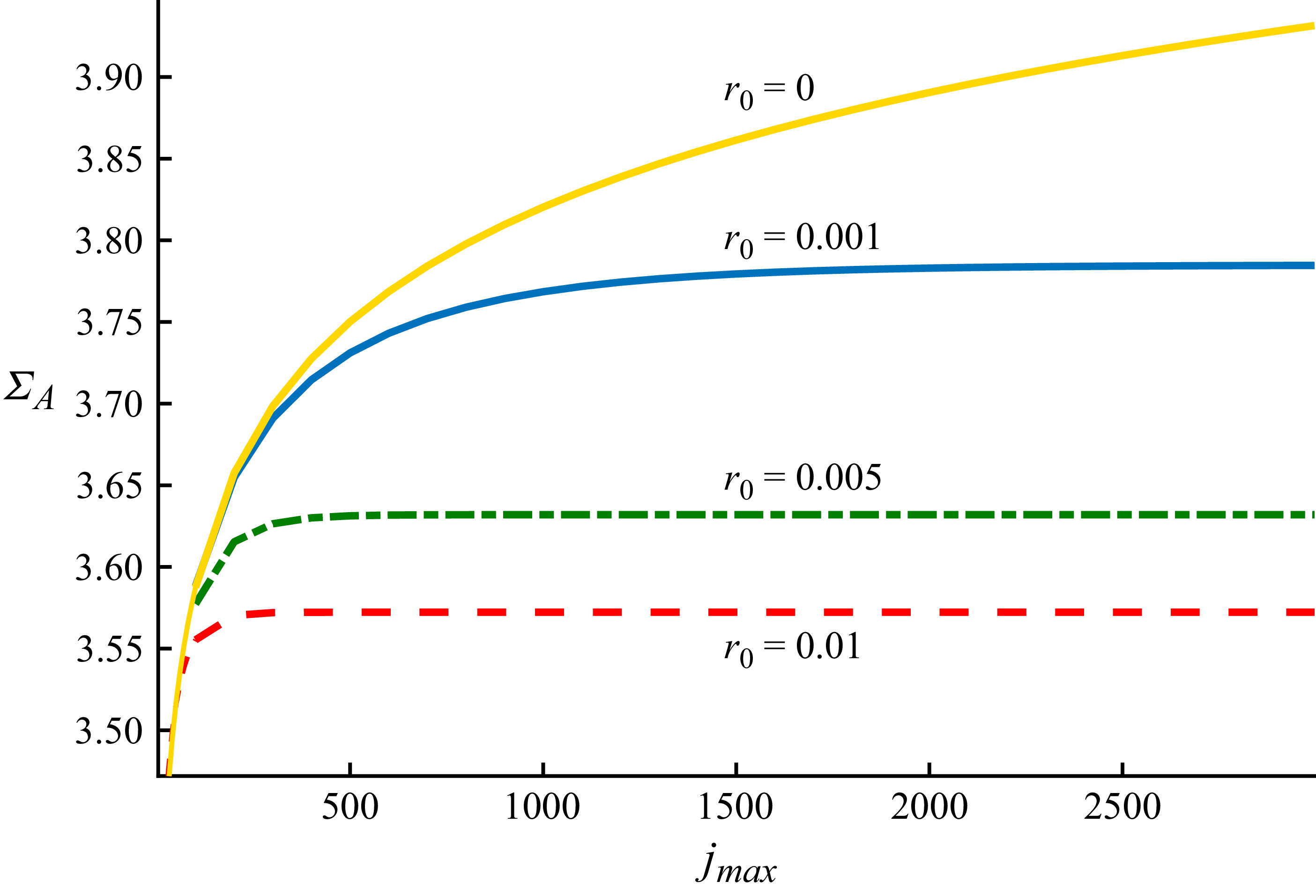
 ΣA
 m=1/2
 jmax
 r0

 CD
 CM
 KC
 β=400
 m=1/2
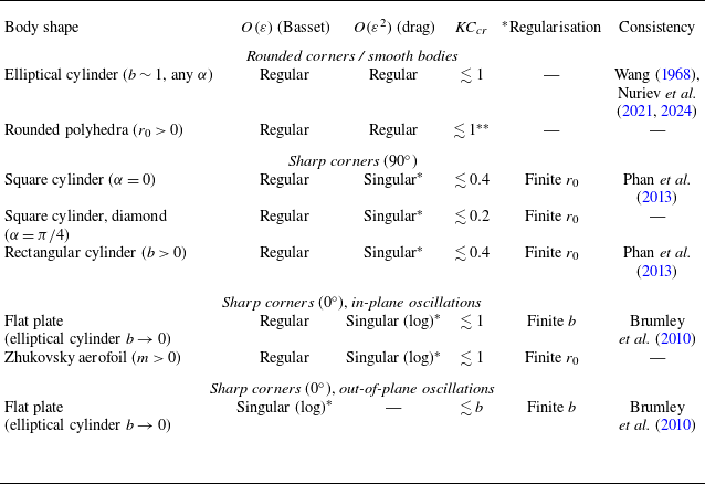
 O(1)
 KCcr
 CD
 CM
 KC
 ≲3
 ∗
 r0→0
 b→0
 r0
 b
 ∗∗


