1. Introduction
Shock reflection is a critical physical phenomenon, widely observed in both internal and external flow fields of aircraft. For supersonic aircraft engines, shock reflection is present at the lip of the inlet (Häberle & Gülhan Reference Häberle and Gülhan2007; Xie et al. Reference Xie, Wu, Yu and Guo2018; Sun et al. Reference Sun, Zhang, Ma and Xue2024; Tang et al. Reference Tang, Cai, Liu, Huang, Qin, Wang, Tan and Tian2025b ), within the internal flow (Onofri & Nasuti Reference von Neumann1999; Huang et al. Reference Huang, Wu, Yang, Yan and Li2020; Wu et al. Reference Wu, Xue, Ma, Li, Hou, Jiao, Cheng and Wang2025) and in the jet downstream of the nozzle exit (Powell Reference Powell1953; Arun Kumar & Rajesh Reference Arun Kumar and Rajesh2017; Li et al. Reference Li, He, Zhang, Hao, Wu and Liu2024); by changing flow field parameters, it affects the engine’s performance and efficiency. Therefore, a deeper understanding of shock reflection will contribute to the design of higher-performance engines.
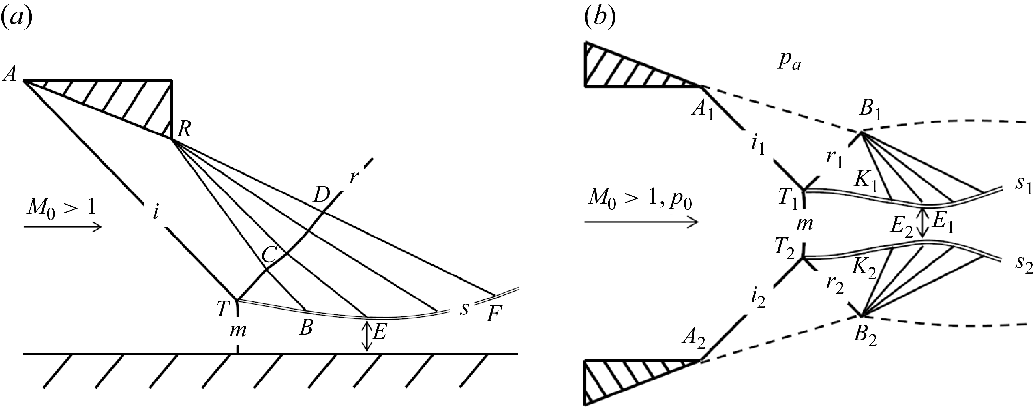
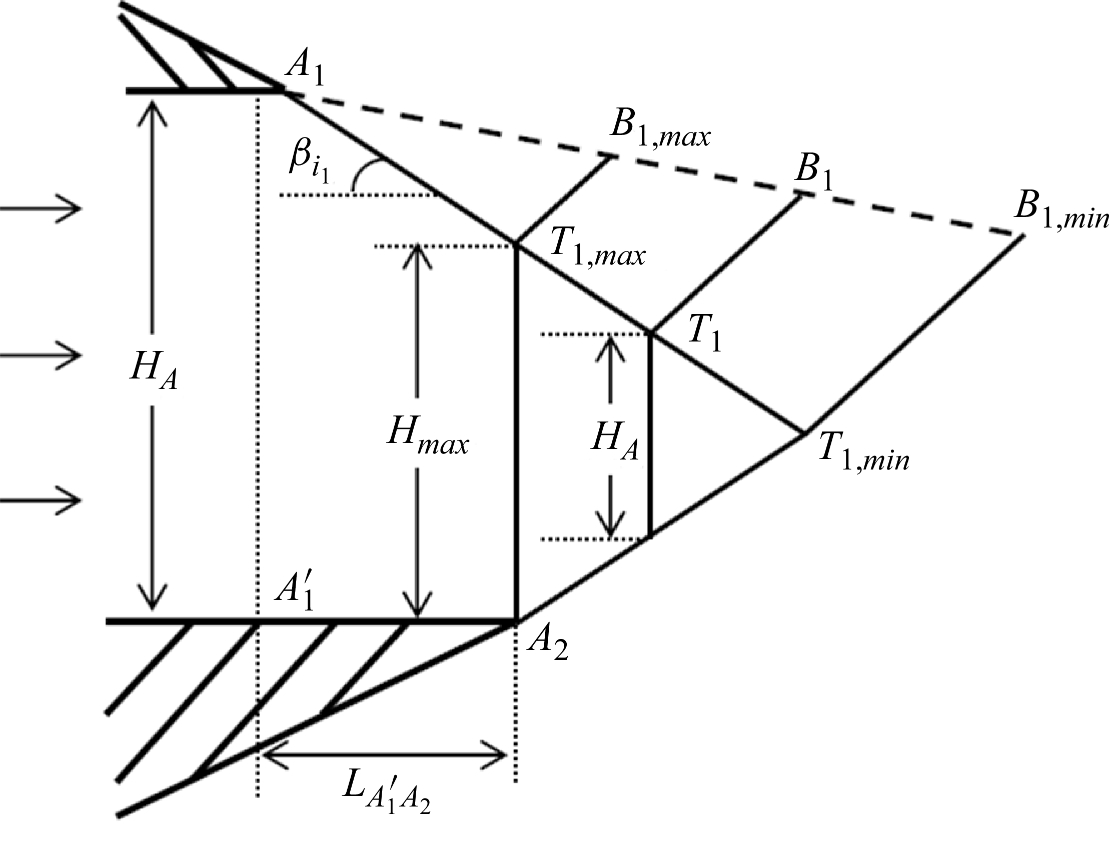
Two typical flow field structures of shock reflection are shown in figure 1. Figure 1(a) presents the shock reflection flow field structures of the incident shock generated by the wedge surface (wedge flow shock reflection) and figure 1(b) shows the shock reflection flow field structures of the incident shock caused by high ambient pressure (overexpanded jet shock reflection) (Hadjadj, Kudryavtsev & Ivanov Reference Häberle and Gülhan2004; Wu et al. Reference Wu, Xue, Ma, Li, Hou, Jiao, Cheng and Wang2025).
Schematic illustration of shock reflection. (a) Wedge flow shock reflection. (b) Overexpanded jet shock reflection. Here, i represents incident shock, r represents reflected shock, s represents slipline and m represents Mach stem.

For wedge flow shock reflection, the research on flow structures is relatively well established. Classical studies include shock reflection types (regular reflection (RR) and Mach reflection (MR) (Mach Reference Mach1878)), the triple-shock theory for the solution of flow parameters near the triple point (von Neumann Reference von Neumann1945), critical conditions (detachment criterion and von Neumann criterion (von Neumann Reference von Neumann1943)) and hysteresis phenomena (Henderson & Lozzi Reference Henderson and Lozzi1975; Hornung, Oertel & Sandeman Reference Hornung, Oertel and Sandeman1979; Vuillon, Zeitoun & Ben-Dor Reference Vuillon, Zeitoun and Ben-Dor1995; Ivanov et al. Reference Ivanov, Vandromme, Fomin, Kudryavtsev, Hadjadj and Khotyanovsky2001; Ben-Dor et al. Reference Ben-Dor, Ivanov, Vasilev and Elperin2002). In addition, scholars have also conducted detailed discussions on the multiple incident shock reflections (Ben-Dor, Dewey & Takayama Reference Ben-Dor, Dewey and Takayama1987; Guan et al. Reference Guan, Bai and Wu2018, Reference Guan, Bai, Lin and Wu2020; Meng et al. Reference Meng, Han, Yuan, Wang and Jiang2017; Li & Bai Reference Li, He, Zhang, Hao, Wu and Liu2025), curved shock reflection (Shi et al. Reference Shi, You, Zheng and Zhu2023; Zhang et al. Reference Zhang, Xu, Shi, Zhu and You2023; Yan et al. Reference Yan, Han, Xiong, Shi and You2024; Tian Reference Tian2024) and the shock reflection in axisymmetric flow (Ji et al. Reference Ji, Li, Zhang and Yang2019; Zhang et al. Reference Zhang, Hu, Da, Shi, Zhu and You2024; Shoesmith & Timofeev Reference Shoesmith and Timofeev2025). The influence of trailing edge height on Mach stem height (Bai & Wu Reference Bai and Wu2021), centred compression wave reflection (Bai Reference Bai2024), strong Mach reflection (Qin et al. Reference Qin, Shi, Dowell, Pei and Huang2022), the Mach reflection when the expansion wave at the wedge tail disturbs the incident shock wave (Bai Reference Bai2023), shock reflection over curved wedge (Wang et al. Reference Wang, Zhai, Luo, Yang and Lu2017, Reference Wang, Zhai and Luo2021, Reference Wang, Zhai and Luo2022), and interaction between centred-compression waves and cowl shock (Tang et al. Reference Tang, Cai, Huang, Tan, Qin and Tian2025a ) have also been studied.
For symmetric wedge flow shock reflection, an analytical solution model for flow field structures is a significant research focus. The commonality of the solution is that they all use classical quasi-one-dimensional flow theory to analyse the flow below the slipline. The model of Azevedo & Liu (Reference Azevedo and Liu1993) assumed that the sonic throat is located at the turning point (B in figure 1 a) where the slipline is disturbed/undisturbed by the leading characteristics line. The model of Li & Ben-Dor (Reference Li, He, Zhang, Hao, Wu and Liu1997a ) allowed the sonic throat to be determined by the transmitted expansion wave, using the assumption that the flow just above the sonic throat is parallel to the free stream flow. The model of Mouton & Hornung (Reference Mouton and Hornung2007) assumed that the sonic throat occurs further downstream and also assumed that the slipline is a straight line. Gao & Wu (Reference Gao and Wu2010) and Bai & Wu (Reference Bai and Wu2017) considered the secondary expansion waves generated on the initial segment of the slipline (TB in figure 1 a) due to the pressure drop caused by the contraction of the quasi-one-dimensional isentropic flow region. In general, the differences among these models lie in the localisation of the sonic throat, assumptions about the slipline shape and consideration of secondary flow field interference. Early models mostly relied on simplified assumptions (e.g. treating the slipline as a straight line and fixing the sonic throat at a specific position), while subsequent studies gradually incorporated practical flow effects such as secondary expansion waves induced by the contraction of the quasi-one-dimensional flow field, making the models more consistent with the complex physical nature and continuously improving prediction accuracy.
For asymmetric wedge flow shock reflection, an analytical solution model for flow field structures remains a significant research focus. Tao et al. (Reference Tao, Liu, Fan, Xiong, Yu and Sun2017) modelled the incident shock, reflected shock and Mach stem as straight lines, and the average flow deflection angle in the quasi-one-dimensional isentropic region as the mean of the upper and lower slipline angles – a value updated iteratively during the solution process. By incorporating the Prandtl–Meyer relation, they solved for the Mach stem height in asymmetric Mach reflection. Roy & Rajesh (Reference Roy and Rajesh2017) proposed a model that assumed the Mach stem to be a second-order curve and introduced a common horizontal symmetry axis within the quasi-one-dimensional isentropic flow region. By decomposing the asymmetric configuration into upper and lower symmetric subdomains, the model enabled the solution of asymmetric Mach reflection. Building upon this work, Roy & Gopalapillai (Reference Roy and Gopalapillai2019) further introduced the concept of the average flow deflection angle, defined as the mean of the streamline deflection angles induced by the Mach stem at the upper and lower triple points, which extended the model’s capability to predict inverse Mach reflection (InMR) configurations. Additionally, such assumption of the average flow deflection angle in the quasi-one-dimensional isentropic flow region was similarly employed by Lin, Bai & Wu (Reference Lin, Bai and Wu2019). They hypothesised the Mach stem as a circular arc, and by incorporating interactions between secondary waves and the sliplines, they systematically analysed the effects of asymmetric upper and lower wedge angles, wedge lengths, and streamwise leading-edge positions on the flow field structures.
For overexpanded jet shock reflection, the reflection types, critical criteria and hysteresis phenomena are consistent with those of the wedge flow shock reflection. Their difference lies in the flow field structure. When the incident shocks are caused by high ambient pressure, the reflected expansion waves (at
 $B_1 \,\text{and}\, B_2$
in figure 1
b) do not interfere with the reflected shocks (
 $T_1B_1 \,\text{and}\, T_2B_2$
in figure 1
b), but directly interact with the sliplines. In addition, scholars have also conducted discussions on the hysteresis phenomenon in jet flows by experiments (Kashitani et al. Reference Kashitani, Yamaguchi, Miyazato, Masuda and Matsuo2003; Matsuo et al. Reference Matsuo, Setoguchi, Nagao, Alam and Kim2011; Lavala & Das Reference Lavala and Das2025) and CFD (computational fluid dynamics) simulations (Hadjadj et al. Reference Häberle and Gülhan2004; Yasunobu et al. Reference Yasunobu, Matsuoka, Kashimura, Matsuo and Setoguchi2006; Shimshi et al. Reference Shimshi, Ben-Dor and Levy2009, Reference Shimshi, Ben-Dor and Levy2015; Hew, Ogawa & Boswell Reference Hew, Ogawa and Boswell2024).
For symmetric overexpanded jet shock reflection, the analytical solution model for flow field structures is relatively well established. When considering the non-uniformity of the flow field downstream of the incident and reflected shock, the method of characteristics (MOC) can be used to establish a model for solving the flow field structures of overexpanded jet. The earliest relevant work was carried out by Ashratov (Reference Ashratov1966). Subsequently, Chow & Chang (Reference Chow and Chang1975) extended the solution to the case where the region downstream of the reflected shock is subsonic. Rolland et al. (Reference Rolland, Shoesmith and Timofeev2024) considered a more refined flow field downstream of the incident shock to solve the Mach stem height, enhancing the prediction accuracy for small Mach stems. When considering the uniformity of the flow field downstream of the incident and reflected shock, predictive models for flow field structures are also established in an overexpanded jet. Li & Ben-Dor (Reference Li, He, Zhang, Hao, Wu and Liu1997b ) incorporated the effects of expansion waves on the jet structure. The straight lines assumption is used to model the incident shock wave, reflected shock wave, jet boundary and the part of the slipline not intersecting with the expansion wave. Additionally, the part of the slipline intersecting with the expansion wave is modelled as a curve with a small curvature. From this, they derived a theoretical predictive model for the flow field structures and size. Omelchenko, Uskov & Chernyshov (Reference von Neumann2003) investigated the interaction between the reflected shock and secondary expansion waves, predicting the Mach stem height in an overexpanded jet using an iterative approach with termination conditions based on either achieving sonic flow or flow flattening at the throat. Chernyshov, Savelova & Kapralova (Reference Chernyshov, Savelova and Kapralova2021) extended the model proposed by Omelchenko et al. (Reference von Neumann2003), described expansion waves based on the straight-line assumption and developed a theoretical model for the rapid prediction of the flow field structures of Mach reflection in an overexpanded jet based on flow averaging downstream of a curved Mach stem. Based on the classical shock reflection models of Li & Ben-Dor (Reference Li, He, Zhang, Hao, Wu and Liu1997a ), Mouton & Hornung (Reference Mouton and Hornung2007) and Bai & Wu (Reference Bai and Wu2017). Paramanantham, Janakiram & Gopalapillai (Reference Paramanantham, Janakiram and Gopalapillai2022) provided three revised models to solve the flow field configuration in an overexpanded supersonic jet. They also compared these revised models with experimental and numerical results to verify their validity.
For asymmetric overexpanded jet shock reflection, frequently induced by non-ideal engineering conditions, current research remains relatively insufficient. Upstream non-uniformity-induced asymmetric flow structures represent one of the key contributing factors. This issue has been preliminarily explored by Hew et al. (Reference Hew, Boswell, Federrath, Gopalapillai and Paramanantham2023), who introduced Mach number non-uniformity at the inlet to solve the flow field structure of asymmetric Mach reflection. Another crucial factor is nozzle exit geometric asymmetry, which represents a common and important engineering scenario. Such geometric asymmetries may originate from numerous engineering factors: manufacturing tolerances leading to actual lip position deviations, active asymmetric designs in thrust vectoring nozzles (Lv et al. Reference Lv, Xu, Yu and Mo2017), etc. The above-mentioned factors lead to differences in the upper and lower shock positions of the jet, thereby inducing asymmetric shock reflection. Compared with symmetric shock reflection, the throat flow deflects and the expansion wave interactions on both sides of the throat need to be considered in a coupled manner. However, a systematic theoretical modelling study on this issue is still lacking.
In general, research on the asymmetric overexpanded jet shock reflection remains relatively limited. This paper develops a theoretical model that can predict the asymmetric flow field structures in a supersonic overexpanded jet. The structure of this paper is as follows: § 2 defines the the physical scenario of asymmetric flow in an overexpanded jet, describes the numerical methods employed and analyses the flow field of asymmetric supersonic overexpanded jet with numerical results; § 3 presents the theoretical model used in this article; § 4 evaluates the theoretical model’s accuracy and studies the influence of nozzle exit parameters of flow field structures; and § 5 summarises the main conclusions.
2. Numerical simulation method and flow characteristics of asymmetric shock reflection in an overexpanded jet
In this section, we first define the physical scenario of asymmetric flow in an overexpanded jet caused by nozzle geometric asymmetry. Then, we present the CFD method used here. Finally, we analyse the flow characteristics in asymmetric shock reflection in an overexpanded jet based on CFD results. In this paper, the specific-heat ratio
 $\gamma$
is 1.4 and the gas constant R is 287 J (kg K)−1.
2.1. Definition of asymmetric shock reflection in an overexpanded jet
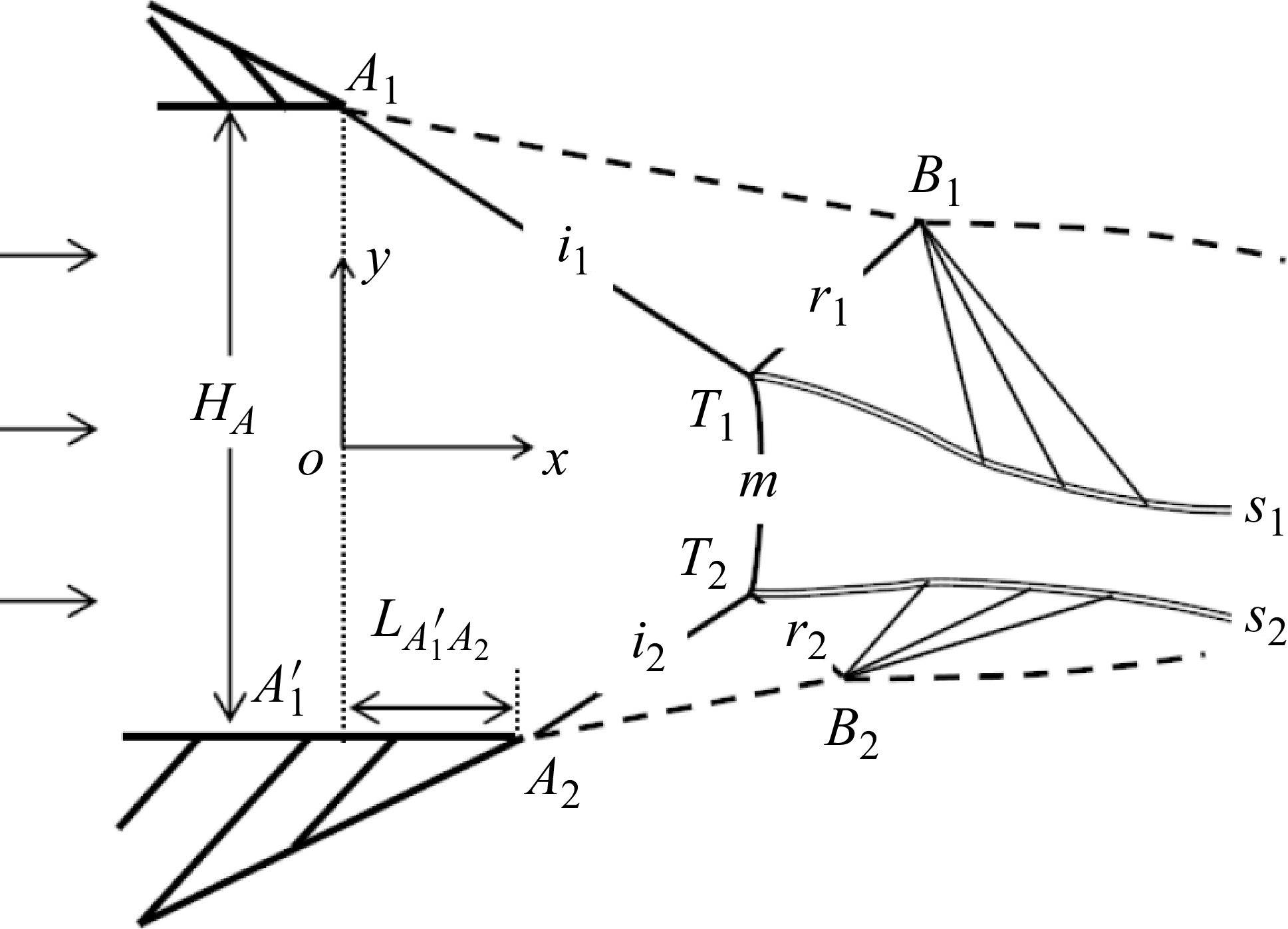
Figure 2 is a schematic illustration of asymmetric Mach reflection in an overexpanded jet. The shaded triangles represent nozzle exit geometry, where the exit velocity is aligned with the x-axis. The nozzle height
 $A_{1}A_{1}'$
is
 $H_{A}$
, nozzle exit Mach number is
 $M_{0}$
and nozzle pressure ratio (NPR) is denoted as the ratio of the stagnation chamber pressure to the ambient pressure. The asymmetry originates from the offset in x-coordinates between upper and lower nozzles. To quantitatively analyse this asymmetry, we define a dimensionless form of the extension length of the lower nozzle (
 $A'_{1}A_{2}$
in figure 2) as
 \begin{align} L_w=\frac {L_{A'_{1}A_{2}}}{H_A}. \end{align}
When
 $L_w \neq 0$
, expansion waves reflected at the lower jet boundary interact with the slipline first, causing flow deflection downward and resulting in an asymmetric overexpanded jet.
Schematic illustration of asymmetric Mach reflection in an overexpanded jet.

Moreover, it is evident that
 $L_w$
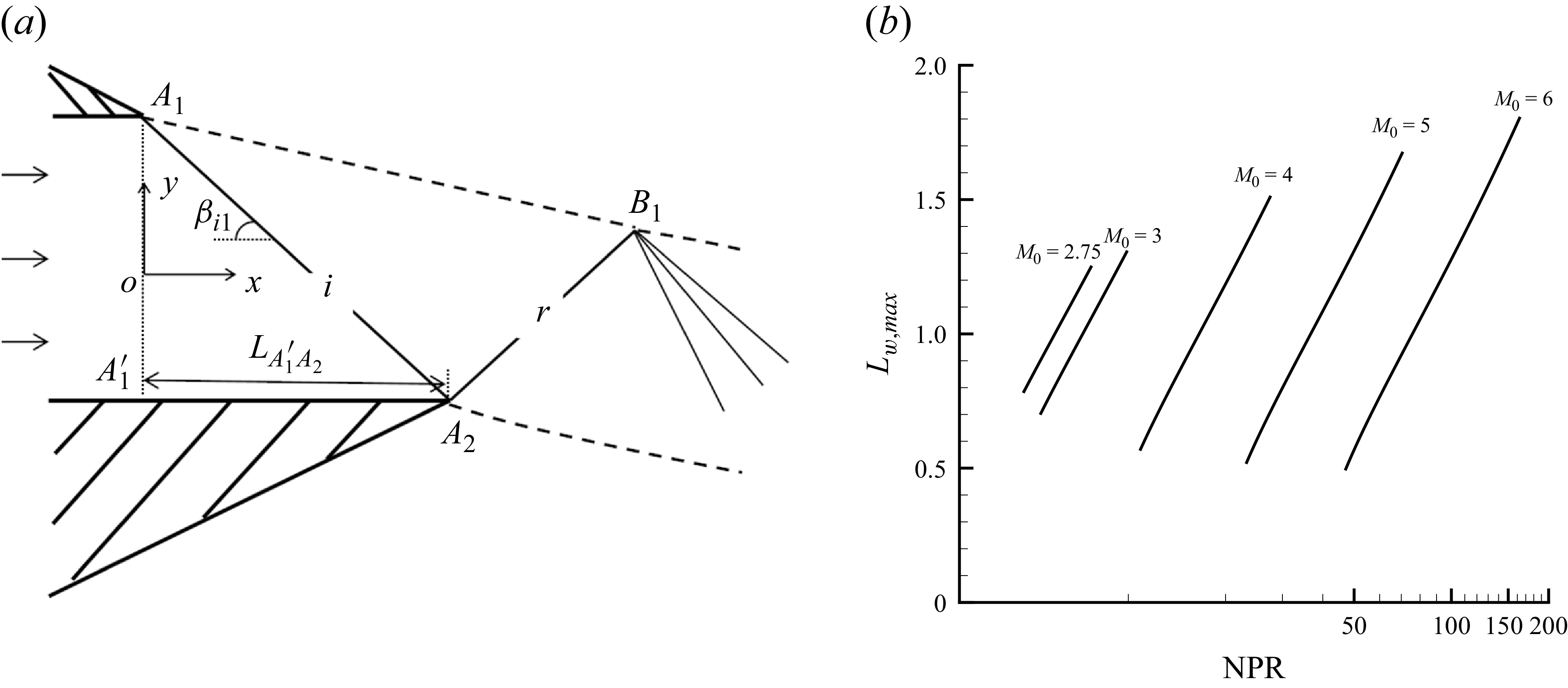
cannot increase indefinitely. As shown in figure 3(a), when the extension line of the incident shock wave at the upper lip position
 $A_{1}$
intersects precisely with
 $A'_{1}A_{2}$
, the asymmetric shock reflection does not exist. Denoting the corresponding
 $L_{w}$
as
 $L_{w, \textit{max}}$
,
 \begin{align} L_{w, \textit{max}}=\frac {1}{\tan \beta _{i1}} ,\end{align}
where
 $\beta _{i1}$
is the shock angle of the upper incident shock wave, which can be calculated using the classical oblique shock relations.
Flow structure and its predictive parameter under
 $L_{w, \textit{max}}$
. (a) Schematic illustration of flow structure corresponding to
 $L_{w, \textit{max}}$
. (b) Variation of the predictive
 $L_{w, \textit{max}}$
at different NPR when given
 $M_{0}$
.

Given NPR, ambient pressure and
 $M_{0}$
,
 $p_{0}$
can be obtained via the stagnation pressure–static pressure relation for isentropic flow. Then,
 $\beta _{i1}$
can be obtained using oblique shock relations. From (2.2), the variation of
 $L_{w, \textit{max}}$
with NPR under different Mach numbers is derived, as shown in figure 3(b). Here,
 $L_{w, \textit{max}}$
increases with the increase of NPR and decreases with the increase of Mach number.
2.2. Numerical simulation method
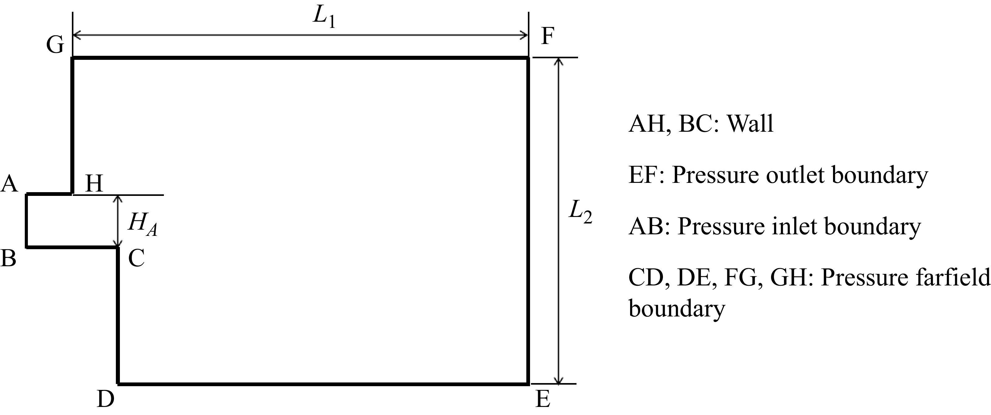
The boundary conditions are illustrated in figure 4, where AH, BC are set as the wall, AB is set as the pressure inlet, EF is set as the pressure outlet, and CD, DE, FG, GH are set as the pressure far field. To facilitate subsequent verification of the computational domain independence, the dimensions of the computational domain are defined as
 $L_{1}$
and
 $L_{2}$
.
Boundary condition for CFD calculation.

We solve the full set of nonlinear Euler equations in gas dynamics using the well-known Roe scheme based on the finite difference approximation and second-order upwinding for the flux. The solution is considered converged when the size and shape of the Mach stem remain unchanged after sufficient iterations. A structured grid is adopted, with refinement applied to regions featuring complex flow structures. It is assumed that the gas flows uniformly from the nozzle in the form of an inviscid ideal gas and the parameters conform to the isentropic flow relationship.
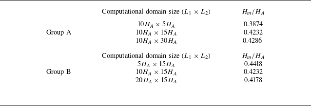
We first conduct domain size independence. Table 1 presents the Mach stem height of different domain size for the condition
 $M_{0}=3$
,
 $ \textit{NPR}=7$
and
 $L_{w}=0$
. Group A analyses the effects of the computational domain dimensions perpendicular to the flow direction (
 $L_{1}$
). When replacing the computational domain size from
 $10H_A\times 30H_A$
to
 $10H_A\times 15H_A$
, the Mach stem height decreases by only 1.26 %. Group B analyses the effects of the computational domain dimensions along the flow direction (
 $L_{2}$
). When changing from
 $20H_A\times 15H_A$
to
 $10H_A\times 15H_A$
, the increase is merely 1.29 %. Therefore, based on a consideration of accuracy and computational efficiency,
 $L_{1}$
is set as
 $10H_A$
and
 $L_{2}$
is set as
 $15H_A$
for subsequent computations.
Computational domain size independence test results for
 $M_{0}=3,\, \mathrm{NPR}=7,\, L_{w}=0$
.

Then, we conduct the grid density independence test. Table 2 presents the different grid configurations and corresponding Mach stem height for the condition
 $M_{0}=3$
,
 $\textit{NPR}=9$
and
 $L_{w}=0$
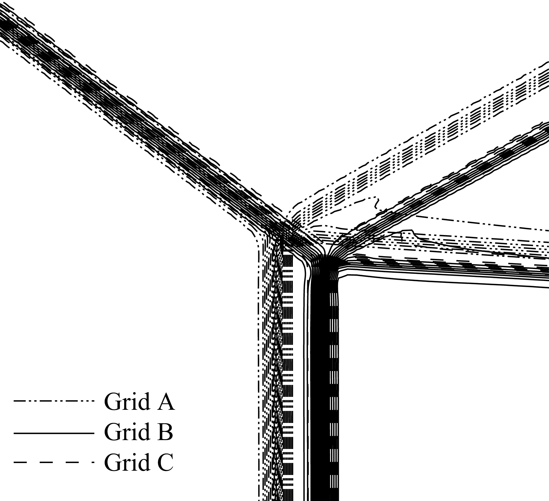
. The number of grid nodes distributed along the Mach stem is N. When replacing the grid from Grid C with Grid B, the Mach stem height difference is only 1.85 %. Moreover, figure 5 comparatively displays the Mach number contours near the triple point. The dash–dot–dotted lines, solid lines and dashed lines represent the computational results for Grid A, Grid B and Grid C, respectively. The Mach number contours of Grid B and Grid C are essentially identical. Thus, we conclude that a minimum of 150 grid points must be distributed along the Mach stem to ensure sufficient accuracy of numerical results.
Grid configurations and computational domain size independence test results for
 $M_{0}=3, \,\mathrm{NPR}=9,\, L_{w}=0$
. N represents the grid number along the Mach stem.

CFD simulation results: Mach number contours of overexpanded jet near the upper triple point under
 $M_{0}=3$
, NPR = 9,
 $L_{w}$
= 0.

In summary, the grid used in this study is characterised by a computational domain size of
 $10H_A\times 15H_A$
, with at least 150 grid points guaranteed in the height direction of the Mach stem and a uniformly graded transition adopted in other regions.
2.3. Analysis of flow structures of asymmetric shock reflection in overexpanded jet
Figure 6(a) shows the CFD results for an asymmetric shock reflection under
 $M_{0}=3$
, NPR = 11,
 $L_{w}=0.1$
. The NPR exceeds the von Neumann criterion (von Neumann Reference von Neumann1943), resulting in an asymmetric regular reflection. Two incident shocks
 $A_{1}T$
and
 $A_{2}T$
form at the lip. These two opposite-side incident shocks reflect as two reflected shocks
 $B_{1}T$
and
 $B_{2}T$
. The reflected shocks interact with the jet boundaries
 $A_{1}B_{1}$
and
 $A_{2}B_{2}$
, generating two Prandtl–Meyer expansion waves.
CFD simulation results: Mach number contours (grey solid lines) and characteristic lines (black solid lines) of asymmetric overexpanded jet under
 $L_{w}=0.1$
. (a)
 $M_{0}=3$
, NPR = 11. (b)
 $M_{0}=3$
, NPR = 7.

Figure 6(b) shows the CFD results for an asymmetric shock reflection under
 $M_{0}=3$
, NPR = 7,
 $L_{w}=0.1$
. The NPR is in dual solution domain (von Neumann Reference von Neumann1943), resulting in an asymmetric Mach reflection. Two incident shocks
 $A_{1}T_{1}$
and
 $A_{2}T_{2}$
are connected by a Mach stem
 $T_{1}T_{2}$
. At the triple points
 $T_{1}$
and
 $T_{2}$
, two incident shocks reflect as two reflected shocks
 $B_{1}T_{1}$
and
 $B_{2}T_{2}$
. The region downstream of the Mach stem is initially subsonic and then gradually becomes supersonic, and can be divided into three regions based on whether there is interference from upper/lower reflected expansion waves. Initially, neither the upper nor lower expansion waves interfere with the region downstream of the Mach stem. Subsequently, the lower expansion wave first interferes with the downstream region of the Mach stem. Finally, both the upper and lower expansion waves interfere with the downstream region of the Mach stem. Moreover, the sonic locations
 $E_{1}$
and
 $E_{2}$
, and the points of flow horizontalisation are displayed and their positions do not coincide.
3. Theoretical model for asymmetric shock reflection in an overexpanded jet
In this section, a theoretical model for predicting flow field structures in an asymmetric shock reflection in an overexpanded jet is established. The theoretical model aims to describe the shape, position and dimensions of the flow field structures – including the incident shocks, reflected shocks and sliplines for given nozzle exit parameters.
3.1. Theoretical model of asymmetric shock reflection in an overexpanded jet
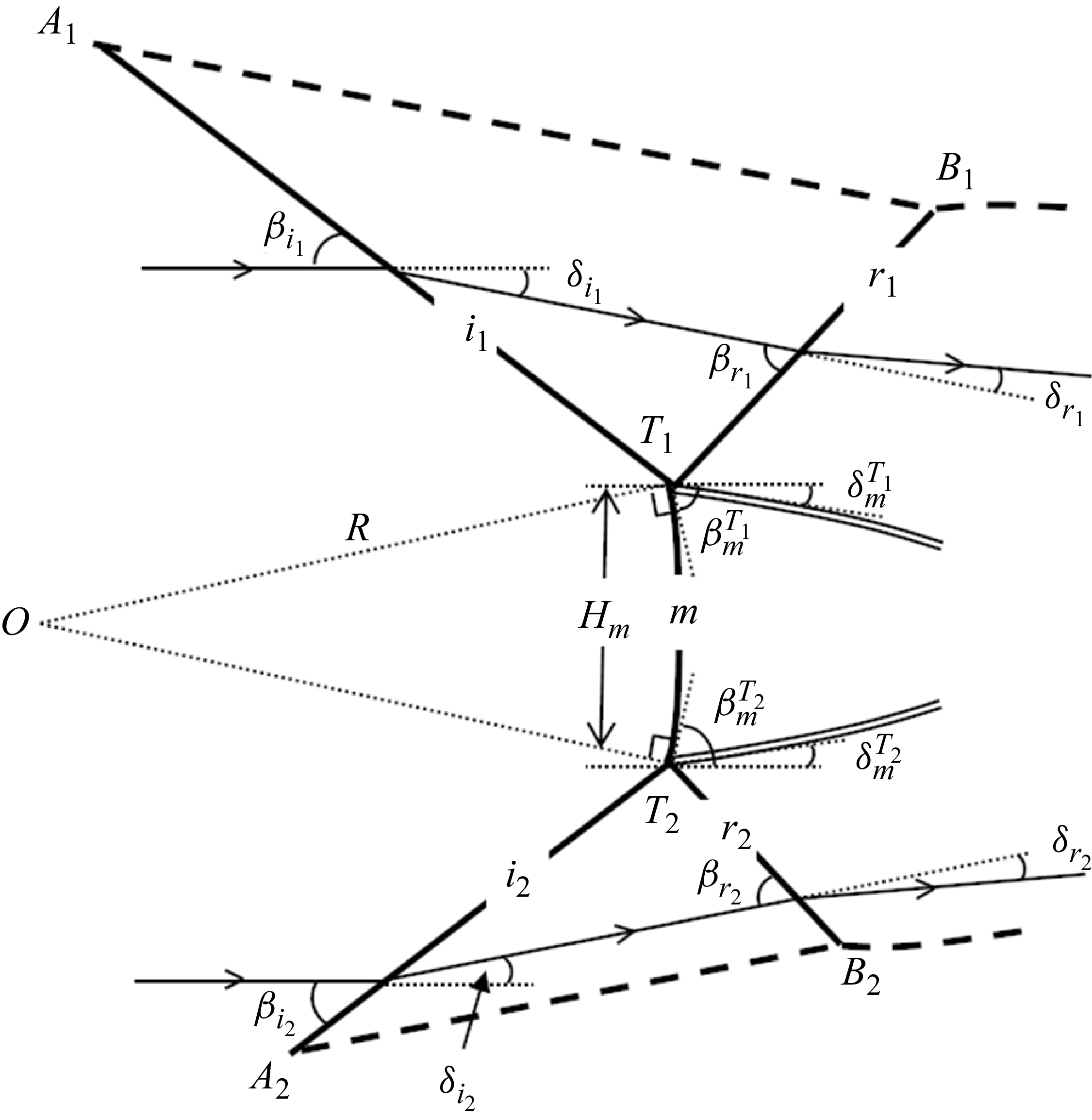
Figure 7 is the schematic illustration of asymmetric Mach reflection in an overexpanded jet. The flow is divided into seven regions: region (0) is upstream of the Mach stem and two incident shock waves; region (1) is between the incident shock wave
 $i_{1}$
and the reflected shock wave
 $r_{1}$
; region (2) is between the reflected shock wave
 $r_{1}$
and the expansion wave reflected at point
 $B_{1}$
; region (3) is downstream of the Mach stem; region (4) is the region of expansion wave reflected at point
 $B_{1}$
; region (5) is between the incident shock wave
 $i_{2}$
and the reflected shock wave
 $r_{2}$
; region (6) is between the reflected shock wave
 $r_{2}$
and the expansion wave reflected at point
 $B_{2}$
; and region (7) is the region of the expansion wave reflected at point
 $B_{2}$
.
Schematic illustration of asymmetric Mach reflection in an overexpanded jet.

Slipline
 $s_{1}$
and slipline
 $s_{2}$
are the upper slipline and lower slipline, respectively. Here,
 $\delta _{s_1}$
and
 $\delta _{s_2}$
are respectively the upper slipline deflection angle and the lower slipline deflection angle, and counterclockwise rotation from the positive x-axis is defined as positive here. There is a noticeable misalignment between the upper and lower interference segments of the sliplines. Therefore, when solving sliplines, the problem should be categorised into three cases: (i) both segments being free; (ii) one segment being free, while the other is an interference segment; and (iii) both segments being interference segments. Here,
 $H_{m}$
is the given Mach stem height. The height of the quasi-one-dimensional channel
 $H_{s}$
is the height of the quasi-one-dimensional isentropic channel perpendicular to the average flow direction of the throat. Specific expressions are provided in § 3.2.3. Additionally,
 $M_{s}$
and
 $p_{s}$
are the Mach number and pressure in region (3);
 $M _{s_1}$
and
 $p_{s_1}$
are the Mach number and pressure near the upper slipline
 $s_{1}$
in region (2) and region (4);
 $M _{s_2}$
and
 $p_{s_2}$
are the Mach number and pressure near the lower slipline
 $s_{2}$
in region (6) and region (7).
3.2. Analytical methods pertinent to flow field structures
3.2.1. Solution of the coordinates of triple points
The coordinates of triple points should be solved first as the initial coordinates of upper and lower sliplines. As discussed in § 2.3, there is no interaction between the reflected shock wave and the expansion waves reflected at the jet boundary in overexpanded jet shock reflection. The incident shock waves, reflected shock waves and jet boundaries are straight lines, while the Mach stem is an arc with a large radius. Therefore, the geometric relationships for the incident shock waves, reflected shock waves and Mach stem proposed by Lin et al. (Reference Lin, Bai and Wu2019) are used here.
The solution approach of coordinates of triple points is as follows: given the nozzle exit Mach number
 $M_{0}$
and NPR, the classical oblique shock wave relation and triple shock theory (von Neumann Reference von Neumann1945) can solve the flow parameters near the triple points. This allows the slopes of the incident shocks to be identified as −
 $\tan \beta _{i_1}$
and
 $\tan \beta _{i_2}$
, and the deflection angles of the Mach stem near the triple points to be −
 $ \delta _{m}^{T_1}$
and
 $ \delta _{m}^{T_2}$
. Next, the circular arc hypothesis of the Mach stem is introduced. Tan et al. (Reference Tan, Ren and Wu2006) have discussed the basic assumption that the Mach stem is a circular arc with a large radius, starting from the isentropic small-disturbance equations. Our theoretical model adopts this assumption for the solution. The triple points are assumed to lie on a circle centred at O with radius R. The slopes of
 $OT_1$
and
 $OT_2$
are
 $\tan ({\pi }/{2}-\beta ^{T_1}_{m})$
and
 $-\tan ({\pi }/{2}-\beta ^{T_2}_{m})$
, respectively. With the Mach stem height specified, the coordinates of the triple points
 $T_{1}\,\text{and}\,T_{2}$
can be determined. Subsequently, the coordinates of points
 $B_{1}\,\text{and}\,B_{2}$
can be calculated by solving the straight-line equations of the jet boundary and reflected shock. The detailed equations are shown in Appendix A.
3.2.2. Governing equations for slipline flow parameters
Section 2.3 describes the flow field characteristics associated with the free segments of sliplines (
 $T_{1}K_{1}$
and
 $T_{2}K_{2}$
in figure 7). Accompanied by the contraction of the one-dimensional isentropic flow region and the resulting pressure drop, secondary expansion waves are generated along the free segment of the slipline to maintain the pressure balance. These secondary waves further influence the slope of the slipline.
This mechanism was applied by Omelchenko et al. (Reference von Neumann2003) to Mach reflection in an overexpanded jet and by Gao & Wu (Reference Gao and Wu2010) to that in wedge flows, and was systematically discussed by Silnikov & Chernyshov (Reference Silnikov and Chernyshov2015), who further analysed the possible geometric shapes of the free segment and the interference segment of the slipline. Furthermore, Paramanantham et al. (Reference Paramanantham, Janakiram and Gopalapillai2022) also incorporated this mechanism in their modelling and analysis of shock reflection problems in symmetric jet flows. Furthermore, secondary waves have been accounted for by Bai & Wu (Reference Bai and Wu2017) and Paramanantham et al. (Reference Paramanantham, Janakiram and Gopalapillai2022).
Therefore, we can present the governing equations for flow parameters near slipline
 $s_{1}$
in the upper region (2):
 \begin{align} \left \{ \begin{aligned} &\nu \big(M_{s_1} \big)-\nu \big(M_{2}^{T_1}\big) =-\delta _{s_1}+\delta _{m}^{T_1},\\[6pt] &p_{s_1}=p_{2}^{T_1}\left(\frac {\vartheta \big(M_{2}^{T_1} \big)}{\vartheta \big(M_{s_1}\big)}\right)^{\frac {\gamma }{\gamma -1}},\\ \end{aligned} \right . \end{align}
where
 $M_{2}^{T_1}, p_{2}^{T_1}$
is the Mach number and pressure of the airflow in region (2) near the triple point
 $T_{1}$
;
 $\nu (M)$
is the Prandtl–Meyer relation and
 \begin{align} \left \{ \begin{aligned} &\vartheta (M)=1+\frac {\gamma -1}{2}M^2,\\[5pt]&\nu (M)=\sqrt {\frac {\gamma +1}{\gamma -1}}\arctan \sqrt {\frac {\gamma -1}{\gamma +1}(M^2-1)}-\arctan \sqrt {M^2-1}.\\ \end{aligned} \right . \end{align}
Additionally, the governing equations for flow parameters near slipline
 $s_{2}$
in region (6) are
 \begin{align} \left \{ \begin{aligned} &\nu \big(M_{s_2}\big)-\nu \big(M_{6}^{T_2}\big) = \delta _{s_2}-\delta _{m}^{T_2},\\[5pt]&p_{s_2}=p_{6}^{T_2} \left(\frac {\vartheta \big(M_{6}^{T_2}\big)}{\vartheta \big(M_{s_2}\big)}\right)^{\frac {\gamma }{\gamma -1}},\\ \end{aligned} \right . \end{align}
where
 $M_{6}^{T_2}, p_{6}^{T_2}$
are the Mach number and pressure of the airflow in region (6) near the triple point
 $T_{2}$
.
The flow characteristics of the interference segments of the sliplines (
 $K_{1}E_{1}$
and
 $K_{2}E_{2}$
in figure 7) are also described in § 2.3. The pressure drop resulting from the flow passing through the reflected expansion waves is the dominant factor driving the pressure change. To match this pressure drop, the quasi-one-dimensional isentropic flow region contracts, ultimately leading to a change in the curvature of the slipline.
In the solution for a symmetric jet, Paramanantham et al. (Reference Paramanantham, Janakiram and Gopalapillai2022) employed the straight-line assumption to describe the reflected expansion waves and solved for the interference segment of the slipline. In this study, we further assume the reflected expansion waves to be small-curvature curves, based on which the governing equations for flow parameters near the interference segments of the sliplines are established. This assumption aligns with the flow characteristics depicted in figure 6. The derivation of the governing equations for flow parameters in the slipline interference segments can refer to the methodology of Bai (Reference Bai2023), with the distinction that in this model, the expansion waves do not interact with the reflected shock waves.
The expressions for solving the small flow deflection increment
 $\mathrm{d}\theta _{B_1}$
at position
 $B_1$
in region (4) and the angular change
 $\mathrm{d}\delta _{s_1}$
of slipline
 $s_{1}$
are
 \begin{align} \left \{ \begin{aligned} &\mathrm{d}\theta _{B_1}=\frac {L_{21}\varPhi _{B_1s_1}\mathrm{d}p_{s_1}+L_{31}}{L_{11}+L_{21}\big(1+\varPhi _{B_1s_1}p_{B_1}\varPsi _{p}\big(M_{B_1}\big)\big)},\\[6pt]&\mathrm{d}\delta _{s_1}=\big(1+\varPhi _{B_1s_1}p_{B_1}\varPsi _{p}\big(M_{B_1}\big)\big)\mathrm{d}\theta _{B_1}-\varPhi _{B_1s_1}\mathrm{d}p_{s_1},\\ \end{aligned} \right . \end{align}
and the expressions for solving the small flow deflection increment
 $\mathrm{d}\theta _{B_2}$
at position
 $B_2$
in region (7) and the angular change
 $\mathrm{d}\delta _{s_2}$
of slipline
 $s_{2}$
are
 \begin{align} \left \{ \begin{aligned} &\mathrm{d}\theta _{B_2}=\frac {L_{22}\varPhi _{B_2s_2}\mathrm{d}p_{s_2}+L_{32}}{L_{12}+L_{22} \big(1+\varPhi _{B_2s_2}p_{B_2}\varPsi _{p}\big(M_{B_2}\big)\big)},\\[6pt] &\mathrm{d}\delta _{s_2}= \big(1+\varPhi _{B_2s_2}p_{B_2}\varPsi _{p}\big(M_{B_2}\big)\big)\mathrm{d}\theta _{B_2}-\varPhi _{B_2s_2}\mathrm{d}p_{s_2},\\ \end{aligned} \right . \end{align}
where the
 $\mathrm{d}x_{s_1}$
,
 $\mathrm{d}y_{s_1}$
,
 $\mathrm{d}x_{s_2}$
,
 $\mathrm{d}y_{s_2}$
are the coordinate increments along the slipline
 $s_{1}$
and
 $s_{2}$
,
 $\mathrm{d}y_{s_1}=-\tan \delta _{s_1}\,\mathrm{d}x_{s_1}$
,
 $\mathrm{d}y_{s_2}=\tan \delta _{s_2}\,\mathrm{d}x_{s_2}$
;
 $M_{B_1}$
and
 $p_{B_1}$
are the Mach number and pressure in region (4) near
 $B_{1}$
;
 $M_{B_2}$
and
 $p_{B_2}$
are the Mach number and pressure in region (7) near
 $B_{2}$
;
 $\theta _{11}$
,
 $\theta _{21}$
are the angles between the expansion wave and the x-axis at
 $B_{1}$
and near the slipline
 $s_1$
;
 $\theta _{12}$
,
 $\theta _{22}$
are the angles between the expansion wave and the x-axis at
 $B_{2}$
and near the slipline
 $s_2$
; for the detailed definitions of
 $L_{11}$
,
 $L_{21}$
,
 $L_{31}$
,
 $\varPhi _{B_1s_1}$
,
 $L_{12}$
,
 $L_{22}$
,
 $L_{32}$
,
 $\varPhi _{B_2s_2}$
,
 $ \varPsi _{p}(M)$
, refer to (B7), (B5), (B7). The detailed mathematical derivations can be found in Appendix B.
Moreover, the Mach number increments near
 $s_{1}$
can be obtained by
 \begin{align} \begin{aligned} \mathrm{d}M_{s_1}=\frac {\varPsi _{M}\big(M_{s_1}\big)}{\varPsi _{p}\big(M_{s_1}\big)}\frac {\mathrm{d}p_{s_1}}{p_{s_1}} \end{aligned} \end{align}
and the Mach number increments near
 $s_{2}$
can be obtained by
 \begin{align} \begin{aligned} \mathrm{d}M_{s_2}=\frac {\varPsi _{M}\big(M_{s_2}\big)}{\varPsi _{p}\big(M_{s_2}\big)}\frac {\mathrm{d}p_{s_2}}{p_{s_2}} .\end{aligned} \end{align}
3.2.3. Iterative solution method and procedure for sliplines
For the iterative solution of the sliplines, Lin et al. (Reference Lin, Bai and Wu2019) assumed that the average flow deflection angle in region (3)
 $\delta _{ave}$
was equal to the average of the flow deflection angles at triple points
 $T_{1}$
and
 $T_{2}$
of region (3). However, Tao et al. (Reference Tao, Liu, Fan, Xiong, Yu and Sun2017) assumed that
 $\delta _{ave}$
continually updates throughout the iteration, equalling the average of the upper/lower slipline angles
 $\delta _{s_1}$
and
 $\delta _{s_2}$
.
Schematic illustration of sliplines’ iterative solution.

The sliplines’ iterative solution presented in this study assumes that the value of
 $\delta _{ave}$
remains equal to the average of the upper and lower slipline angles, and continuously updates throughout the iteration process. By integrating the quasi-one-dimensional isentropic flow theory, the pressure equilibrium condition across the slipline and the governing equations for flow parameters near the sliplines, a complete solution for the sliplines is achieved.
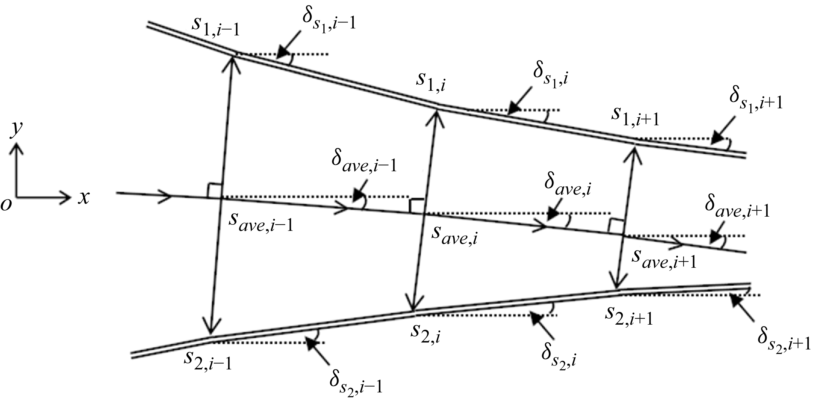
Figure 8 is a schematic illustration of the geometric relationship between the upper and lower sliplines from step
 $i-1$
to step
 $i+1$
during the iterative solution process. During the advancement, this model assumes that the line segment
 $s_{1}s_{2}$
is always perpendicular to the mean flow direction.
Taking the case where
 $s_{2}$
first interacts with the expansion wave as an example, the detailed solution steps are as follows.
-
(i) Given
 $s_{1,i-1}$
and
$s_{2,i-1}$
, and the upper/lower slipline angles
$\delta _{s_1,i-1}$
and
$\delta _{s_2,i-1}$
, compute
$s _{ave,i}$
and the angle
$\delta _{ave,i-1}$
:(3.8)Additionally, at the start of the slipline advancement and solution process,
\begin{align} \left \{ \begin{aligned} &x_{s_{ave}, i}=x_{s_{ave}, i-1}+\mathrm{d}x_{ave},\\[3pt]&y_{s_{ave}, i}=y_{s_{ave}, i-1}+\tan \big(\delta _{ave,i-1}\big)\,\mathrm{dx}_{ave},\\[3pt]&\delta _{ave, i-1}=\frac {1}{2}\big(\delta _{s_1, i-1}+\delta _{s_2, i-1}\big). \end{aligned} \right . \end{align}
$x_{s_{ave},1}={1}/{2}(x_{T_1}+x_{T_2})$
,
$y_{s_{ave},1}={1}/{2}(y_{T_1}+y_{T_2})$
and
$\delta _{ave}={1}/{2}(-\delta _m^{T_{1}}+\delta _m^{T_{2}})$
.
-
(ii) Solve the
$s_{2, i}$
and
$s_{1, i}$
. The equation of the straight
$s_{1,i}s_{2,i}$
is(3.9)and the equations of straight
\begin{align} \begin{aligned} &y-y_{s_{ave}, i}=-\frac {1}{\tan \big(\delta _{ave, i-1}\big)}\big(x-x_{s_{ave}, i}\big)\\ \end{aligned} \end{align}
$s_{1,i-1}s_{1,i}$
,
$s_{2,i-1}s_{2,i}$
are(3.10)By solving (3.9) and (3.10) simultaneously, the coordinates of
\begin{align} \left \{ \begin{aligned} &y-y_{s_{1}, i-1}=-\tan \delta _{s_1,i-1}(x-x_{s_{1}, i-1}),\\[5pt]&y-y_{s_{2}, i-1}=\tan \delta _{s_2,i-1}(x-x_{s_{2}, i-1}).\\ \end{aligned} \right . \end{align}
$s_{2, i}$
and
$s_{1, i}$
can be determined and
$\mathrm{d}x_{s_{2}, i}=x_{s_{2}, i}-x_{s_{2}, i-1}$
,
$\mathrm{d}x_{s_{1}, i}=x_{s_{1}, i}-x_{s_{1}, i-1}$
.
-
(iii) Solve the
$H_{s,i}$
and
$M_{s,i}$
,
$p_{s,i}$
. Here,
$H_{s,i}$
is the height of flow channel and
$H_{s,i}=(y_{s_1,i}-y_{s_2,i})/\cos \delta _{ave,i-1}$
;
$M_{s,i}$
and
$p_{s,i}$
follow the quasi-one-dimensional isentropic flow theory relation(3.11)where
\begin{align} \left \{ \begin{aligned} &\frac {H_{s,i}}{H_{m}}=\frac {M_{m}}{M_{s,i}}\left(\frac {\vartheta \big(M_{s,i}\big)}{\vartheta (M_{m})}\right)^{( {\gamma +1}/{2(\gamma -1))}}, \\&p_{s,i}=p_{m}\left(\frac {\vartheta (M_{m})}{\vartheta \big(M_{s,i}\big)}\right)^{({\gamma }/{\gamma -1})} ,\\ \end{aligned} \right . \end{align}
$M_{m}$
is the average Mach number and can be expressed as the ratio of the average velocity to the average sonic speed (Li & Ben-Dor Reference Li, He, Zhang, Hao, Wu and Liu1997a
,Reference Li, He, Zhang, Hao, Wu and Liu
b
)(3.12)where
\begin{align} \begin{aligned} &M_m=\frac {2\big(\rho _3^{T_1}u_3^{T_1}\cos \delta _m^{T_1}+\rho _Gu_G\big)}{\big(\rho _3^{T_1}+\rho _G \big)\big(a_3^{T_1}+a_G \big)},\\ \end{aligned} \end{align}
$u_3^{T_1}=a_3^{T_1}M_3^{T_1}$
and
$u_G=a_GM_G$
;
$\rho _3^{T_1}$
,
$a_3^{T_1}$
,
$M_3^{T_1}$
are the density, sonic speed and Mach number at region (3) near
$T_1$
;
$\rho _G$
,
$a_G$
$M_G$
can be obtained using the normal shock relations. Here,
$p_{m}$
is the average pressure behind the Mach stem.
-
(iv) Solve
$\delta _{s_1,i}$
and
$\delta _{s_2,i}$
. Based on the pressure equilibrium relation across the slip lines, it follows that
$p_{s_1,i}=p_{s,i}=p_{s_2,i}$
or
$\mathrm{d}p_{s_1,i}=(p_{s,i}-p_{s,i-1})=\mathrm{d}p_{s_2,i}$
. The specific solution methods are as follows: when both
$s_{1}$
and
$s_{2}$
are in the free segment,
$\delta _{s_1,i}$
and
$\delta _{s_2,i}$
can be solved using (3.1) and (3.3); when
$s_{2}$
is in the interference segment and
$s_{1}$
is in the free segment,
$\delta _{s_1,i}$
can be obtained from (3.1),
$\mathrm{d}\delta _{s_2,i-1}$
is derived from (3.5) and
$\delta _{s_2,i}=\delta _{s_2,i-1}+\mathrm{d}\delta _{s_2,i-1}$
; when both
$s_{1}$
and
$s_{2}$
are in the interference segment,
$\mathrm{d}\delta _{s_1,i-1}$
is derived from (3.4) and
$\delta _{s_1,i}=\delta _{s_1,i-1}+\mathrm{d}\delta _{s_1,i-1}$
,
$\mathrm{d}\delta _{s_2,i-1}$
is derived from (3.5) and
$\delta _{s_2,i}=\delta _{s_2,i-1}+\mathrm{d}\delta _{s_2,i-1}$
. -
(v) Solve
$s_{ave, i+1}$
, the average flow angle
$\delta _{ave, i}$
, then repeat steps (i)–(iv) to determine
$s_{1, i+1}$
,
$\delta _{s_1, i+1}$
,
$s_{2, i+1}$
and
$\delta _{s_2, i+1}$
.


3.3. Global solution based on sonic throat compatibility condition
Bai & Wu (Reference Bai and Wu2017) proposed the sonic throat compatibility condition that determines the Mach stem height for classical shock reflection. This condition states that, if the slipline angle is zero
 $\delta _{s}=0$
at the exact location where the sonic throat condition occurs
 $M_{s}=M_{s}^{+}=1$
, then this solution is compatible. Lin et al. (Reference Lin, Bai and Wu2019) subsequently refined this criterion by proposing a throat compatibility condition for asymmetric cases, indicating that the sonic throat (
 $E_{1}E_{2}$
) locates at the position where the angles of the upper and lower slip lines are equal.
As noted in § 2.3, for an asymmetric overexpanded jet, the sonic throats do not coincide with the points of flow horizontalisation. Therefore, in this work, we adopt the throat compatibility condition given by Lin et al. (Reference Lin, Bai and Wu2019):
 \begin{align} \left \{\begin{aligned} &\delta _{s_1}^{E_1} - \delta _{s_2}^{E_2} = 0, \\[3pt] & M_{s_1}^{E_1} = M_{s_2}^{E_2}=1, \\[3pt] &\frac {y_{E_2} - y_{E_1}}{x_{E_2} - x_{E_1}} = -\frac {1}{\tan \delta _{\text{ave}}}, \end{aligned} \right . \end{align}
which means that at the throat location
 $E_{1}$
and
 $E_{2}$
, the Mach number
 $M_{s_1}^{E_1}$
and
 $M_{s_2}^{E_2}$
equal 1, and the flow deflection angles of the two sliplines
 $\delta _{s_1}^{E_1}$
and
 $\delta _{s_2}^{E_2}$
are equal.
Schematic illustration of global solution flowchart.

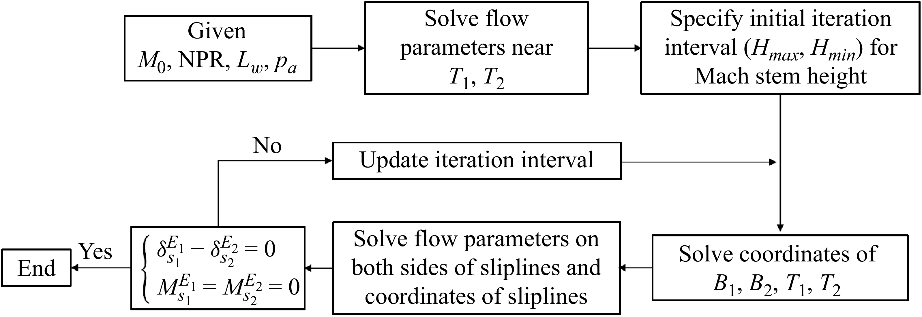
According to the sonic throat compatibility condition for the global model of flow field structures in asymmetric overexpanded jet, the iterative solution flowchart is presented as figure 9, with the specific steps as follows.
-
(i) Solve the flow parameters near the triple points
$T_{1}\,\text{and}\,T_{2}$
, the triple-shock relation can simply estimate the average values of flow parameters. The pressure, Mach number, temperature near the triple points can be solved, and the shock angles and flow deflection angles of the incident shocks, reflected shocks and jet boundaries can also be obtained. -
(ii) According to the nozzle geometry, a solution interval for the Mach stem height is preset as
$(H_{\textit{min}},H_{\textit{max}})$
. At the beginning of the solution process, the upper and lower bounds of the solution interval are preset based on the nozzle geometry, as illustrated in figure 10. The initial value of
$H_{\textit{min}}$
is 0 and the initial value of
$H_{\textit{max}}$
is
$H_{A}(1-L_{w}\tan \beta _{i_1})$
. During the iterative solution process, the Mach stem height solution interval is continuously updated, while the model-predicted Mach stem height remains 0.5 (
$H_{\textit{min}}+H_{\textit{max}}$
). -
(iii) Solve the coordinates of triple points
$T_{1}$
and
$T_{2}$
. Based on the geometric configuration among the incident shock wave, reflected shock wave and Mach stem, the triple point coordinates are determined. Treating the value of
$H_{m}$
obtained from step (ii) as a known quantity, the system yields seven fundamental equations (i.e. (A1)–(A5) in Appendix A) with seven unknowns during the triple point coordinate calculation, thereby admitting a unique solution. -
(iv) Solve the sliplines. The detailed iterative procedure for solving the sliplines has been provided in § 3.2.3. During the solution process, attention should be paid to identifying the positions of
$K_{1}$
and
$K_{2}$
to select the appropriate governing equations. -
(v) Update the Mach stem solution interval using the sonic throat compatibility condition. When computing the Mach stem height
$H_{m}$
in step (ii), the shape of the slipline will be uniquely given whether the solution satisfies the sonic throat compatibility condition or not. However, only solutions that meet the sonic throat compatibility conditions are physical. Therefore, during the solution process, the Mach stem solution interval should be continuously updated based on the following conditions until the throat compatibility condition is met. Additionally, the updated conditions are that if
$\delta _{s_1}^{E_1}-\delta _{s_2}^{E_2}\neq 0,M_{s_1}=M_{s_2}=1$
, then we make
$H_{\textit{min}}=H_{m}$
and if
$\delta _{s_1}^{E_1}-\delta _{s_2}^{E_2}=0,M_{s_1}=M_{s_2}\neq 1$
, then we make
$H_{\textit{max}}=H_{m}$
. In this way, steps (i)–(v) are repeated until the solution to the subsonic region corresponding to the accuracy requirement or the height of Mach stem just meets the sonic throat compatibility condition.


Schematic illustration of initial interval
 $(0,H_{A}(1-L_{w}\tan \beta _{i_1}))$
of Mach stem solution.

4. Theoretical model predictions and analysis
In this section, we analyse the accuracy of the theoretical model in this paper by comparing with previous theoretical models and numerical results under symmetric conditions. By comparing with numerical results, we verified the prediction accuracy of the model under asymmetric conditions. The variation of flow field structure sizes with different nozzle parameters as well as the critical geometric condition for complete misalignment of the interference segment of the upper and lower sliplines is derived.
4.1. Accuracy of the theoretical model for symmetric Mach reflection in an overexpanded jet
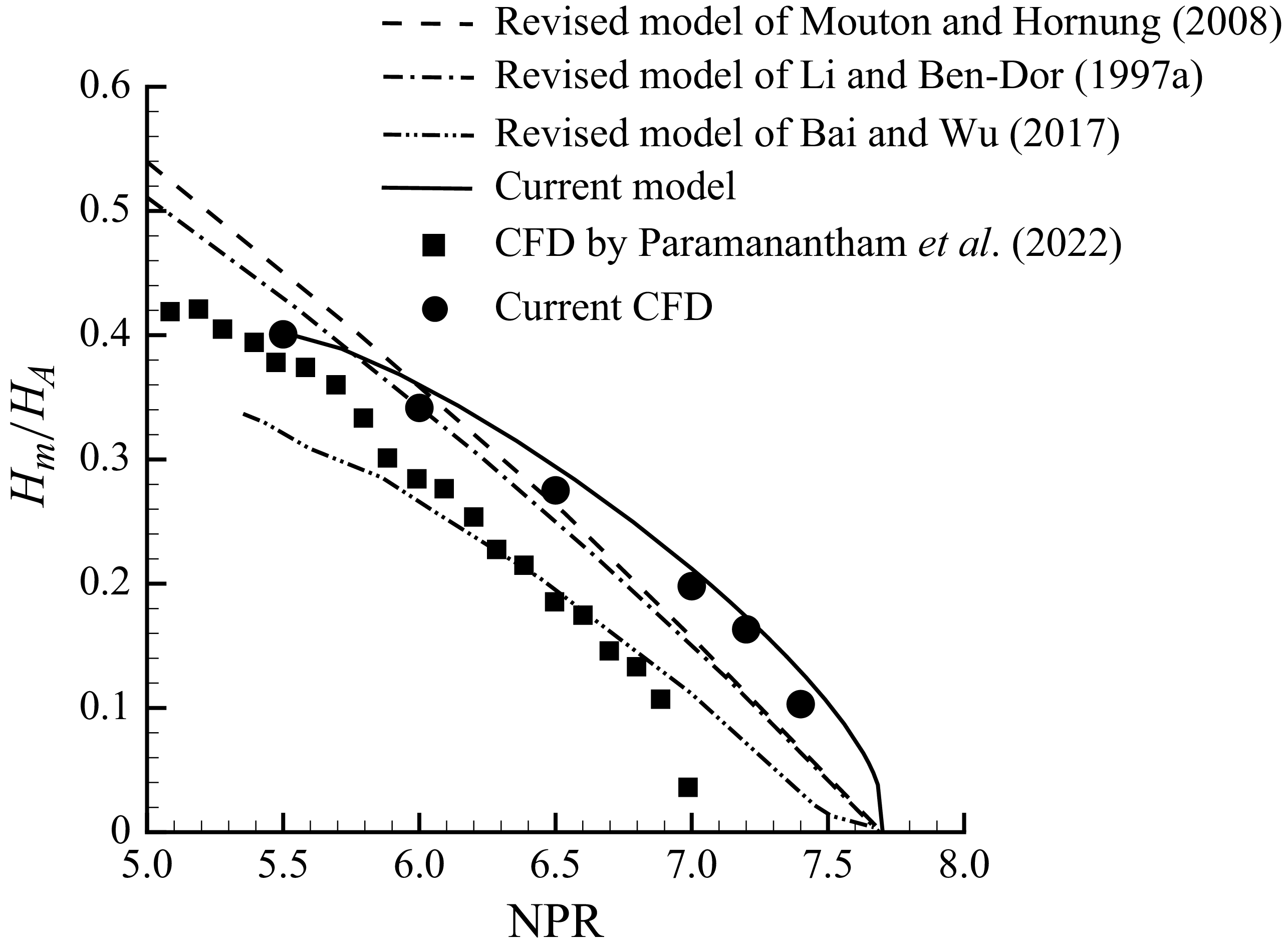
Figure 11 presents Mach stem height predictions of current model and CFD results, comparing model predictions and numerical results proposed by Paramanantham et al. (Reference Paramanantham, Janakiram and Gopalapillai2022) under different NPR conditions at
 $M_{0}=2.75$
. Significant discrepancies exist between the numerical results of this study and those reported by Paramanantham et al. (Reference Paramanantham, Janakiram and Gopalapillai2022). In their study, Paramanantham et al. (Reference Paramanantham, Janakiram and Gopalapillai2022) performed computations for overexpanded jet shock reflection under symmetric conditions using a 400
 $\times$
200 structured grid within a computational domain of
 $4H_{A}\times 2H_{A}$
. Notably, the uniform grid distribution employed proved insufficient for resolving small Mach stems. When the Mach stem height spans a few cells, it becomes easily overlooked. This may explain why their numerical results indicate the disappearance of the Mach stem before reaching the von Neumann point. In contrast, our numerical simulations were conducted on a significantly larger computational domain of
 $10H_{A}\times 15H_{A}$
, while maintaining adequate grid resolution along the Mach stem direction. Particularly for cases with higher NPR values (corresponding to smaller Mach stem height), we ensured a minimum of 150 grid points across the Mach stem height to enhance capture accuracy. This enables our numerical calculations to successfully capture the Mach stem at
 $M_{0}=2.75$
under NPR conditions of 7, 7.2 and 7.4 (prior to reaching the von Neumann point), thereby demonstrating the reliability of our computational approach. Consequently, subsequent comparisons will focus on comparing model predictions with the numerical results from this study. Though all theoretical models accurately predict the NPR corresponding to the von Neumann condition, only our model successfully captures the trend of an increasing slope with NPR and predicts significant Mach stem height even at very low NPR conditions. In general, the Mach stem height predictions from our model demonstrate the best agreement with our numerical results.
Comparison among current CFD results, current theoretical model results and CFD results, and theoretical model results of Paramanantham et al. (Reference Paramanantham, Janakiram and Gopalapillai2022) under
 $M_{0}$
= 2.75.

Comparison of Mach stem height between current model and CFD for symmetric Mach reflection in an overexpanded jet.

Comparison between current model and CFD under
 $M_{0}$
= 3, NPR = 7.

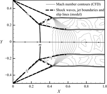
A comparison of the CFD results with the predictions of our model is presented in figure 12 under the conditions of
 $M_{0}=3$
and NPR = 7. The predicted Mach stem height deviation (the relative error of the theoretical model with respect to the CFD results) is 3.70
 $\%$
. Mach number contours obtained by CFD are shown with the solid lines, while the dashed lines depict the model predictions. The predicted triple points and reflected shock waves exhibit a slight upstream shift compared with the CFD results. In general, the incident/reflected shock waves, jet boundaries and sliplines predicted by the current model show good agreement with the CFD results.
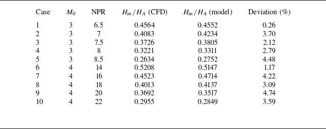
Table 3 presents further results of the Mach stem height obtained from the theoretical model and CFD, along with the corresponding deviations, under various nozzle exit conditions. The model-predicted Mach stem height is slightly larger than the CFD results. Maximum deviation of the model-predicted Mach stem height is 4.48 % for
 $M_{0}$
= 3. Maximum deviation of the model-predicted Mach stem height is 4.74 % for
 $M_{0}$
= 4. In general, the model demonstrates high accuracy in predicting the Mach stem height for symmetric shock reflection.
Influence analysis of individual nozzle exit parameters. (a) Influence of NPR on Mach stem height under different
 $M_{0}$
. (b) Influence of
 $M_{0}$
on Mach stem height under different NPR.

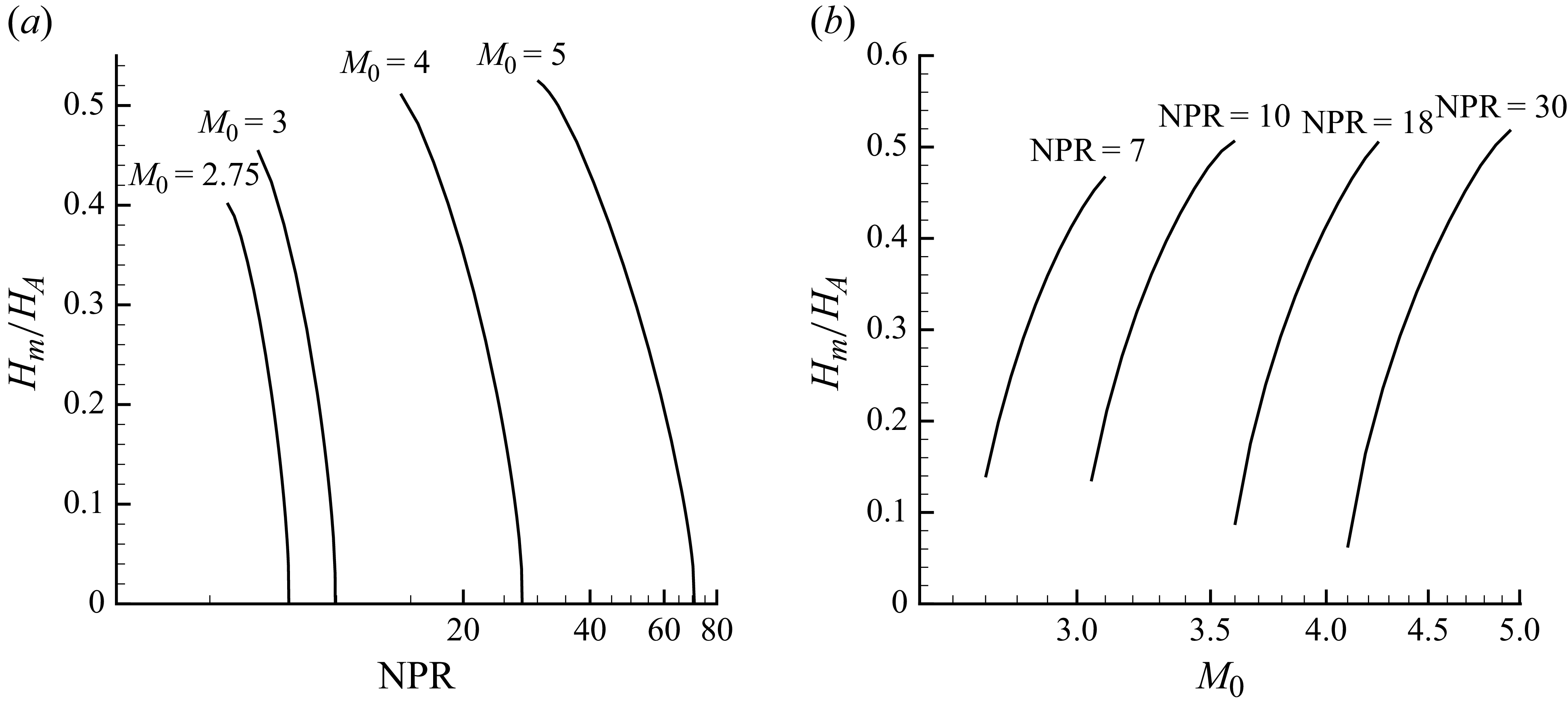
Additionally, figure 13 provides further results on the influence of the Mach stem height with nozzle exit parameters as predicted by the model. Figure 13(a) shows the influence of Mach stem height with NPR under different
 $M_{0}$
conditions. The Mach stem height decreases as NPR increases and the rate of decrease accelerates with larger NPR. Furthermore, in logarithmic coordinates, as
 $M_{0}$
increases, the curve between NPR and Mach stem height becomes increasingly flat. Figure 13(b) shows the influence of Mach stem height with
 $M_{0}$
under different NPR conditions. The Mach stem height increases as
 $M_{0}$
increases and the rate of increase decelerates with larger NPR. Furthermore, under different NPR conditions, the curves between
 $M_{0}$
and Mach stem height are approximately parallel.
In summary, the numerical method employed in this paper provides more accurate capture of flow field structures in symmetric jet Mach reflection. Additionally, our model demonstrates an excellent predictive capability for the flow field structure. The maximum deviation between model-predicted Mach stem height and numerical results does not exceed 4.74 % for both the
 $M_{0}=3$
and
 $M_{0}=4$
cases. Additionally, the Mach stem height decreases as NPR increases and
 $M_{0}$
decreases.
4.2. Accuracy of the theoretical model for asymmetric Mach reflection in an overexpanded jet
Figure 14 presents a comparison between the current model and CFD under
 $M_{0}$
= 2.75, NPR = 6 and
 $L_{w}$
= 0.1. The streamline passing through y = 0 is depicted. Due to the geometric asymmetry of the nozzle (
 $L_w$
= 0.1), the flow is deflected downward, resulting in streamline deviation towards the lower region. The predicted Mach stem height deviation is 2.76
 $\%$
. The Mach number contour obtained by CFD is shown with the solid lines, while the dashed lines depict the model predictions. The predicted triple points exhibit good agreement compared with the CFD results. In general, the incident/reflected shock waves, jet boundaries and sliplines predicted by the model show good agreement with the CFD results.
Comparison between current model and CFD under
 $M_{0}$
= 2.75, NPR = 6 and
 $L_{W}$
= 0.1.

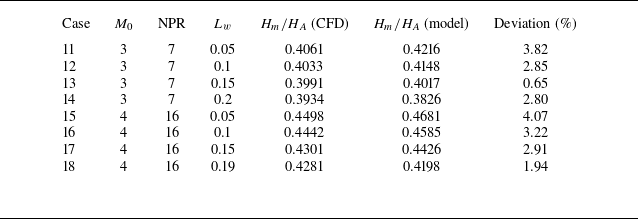
Table 4 presents the height of the Mach stem obtained by the current model, CFD and deviations under different nozzle exit conditions. The model-predicted Mach stem height remains slightly larger than the CFD results. Compared with the prediction accuracy for symmetric Mach reflection, the model’s accuracy for asymmetric Mach reflection shows a slight decrease. Maximum deviation of the model-predicted Mach stem height does not exceed 3.82 % for
 $M_{0}=3$
and NPR = 7. The maximum deviation of the model-predicted Mach stem height does not exceed 4.07 % for
 $M_{0}=4$
and NPR = 16. In general, the model demonstrates high accuracy in predicting the Mach stem height for asymmetric jet flow. Additionally, both CFD and current model results consistently demonstrate that the Mach stem height decreases as
 $L_{w}$
increases.
Comparison of Mach stem height between current model results and CFD results for an asymmetric jet.

When the
 $M_{0}$
and
 $\mathrm{NPR}$
are given, the triangles
 $A_{1}B_{1}T_{1}$
and
 $A_{2}B_{2}T_{2}$
(figure 7) formed by the incident shocks, reflected shocks and jet boundaries above and below are similar. Changing the unilateral
 $L_{W}$
actually alters the geometric size of the corresponding triangle. When
 $L_{W}$
increases, the lower triangle
 $A_{2}B_{2}T_{2}$
continuously decreases in size. This change is transmitted to the slipline via expansion waves, altering the geometric shape of the boundary of the subsonic region downstream of the Mach stem (i.e. the slipline). With the nozzle exit flow parameters remaining unchanged, the shock angle does not change; instead, the Mach stem moves in the downstream direction, ultimately resulting in a reduction in its height.
4.3. Influence of nozzle exit conditions on Mach stem height
For asymmetric Mach reflection in an overexpanded jet, there is an additional parameter
 $L_w$
that affects the Mach stem height comparing with the symmetric Mach reflection. Referring to the theoretical formula for the parameters influencing the Mach stem height for symmetric Mach reflection (Paramanantham et al. Reference Paramanantham, Janakiram and Gopalapillai2022), we can provide the theoretical formula for asymmetric Mach reflection as
 \begin{align} \begin{aligned} \frac {H_{m}}{H_{A}}=f(M_{0}, \mathrm{NPR},L_{w}, \gamma ). \end{aligned} \end{align}
Influence analysis of individual nozzle exit parameters. (a) Influence of NPR on Mach stem height with increasing
 $L_{w}$
under
 $M_{0}=3$
. (b) Influence of
 $M_{0}$
on Mach stem height with increasing
 $L_{w}$
under NPR = 7.

Influence analysis of individual nozzle exit parameters. (a) Influence of NPR on the effect of
 $L_w$
reduction on Mach stem height under
 $M_{0}=3$
. (b) Influence of NPR on Mach stem height with different
 $M_{0}$
under
 $L_{w}=0.1$
.

Influence analysis of individual nozzle exit parameters. (a) Influence of
 $M_{0}$
on the effect of
 $L_w$
reduction on Mach stem height under NPR = 7. (b) Influence of
 $M_{0}$
on Mach stem height with different NPR under
 $L_{w}=0.1$
.

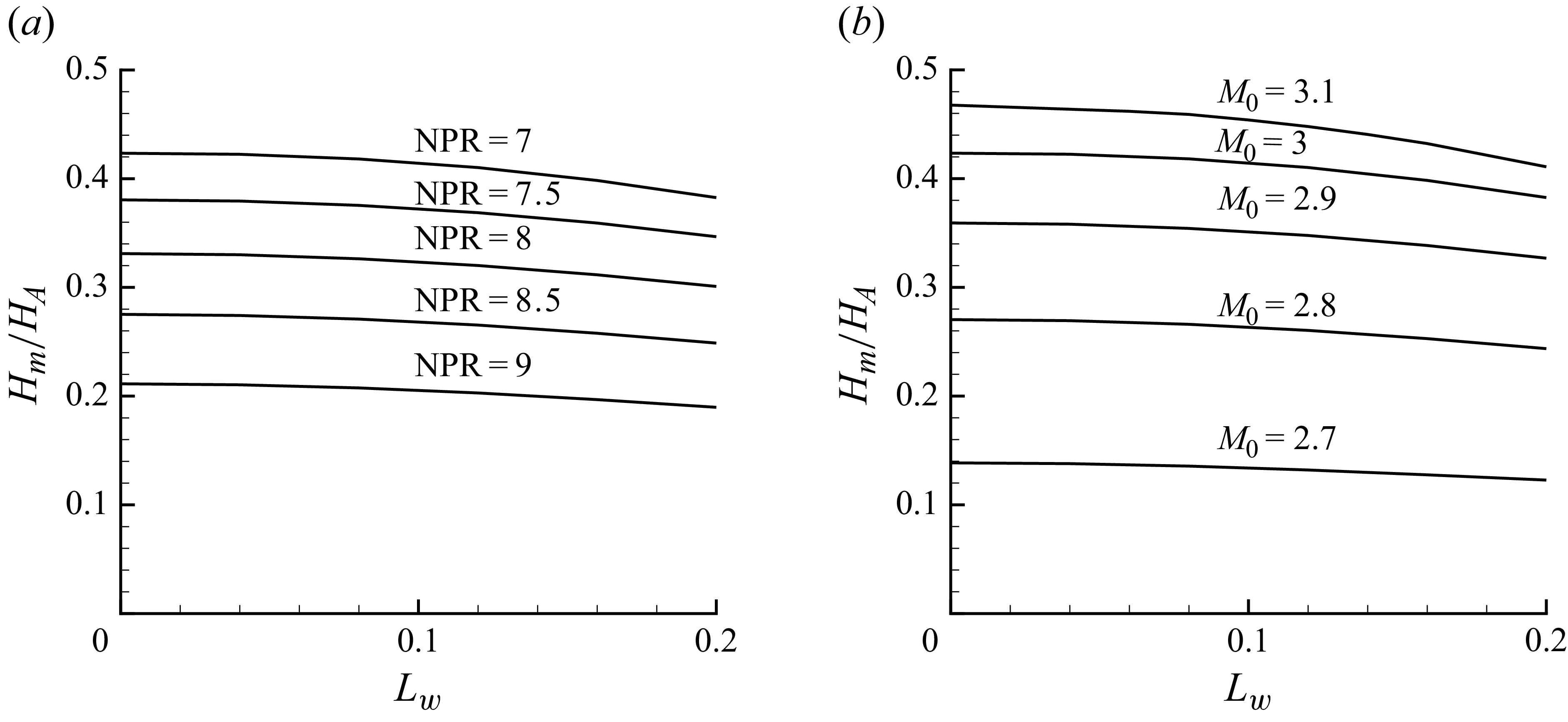
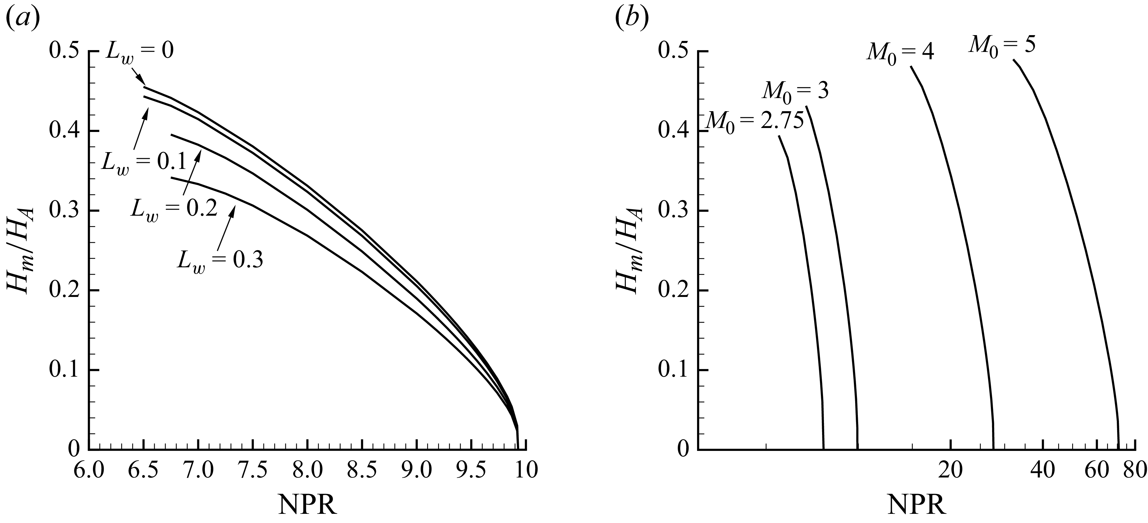
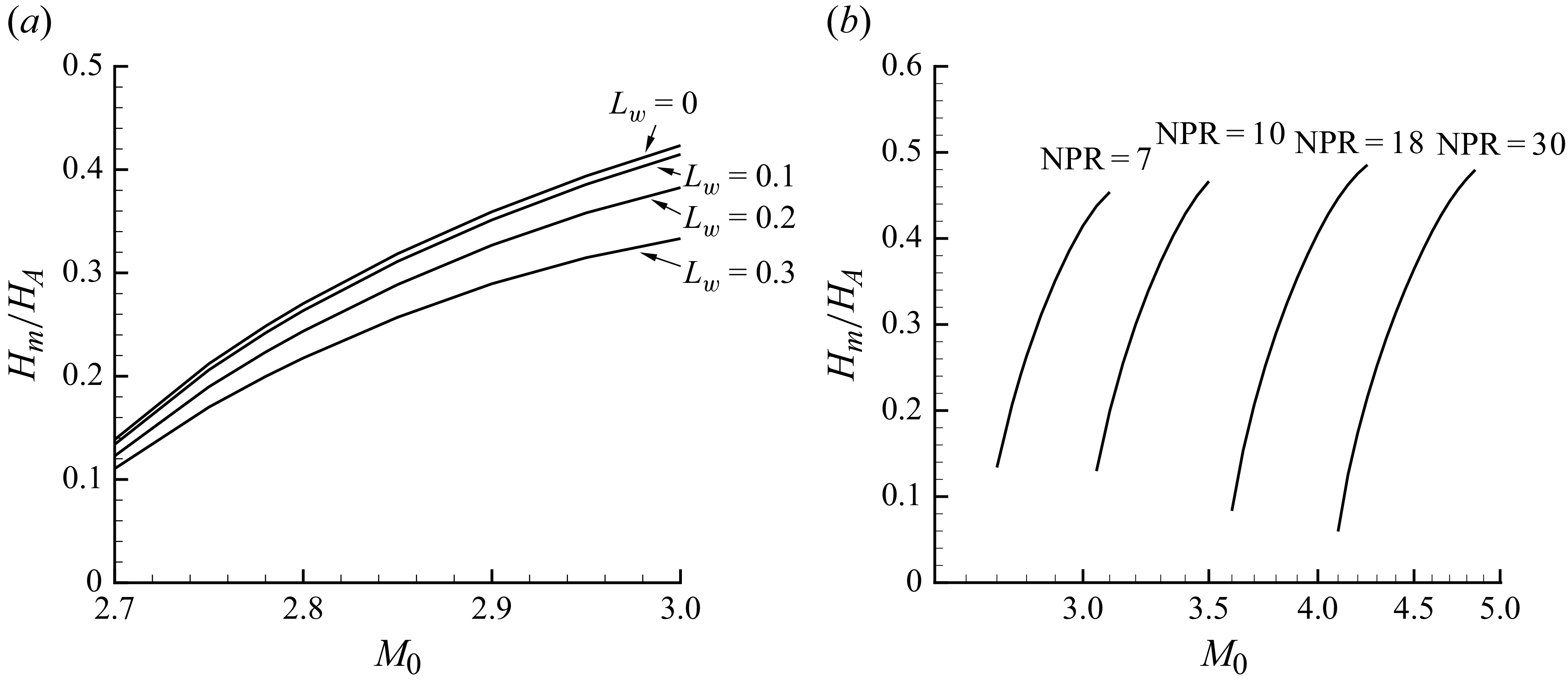
Next, we will analyse the effects of several parameters on the Mach stem height. The model-predicted results under different nozzle exit conditions are presented in figures 15, 16 and 17.
Figure 15(a) presents the variation of Mach stem height with
 $L_{w}$
under different NPR and
 $M_{0}=3$
. Mach stem height slightly decreases as
 $L_{W}$
increases. The model predicts that the Mach stem height at
 $L_w = 0.2$
is 9.64 % lower than that at
 $L_w = 0$
for NPR = 7. In comparison, the model predicts that the Mach stem height at
 $L_w = 0.2$
is 10.23 % lower than that at
 $L_w = 0$
for NPR = 9. This indicates that an increase in NPR enhances the reducing effect of
 $L_{w}$
on the Mach stem height.
Figure 15(b) presents the variation of Mach stem height with
 $L_{w}$
under different
 $M_{0}$
and NPR = 7. The model predicts that the Mach stem height at
 $L_w = 0.2$
is 12.14 % lower than that at
 $L_w = 0$
for
 $M_{0}$
= 3.1. In comparison, the model predicts that the Mach stem height at
 $L_w = 0.2$
is 11.42 % lower than that at
 $L_w = 0$
for
 $M_{0}$
= 2.7. This indicates that an increase in
 $M_{0}$
enhances the reducing effect of
 $L_{w}$
on the Mach stem height.
Figure 16(a) presents the variation of Mach stem height with NPR under different
 $L_{w}$
and
 $M_{0}=3$
. The Mach stem height decreases as NPR increases. The model predicts that the Mach stem height at NPR = 9 is 50.08 % lower than that at NPR = 7 for
 $L_w = 0$
. In comparison, the model predicts that the Mach stem height at NPR = 9 is 48.69 % lower than that at NPR = 7 for
 $L_w = 0.3$
. This indicates that an increase in
 $L_{w}$
weakens the reducing effect of NPR on the Mach stem height.
Figure 16(b) presents the variation of Mach stem height with NPR under different
 $M_{0}$
and
 $L_{w}=0.1$
. When compared with the results of the symmetric case (
 $L_{w}=0$
) in figure 13(a), the curve forms remain largely consistent. Only a slight decrease in Mach stem height is observed, ultimately decreasing to zero at the NPR corresponding to the von Neumann condition.
Figure 17(a) presents the variation of Mach stem height with
 $M_{0}$
under different
 $L_{w}$
and NPR = 7. The Mach stem height increases as
 $M_{0}$
increases. The model predicts that the Mach stem height at
 $M_{0}=3$
is 205.55 % higher than that at
 $M_{0}=2.7$
for
 $L_w = 0$
. In comparison, the model predicts that the Mach stem height at
 $M_{0}=3$
is 201.80 % higher than that at
 $M_{0}=2.7$
for
 $L_w = 0.3$
. This indicates that an increase in
 $L_{w}$
weakens the enhancement effect of
 $M_{0}$
on the Mach stem height.
Figure 17(b) presents the variation of Mach stem height with
 $M_{0}$
under different NPR and
 $L_{w}=0.1$
. Similarly, when compared with the symmetric case (
 $L_{w}=0$
) results in figure 13(b), the curve forms remain largely consistent. Only a slight decrease in Mach stem height is observed and the Mach stem height increases with the Mach number.
In summary, an increase in
 $L_w$
weakens both the reducing effect of NPR and the enhancement effect of
 $M_{0}$
on the Mach stem height. Furthermore, the reducing effect of
 $L_{w}$
is slightly enhanced by the increase in NPR and the increase in
 $M_{0}$
.
4.4. Critical geometric condition for complete misalignment of the interference segment of the upper and lower sliplines
As
 $L_{w}$
gradually increases, the flow field structure will evolve from figure 14 into the form shown in figure 18(a), which presents the Mach number contour under
 $L_{w}$
= 0.3,
 $M_{0}$
= 4 and NPR = 18. It can be observed that the interference segment of upper and lower sliplines become completely misaligned, which means the last expansion wave from one side interacts with the slipline, while the first expansion wave from the opposite side does not interact with the slipline. The Mach number contour line of 1 is marked and the sonic throat location shifts.
A critical flow field structure can be defined, schematically illustrated in figure 18(b). This critical state occurs when the last expansion wave generated by the reflected shock on one side (
 $B_2F_2$
in figure 18
b) precisely impinges on the slipline, while the first expansion wave from the opposite reflected shock (
 $B_1K_1$
in figure 18
b) just begins to interact with the slipline. The theoretical model used in this study can be employed to predict
 $L_{w}$
for this condition, which is termed
 $L_{w}^{\textit{crit}}$
.
(a) Mach number contours (grey solid lines) and characteristic lines (black solid lines) under
 $M_{0}$
= 4, NPR = 18,
 $L_{w}=0.3$
. (b) Schematic illustration of the flow field structures of the complete misalignment of the interference segment of upper/lower sliplines.

Influence of NPR on
 $L_{w}^{\textit{crit}}$
at different
 $M_{0}$
.

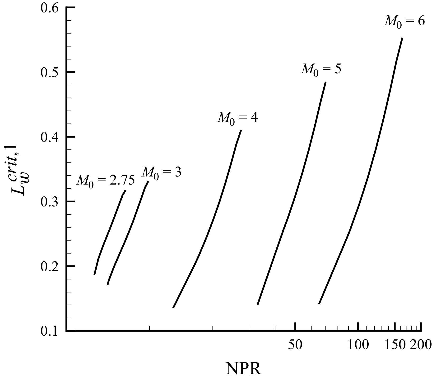
Figure 19 is the prediction of corresponding
 $L_{w}^{\textit{crit}}$
at different NPR when given
 $M_{0}$
. For lower nozzle exit Mach numbers (
 $M_{0}$
= 2.75 and
 $M_{0}$
= 3), the curves show a slight upward convexity. Before the inflection point,
 $L_{w}^{\textit{crit}}$
increases rapidly with NPR; after the inflection point, the growth rate slows down, which indicates that the enhancement effect of the NPR on
 $L_{w}^{\textit{crit}}$
gradually weakens under low-Mach-number conditions. In contrast, for higher Mach numbers (
 $M_{0}$
= 4, 5, 6), the curves show a slight concavity downward. Before the inflection point,
 $L_{w}^{\textit{crit}}$
increases slowly with NPR; after the inflection point, the growth rate accelerates, which indicates that the enhancement effect of the NPR on
 $L_{w}^{\textit{crit}}$
gradually intensifies under high-Mach-number conditions. For a given NPR,
 $L_{w}^{\textit{crit}}$
decreases as
 $M_0$
increases. At
 $ \textit{NPR}=6.5$
,
 $L_{w}^{\textit{crit}}$
is 0.26 for
 $M_0=2.75$
and 0.18 for
 $M_0=3$
, representing a decrease of 30.77 % when
 $M_0$
increases from 2.75 to 3. For a given Mach number,
 $L_{w}^{\textit{crit}}$
increases with increasing NPR. At
 $M_0=4$
,
 $L_{w}^{\textit{crit}}$
is 0.14 for
 $\mathrm{NPR}=13$
and 0.41 for
 $\mathrm{NPR}=27.5$
, representing an increase of 192.86 % when NPR increases from 13 to 27.5.
The trend of how
 $L_{w}^{\textit{crit}}$
changes with NPR and
 $M_{0}$
can be easily understood by considering the degree of overexpansion. When other conditions remain constant, decreasing the Mach number or increasing the NPR both lead to a reduction in the intensity of the incident shock wave. In conditions of lower overexpansion (i.e. at lower NPR), the weakened incident shock wave intensity signifies a decrease in the shock wave angle. When the shock wave angle of the incident shock wave decreases, it geometrically results in an increase in the streamwise length of the interaction segments (interference segments) between expansion waves and sliplines. However, increasing
 $L_{w}$
actually reduces the length of the lower interference segment and shifts it upstream. When the upper interference segment lengthens, the lower interference segment has more space to move upstream, thereby achieving a larger
 $L_{w}^{\textit{crit}}$
.
5. Concluding remarks
This study focuses on asymmetric shock reflection in a supersonic overexpanded jet induced by nozzle geometric asymmetry, and systematically conducts research through numerical simulations and a theoretical model. The key conclusions are as follows.
-
(i) Through CFD simulations, we confirm that the flow field structures are highly sensitive to the computational domain and grid density along the Mach stem. Based on independence tests, the computational domain (
$10H_A\times 15H_A$
) and grid configuration (
$\geqslant$
150 nodes along the Mach stem) are determined, providing a stable foundation for subsequent theoretical model verification. -
(ii) A theoretical model is established and can predict the size and shape of flow field structures (shocks, expansion waves, sliplines). For symmetric shock reflection, the maximum deviation of Mach stem height predicted by the theoretical model is 4.74 % compared with CFD results. For asymmetric shock reflection, the maximum deviation of the Mach stem height predicted by the theoretical model is 4.07 %, demonstrating good consistency with CFD results.
-
(iii) Influence of nozzle exit conditions on the Mach stem height is studied: the Mach stem height decreases with the increase of NPR and
$L_w$
, and decreases as the nozzle exit Mach number (
$M_0$
) decreases. Additionally, an increase in
$L_w$
weakens both the reducing effect of NPR and the enhancement effect of
$M_{0}$
on the Mach stem height. The reducing effect of
$L_{w}$
is enhanced by the increase in NPR and the increase in
$M_{0}$
. -
(iv) The critical nozzle exit length difference (
$L_w^{\textit{crit}}$
), corresponding to the complete misalignment of the interference segment of upper and lower sliplines, is given. This critical value increases with increasing NPR and decreases with increasing
$M_0$
.


This study enriches the theoretical study of asymmetric shock reflection in an overexpanded jet, and the proposed model and obtained laws offer important support for the design of supersonic aircraft engines.
Acknowledgements
The authors are grateful to all referees for their useful comments and references, which helped improve the manuscript.
Funding
The authors appreciate the financial support from Tianmushan Laboratory (Grant No. TK-2024-D-004), the National Natural Science Foundation of China (Nos. 12472232 and 52192632), and the Beihang University Young Elite Talent Support Program (No. 501XYGG2025105003).
Declaration of interests
The authors report no conflict of interest.
Appendix A. Geometric relations and three shock-wave theory for solving triple points
Here, we will discuss the geometric relationships that will be used to solve the incident shock waves, reflected shock waves, jet boundaries and Mach stem when the Mach stem height
 $H_{m}$
is determined. Figure 20 is a schematic illustration of geometric relationships among the incident shock waves, reflected shock waves, jet boundaries and Mach stem. Here,
 $H_{A}$
represents the nozzle diameter and we have the coordinates of
 $A_{1}$
and
 $A_{2}$
.
 \begin{align} \left \{\begin{aligned} &x_{A_{1}}=0,\\[3pt]&x_{A_{2}}=L_{w},\\[3pt]&y_{A_{1,2}}=\pm \frac {1}{2}H_{A}, \end{aligned} \right . \end{align}
where the definition of
 $L_{w}$
is provided in § 2.1. By taking flow structures located in the upper half of the x-axis as an example, the equations for the incident shock
 $A_1T_1$
can be confirmed:
 \begin{align} \begin{aligned} &y-y_{A_1}=-\tan \big(\beta _{i_1}\big)\big(x-x_{A_1}\big)\\ \end{aligned} \end{align}
and the jet boundary
 $A_1B_1$
is
 \begin{align} \begin{aligned} &y-y_{A_1}=-\tan \big(\delta _{i_1}\big)\big(x-x_{A_1}\big),\\ \end{aligned} \end{align}
where
 $\beta _{i_1}$
is the shock angle of upper incident shock and
 $\delta _{i_1}$
is equal to the flow deflection angle of the upper incident shock. The solution of incident shock
 $i_{2}$
and jet boundary
 $A_{2}T_{2}$
follow the same rule.
Schematic illustration of geometric relationships among the incident shock waves, reflected shock waves, jet boundaries and Mach stem. Here,
 $i_{1}$
and
 $i_{2}$
represent incident shock waves;
 $r_{1}$
and
 $r_{2}$
represent reflected shock waves.

Then, Lin et al. (Reference Lin, Bai and Wu2019) used the circular arc assumption for the Mach stem, and successfully solved the flow structures for classical asymmetric shock reflection problems. Here, the same assumption is adopted to solve the coordinate of the triple points. As shown in figure 7, the triple points,
 $T_{1}$
,
 $T_{2}$
, lie on the Mach stem and incident shock waves (
 $i_{1}$
and
 $i_{2}$
), which means that the following geometrical relations hold:
 \begin{align} \left \{ \begin{aligned} &y_{T_{1}}-y_{A_{1}}=-\tan \big(\beta _{i_1}\big)\big(x_{T_{1}}-x_{A_{1}}\big), \\[3pt]&y_{T_{2}}-y_{A_{2}}=\tan \big(\beta _{i_2}\big)\big(x_{T_{2}}-x_{A_{2}}\big) ,\\[3pt]&\big(x_{T_{1}}-x_{O}\big)^{2}+\big(y_{T_{1}}-y_{O}\big)^{2}=R^{2},\\[3pt]&\big(x_{T_{2}}-x_{O}\big)^{2}+\big(y_{T_{2}}-y_{O}\big)^{2}=R^{2}, \end{aligned} \right . \end{align}
where
 $\beta _{i_2}$
is the shock angle of lower incident shock, O is the centre of the circle where the Mach stem is located and R is the radius of the circle. The assumption also gives the tangential relations between incident shock (
 $i_{1}$
and
 $i_{2}$
) and Mach stem (
 $T_{1}T_{2}$
). The slopes of Mach stem at the triple points can be obtained by using the circular shape relation. Additionally, these slopes are equal to the tangent of shock angles
 $\beta _{m}^{T_1}$
and
 $\beta _{m}^{T_2}$
. By giving the Mach stem length
 $H_{m}$
in advance, we have
 \begin{align} \left \{ \begin{aligned} & \big(x_{T_{1}}-x_{T_{2}}\big)^{2}+ \big(y_{T_{1}}-y_{T_{2}}\big)^{2}=H_{m}^{2},\\[3pt]&\frac {y_{T_1}-y_{O}}{x_{T_1}-x_{O}}=\frac {1}{\tan \big(\beta _{m}^{T_1}\big)},\\[3pt]&\frac {y_{T_2}-y_{O}}{x_{T_2}-x_{O}}=-\frac {1}{\tan \big(\beta _{m}^{T_2}\big)}. \end{aligned} \right . \end{align}
The tangent of shock angles
 $\beta _{i_1}$
,
 $\beta _{i_2}$
,
 $\beta _{m}^{T_1}$
and
 $\beta _{m}^{T_2}$
, and the flow deflection angle
 $\delta _{i_1}$
can be obtained by using the classical oblique shock wave relations and the three-shock theory (von Neumann Reference von Neumann1945).
There are seven unknown parameters, and seven equations in (A4) and (A5), so we can uniquely solve the unknowns
 $x_{T_{1}},x_{T_{2}},y_{T_{1}},y_{T_{2}},x_{O},y_{O},R$
. Then, the equation for the straight line of the reflected shock can be established. Here, the upper reflected shock is again taken as an example:
 \begin{align} \begin{aligned} &y-y_{T_1}=\tan \big(\beta _{r_1}-\delta _{i_1}\big)\big(x-x_{T_1}\big),\\ \end{aligned} \end{align}
where
 $\beta _{r_1}$
is the shock angle of upper reflected shock. By solving (A2) and (A6) simultaneously, the coordinates of points
 $B_{1}$
can be determined. The solution of
 $B_{2}$
follows the same rule.
Appendix B. Solution for the interference segments of sliplines
Here, we take the lower slipline
 $s_{2}$
interference segment as an example to derive the governing equations of flow parameters. For the expansion waves in region (7), their geometric morphology satisfies the following differential form of the curve equation:
 \begin{align} \begin{aligned} \mathrm{d}y_{s_2} - \tan \varLambda _2\, \mathrm{d}x_{s_2} &= \big(x_{s_2} - x_{B_2}\big) \big(\varLambda _{\theta _{12}}\, \mathrm{d}\theta _{12} + \varLambda _{\theta _{22}}\, \mathrm{d}\theta _{22}\big) \cos ^{-2} \varLambda _2, \end{aligned} \end{align}
where the
 $\mathrm{d}y_{s_2}$
and
 $\mathrm{d}x_{s_2}$
are the coordinate increments along the slipline
 $s_{2}$
and
 $\mathrm{d}y_{s_2}=\tan \delta _{s_2}\mathrm{d}x_{s_2}$
;
 $x_{B_2}$
is the x-coordinate of
 $B_{2}$
;
 $\theta _{12}=\theta _{B_2}+\mu _{B_2}$
,
 $\theta _{22}=\theta _{s_2}+\mu _{s_2}$
are the angles between the expansion wave and the x-axis at
 $B_{2}$
and near the slipline
 $s_2$
, respectively. Additionally, we have
 \begin{align} \left \{ \begin{aligned} &\varLambda _2(\theta _{12},\theta _{22})=\arctan \frac {2\tan \theta _{12}+\tan (\theta _{22}-\theta _{12})}{2-\tan \theta _{12}\tan (\theta _{22}-\theta _{12})},\\[3pt] &\varLambda _{\theta _{12}}(\theta _{12},\theta _{22})=-\frac {\tan ^2(\theta _{12}-\theta _{22})-2}{\tan ^2(\theta _{12}-\theta _{22})+4},\\[3pt] &\varLambda _{\theta _{22}}(\theta _{12},\theta _{22})=\frac {2\tan ^2(\theta _{12}-\theta _{22})+2}{\tan ^2(\theta _{12}-\theta _{22})+4}.\\ \end{aligned} \right . \end{align}
By taking the differentials of
 $\theta _{12}$
and
 $\theta _{22}$
, we can have
 $ \mathrm{d}\theta _{12}=\mathrm{d}\theta _{B_2}+\mathrm{d}\mu _{B_2}=(1+({\mathrm{d}\mu _{B_2}}/{\mathrm{d}\theta _{B_2}}))\,\mathrm{d}\theta _{B_2}$
and
 $ \mathrm{d}\theta _{22}=\mathrm{d}\theta _{s_2}+\mathrm{d}\mu _{s_2}$
. For
 $ \mathrm{d}\theta _{12}$
, we introduce the relationship between the Mach angle and the flow deflection angle under a small deflection increment
 $\mathrm{d}\theta _{B_2}$
within the expansion wave. For
 $ \mathrm{d}\theta _{22}$
, we further incorporate the relationship between the Mach angle and the Mach number, along with the compatibility condition valid along the streamline (characteristic line
 $C_0$
). Ultimately, the following expression is obtained:
 \begin{align} \left \{ \begin{aligned} &\mathrm{d}\theta _{12}= \big(1+\varPsi _{\mu }\big(M_{B_2}\big)\big)\,\mathrm{d}\theta _{B_2},\\[6pt]&\mathrm{d}\theta _{22}=\mathrm{d}\delta _{s_2}+\frac {\varOmega _{M}\big(M_{s_2}\big)\varPsi _{M}\big(M_{s_2}\big)}{\varPsi _{p}\big(M_{s_2}\big)}\frac {\mathrm{d}p_{s_2}}{p_{s_2}},\\ \end{aligned} \right . \end{align}
where
 \begin{align} \left \{ \begin{aligned} &\varPsi _{\mu }(M)=\frac {\vartheta (M)}{M^2-1},\\[3pt]&\varOmega _{M}(M)=-\frac {1}{M\sqrt {M^{2}-1}},\\[3pt]&\varPsi _{M}(M)=-\frac {M\vartheta (M)}{\sqrt {M^{2}-1}}.\\ \end{aligned} \right . \end{align}
Subsequently, we supplement the differential form of the compatibility relation valid along the characteristic line (
 $C_{-}$
),
 \begin{align} \left \{ \begin{aligned} &\mathrm{d}\theta _{B_2}-\mathrm{d}\delta _{s_2}=\varPhi _{B_2s_2}\big(\mathrm{d}p_{s_2}-\mathrm{d}p_{B_2}\big),\\[3pt]&\varPhi _{B_2s_2}=\frac {1}{2} \big(\varPhi _{B_2}+\varPhi _{s_2}\big),\varPhi (p,M)=\frac {\sqrt {M^{2}-1}}{\gamma M^{2}p}.\\ \end{aligned} \right . \end{align}
By supplementing the relationship between pressure and flow deflection angle under a small deflection increment, we get
 \begin{align} \begin{aligned} \mathrm{d}p_{B_2}=p_{B_2}\varPsi _{p}\big(M_{B_2}\big)\,\mathrm{d}\theta _{B_2}. \end{aligned} \end{align}
Finally, substituting (B2) into (B1) and combining with (B5), we obtain expressions for solving
 $\mathrm{d}\theta _{B_2}$
and
 $\mathrm{d}\delta _{s_2}$
,
 \begin{align} \left \{ \begin{aligned} &\mathrm{d}\theta _{B_2}=\frac {L_{22}\varPhi _{B_2s_2}\,\mathrm{d}p_{s_2}+L_{32}}{L_{12}+L_{22}\big(1+\varPhi _{B_2s_2}p_{B_2}\varPsi _{p}\big(M_{B_2}\big)\big)},\\[4pt]&\mathrm{d}\delta _{s_2}=\big(1+\varPhi _{B_2s_2}p_{B_2}\varPsi _{p}\big(M_{B_2}\big)\big)\,\mathrm{d}\theta _{B_2}-\varPhi _{B_2s_2}\,\mathrm{d}p_{s_2},\\[4pt]&L_{12}=\big(x_{s_2} - x_{B_2}\big)\varLambda _{\theta _{12}}\cos ^{-2} \varLambda _2\big(1+\varPsi _{\mu }\big(M_{B_2}\big)\big),\\[4pt]&L_{22}=\big(x_{s_2} - x_{B_2}\big)\varLambda _{\theta _{22}}\cos ^{-2} \varLambda _2,\\[4pt]&L_{32}=\big(\tan \delta _{s_2}-\tan \varLambda _2\big)\,\mathrm{d}x_{s_2}-\big(x_{s_2} - x_{B_2}\big)\varLambda _{\theta _{22}}\cos ^{-2} \varLambda _2\frac {\varOmega _{M}\big(M_{s_2}\big)\varPsi _{M}\big(M_{s_2}\big)}{\varPsi _{p}\big(M_{s_2}\big)}\frac {\mathrm{d}p_{s_2}}{p_{s_2}} .\end{aligned} \right . \end{align}
The process of solving for
 $\mathrm{d}\theta _{B_1}$
and
 $\mathrm{d}\delta _{s_1}$
is similar, and only the final results are presented here:
 \begin{align} \left \{ \begin{aligned} &\mathrm{d}\theta _{B_1}=\frac {L_{21}\varPhi _{B_1s_1}\mathrm{d}p_{s_1}+L_{31}}{L_{11}+L_{21} \big(1+\varPhi _{B_1s_1}p_{B_1}\varPsi _{p}\big(M_{B_1}\big)\big)},\\[4pt]&\mathrm{d}\delta _{s_1}= \big(1+\varPhi _{B_1s_1}p_{B_1}\varPsi _{p}\big(M_{B_1}\big)\big)\mathrm{d}\theta _{B_1}-\varPhi _{B_1s_1}\,\mathrm{d}p_{s_1},\\[4pt]&L_{11}=-\big(x_{s_1} - x_{B_1}\big)\varLambda _{\theta _{11}}\cos ^{-2} \varLambda _1\big(1+\varPsi _{\mu }\big(M_{B_1}\big)\big),\\[4pt]&L_{21}=-\big(x_{s_1} - x_{B_1}\big)\varLambda _{\theta _{21}}\cos ^{-2} \varLambda _1,\\[4pt]&L_{31}=\big(-\tan \delta _{s_1}-\tan \varLambda _1\big)\,\mathrm{d}x_{s_1}+\big(x_{s_1} - x_{B_1}\big)\varLambda _{\theta _{21}}\cos ^{-2} \varLambda _1\frac {\varOmega _{M}\big(M_{s_1}\big)\varPsi _{M}\big(M_{s_1}\big)}{\varPsi _{p}\big(M_{s_1}\big)}\frac {\mathrm{d}p_{s_1}}{p_{s_1}} ,\end{aligned} \right . \end{align}
where
 $\mathrm{d}y_{s_1}$
and
 $\mathrm{d}x_{s_1}$
are the coordinate increments along the slipline
 $s_{1}$
and
 $\mathrm{d}y_{s_1}=-\tan \delta _{s_1}\mathrm{d}x_{s_1}$
. Additionally, we have
 \begin{align} \left \{ \begin{aligned} &\varLambda _1(\theta _{11},\theta _{21})=\arctan \frac {2\tan \theta _{11}+\tan (\theta _{21}-\theta _{11})}{2-\tan \theta _{11}\tan (\theta _{21}-\theta _{11})},\\[5pt]&\varLambda _{\theta _{11}}(\theta _{11},\theta _{21})=-\frac {\tan ^2(\theta _{11}-\theta _{21})-2}{\tan ^2(\theta _{11}-\theta _{21})+4},\\[5pt]&\varLambda _{\theta _{21}}(\theta _{11},\theta _{21})=\frac {2\tan ^2(\theta _{11}-\theta _{21})+2}{\tan ^2(\theta _{11}-\theta _{21})+4},\\[5pt]&\varPhi _{B_1s_1}=\frac {1}{2}\big(\varPhi _{B_1}+\varPhi _{s_1}\big),\\ \end{aligned} \right . \end{align}
where
 $x_{B_1}$
is the x-coordinate of
 $B_{1}$
, and
 $\theta _{11}=-(\theta _{B_1}+\mu _{B_1})$
,
 $\theta _{21}=-(\theta _{s_1}+\mu _{s_1})$
are the angles between the expansion wave and the x-axis at
 $B_{1}$
and near the slipline
 $s_1$
, respectively.