





1. Introduction
Kinetic energy transfer among different scales can be considered as one of the most dominant topics in turbulent flow theory. Obviously, the characteristics of this interscale energy transfer depend both quantitatively and qualitatively on how the turbulent kinetic energy is scale-decomposed into contributions from different ‘turbulent motion scales’. Although there is no rigorous definition for the turbulent motion scale, it is usually referred to as the range of wavenumbers in a logarithmic division of the Fourier space, obtained via the band-pass filtering. Therefore, despite the general agreement on this definition, the characteristics of turbulent motion scales, and consequently the energy exchange among them, can be non-trivially influenced by the characteristics of the filter type.
One of the prominent features of the energy cascade which has far-reaching implications in turbulence theory is the locality concept. Indeed, the Kolmogorov universality hypothesis and the scaling property of the turbulent velocity field are intimately related to the locality of energy transfer. Based on the locality concept, energy exchange across a given wavenumber is mainly derived from slightly smaller wavenumbers and absorbed by slightly larger wavenumbers. In view of the locality, the impact of large-scale energetic motions on small scales is limited to the convection of the latter by the former, which is accompanied by negligible energy exchange between them proportional to the strain rate of the large-scale motions. However, this physical picture can be significantly altered by different filtering approaches. In scale decomposition based on the sharp cutoff filtering, the strongly excited large vortical structures catalyse an intense energy transfer between the small-scale motions, which is proportional to the kinetic energy of the large scales instead of their strain rate (see, among others, Domaradzki & Rogallo Reference Domaradzki and Rogallo1990; Yeung & Brasseur Reference Yeung and Brasseur1991; Ohkitani & Kida Reference Ohkitani and Kida1992; Waleffe Reference Waleffe1992). This spuriously dominant contribution of the non-local interactions to the turbulent flow dynamics, described as the local energy exchange in non-local interactions, is solely a rapid energy exchange over a small spectral distance back and forth between the two adjacent high-wavenumber modes (Eyink Reference Eyink1994). In the scale decomposition based on a smooth, graded filter kernel, like the Gaussian filter, this energy sloshing between the two adjacent high-wavenumber modes is cancelled out, and straining of the large-scale motion remains as the exclusive energy transfer process (see, among others, Kraichnan Reference Kraichnan1966; Waleffe Reference Waleffe1992; Zhou Reference Zhou1993; Domaradzki & Carati Reference Domaradzki and Carati2007).
On the other hand, in the framework of the local energy exchange, it is mainly believed that the effect of small-scale motions on the dynamics of the very large scales appears as an excess viscous stress, known as the turbulent eddy viscosity, analogous to the viscous stress in laminar flow. In this point of view, it is expected that, as a consistent counterpart of the molecular viscosity, the turbulent eddy viscosity should also be independent of the size of the large-scale motions (Kraichnan Reference Kraichnan1966). However, the sharp cutoff filtering cannot reproduce this constant behaviour of the turbulent eddy viscosity over the range. Indeed, as a result of the abrupt cutoff of the subfilter scales, an artificial pile-up of energy at the cutoff wavenumber is developed, which in turn leads to a cusp-up behaviour of the turbulent eddy viscosity (Waleffe Reference Waleffe1993). It is found that using a smooth, graded filter kernel can strongly annihilate this cusp-up behaviour and produce a reasonably constant turbulent eddy viscosity over the entire spectral range (Leslie & Quarini Reference Leslie and Quarini1979).
Closely related to the locality concept, it is expected that as a result of the scaling property of the turbulent velocity field, the energy flux also exhibits a consistent scaling property. In terms of the local Hölder exponent of the turbulent velocity field,  $h<1$, it can be shown that the energy flux across the spatial scale
 $\ell$, scales as
 $O(\ell ^{3h-1})$ provided that the dominant contribution comes from the local interactions. However, it is observed that scale decomposition based on the spectral cutoff yields a much larger energy flux as
 $O(\ell ^{2h-1})$, which originates from the artefact effect of the non-local convective sweeping, as explained above. Correspondingly, in terms of the smooth, graded filter kernel, the
 $n$th statistical moment of the energy flux exhibits a scaling property
 $O(\ell ^{\xi _{3n}-n})$, in which
 $\xi _{3n}$ are the anomalous exponents of the
 $n$th-order structure functions. However, in contrast to the smooth, graded filter, the energy flux based on the spectral cutoff filtering cannot reproduce this scaling result, due to the inappropriate spatial structure of its kernel function (Buzzicotti et al. Reference Buzzicotti, Linkmann, Aluie, Biferale, Brasseur and Meneveau2018).
Besides the characteristics of the energy flux in scale space, the spatial structure and distribution of strong energy flux events can also be significantly affected by the filter type. More specifically, in the wall-bounded turbulent flows, the distributions and intensities of the forward–backward energy transfer show a strong dependence on the type of filter kernel used for scale decomposition. As a result of this difference, it is observed that the contribution of the backscatter energy transfer to the total energy flux is significantly reduced for the Gaussian filtering compared with the sharp cutoff filtering (Piomelli et al. Reference Piomelli, Cabot, Moin and Lee1991; Piomelli, Yu & Adrian Reference Piomelli, Yu and Adrian1996; Feldmann et al. Reference Feldmann, Umair, Avila and von Kameke2020).
In the above-mentioned studies, the impact of different filtering approaches on the properties of the energy flux in both scale-space and spatial-space have been investigated. In the continuation of these studies, in this research, the impact of different filterings on the energy flux is addressed from another perspective: How is the geometrical structure of the energy flux affected by different filtering approaches?
Indeed, for the filtered velocity field, the energy flux can be expressed in terms of the interplay between the filtered strain-rate (FSR) tensor and a subfilter stress (SFS) tensor (see (2.6)). This formalism provides a framework in which the energy flux can be analysed based on the relative geometrical alignment between these two tensors. This geometrical approach has been extensively used in various turbulence research: from assessing different turbulent models (see, among others, Tao, Katz & Meneveau Reference Tao, Katz and Meneveau2000, Reference Tao, Katz and Meneveau2002; Higgins, Parlange & Meneveau Reference Higgins, Parlange and Meneveau2003; Wang, Yee & Bergstrom Reference Wang, Yee and Bergstrom2006; Higgins, Meneveau & Parlange Reference Higgins, Meneveau and Parlange2007; Yang & Wang Reference Yang and Wang2016) to disentangling different energy transfer mechanisms (see, for example, Pullin & Saffman Reference Pullin and Saffman1994; Saffman & Pullin Reference Saffman and Pullin1994; Horiuti Reference Horiuti2003; Higgins, Parlange & Meneveau Reference Higgins, Parlange and Meneveau2004; Liao & Ouellette Reference Liao and Ouellette2014; Fang & Ouellette Reference Fang and Ouellette2016; Ballouz & Ouellette Reference Ballouz and Ouellette2018).
Using this geometrical tool, the present research aims to investigate (i) to what extent different filters can statistically affect the relative eigenframe alignment between the FSR tensor and an SFS tensor, and (ii) how changing the eigenframe alignment between these two constituent tensors can influence different statistics of the energy flux. To this end, the structure of this research is organized as follows. First, the preliminary formalisms are gathered in § 2, where the governing equation for the filtered velocity field and the energy flux between the filtered and subfiltered fields are introduced. Moreover, the parametrization of the relative alignment between FSR and SFS tensors based on the Euler angle–axis methodology is briefly explained in § 2.2. Next, the results are presented in § 3. The turbulent flow field specifications used in this research are concisely described in § 3.1. Subsequently, the impact of different filterings on the geometrical structure of SFS and FSR as well as their relative attitude is thoroughly discussed in §§ 3.2.1, 3.2.2 and 3.3. Afterwards, a clear connection between the energy flux and the geometrical structure of its constituent tensors is established in § 3.4, and the impact of different filterings on the forward and backward energy fluxes is discussed in terms of geometrical statistics. Finally, some conclusions are drawn in § 4.
2. Mathematical formalism
In this section, we provide a background on the governing equations of the filtered velocity field, the energy transfer to subfilter scales and the geometrical description of this energy flux.
2.1. Dynamic equation of the filtered velocity field
The bare quantity  $f(\boldsymbol {x})$ can be spatially coarse-grained or filtered according to
 \begin{equation} \tilde{f}(\boldsymbol{x})\equiv \int G_\triangle(|\boldsymbol{x}-\boldsymbol{y}|)f(\kern0.7pt \boldsymbol{y}) \,{\rm d}\boldsymbol{y}, \end{equation}
where the integral is called the convolution of  $f$ with the filter kernel
 $G_\triangle$. Moreover,
 $\varDelta$ indicates the filter threshold from which all smaller scales are eliminated or attenuated. In this research, two types of filters are used, namely, the spectral cutoff filter and the Gaussian filter.
The spectral cutoff filter has the following kernel function:
 \begin{equation} G_\triangle(r)= \frac{\sin({\rm \pi} r/\varDelta)}{{\rm \pi} r}, \end{equation}
with  $r=|\boldsymbol {x}-\boldsymbol {y}|$. The spectral cutoff filter is a projector filter, which yields an identical filtered field regardless of the number of times it is applied to a particular field, i.e.
 $\tilde {\tilde {f}}=\tilde {f}$. This property implies that the filtered quantity is projected on the manifold with smaller dimensions without spectral overlap between the filtered quantity and its subfilter residual. Henceforth, the spectral cutoff filter will be denoted by the
 $\mathcal {S}$-filter for brevity.
Another filter that we call the  $\mathcal {G}$-filter and is used in this research is the Gaussian filter. The kernel for the
 $\mathcal {G}$-filter is
 \begin{equation} G_\triangle(r)= \left(\frac{6}{{\rm \pi} \varDelta^2}\right)^{1/2} \exp \left(-\frac{6r^2}{\varDelta^2}\right). \end{equation}
In contrast to the  $\mathcal {S}$-filter, the
 $\mathcal {G}$-filter is a non-projector filter in which the spectral content of the filtered and the original fields are identical. However, those scales that are smaller than the filter threshold are strongly annihilated. Based on the characteristic size
 $1/\varDelta = \int G^2_\triangle (r) \,{\rm d}r$, both (2.2) and (2.3) filters have the same filter thresholds (Geurts Reference Geurts2003).
Filtering the incompressible Navier–Stokes equations yields
 \begin{equation} \left.\begin{gathered} \frac{\partial }{\partial x_i}\tilde{u}_i = 0, \\ \frac{\partial}{\partial t}\tilde{u}_i + \frac{\partial }{\partial x_j}\tilde{u}_j\tilde{u}_i + \frac{\partial}{\partial x_i} \tilde{p} = \nu \frac{\partial^2}{\partial x_j\partial x_j} \tilde{u}_i - \frac{\partial }{\partial x_j}\tau_{ij}, \end{gathered}\right\} \end{equation}
where  $x_i$ denotes the ith spatial dimension,
 $t$ is time,
 $u_i$ is the ith velocity component,
 $p$ is the pressure divided by the constant density and
 $\nu$ is the fluid kinematic viscosity. Moreover, the SFS is
 $\tau _{ij} = \widetilde {u_ju_i} - \tilde {u}_j\tilde {u}_i$. It is convenient to work with the modified filtered equation of motion, in which only the deviatoric part of the SFS, i.e.
 $\tau ^d_{ij} = \tau _{ij}- (1/3)\delta _{ij} \tau _{kk}$, is explicitly considered, while the trace of SFS is absorbed into pressure:
 \begin{equation} \frac{\partial}{\partial t}\tilde{u}_i + \frac{\partial }{\partial x_j}\tilde{u}_j\tilde{u}_i + \frac{\partial}{\partial x_i} \tilde{\varPhi} = \nu \frac{\partial^2}{\partial x_j\partial x_j} \tilde{u}_i - \frac{\partial }{\partial x_j}\tau^d_{ij}. \end{equation}
In this equation,  $\tilde {\varPhi }$ is the modified filtered pressure,
 $\tilde {\varPhi }\equiv \tilde {p} + (1/3) \tau _{kk}$. Since the viscous term is scaled with the Reynolds number, its effect on the evolution of the filtered velocity at high Reynolds numbers is negligible. Therefore, in what follows, the viscous contribution is omitted for simplicity.
Correspondingly, the kinetic energy equation for the filtered velocity field,  $\tilde {\boldsymbol {u}}$, can be written as follows:
 \begin{equation} \frac{\partial}{\partial t}\left(\frac{\tilde{u}_i\tilde{u}_i}{2}\right) + \frac{\partial}{\partial x_j} \underbrace{\left(\tilde{u}_j \frac{\tilde{u}_i\tilde{u}_i}{2} + \tilde{u}_i\delta_{ij}\tilde{\varPhi} + \tilde{u}_i\tau^{d}_{ij}\right)}_{T_j} = \underbrace{\tilde{{\mathsf{s}}}_{ij}\tau^d_{ij}}_{-\varPi}, \end{equation}
where  $\tilde {{\mathsf{s}}}_{ij}=(\partial _i \tilde {u}_j + \partial _j \tilde {u}_i)/2$ is the FSR tensor and
 $T_j$ is the spatial transport term that redistributes the resolved kinetic energy in different spatial regions. Moreover,
 $\varPi \equiv -\boldsymbol {\tilde {\boldsymbol{\mathsf{s}}}}:\boldsymbol {\tau }^{d}$ is the subfilter energy flux (SFEF), which transfers energy to the subfilter scales.
It should be noted that there is a straightforward relation between SFEF and the classical spectral Fourier flux,  $\varPi ^{\mathrm {F}}(k)$. The latter presents energy transfer across a spherical shell of radius
 $k$ in Fourier-space through the triadic interactions among different Fourier modes:
 \begin{align} \varPi^{F}(k)
&={-}\frac{\mathrm{Im}}{2} \int_{|\boldsymbol{k'}|\leq
k}{\rm d}\boldsymbol{k'}\, \iint_{\boldsymbol{p+q+k'=0}}
\left\{
(\boldsymbol{k'}\boldsymbol{\cdot}\boldsymbol{\hat{u}(q)})(\boldsymbol{\hat{u}(k')}\boldsymbol{\cdot}
\boldsymbol{\hat{u}(p)}) \right.\nonumber\\ &\quad \left.+
(\boldsymbol{k'}\boldsymbol{\cdot}\boldsymbol{\hat{u}(p)})(\boldsymbol{\hat{u}(k')}\boldsymbol{\cdot}
\boldsymbol{\hat{u}(q)}) \right\}{\rm
d}\boldsymbol{q}\,{\rm d}\boldsymbol{p}.
\end{align}
Here,  $\boldsymbol {\hat {u}(k)}$ is the Fourier-transformed velocity field, and
 $\mathrm {Im}$ stands for the imaginary part. The relation between the spectral Fourier flux,
 $\varPi ^{F}(k)$, and the mean SFEF,
 $\langle \varPi \rangle$, can be expressed as (Eyink Reference Eyink1996, Reference Eyink2005)
 \begin{equation} \langle\varPi\rangle = \int^{\infty}_0 -\frac{{\rm d}}{{\rm d}k}(|\hat{G}(k\varDelta)|^2) \varPi^{F}(k)\,{\rm d}k, \end{equation}
where  $\hat {G}(k)$ is the Fourier transform of the filter kernel
 $G_{\varDelta }(r)$, and
 $\varPi$ is its corresponding SFEF. Therefore,
 $\langle \varPi \rangle$ can be interpreted as the weighted average of the spectral Fourier flux,
 $\varPi ^{F}(k)$, around the wavenumber
 ${\rm \pi} /\varDelta$ in k-space with a weight distribution
 $\textrm {d}/\textrm {d}k(|\hat {G}(k\varDelta )|^2)$. Since the Fourier transform of the
 $\mathcal {S}$-filter kernel is the Heaviside function
 $\hat {G}(k)=\mathcal {H}({\rm \pi} /\varDelta - k)$, the weight distribution in (2.8) reduces to the delta function
 $\delta ({\rm \pi} /\varDelta -k)$. Therefore, the spectral Fourier flux and the mean SFEF are equal for
 $\mathcal {S}$-filtering approach, i.e.
 $\langle {\varPi _\mathcal {S}}\rangle =\varPi ^{F}(k)$. On the other hand, the Fourier transform of the
 $\mathcal {G}$-filter kernel, i.e.
 $\hat {G}(k)=\exp (-k^2 \varDelta ^2/24)$, results in an extended weight function in k-space that takes into account more contributions from different neighbouring wavenumbers. In what follows, the difference between
 $\langle \varPi _\mathcal {G} \rangle$ and
 $\langle \varPi _\mathcal {S} \rangle$, i.e. SFEF based on the
 $\mathcal {G}$-filter and
 $\mathcal {S}$-filter, will be thoroughly discussed.
2.2. Determination of the alignment between stress and strain configurations
In turbulent flow analyses, parameterization of the relative orientation between the eigenframes of FSR and SFS tensors is mainly performed through the following three methods:
(i) Euler angle triplet (Pullin & Saffman Reference Pullin and Saffman1994; Saffman & Pullin Reference Saffman and Pullin1994; Misra & Pullin Reference Misra and Pullin1997; Ballouz & Ouellette Reference Ballouz and Ouellette2018);
(ii) axis–azimuth representation (Tao et al. Reference Tao, Katz and Meneveau2000, Reference Tao, Katz and Meneveau2002; Higgins et al. Reference Higgins, Parlange and Meneveau2003, Reference Higgins, Meneveau and Parlange2007);
(iii) Euler angle–axis (Wang et al. Reference Wang, Yee and Bergstrom2006; Yang & Wang Reference Yang and Wang2016).
All these methods lead to identical relative attitudes between the two eigenframes. However, since the eigenframe of SFS and FSR tensors are subjected to directional aliasing, in this research the relative alignment between these tensors is parameterized based on the third method mentioned above, in which this ambiguity is systematically removed. This issue is further elaborated shortly, while more comprehensive discussions can be found in Yang & Wang (Reference Yang and Wang2016). Here, this method is briefly described, while more detailed information is available in the cited references.
The SFS and the FSR tensors are symmetric, and they can be written in terms of the local basis of orthonormal eigenvectors,
 \begin{equation} \boldsymbol{\tau} = \boldsymbol{\mathsf{V}}^{\boldsymbol{\tau}}\boldsymbol{\varLambda}^{\boldsymbol{\tau}} (\boldsymbol{\mathsf{V}}^{\boldsymbol{\tau}})^{{-}1}\quad \mathrm{and}\quad\tilde{\boldsymbol{\mathsf{s}}} = \boldsymbol{\mathsf{V}}^{\boldsymbol{s}}\boldsymbol{\varLambda^s}(\boldsymbol{\mathsf{V}}^{\boldsymbol{s}})^{{-}1}, \end{equation}
where  ${\boldsymbol {\varLambda ^{s/\tau }}}$ is a diagonal matrix whose elements are eigenvalues of the corresponding tensor, i.e.
 $\tilde {\boldsymbol{\mathsf{s}}}$ or
 $\boldsymbol {\tau }^d$. Accordingly,
 ${\boldsymbol {V}^{\boldsymbol{s}/\boldsymbol {\tau }}}$ is an orthogonal matrix whose columns are the eigenvectors of
 $\tilde {\boldsymbol{\mathsf{s}}}$ or
 $\boldsymbol {\tau }^d$.
In this method, matrices  $\boldsymbol {\varLambda }^{\boldsymbol {\tau }}$ and
 $\boldsymbol {\varLambda ^{s}}$ are constructed based on the descending order of the absolute value of their eigenvalues, e.g.
 $|\alpha |\geq |\beta |\geq |\gamma |$. It is customary to consider the eigenframe of the FSR tensor,
 $\boldsymbol{\mathsf{V}}^{\boldsymbol{s}}$, which is a resolved quantity, as the absolute frame and treat the eigenframe of the SFS tensor, i.e.
 $\boldsymbol{\mathsf{V}}^{\boldsymbol {\tau }}$, as the relative frame. According to Euler's theorem, the relative eigenframe
 $\boldsymbol{\mathsf{V}}^{\boldsymbol {\tau }}$ can be transferred to the absolute eigenframe
 $\boldsymbol{\mathsf{V}}^{\boldsymbol{s}}$ through a rotation matrix
 $\boldsymbol{\mathsf{R}}$, i.e.
 $\boldsymbol{\mathsf{V}}^{\boldsymbol {\tau }}=\boldsymbol{\mathsf{R}} \boldsymbol{\mathsf{V}}^{\boldsymbol{s}}$.
The rotation matrix,  $\boldsymbol{\mathsf{R}}=\boldsymbol{\mathsf{V}}^{\boldsymbol {\tau }}(\boldsymbol{\mathsf{V}}^{\boldsymbol{s}})^{-1}$, is an orthogonal transformation, which expresses the rotation of the frame
 $\boldsymbol{\mathsf{V}}^{\boldsymbol{s}}$ about a fixed unit vector
 $\boldsymbol {q}$, known as the Euler axis, through the rotation angle
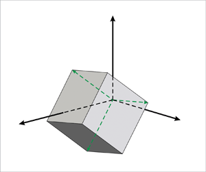
 $\chi$, known as the Euler angle. Both of these quantities are the invariants of the rotation matrix. Figure 1 shows the Euler angle and the Euler axis due to the relative rotation between the right-handed eigenframe of the SFS tensor, i.e.
 $\boldsymbol{\mathsf{V}}^{\boldsymbol {\tau }}$ with respect to the eigenframe of the FSR tensor, i.e.
 $\boldsymbol{\mathsf{V}}^{\boldsymbol{s}}$. As can be seen from this figure, the orientation of the Euler axis
 $\boldsymbol {q}$ can be quantified in terms of its colatitude angle
 $\theta =\cos ^{-1}(\boldsymbol {q}\boldsymbol {\cdot }\boldsymbol {v}^{\boldsymbol {s}}_{\gamma })$ and its longitude angle
 $\phi =\cos ^{-1}[(\boldsymbol {q} - \boldsymbol {q}\bot )\boldsymbol {\cdot }\boldsymbol {v}^{\boldsymbol {s}}_{\alpha }]$, in which
 $\boldsymbol {q}\bot \equiv (\boldsymbol {q}\boldsymbol {\cdot } \boldsymbol {v}^{\boldsymbol {s}}_{\gamma })\boldsymbol {v}^{\boldsymbol {s}}_{\gamma }$.
Relative rotation between the right-handed eigenframes of the SFS and FSR tensors based on the Euler rotation angle  $\chi$ and Euler axis
 $\boldsymbol {q}$. The Euler axis can be specified by colatitude and longitude angles, (
 $\theta, \phi$). The axes are eigenvectors of the FSR and SFS tensors (for example,
 $\boldsymbol {v}^{\boldsymbol {s}}_\alpha$ denotes the eigenvector of
 $\tilde {\boldsymbol{\mathsf{s}}}$ that corresponds to the eigenvalue
 $\alpha$).

However, it should be noted that the rotation matrix is directly related to  $\boldsymbol{\mathsf{V}}^{\boldsymbol {\tau }}$ and
 $\boldsymbol{\mathsf{V}}^{\boldsymbol{s}}$, which are subjected to directional aliasing since the directions of their eigenvectors are ambiguous by definition; that is, both
 $\boldsymbol {v}_\alpha$ and
 $\boldsymbol {-v}_\alpha$ eigenvectors are associated with the same eigenvalue
 $\alpha$. Therefore, corresponding to the FSR eigenvalues,
 $|\alpha ^s|\geq |\beta ^s|\geq |\gamma ^s|$, there are four possible right-handed eigenframes
 $\boldsymbol{\mathsf{V}}^{\boldsymbol{s}}$, namely,
 $[ \boldsymbol {v}^{\boldsymbol {s}}_{\alpha }, \boldsymbol {v}^{\boldsymbol {s}}_{\beta }, \boldsymbol {v}^{\boldsymbol {s}}_{\gamma }]$,
 $[ \boldsymbol {v}^{\boldsymbol {s}}_{\alpha }, -\boldsymbol {v}^{\boldsymbol {s}}_{\beta },-\boldsymbol {v}^{\boldsymbol {s}}_{\gamma }]$,
 $[-\boldsymbol {v}^{\boldsymbol {s}}_{\alpha }, \boldsymbol {v}^{\boldsymbol {s}}_{\beta },-\boldsymbol {v}^{\boldsymbol {s}}_{\gamma }]$ and
 $[-\boldsymbol {v}^{\boldsymbol {s}}_{\alpha }, -\boldsymbol {v}^{\boldsymbol {s}}_{\beta }, \boldsymbol {v}^{\boldsymbol {s}}_{\gamma }]$. Similarly, for the SFS eigenframe, i.e.
 $\boldsymbol{\mathsf{V}}^{\boldsymbol {\tau }}$, the same four possibilities exist:
 $[ \boldsymbol {v}^{\boldsymbol {\tau }}_{\alpha }, \boldsymbol {v}^{\boldsymbol {\tau }}_{\beta }, \boldsymbol {v}^{\boldsymbol {\tau }}_{\gamma }]$,
 $[ \boldsymbol {v}^{\boldsymbol {\tau }}_{\alpha }, -\boldsymbol {v}^{\boldsymbol {\tau }}_{\beta },-\boldsymbol {v}^{\boldsymbol {\tau }}_{\gamma }]$,
 $[-\boldsymbol {v}^{\boldsymbol {\tau }}_{\alpha }, \boldsymbol {v}^{\boldsymbol {\tau }}_{\beta },-\boldsymbol {v}^{\boldsymbol {\tau }}_{\gamma }]$ and
 $[-\boldsymbol {v}^{\boldsymbol {\tau }}_{\alpha }, -\boldsymbol {v}^{\boldsymbol {\tau }}_{\beta }, \boldsymbol {v}^{\boldsymbol {\tau }}_{\gamma }]$. Correspondingly, the relative orientation of the Euler axis,
 $\boldsymbol {q}$, with respect to the four possible eigenframes
 $\boldsymbol{\mathsf{V}}^{\boldsymbol {s}}$ are
 $(\theta,\phi )$,
 $(180^{\circ }-\theta,-\phi )$,
 $(180^{\circ }-\theta,180^{\circ }-\phi )$ and
 $(\theta,\phi -180^{\circ })$, respectively (see figure 2 in Yang & Wang (Reference Yang and Wang2016)). Therefore, for a randomly selected eigenframe
 $\boldsymbol{\mathsf{V}}^{\boldsymbol{s}}$, the statistical distribution of the Euler axis, which is expressed in terms of the joint probability density function (j.p.d.f.) of
 $(\theta,\phi )$, shows identical probabilities for all four scenarios, i.e.
 \begin{equation} P(\theta,\phi)=P(180^{{\circ}}-\theta,-\phi)=P(180^{{\circ}}-\theta,180^{{\circ}}-\phi)=P(\theta,\phi-180^{{\circ}}). \end{equation}
As a result of this directional ambiguity, which is expressed in terms of the statistical distribution (2.10), the most probable state of the Euler axis orientation can be aliased by these four possibilities. To remove this ambiguity, among these different possibilities, the absolute and the relative eigenframes are those eigenframes in which  $\theta \in [0^\circ, 90^\circ ]$ and
 $\phi \in [-90^\circ, 90^\circ ]$ (Wang et al. Reference Wang, Yee and Bergstrom2006; Yang & Wang Reference Yang and Wang2016).
Having uniquely determined the appropriate eigenframes  $\boldsymbol{\mathsf{V}}^{\boldsymbol {\tau }}$ and
 $\boldsymbol{\mathsf{V}}^{\boldsymbol{s}}$, the Euler angle
 $\chi$ can be determined based on the Rodrigues’ rotation formula:
 \begin{equation} \chi =\cos^{{-}1}\frac{\mathrm{tr}(\boldsymbol{\mathsf{R}})-1}{2}. \end{equation}
Correspondingly, the Euler axis  $\boldsymbol {q} = [q_1, q_2, q_3]^\textrm {T}$ is determined from the skew-symmetric part of the rotation matrix as
 \begin{equation} \boldsymbol{\mathsf{q}}^{{\times}} =\frac{\boldsymbol{\mathsf{R}}^T-\boldsymbol{\mathsf{R}}}{2\sin(\chi)}, \end{equation}
where  $\boldsymbol{\mathsf{q}}^{\times }$ represents the following skew-symmetric matrix:
 \begin{equation} \boldsymbol{\mathsf{q}}^{{\times}} = \begin{pmatrix} 0 & -q_3 & q_2 \\ q_3 & 0 & -q_1 \\ -q_2 & q_1 & 0 \end{pmatrix}. \end{equation}
Based on the statistics of these angles, i.e.  $(\chi,\theta,\phi )$, the relative attitude between FSR and SFS is analysed in following sections.
3. Results and discussion
3.1. Direct numerical simulation data set
To investigate the geometrical statistics of SFEF based on different filter functions, the direct numerical simulation (DNS) of a forced homogeneous isotropic turbulence is considered. The flow field results of the DNS are obtained from the Johns Hopkins Turbulence Database (JHTDB), whose simulation details can be found on the JHTDB website (Perlman et al. Reference Perlman, Burns, Li and Meneveau2007; Li et al. Reference Li, Perlman, Wan, Yang, Meneveau, Burns, Chen, Szalay and Eyink2008; Minping et al. Reference Minping, Chen, Eyink, Meneveau, Johnson, Perlman, Burns, Li, Szalay and Hamilton2012). Briefly, the incompressible Navier–Stokes equation is solved using the pseudospectral algorithm in a cubic domain of size  $L=2{\rm \pi}$ with periodic boundary conditions, discretized by
 $1024^3$ grid points. The nonlinear terms of the Navier–Stokes equation are dealiased using the combined phase-shift and
 $2\sqrt {2} /3$ truncation methods. Therefore, the effective spectral resolution is
 $k_{max}\eta \approx 1.35$, where
 $k_{max}$ is the highest wavenumber,
 $\eta$ is the Kolmogorov length scale and
 $\eta /L\approx 5\times 10^{-5}$. At the supergrid scale, forcing is applied to all modes within the spectral radius
 $k\eta \lesssim 6\times 10^{-3}$, i.e. shells with
 $k\leq 2$. This forcing maintains the turbulent flow stationary at the Taylor microscale Reynolds number of
 ${Re}_{\lambda } \approx 433$.
Figure 2 presents the volume-averaged SFEF as a function of the filter width  $k={\rm \pi} /\varDelta$ based on the
 $\mathcal {S}$- and
 $\mathcal {G}$-filtering methods, namely,
 $\langle \varPi _\mathcal {S}\rangle$ and
 $\langle \varPi _\mathcal {G}\rangle$ (the subscripts
 $\mathcal {S}$ and
 $\mathcal {G}$ represent the corresponding filter functions). Consistent with the previously reported findings (Rivera, Aluie & Ecke Reference Rivera, Aluie and Ecke2014; Buzzicotti et al. Reference Buzzicotti, Linkmann, Aluie, Biferale, Brasseur and Meneveau2018; Alexakis & Chibbaro Reference Alexakis and Chibbaro2020), it can be observed that
 $\langle \varPi _\mathcal {G}\rangle$ shows smoother variation with wavenumber
 $k={\rm \pi} /\varDelta$ compared with
 $\langle \varPi _\mathcal {S}\rangle$. This difference stems from the non-trivial contribution of the non-local interactions in the
 $\mathcal {S}$-filtering as follows.
The SFEF based on the  $\mathcal {S}$-filtering
 $\langle \varPi _\mathcal {S} \rangle$ and
 $\mathcal {G}$-filtering
 $\langle \varPi _\mathcal {G} \rangle$, as a function of the filter width
 $k={\rm \pi} /\varDelta$, normalized by the total turbulent kinetic energy dissipation rate,
 $\epsilon$.

Consider the non-local triadic interaction  $\boldsymbol {r}+\boldsymbol {p}+\boldsymbol {q}=0$, in which two coupling modes are in the neighbourhood of the spectral shell boundary
 $k={\rm \pi} /\varDelta$, say
 $r\ll p\approx {\rm \pi}/\Delta \approx q$ with mode
 $p(q)$ just below(above)
 $k$. In
 $\mathcal {G}$-filtering with the filter threshold
 $k$, due to the spectral overlap of the adjacent modes
 $p\approx q$, their corresponding triadic interaction cannot survive, and consequently, their coupling is averaged out. This situation contrasts the
 $\mathcal {S}$-filtering, in which the coupling modes
 $p\approx q$ are separated by a sharp boundary, and their interaction can contribute to the SFEF through its corresponding triadic interaction. Besides the contribution of the non-local interactions, some part of the energy flux in
 $\mathcal {S}$-filtering appears as the spatial energy transport of the subfilter scales in
 $\mathcal {G}$-filtering approach (see schematic 7 in Piomelli et al. (Reference Piomelli, Cabot, Moin and Lee1991)).
In the following, the impact of different filtering approaches, namely,  $\mathcal {S}$- and
 $\mathcal {G}$-filtering, on the SFEF is further investigated in terms of their statistical geometry. The filter size used throughout the present research corresponds to
 $k\eta \approx 0.11$, which is located in the plateau region of the energy flux in figure 2. Interestingly, the results do not show sensitive dependence on the filter width, and changing the filter size over
 $k\eta \in [0.02,0.2]$ does not show any significant effect on the results.
3.2. Relative attitude
In this section, the impact of different filtering approaches on the relative eigenframe alignment between FSR and SFS tensors is investigated. The main statistical parameters of the eigenframe alignment are presented in table 1. Interestingly, it can be observed that for both  $\mathcal {S}$-filter and
 $\mathcal {G}$-filter,
 $\langle \chi \rangle$,
 $\langle \theta \rangle$ and
 $\langle \phi \rangle$ show similar values. Therefore, the filter type does not considerably influence the average alignment between the FSR and SFS eigenframes. However, it will be seen that despite the similar mean behaviour, the statistical distribution of the eigenframe alignment shows a sensitive dependence on the filter kernel. In the following, the statistical distributions of the Euler angle,
 $\chi$, and Euler axis orientation,
 $(\theta, \phi )$, are investigated.
Statistics of the Euler angle,  $\chi$, and Euler axis orientation,
 $(\theta, \phi )$, for
 $\mathcal {G}$- and
 $\mathcal {S}$-filters.

3.2.1. Euler angle (rotation angle)
Figure 3 demonstrates the p.d.f. of the Euler angle,  $P(\chi )$, based on the
 $\mathcal {G}$-filter and
 $\mathcal {S}$-filter. Although
 $\chi \in [0^{\circ }, 180^{\circ }]$, it can be seen that for both filter functions, the probability for
 $\chi =0^\circ$ and
 $\chi \geq 120^\circ$ are zero. The first zero probability, namely,
 $P(\chi =0^\circ )=0$, indicates that the SFS eigenframe is rarely in alignment with the FSR eigenframe.
Density function (p.d.f.) of the Euler angle,  $P(\chi )$, based on the
 $\mathcal {G}$-filtering and
 $\mathcal {S}$-filtering.

Before comparing the p.d.f. of the Euler angle for the  $\mathcal {S}$- and
 $\mathcal {G}$-filtering methods, it is worth providing some physical intuition about the specific values of the Euler angle. Considering an archetype flow configuration, consisting of a compression–elongation flow accompanied by a shear motion, it can be shown that the Euler angles
 $\chi =45^{\circ }$,
 $90^{\circ }$ and
 $120^{\circ }$ can be related to the strong and weak shear motions. Under dominant shear conditions, the alignment between SFS and the FSR eigenframes is through a
 $\chi =45^{\circ }$ rotation angle. On the other hand, in weak shear conditions, the Euler angle can hold either
 $90^{\circ }$ or
 $120^{\circ }$ depending on the ratio of compression–elongation of the FSR tensor. If this ratio is within
 $[1/2 , 2]$ range, which is an almost isotropic compression, the Euler angle is
 $\chi = 90^{\circ }$. If this ratio exhibits more anisotropic distribution, i.e. the ratio increases as
 $[2 , \infty ]$, the Euler angle jumps to
 $\chi = 120^{\circ }$ (see Yang & Wang (Reference Yang and Wang2016) for more details).
Considering the fact that for both filters in figure 3, the Euler angle  $\chi = 90^{\circ }$ is the most probable state and
 $\chi \geq 120^{\circ }$ has zero probability, it indicates that isotropic compression is the most probable state in both filtering formulations, while anisotropic compression rarely happens. Despite these similarities,
 $P(\chi )$ for the two filtering approaches shows non-trivial differences as follows.
In  $\mathcal {G}$-filtering,
 $P(\chi )$ exhibits a bimodal behaviour with a primary mode at
 $\chi =90^\circ$ and a secondary mode at
 $\chi =45^\circ$. This bimodal pattern has also been reported in a previous study (Yang & Wang Reference Yang and Wang2016) based on the box filter, which is similar to the
 $\mathcal {G}$-filter, a non-projector filter. On the other hand,
 $P(\chi )$ for the
 $\mathcal {S}$-filtering does not have a local maximum at
 $\chi =45^\circ$, while it shows a higher probability for
 $75\,^\circ \leq \chi \leq 90^\circ$ rotation angle range compared with the
 $\mathcal {G}$-filtering.
Therefore, in contrast to the  $\mathcal {G}$-filtering, in which both weak and strong shear motions show high probability, the
 $\mathcal {S}$-filtering effectively annihilates the strong shear motion while having an augmentation effect on the normal straining motion. However, despite this different statistical distribution, the average value of the Euler angle for both filters is identical,
 $\langle \chi \rangle = 64^{\circ }$, as presented in table 1.
3.2.2. Euler axis (rotation axis)
The orientation of the Euler axis  $\boldsymbol {q}$ is specified by the colatitude angle
 $\theta \in [0^\circ, 90^\circ ]$ and the longitude angle
 $\phi \in [-90^\circ, 90^\circ ]$. Here, the Euler axis statistics are shown in terms of the premultiplied j.p.d.f.s of these angles, i.e.
 $P_m(\theta,\phi )\equiv P(\theta,\phi )\sin \theta$, in which
 $\sin \theta$ ensures an unbiased probability distribution for the randomly oriented
 $\boldsymbol {q}$ with uniform probability distribution (Higgins et al. Reference Higgins, Parlange and Meneveau2003; Yang & Wang Reference Yang and Wang2016).
Figure 4 presents  $P_m(\theta,\phi )$ based on the
 $\mathcal {G}$- and
 $\mathcal {S}$-filtering. These j.p.d.f.s are obtained by dividing the whole range of
 $\theta$ and
 $\phi$ into
 $50\times 50$ identical bins. Figure 4(a) shows that the most probable orientation of the Euler axis for
 $\mathcal {G}$-filtering is
 $(\theta,\phi )\approx (65^\circ,17^\circ )$, which is consistent with the previously reported result
 $(\theta,\phi )\approx (62^\circ,15^\circ )$ based on the box filtering (Yang & Wang Reference Yang and Wang2016). On the other hand, figure 4(b) shows that
 $P_m(\theta,\phi )$ based on the
 $\mathcal {S}$-filtering has a pronounced bimodal distribution, which is qualitatively different from the
 $\mathcal {G}$-filtering. This bimodal shape of
 $P_m(\theta,\phi )$ shows an approximately symmetric distribution of the most probable states at
 $(\theta,\phi )\approx (90^\circ,\pm 45^\circ )$ with equal probabilities. It will be seen that this symmetrical distribution of the rotation axis in the
 $\mathcal {S}$-filtering approach has a non-trivial effect on the forward–backward energy flux cancellation.
Statistics of the Euler axis orientation based on the premultiplied j.p.d.f. of the colatitude and longitude angles,  $P_m(\theta,\phi )$, for (a) a
 $\mathcal {G}$-filter, and (b) an
 $\mathcal {S}$-filter.

Based on these statistics, the most probable relative attitudes between the FSR and SFS eigenframes are visualized in figure 5, while more quantitative information is compiled in Appendix A, figure 12. Interestingly, in contrast to table 1 which shows that the mean alignment, i.e.  $\langle \chi \rangle$,
 $\langle \theta \rangle$ and
 $\langle \phi \rangle$, are almost identical for both
 $\mathcal {S}$- and
 $\mathcal {G}$-filters, figure 5 shows that the most probable alignments between
 ${\tilde {\boldsymbol{\mathsf{s}}}}$ and
 $\boldsymbol {\tau }$ are quite different.
Schematic of the most probable eigenframes of the FSR, denoted by black  $\boldsymbol {v}^{\boldsymbol {s}}_\alpha$–
 $\boldsymbol {v}^{\boldsymbol {s}}_\beta$–
 $\boldsymbol {v}^{\boldsymbol {s}}_\gamma$ axes, and the SFS eigenframe, visualized on the edges of a cube with red axes
 $\boldsymbol {v}^{\boldsymbol {\tau }}_\alpha$–
 $\boldsymbol {v}^{\boldsymbol {\tau }}_\beta$–
 $\boldsymbol {v}^{\boldsymbol {\tau }}_\gamma$. The most probable state of
 $(\theta, \phi,\chi )$ for
 $\mathcal {G}$-filter at (a)
 $(65^\circ,17^\circ,90^\circ )$ (G1), and (b)
 $(65^\circ,17^\circ,45^\circ )$ (G2). The most probable state of
 $(\theta, \phi,\chi )$ for
 $\mathcal {S}$-filter at (c)
 $(80^\circ, -45^\circ,90^\circ )$ (S1), and (d
 $(80^\circ, 45^\circ,90^\circ )$ (S2).

Figures 5(a) and 5(b) show the primary and the secondary configurations based on the  $\mathcal {G}$-filtering, i.e.
 $(\theta, \phi,\chi ) \approx (65^\circ,17^\circ,90^\circ )$ and
 $(65^\circ,17^\circ,45^\circ )$, respectively. By comparing these two configurations, it can be seen that in the primary mode, the eigenvectors
 $\boldsymbol {v}^{\boldsymbol {s}}_{\beta }$ and
 $\boldsymbol {v}^{\boldsymbol {\tau }}_{\gamma }$ show a pronounced alignment, while this strong alignment cannot be observed in the secondary mode. However, in both primary and secondary configurations, the alignment between
 $(\boldsymbol {v}^{\boldsymbol {s}}_{\alpha },\boldsymbol {v}^{\boldsymbol {\tau }}_{\alpha })$ eigenvectors is more pronounced compared with
 $(\boldsymbol {v}^{\boldsymbol {s}}_{\beta },\boldsymbol {v}^{\boldsymbol {\tau }}_{\beta })$, and
 $(\boldsymbol {v}^{\boldsymbol {s}}_{\gamma },\boldsymbol {v}^{\boldsymbol {\tau }}_{\gamma })$ (this issue can also be observed quantitatively in figure 12a,e,i by considering the columns G1 and G2). As will be discussed shortly, the alignment between (
 $\boldsymbol {v}^{\boldsymbol {s}}_{\alpha }$,
 $\boldsymbol {v}^{\boldsymbol {\tau }}_{\alpha }$) eigenvectors has an augmentation effect on the forward energy transfer of SFEF based on the
 $\mathcal {G}$-filtering.
Figures 5(c) and 5(d) show the most probable configurations in  $\mathcal {S}$-filtering, i.e.
 $(\theta, \phi,\chi ) \approx (80^\circ,\pm 45^\circ,90^\circ )$. It can be seen that in these cases, the eigenvectors corresponding to the smallest eigenvalues are perpendicular, i.e.
 $\boldsymbol {v}^{\boldsymbol {\tau }}_{\gamma } \perp \boldsymbol {v}^{\boldsymbol {s}}_{\gamma }$ (see columns S1 and S2 in figure 12i). However, concerning the interscale energy transfer, the most important point in configurations S1 and S2 is the relative alignment of
 $\boldsymbol {v}^{\boldsymbol {s}}_{\alpha }$ with
 $\boldsymbol {v}^{\boldsymbol {\tau }}_{\alpha }$ and
 $\boldsymbol {v}^{\boldsymbol {\tau }}_{\gamma }$. It can be observed that in both S1 and S2 configurations, the eigenvectors
 $\boldsymbol {v}^{\boldsymbol {s}}_{\alpha }$ and
 $\boldsymbol {v}^{\boldsymbol {\tau }}_{\alpha }$ are in the same direction, i.e.
 $(\boldsymbol {v}^{\boldsymbol {s}}_{\alpha }\boldsymbol {\cdot }\boldsymbol {v}^{\boldsymbol {\tau }}_{\alpha })>0$ (see also figure 12a, columns S1 and S2). On the other hand, the directional tendency between
 $\boldsymbol {v}^{\boldsymbol {s}}_{\alpha }$ and
 $\boldsymbol {v}^{\boldsymbol {\tau }}_{\gamma }$ shows different behaviours:
 $(\boldsymbol {v}^{\boldsymbol {s}}_{\alpha }\boldsymbol {\cdot }\boldsymbol {v}^{\boldsymbol {\tau }}_{\gamma })$ is positive in S1, while it is negative in S2 (see also figure 12c, columns S1 and S2). It will be shortly seen that this behaviour has a hampering effect on the forward energy transfer based on the
 $\mathcal {S}$-filtering.
3.3. Geometrical structure
In this section, the impact of different filtering approaches on the eigenstructures of the FSR and SFS is analysed in terms of a non-dimensional state parameter,  $s^*$. Considering the FSR tensor, this non-dimensional parameter, known as the strain-state parameter, is defined as (Lund & Rogers Reference Lund and Rogers1994)
 \begin{equation} s^* = \frac{-3\sqrt{6}\alpha_s \beta_s \gamma_s}{(\alpha^2_s + \beta^2_s + \gamma^2_s)^{3/2}}, \end{equation}
where  $\alpha _s$,
 $\beta _s$ and
 $\gamma _s$ are eigenvalues of the FSR tensor. Considering the fact that the incompressible strain rate is a deviatoric tensor, this parameter lies in the range
 $[-1,1]$ and a random velocity field displays a uniform p.d.f. for
 $s^*$.
To provide some physical intuition for  $s^*$, this parameter is mainly interpreted as a measure of the geometrical character of the local deformations caused by the strain rate. Accordingly, the plane shear corresponds to
 $s^*=0$, while in axisymmetric extension and contraction,
 $s^*=1$ and
 $s^*=-1$, respectively. A schematic of the deformation topology for an initially spherical fluid particle is depicted in the upper part of figure 6(c). It is also found that for an isotropic turbulence, the most probable value of strain-state is axisymmetric extension and this state is well correlated with regions of high dissipation rate (Lund & Rogers Reference Lund and Rogers1994).
Impact of the filter kernel on the eigenstructure of the FSR and SFS tensors. The p.d.f. of (a) the strain-state,  $P(s^*)$, and (b) the stress-state,
 $P(\tau ^*)$. (c) Functional relation between the normalized eigenvalues,
 $\alpha ^*$ (Red),
 $\beta ^*$ (Green),
 $\gamma ^*$ (Blue) and corresponding state parameter, i.e. relations (3.3). The upper part of (c) provides axisymmetric contraction
 $s^*=-1$, plane shear
 $s^*=0$, and axisymmetric extension
 $s^*=1$ for an initially spherical fluid particle.

Similarly, expression (3.1) can also be extended for geometrically characterizing the SFS tensor by defining the stress-state parameter,  $\tau ^*$ (Tao et al. Reference Tao, Katz and Meneveau2002; Higgins et al. Reference Higgins, Parlange and Meneveau2003) as
 \begin{equation} \tau^* = \frac{-3\sqrt{6}\alpha_\tau \beta_\tau \gamma_\tau}{(\alpha^2_\tau + \beta^2_\tau + \gamma^2_\tau)^{3/2}}, \end{equation}
where  $\alpha _\tau$,
 $\beta _\tau$ and
 $\gamma _\tau$ are eigenvalues of the deviatoric part of the SFS tensor
 $\tau ^d_{ij} = \tau _{ij} - 1/3 \tau _{kk}\delta _{ij}$. Similar to
 $s^*$, the value of
 $\tau ^*$ is also in the interval
 $[-1,1]$, and it yields a uniform p.d.f. for a random velocity field. A unique dependence between the normalized eigenvalues and the state parameter exists as (Lund & Rogers Reference Lund and Rogers1994)
 \begin{equation} \left.\begin{gathered} \alpha^* ={-}\cos \varPsi + \sqrt{3} |\sin \varPsi |\\ \beta^* = 2\cos \varPsi \\ \gamma^* ={-}\cos \varPsi - \sqrt{3} |\sin \varPsi |,\end{gathered}\right\} \end{equation}
where  $\alpha ^*$,
 $\beta ^*$ and
 $\gamma ^*$ are the eigenvalues normalized by
 $(\alpha ^2+\beta ^2+\gamma ^2)^{1/2}/\sqrt {6}$, e.g.
 $\beta ^* = \sqrt {6}\beta /(\alpha ^2+\beta ^2+\gamma ^2)^{1/2}$. Moreover, the angle parameter is defined as
 $\varPsi = 5/3{\rm \pi} - 1/3 \cos ^{-1}(\bullet )$, in which
 $(\bullet )$ stands for the corresponding state parameter
 $s^*$ or
 $\tau ^*$.
The main statistics of  $s^*$ and
 $\tau ^*$ are gathered in table 2, while figure 6 provides their statistical distributions as well as their eigenstructures. Figure 6(a) presents the p.d.f. of the strain-state parameter,
 $s^*$, based on the
 $\mathcal {S}$-filter and
 $\mathcal {G}$-filter. It can be observed that for both filter kernels,
 $P(s^*)$ shows almost similar distribution with the most likely state at
 $s^* \to 1$, corresponding to the local axisymmetric extension. This similar statistical distribution of
 $s^*$ for the two filters can also be quantitatively recovered from their approximately equal mean values and variances, presented in table 2. Therefore, it can be asserted that different filtering approaches do not significantly affect the eigenstructure of the FSR tensor.
Statistics of the strain-state parameter  $s^*$ and the stress-state parameter
 $\tau ^*$ (for the
 $\mathcal {S}$-filter, the mean value
 $\langle \tau ^* \rangle =-0.004$ is presented by
 $-0.00$).

The eigenstructure of the FSR tensor can be further analysed from relations (3.3), which is visualized in figure 6(c). Considering the most probable strain-state  $s^* \to 1$, figure 6(c) shows that the most probable eigenstructure of FSR tends to be
 $\alpha ^*_s : \beta ^*_s : \gamma ^*_s = 1 : 1 : -2$. Therefore, for both filtering formulations, the descending order based on the absolute values is
 $|\gamma _s|\geq |\alpha _s| \geq |\beta _s|$, which corresponds to the contractive–extensive–intermediate eigenvectors (note that
 $\alpha >0$,
 $\beta$ and
 $\gamma <0$, correspond to the extensive, intermediate and contractive eigendirections, respectively).
Figure 6(b) presents the p.d.f. for the stress-state parameter  $\tau ^*$. It can be observed that in contrast to the FSR tensor, different filtering approaches have a non-trivial impact on the eigenstructure of the SFS tensor. Here
 $P(\tau ^*)$ in the
 $\mathcal {G}$-filtering shows the most likely state for the axisymmetric contraction,
 $\tau ^* \to -1$, while in
 $\mathcal {S}$-filtering,
 $P(\tau ^*)$ shows a uniform distribution corresponding to a random field with a negligible mean value,
 $\langle \tau ^* \rangle \approx 0$, as presented in table 2.
Considering the most likely state  $\tau ^* \to -1$ for the SFS based on the
 $\mathcal {G}$-filtering, figure 6(c) implies that the most probable eigenstructure tends to be
 $\alpha ^*_\tau : \beta ^*_\tau : \gamma ^*_\tau = 2 : -1 : -1$. Therefore, in
 $\mathcal {G}$-filtering formulation, the descending order based on the absolute values is
 $|\alpha _\tau |\geq |\gamma _\tau | \geq |\beta _\tau |$ corresponding to extensive–contractive–intermediate eigenvectors.
On the other hand, uniform distribution of  $P(\tau ^*)$ for the SFS based on the
 $\mathcal {S}$-filtering implies
 $\alpha ^*_\tau : \beta ^*_\tau : \gamma ^*_\tau = 1.7 : 0 : -1.7$. Therefore, the descending order based on the absolute values is
 $|\alpha _\tau |= |\gamma _\tau |> |\beta _\tau |$, corresponding to contractive–extensive–intermediate eigenvectors. This specific eigenstructure is probably a direct consequence of the symmetrical distribution
 $\phi \approx \pm 45^\circ$, presented in figure 4.
3.4. Normalized energy flux
The impact of different filtering approaches on the SFEF can be investigated in terms of the normalized energy flux,
 \begin{equation} \varPi^* = \frac{-\tau^d_{ij}{\mathsf{s}}_{ij}}{(\tau^d_{mn}\tau^d_{mn})^{1/2}({\mathsf{s}}_{kl}{\mathsf{s}}_{kl})^{1/2}}, \end{equation}
which is bounded in the range  $[-1,1]$. The positive/negative value of
 $\varPi ^*$ reflects the forward–backward scatter energy transfer. In the following, the normalized energy fluxes based on the
 $\mathcal {S}$- and
 $\mathcal {G}$-filtering methods are denoted by their corresponding subscripts, namely,
 $\varPi ^*_\mathcal {S}$ and
 $\varPi ^*_\mathcal {G}$.
Figure 7 displays different statistical distributions of the normalized energy flux based on the  $\mathcal {G}$- and
 $\mathcal {S}$-filters. Figure 7(a) presents the j.p.d.f. based on the
 $\mathcal {G}$-filtering,
 $P(\varPi _\mathcal {G}^*,\chi )$. It can be seen that
 $P(\varPi _\mathcal {G}^*,\chi )$ exhibits three preferential modes corresponding to
 $(\varPi _\mathcal {G}^*,\chi )\approx (0.29,45^\circ )$,
 $(0.35,64^\circ )$ and
 $(0.43 , 90^\circ )$. Two modes
 $(0.29,45^\circ )$ and
 $(0.43 , 90^\circ )$ are associated with the most probable Euler angles
 $45^\circ$ and
 $90^\circ$, i.e. strong and weak shear conditions, respectively. The third mode
 $(0.35,64^\circ )$ is related to the average Euler angle
 $\langle \chi \rangle =64^\circ$, for the
 $\mathcal {G}$-filtering (see table 1). It can be seen that
 $P(\varPi _\mathcal {G}^*,\chi )$ is predominantly distributed over the
 $\varPi _\mathcal {G}^*> 0$ region which corresponds to the forward energy transfer.
Statistical distribution of the normalized energy flux,  $P(\varPi ^*,\chi )$, based on the (a)
 $\mathcal {G}$-filter, and (b)
 $\mathcal {S}$-filter. (c) The p.d.f. of
 $\varPi ^*$ for
 $\mathcal {G}$-filter and
 $\mathcal {S}$-filter.

Figure 7(b) presents the same j.p.d.f. based on the  $\mathcal {S}$-filtering, i.e.
 $P(\varPi _\mathcal {S}^*,\chi )$. In contrast to the
 $\mathcal {G}$-filtering, it can be observed that the most probable state of
 $(\varPi _\mathcal {S}^*,\chi )$ shows a single-mode pattern at
 $(\varPi _\mathcal {S}^*,\chi )\approx (0,90^\circ )$, corresponding to the most probable Euler angle
 $\chi =90^\circ$ in figure 3. However, the statistical distribution of
 $\varPi _\mathcal {S}^*$ shows a non-trivial difference compared with that of
 $\varPi _\mathcal {G}^*$: while the distribution of
 $P(\varPi _\mathcal {G}^*,\chi )$ is predominantly in the forward (positive) flux region,
 $P(\varPi _\mathcal {S}^*,\chi )$ shows an almost symmetrical distribution over both forward–backward flux regions.
This different statistical distribution of the normalized energy transfer for the  $\mathcal {S}$- and
 $\mathcal {G}$-filters can be better demonstrated in terms of their overall p.d.f.s, i.e.
 $P(\varPi _\mathcal {S}^*)$ and
 $P(\varPi _\mathcal {G}^*)$, which are presented in figure 7(c). First, it can be observed that the filter type does not considerably influence the most probable value of the normalized energy flux, i.e.
 $\varPi _\mathcal {G}^*=0.38$ and
 $\varPi _\mathcal {S}^*=0.30$. However, the statistical distribution of the normalized energy transfer,
 $P(\varPi ^*)$, is significantly affected by the filter type:
 $P(\varPi _\mathcal {G}^*)$ is skewed towards the positive region
 $\varPi _\mathcal {G}^*>0$, and is concentrated around its most probable value
 $\varPi _\mathcal {G}^*=0.38$ with forward mean normalized energy transfer
 $\langle \varPi _\mathcal {G}^* \rangle = 0.28$. On the other hand,
 $P(\varPi _\mathcal {S}^*)$ exhibits an almost symmetrical distribution over both positive and negative flux regions
 $\varPi _\mathcal {S}^* \gtrless 0$. As a result of this nearly symmetrical distribution, significant cancellation occurs between forward and backward energy transfer, leading to a considerably smaller mean normalized energy flux in
 $\mathcal {S}$-filtering,
 $\langle \varPi _\mathcal {S}^* \rangle = 0.08$, compared with that in
 $\mathcal {G}$-filtering.
This issue can be further investigated by considering the forward–backward components of the energy flux,
 \begin{equation} \varPi^\pm = \tfrac{1}{2}(\varPi \pm |\varPi|). \end{equation}
The contribution of these forward–backward scatter energy fluxes to the overall SFEF can be quantified by  $\varepsilon \equiv \varPi /(\varPi ^+ - \varPi ^-)=\varPi /|\varPi |$, which equals
 $+1(-1)$ in regions with
 $\varPi >0(\varPi <0)$ (note that this parameter,
 $\varepsilon$, should not be confused with the dissipation rate, which is mainly denoted by
 $\epsilon$).
Figure 8 shows the p.d.f. of  $\varepsilon$,
 $P(\varepsilon )$, obtained based on
 $\mathcal {S}$- and
 $\mathcal {G}$-filtering approaches. Obviously, for both
 $\varPi _\mathcal {S}$ and
 $\varPi _\mathcal {G}$, this parameter shows a double-Delta-function distribution
 $P(\varepsilon )=f\delta (\varPi -\varPi ^-)+ (1-f)\delta (\varPi -\varPi ^+)$, where
 $f$ is the probability of the backscatter energy fluxes. It is found that for the
 $\mathcal {G}$-filter
 $f=0.17$, while for the
 $\mathcal {S}$-filter
 $f=0.42$, i.e. the backscatter fraction in
 $\varPi _\mathcal {S}$ is almost 2.5 times larger than that in
 $\varPi _\mathcal {G}$.
The p.d.f. of  $\varepsilon \equiv \varPi /(\varPi ^+ - \varPi ^-)$ based on the
 $\mathcal {S}$-filter and
 $\mathcal {G}$-filter.

This relatively large backscatter fraction in  $\mathcal {S}$-filtering, which leads to a substantial cancellation among the forward–backward energy transfers, will be discussed in the following sections. However, it is worth comparing this observation with the previously reported results. In a turbulent channel flow, the SFEF based on the
 $\mathcal {G}$- and
 $\mathcal {S}$-filters results in backscattering in approximately
 $30\,\%$ and
 $50\,\%$ of the grid points, respectively (Piomelli et al. Reference Piomelli, Cabot, Moin and Lee1990). Comparing this reported result for an anisotropic turbulence (channel flow) with the observed results in an isotropic turbulence (current research) prompts the conjuncture that a high backscatter fraction could be an intrinsic property of the
 $\mathcal {S}$-filtering.
3.5. Cancellation effect
In this section, the forward–backward energy flux cancellation is further investigated in terms of the relative eigenframe alignment. To this end, the normalized energy flux (3.4) is decomposed into different forward–backward partial energy fluxes as follows (Higgins et al. Reference Higgins, Parlange and Meneveau2004):
 \begin{align}
\varPi^* &= \frac{1}{6} \{\underbrace{(\boldsymbol{v}^{\boldsymbol{s}}_{\alpha} \boldsymbol{\cdot}
\boldsymbol{v}^{\boldsymbol \tau}_{\alpha})^2 (\beta^*_s -
\alpha^*_{s}) ( \alpha^*_{\tau} - \beta^*_{\tau}
)}_{\varPi^*_1<0} + \underbrace{(\boldsymbol{v}^{\boldsymbol{s}}_{\gamma}
\boldsymbol{\cdot} \boldsymbol{v}^
{\boldsymbol{\tau}}_{\gamma})^2 (\beta^*_{s} -\gamma^*_s)
(\gamma^*_{\tau} - \beta^*_{\tau})}_{\varPi^*_2<0}
\nonumber\\ &\quad+ \underbrace{(\boldsymbol{v}^{\boldsymbol{s}}_{\gamma}
\boldsymbol{\cdot}
\boldsymbol{v}^{\boldsymbol{\tau}}_{\alpha})^2 (\beta^*_{s}
-\gamma^*_s) (\alpha^*_{\tau} -
\beta^*_{\tau})}_{\varPi^*_3>0} +
\underbrace{(\boldsymbol{v}^{\boldsymbol{s}}_{\alpha} \boldsymbol{\cdot}
\boldsymbol{v}^{\boldsymbol{\tau}}_{\gamma})^2 (\beta^*_{s}
-\alpha^*_s) (\gamma^*_{\tau} -
\beta^*_{\tau})}_{\varPi^*_4>0} \nonumber\\ &\quad +
\underbrace{ 3\beta^*_{s}\beta^*_{\tau}}_{\varPi^*_5} \},
\end{align}
in which the eigenvalues are sorted as  $\alpha ^* \geq \beta ^* \geq \gamma ^*$. Note that unlike § 2.2 where the eigenframes are parameterized based on the absolute values of eigenvalues, here, the eigenvalues are sorted based on their values. According to this ordering of eigenvalues, the partial energy fluxes
 $\varPi ^*_1$ to
 $\varPi ^*_4$ are sign-definite and can be classified into forward (
 $\varPi ^*_3$ and
 $\varPi ^*_4$) and backward (
 $\varPi ^*_1$ and
 $\varPi ^*_2$ ) energy fluxes. Although the last partial flux, i.e.
 $\varPi ^*_5 =3\beta ^*_{s}\beta ^*_{\tau }$, is not sign-definite and can be either positive or negative, it is observed that on average,
 $\langle \varPi ^*_5\rangle <0$, and it contributes to the backward energy flux.
Figure 9 shows the averaged contribution of all partial fluxes,  $\langle \varPi ^*_1\rangle$ to
 $\langle \varPi ^*_5\rangle$, for both filtering formulations. As explained above, it can be seen that only
 $\langle \varPi ^*_3\rangle$ and
 $\langle \varPi ^*_4\rangle$ contribute to the forward energy transfer, while the rest of the partial fluxes are responsible for the backward energy transfer. However, the most striking point in figure 9 is the impact of the filter kernel on the partial energy fluxes. It can be seen that the mean partial fluxes
 $\langle \varPi ^*_1\rangle$,
 $\langle \varPi ^*_4\rangle$ and
 $\langle \varPi ^*_5\rangle$ do not show a significant dependence on the type of filter kernel. However, considering
 $\langle \varPi ^*_2 \rangle$ and
 $\langle \varPi ^*_3 \rangle$, this figure clearly shows that, compared with the
 $\mathcal {G}$-filtering, the
 $\mathcal {S}$-filtering has a hampering effect on the forward partial energy flux
 $\langle \varPi ^*_{\mathcal {S}3}\rangle <\langle \varPi ^*_{\mathcal {G}3}\rangle$, while augmenting the backward partial energy flux
 $|\langle \varPi ^*_{\mathcal {G}2}\rangle |<|\langle \varPi ^*_{\mathcal {S}2}\rangle |$ (note that, for example,
 $\varPi ^*_{\mathcal {G}2}$ denotes the partial energy flux
 $\varPi ^*_{2}$ based on the
 $\mathcal {G}$-filtering). Thus, the larger backscatter fraction in
 $\varPi _\mathcal {S}$ compared with
 $\varPi _\mathcal {G}$, observed in § 3.4, originates from different weights of the backward–forward partial energy fluxes, i.e.
 $\langle \varPi ^*_2\rangle$ and
 $\langle \varPi ^*_3\rangle$.
Contribution of different partial energy fluxes, i.e.  $\langle \varPi ^*_1\rangle$–
 $\langle \varPi ^*_5\rangle$ to the overall energy transfer based on the
 $\mathcal {S}$-filter and
 $\mathcal {G}$-filter.

The impact of different filter kernels on these forward–backward partial energy fluxes is further elaborated by considering their relations:
 \begin{equation} \left.\begin{gathered}
\varPi^*_2 = \tfrac{1}{6}
\underbrace{(\boldsymbol{v}^{\boldsymbol{s}}_{\gamma}
\boldsymbol{\cdot}
\boldsymbol{v}^{\boldsymbol{\tau}}_{\gamma})^2}_{{term~1}}
\underbrace{(\beta^*_{s}
-\gamma^*_{s})}_{{term~2}}
\underbrace{(\gamma^*_{\tau} -
\beta^*_{\tau})}_{{term~3}},
\\ \varPi^*_3 = \tfrac{1}{6}\underbrace{
(\boldsymbol{v}^{\boldsymbol{s}}_{\gamma}
\boldsymbol{\cdot}
\boldsymbol{v}^{\boldsymbol{\tau}}_{\alpha})^2}_{{term~1}}
\underbrace{(\beta^*_{s}
-\gamma^*_s)}_{{term~2}}
\underbrace{(\alpha^*_{\tau} -
\beta^*_{\tau})}_{{term~3}}.\end{gathered}\right\}
\end{equation}
It can be seen that these partial energy fluxes are functions of eigendirection alignments, i.e. term 1, and eigenstructures of FSR and SFS tensors, i.e. term 2 and term 3, respectively. Considering term 2 in these partial fluxes, it can be easily seen that this term is not affected by the filter type: the SFS eigenstructure is exclusively a function of the strain-rate parameter  $s^*$ (see (3.3)), and
 $P(s^*)$ is trivially affected by the filter type (see figure 6a). Therefore, the filter kernel can effectively modify
 $\langle \varPi ^*_2\rangle$ and
 $\langle \varPi ^*_3\rangle$ through the other two parameters, namely, term 1 and term 3.
Figure 10 shows the impact of the filter type on term 1 and term 3. The p.d.f.s of term 3 in  $\varPi _2^*$ and
 $\varPi _3^*$, viz.
 $(\gamma ^*_{\tau } - \beta ^*_{\tau })$ and
 $(\alpha ^*_{\tau } - \beta ^*_{\tau })$, are presented in figures 10(a) and 10(b). The statistical distributions of these two parameters clearly show that compared with
 $\mathcal {G}$-filtering,
 $(\gamma ^*_{\tau } - \beta ^*_{\tau })$ has a statistically larger value in
 $\mathcal {S}$-filtering, while
 $(\alpha ^*_{\tau } - \beta ^*_{\tau })$ shows the opposite statistical behaviour. Therefore, through the SFS eigenstructure, i.e. term 3, the
 $\mathcal {S}$-filtering augments the backward energy flux
 $\langle \varPi ^*_2\rangle$ while having a hampering effect on the forward energy flux
 $\langle \varPi ^*_3\rangle$.
Statistical distributions of the influential terms for two partial energy fluxes  $\varPi ^*_2$ and
 $\varPi ^*_3$ based on the
 $\mathcal {G}$-filtering and
 $\mathcal {S}$-filtering. p.d.f.s of (a) the eigenvalue difference
 $(\gamma ^*_{\tau } - \beta ^*_{\tau })$, (b) the eigenvalue difference
 $(\alpha ^*_{\tau } - \beta ^*_{\tau })$, (c) the alignment between contractive–contractive eigenvectors
 $(\boldsymbol{v}^{\boldsymbol{s}}_{\gamma } \boldsymbol {\cdot } \boldsymbol {v}^{\boldsymbol {\tau }}_{\gamma })$ and (d) the alignment between contractive–extensive eigenvectors
 $(\boldsymbol{v}^{\boldsymbol{s}}_{\gamma } \boldsymbol {\cdot } \boldsymbol {v}^{\boldsymbol {\tau }}_{\alpha })$.

Figures 10(c) and 10(d) present the impact of the filter kernel on the relevant eigenframe alignments in  $\varPi ^*_2$ and
 $\varPi ^*_3$, i.e. term 1. In figure 10(c), it can be seen that the alignment between the most contractive eigenvectors, i.e.
 $(\boldsymbol{v}^{\boldsymbol{s}}_{\gamma } \boldsymbol {\cdot } \boldsymbol {v}^{\boldsymbol {\tau }}_{\gamma })^2$, shows an almost identical statistical distribution in both
 $\mathcal {S}$- and
 $\mathcal {G}$-filtering. Therefore, the augmentation effect of the
 $\mathcal {S}$-filter on this backscatter partial flux, i.e.
 $|\langle \varPi ^*_{\mathcal {G}2}\rangle |<|\langle \varPi ^*_{\mathcal {S}2}\rangle |$, effectively originated from the increasing effect of this filter kernel on the eigenvalue difference
 $(\gamma ^*_{\tau } - \beta ^*_{\tau })$.
Figure 10(d) shows the alignment between contractive–extensive eigenvectors,  $(\boldsymbol{v}^{\boldsymbol{s}}_{\gamma } \boldsymbol {\cdot } \boldsymbol {v}^{\boldsymbol {\tau }}_{\alpha })^2$, based on the
 $\mathcal {S}$- and
 $\mathcal {G}$-filtering. Unlike eigendirection alignment
 $(\boldsymbol{v}^{\boldsymbol{s}}_{\gamma } \boldsymbol {\cdot } \boldsymbol {v}^{\boldsymbol {\tau }}_{\gamma })^2$, it can be observed that the filter kernel has a non-trivial impact on the alignment of contractive–extensive eigenvectors,
 $(\boldsymbol{v}^{\boldsymbol{s}}_{\gamma } \boldsymbol {\cdot } \boldsymbol {v}^{\boldsymbol {\tau }}_{\alpha })^2$. This figure shows that in
 $\mathcal {S}$-filtering, the most probable angle between the contractive–extensive eigenvectors is close zero, i.e.
 $(\boldsymbol{v}^{\boldsymbol{s}}_{\gamma } \boldsymbol {\cdot } \boldsymbol {v}^{\boldsymbol {\tau }}_{\alpha })\approx 0$, while the statistical distribution of this angle in
 $\mathcal {G}$-filtering shows a pronounced peak around
 $(\boldsymbol{v}^{\boldsymbol{s}}_{\gamma } \boldsymbol{\cdot} \boldsymbol {v}^{\boldsymbol {\tau }}_{\alpha })^2\approx 0.6$. Therefore, in addition to the larger eigenvalue difference
 $(\alpha ^*_{\tau } - \beta ^*_{\tau })$,
 $\mathcal {G}$-filtering can produce a more pronounced alignment between the contractive–extensive eigenvectors, resulting in a stronger partial forward flux compared with the
 $\mathcal {S}$-filtering, i.e.
 $\langle \varPi ^*_{\mathcal {S}3}\rangle < \langle \varPi ^*_{\mathcal {G}3}\rangle$. This impact of the filter type on the eigenframe alignment is further investigated in the next section.
3.6. Alignments of the contractive–extensive eigenvectors
In analysing the partial energy flux  $\varPi ^*_3$, it is observed that the most probable value of
 $(\boldsymbol{v}^{\boldsymbol{s}}_{\gamma } \boldsymbol {\cdot } \boldsymbol {v}^{\boldsymbol {\tau }}_{\alpha })$ in
 $\mathcal {G}$-filtering is considerably larger than that in
 $\mathcal {S}$-filtering. Here, we analyse the most preferential alignment between
 $\boldsymbol{v}^{\boldsymbol{s}}_{\gamma }$ and
 $\boldsymbol {v}^{\boldsymbol {\tau }}_{\alpha }$ in terms of the most probable state of Euler angle–axis parameters, i.e.
 $(\theta,\phi,\chi )$. However, there is an obstacle to analysing this eigenvector alignment based on the triplet angles
 $(\theta,\phi,\chi )$: the eigenvectors in the Euler angle–axis representation are parameterized based on the
 $|\alpha | \geq |\beta | \geq |\gamma |$ ordering, while eigenvectors in the partial energy flux
 $\langle \varPi ^*_3\rangle$, i.e.
 $(\boldsymbol{v}^{\boldsymbol{s}}_{\gamma }\boldsymbol {\cdot }\boldsymbol {v}^{\boldsymbol {\tau }}_{\alpha })$, are ordered as
 $\alpha \geq \beta \geq \gamma$. Therefore, it is not possible to directly analyse the behaviour of
 $(\boldsymbol{v}^{\boldsymbol{s}}_{\gamma }\boldsymbol {\cdot }\boldsymbol {v}^{\boldsymbol {\tau }}_{\alpha })$ based on the behaviour of
 $(\boldsymbol{v}^{\boldsymbol{s}}_{|\gamma |}\boldsymbol {\cdot }\boldsymbol {v}^{\boldsymbol {\tau }}_{|\alpha |})$ (in the following discussions, to distinguish between different eigenvector sortings,
 $\boldsymbol{v}^{\boldsymbol{s}}_{|\alpha |}$ is used, for example, for the eigenvector based on the absolute eigenvalue sorting, while
 $\boldsymbol{v}^{\boldsymbol{s}}_{\alpha }$ is used for the eigenvector sorting based on the eigenvalue itself).
Despite this discrepancy, a statistical relation between two different eigenvector orderings can be established as follows. First, considering  $\boldsymbol{v}^{\boldsymbol{s}}_{\gamma }$, it is observed in § 3.3 that the FSR eigenstructure in both
 $\mathcal {S}$-filtering and
 $\mathcal {G}$-filtering is
 $\alpha _s : \beta _s : \gamma _s = 1 : 1 : -2$, which implies that the most contractive eigenvector, i.e.
 $\boldsymbol{v}^{\boldsymbol{s}}_{\gamma }$, has the largest absolute eigenvalue. Therefore, in terms of the Euler rotation angle, instead of
 $\boldsymbol{v}^{\boldsymbol{s}}_{\gamma }$, the eigenvector associated with the largest absolute eigenvalue, i.e.
 $\boldsymbol{v}^{\boldsymbol{s}}_{|\alpha |}$, has to be considered. The same line of reasoning applies to the most extensive eigenvector of the SFS, based on the
 $\mathcal {G}$-filter: the eigenstructure
 $\alpha _\tau : \beta _\tau : \gamma _\tau = 2 : -1 : -1$ implies that the most extensive eigenvector of the SFS, i.e.
 $\boldsymbol {v}^{\boldsymbol {\tau }}_{\alpha }$, has the largest absolute eigenvalue. Therefore, for the
 $\mathcal {G}$-filtering and in terms of the Euler angle–axis representation, in which eigenvalues are ordered based on their absolute magnitudes, the contractive–extensive eigenvector alignment is statistically equivalent to the alignment between eigenvectors with the largest absolute eigenvalues, i.e.
 $(\boldsymbol{v}^{\boldsymbol{s}}_{\gamma } \boldsymbol {\cdot } \boldsymbol {v}^{\boldsymbol {\tau }}_{\alpha }) \equiv (\boldsymbol{v}^{\boldsymbol{s}}_{|\alpha |} \boldsymbol {\cdot } \boldsymbol {v}^{\boldsymbol {\tau }}_{|\alpha |})$ .
However, compared with the  $\mathcal {G}$-filtering, the situation in
 $\mathcal {S}$-filtering is more delicate. The eigenstructure
 $\alpha _\tau : \beta _\tau : \gamma _\tau \approx 1.7 : 0 : -1.7$ in
 $\mathcal {S}$-filtering implies that both the extensive and contractive eigenvectors of SFS, namely
 $\boldsymbol {v}^{\boldsymbol {\tau }}_{\alpha }$ and
 $\boldsymbol {v}^{\boldsymbol {\tau }}_{\gamma }$, have the largest absolute eigenvalue with equal probability. Therefore, in
 $\mathcal {S}$-filtering, the contractive–extensive eigenvectors alignment in terms of the absolute eigenvalue ordering is statistically equivalent to the average of
 $(\boldsymbol{v}^{\boldsymbol{s}}_{|\alpha |} \boldsymbol {\cdot } \boldsymbol {v}^{\boldsymbol {\tau }}_{|\alpha |})$ and
 $(\boldsymbol {v}^{\boldsymbol{s}}_{|\alpha |} \boldsymbol {\cdot } \boldsymbol {v}^{\boldsymbol {\tau }}_{|\gamma |})$ with equal probability. Therefore, in the following analysis,
 $(\boldsymbol{v}^{\boldsymbol{s}}_{\gamma } \boldsymbol {\cdot } \boldsymbol {v}^{\boldsymbol {\tau }}_{\alpha })$ is estimated based on its aforementioned statistical equivalent.
To this end,  $(\chi,\theta )$ is considered as their most probable values, which allows one to express
 $(\boldsymbol{v}^{\boldsymbol{s}}_{\gamma } \boldsymbol {\cdot } \boldsymbol {v}^{\boldsymbol {\tau }}_{\alpha })$ as an exclusive function of the longitude angle
 $\phi$. In this framework, figure 11 presents an analysis of
 $(\boldsymbol{v}^{\boldsymbol{s}}_{\gamma } \boldsymbol {\cdot } \boldsymbol {v}^{\boldsymbol {\tau }}_{\alpha })^2$ based on the statistics of the longitude angle
 $P(\phi )$.
Distribution of  $(\boldsymbol{v}^{\boldsymbol{s}}_{\gamma } \boldsymbol {\cdot } \boldsymbol {v}^{\boldsymbol {\tau }}_{\alpha })^2$ as a function of the longitude angle
 $\phi$ against the statistical distribution of
 $\phi$, conditioned at (a)
 $\theta =65^{\circ }$ and
 $\chi =90^{\circ }$ for
 $\mathcal {G}$-filter, and (b)
 $\theta =80^{\circ }$ and
 $\chi =90^{\circ }$ for
 $\mathcal {S}$-filter.

Figure 11(a) shows  $(\boldsymbol{v}^{\boldsymbol{s}}_{\gamma } \boldsymbol {\cdot } \boldsymbol {v}^{\boldsymbol {\tau }}_{\alpha })^2$ and
 $P(\phi )$ based on the
 $\mathcal {G}$-filtering, where the most probable rotation and colatitude angles are
 $(\chi,\theta )\approx (90^\circ,65^\circ )$. Overall, it can be seen that both functions, i.e.
 $(\boldsymbol{v}^{\boldsymbol{s}}_{\gamma } \boldsymbol {\cdot }\boldsymbol {v}^{\boldsymbol {\tau }}_{\alpha })^2$ and
 $P(\phi )$, exhibit a Gaussian-like distribution with respect to
 $\phi$. It can be clearly observed that the maximum of
 $P(\phi )$ coincides with a well-pronounced alignment between
 $\boldsymbol{v}^{\boldsymbol{s}}_{\gamma }$ and
 $\boldsymbol {v}^{\boldsymbol {\tau }}_{\alpha }$: at the most probable longitude angle,
 $\phi \approx 17^\circ$, it can be seen that
 $(\boldsymbol{v}^{\boldsymbol{s}}_{\gamma } \boldsymbol {\cdot } \boldsymbol {v}^{\boldsymbol {\tau }}_{\alpha })^2\approx 0.6$, which is well matched with the peak observed for
 $(\boldsymbol{v}^{\boldsymbol{s}}_{\gamma } \boldsymbol {\cdot } \boldsymbol {v}^{\boldsymbol {\tau }}_{\alpha })^2$ in figure 10(d).
Figure 11(b) provides the same analysis for  $\mathcal {S}$-filtering, in which the most probable state of the rotation and colatitude angles are
 $(\chi,\theta )\approx (90^\circ,80^\circ )$. In this case, both
 $(\boldsymbol{v}^{\boldsymbol{s}}_{\gamma } \boldsymbol {\cdot } \boldsymbol {v}^{\boldsymbol {\tau }}_{\alpha })^2$ and
 $P(\phi )$ exhibit a bimodal behaviour: the former shows a sinusoidal pattern, while the latter exhibits a symmetrical distribution with respect to
 $\phi$. Similar to the
 $\mathcal {G}$-filtering, it can be seen that the extrema of
 $P(\phi )$ and
 $(\boldsymbol{v}^{\boldsymbol{s}}_{\gamma } \boldsymbol {\cdot } \boldsymbol {v}^{\boldsymbol {\tau }}_{\alpha })^2$ almost coincide: at the most probable state
 $\phi \approx -45^\circ$, there is a relatively good alignment between these two eigenvectors, i.e.
 $(\boldsymbol{v}^{\boldsymbol{s}}_{\gamma } \boldsymbol {\cdot } \boldsymbol {v}^{\boldsymbol {\tau }}_{\alpha })^2\approx 0.42$, while at the other most probable state
 $\phi \approx +45^\circ$, these two eigenvectors are almost perpendicular,
 $(\boldsymbol{v}^{\boldsymbol{s}}_{\gamma } \boldsymbol {\cdot }\boldsymbol {v}^{\boldsymbol {\tau }}_{\alpha })^2\approx 0$. The combined effect of this bimodal distribution results in a smaller value for
 $(\boldsymbol{v}^{\boldsymbol{s}}_{\gamma } \boldsymbol {\cdot } \boldsymbol {v}^{\boldsymbol {\tau }}_{\alpha })^2$ in
 $\mathcal {S}$-filtering compared with that in
 $\mathcal {G}$-filtering.
Therefore, to recapitulate, the symmetrical distribution of the rotation angle in  $\mathcal {S}$-filtering leads to a lower alignment between the contractive–extensive eigenvectors compared with that in
 $\mathcal {G}$-filtering, i.e.
 $(\boldsymbol{v}^{\boldsymbol{s}}_{\gamma } \boldsymbol {\cdot } \boldsymbol {v}^{\boldsymbol {\tau }}_{\alpha })^2|_{\mathcal {S}} < (\boldsymbol{v}^{\boldsymbol{s}}_{\gamma } \boldsymbol {\cdot } \boldsymbol {v}^{\boldsymbol {\tau }}_{\alpha })^2|_{\mathcal {G}}$. As a result of this lower eigenframe alignment,
 $\langle \varPi ^*_3\rangle _\mathcal {S} < \langle \varPi ^*_3\rangle _\mathcal {G}$, which in turn results in larger forward–backward energy transfer cancellation in
 $\mathcal {S}$-filtering compared with that in the
 $\mathcal {G}$-filtering.
4. Conclusion
The impact of filter type on the SFEF is systematically studied in terms of the eigenframe topology of the FSR and SFS tensors. The eigenframe topology is analysed based on the Euler angle–axis method. To this end, the DNS flow field of a forced homogeneous isotropic turbulence, obtained from the JHTDB, is used. For this flow field, FSR and SFS are obtained based on two different filters:  $\mathcal {S}$-filter and
 $\mathcal {G}$-filter. The filter threshold is set at
 $k\eta \approx 0.11$, where
 $\eta$ is the Kolmogorov length scale.
It is observed that, on average, both the  $\mathcal {S}$- and
 $\mathcal {G}$-filters result in almost similar relative alignment between FSR and SFS eigenframes: the mean Euler angle,
 $\langle \chi \rangle$, predicted by both
 $\mathcal {S}$- and
 $\mathcal {G}$-filters is approximately
 $64^\circ$. Moreover, the colatitude angle
 $\theta$ and the longitude angle
 $\phi$, which quantify the Euler axis orientation, also have similar mean values:
 $(\langle \theta \rangle,\langle \phi \rangle )$ in
 $\mathcal {S}$-filtering is
 $(53.4^\circ,-0.4^\circ )$, while in
 $\mathcal {G}$-filtering it is
 $(55.4^\circ,3.2^\circ )$.
Despite the almost identical mean relative attitude between  $\tilde {\boldsymbol{\mathsf{s}}}$ and
 $\boldsymbol {\tau }$ eigenframes in both filtering approaches, it is observed that the statistical distribution of
 $(\boldsymbol {q},\chi )$ is qualitatively different in
 $\mathcal {S}$- and
 $\mathcal {G}$-filters. Considering the orientation of the Euler axis,
 $\boldsymbol {q}$, the premultiplied j.p.d.f. of
 $\theta$ and
 $\phi$ angles shows that the most probable Euler axis orientation in
 $\mathcal {G}$-filtering occurs at
 $(\theta,\phi )\approx (65^\circ, 17^\circ )$, while in
 $\mathcal {S}$-filtering, this orientation shows a bimodal behaviour at
 $(\theta,\phi )\approx (80^\circ, \pm 45^\circ )$.
Considering the Euler angle, it is observed that the most probable rotation angle in both filtering approaches is  $\chi =90^\circ$, which corresponds to the weak shear condition. However,
 $P(\chi )$ based on the
 $\mathcal {G}$-filter also shows a secondary mode at
 $\chi =45^\circ$ corresponding to the strong shear condition, which is absent in the
 $\mathcal {S}$-filtering approach.
Considering the eigenstructure of FSR and SFS tensors, it is observed that the eigenstructure of the former does not show a sensitive dependence on the type of the filter kernel. More precisely, in both  $\mathcal {S}$- and
 $\mathcal {G}$-filtering
 $s^* \to 1$, which corresponds to the local axisymmetric extension with the eigenvalue ratio of
 $\alpha _s : \beta _s : \gamma _s = 1 : 1 : -2$. In contrast to the FSR, the type of the filter kernel has a non-trivial impact on the SFS eigenstructure. The SFS based on the
 $\mathcal {G}$-filtering shows the most likely state for the local axisymmetric contraction
 $\tau ^* \to -1$ with the eigenvalue ratio of
 $\alpha _\tau : \beta _\tau : \gamma _\tau = 2 : -1 : -1$. On the other hand, the SFS based on the
 $\mathcal {S}$-filtering shows almost uniform distribution of
 $P(\tau ^*)$, corresponding to a random field with the eigenvalue ratio
 $\alpha _\tau : \beta _\tau : \gamma _\tau = 1.7 : 0 : -1.7$.
The impact of the filter type on the normalized energy flux,  $\varPi ^*$, is also investigated. The j.p.d.f. of
 $P(\varPi ^*_\mathcal {G},\chi )$ for the
 $\mathcal {G}$-filtering shows a triple-mode behaviour corresponding to
 $(0.29,45^\circ )$,
 $(0.35,64^\circ )$ and
 $(0.43,90^\circ )$. These most likely modes are related to the most probable values of Euler angle as well as the mean Euler angle in
 $\mathcal {G}$-filtering. On the other hand, the j.p.d.f. based on the
 $\mathcal {S}$-filtering,
 $P(\varPi ^*_\mathcal {S},\chi )$, shows only one most probable state at
 $(0.0,90^\circ )$, corresponding to the most probable Euler angle based on this filtering approach. However, there is a non-trivial difference between these two normalized energy fluxes, i.e.
 $\varPi ^*_\mathcal {G}$ and
 $\varPi ^*_\mathcal {S}$. The p.d.f. of the former is dominantly distributed over the forward energy transfer region with a mean value of
 $\langle \varPi ^*_\mathcal {G}\rangle =0.28$. On the other hand,
 $P(\varPi ^*_\mathcal {S})$ shows an almost even distribution over both
 $\varPi ^*_\mathcal {S} \gtrless 0$ regions, leading to a heavy cancellation between the forward–backward energy transfer and a negligibly small mean value of
 $\langle \varPi ^*_\mathcal {S}\rangle =0.08$.
This cancellation effect of the forward–backward energy transfer is further investigated by decomposing the energy flux into five partial energy fluxes. It is observed that among these partial energy fluxes, only one forward element, namely,  $\varPi ^*_3$, and one backward element,
 $\varPi ^*_2$, show sensitive dependence on the type of the filter kernel. It is found that
 $\mathcal {S}$-filtering augments the backward partial flux
 $\langle \varPi ^*_2 \rangle$ while hampering the forward energy flux
 $\langle \varPi ^*_3 \rangle$, leading to a more effective cancellation effect.
It is further analysed that the augmentation effect of  $\mathcal {S}$-filtering on
 $\langle \varPi ^*_2 \rangle$ originated from the impact of this filtering on the eigenstructure of SFS, which increases the difference between two eigenvalues
 $\gamma ^*_\tau$ and
 $\beta ^*_\tau$. On the other hand, it is found that the larger contribution of the forward partial energy flux
 $\langle \varPi ^*_3 \rangle$ in
 $\mathcal {G}$-filtering compared with the
 $\mathcal {S}$-filtering originated from the impact of the filter kernel of the eigenstructure of the SFS as well as its alignment with the FSR as follows.
First, compared with the  $\mathcal {S}$-filtering, the eigenstructure of the SFS based on the
 $\mathcal {G}$-filtering results in a larger difference,
 $\alpha ^*_\tau -\beta ^*_\tau$. Second, the
 $\mathcal {G}$-filtering produces a pronounced alignment between the contractive– extensive eigenvectors, while the bimodal distribution of
 $P(\phi )$ in
 $\mathcal {S}$-filtering results in a relatively poor alignment between these eigenvectors. As a result of these two parameters, the partial forward energy flux
 $\langle \varPi ^*_3 \rangle$ in the
 $\mathcal {G}$-filtering is larger than that in the
 $\mathcal {S}$-filtering.
Although this study is centred on the impact of different flow field coarse-graining methods on the interscale energy transfer, it can have some implications on the large-eddy simulation (LES) modelling, in which the subgrid-scale (SGS) stress model is required to correctly predict the rate of the energy extraction from the resolved scales. First, the observation of the pronounced impact of different filterings on the geometrical properties of the energy flux indicates that the triplet  $(\chi, \theta, \phi )$ can be effectively used as a measurable criterion for quantitatively evaluating the performance of LES models. For example, the observed probability
 $P(\chi =0) = 0$ in figure 3 clearly shows that linear SGS models based on the Boussinesq approximation, in which
 $\boldsymbol {\tau }^d$ is directly projected onto
 ${\tilde {\boldsymbol{\mathsf{s}}}}$, totally fail to reproduce the correct eigenframe topology. Second, the actual LES filter kernel is theoretically a function of the grid filtering, the spectral attenuation of the numerical method, that is, the temporal integration and the spatial discretization, as well as the SFS model. Therefore, the LES calculation can be effectively improved to predict the backscatter fraction, provided that the actual LES filter is properly optimized. To this end, SGS models have to be carefully selected/calibrated based on the LES grid resolution as well as the numerical discretization approach. On the other hand, for SGS models with explicit filtering, the consistency of the test filter with the actual LES filter can also non-trivially affect the overall performance and accuracy of the LES calculation. Both of these issues prompt that to reproduce more detailed and more accurate energy flux properties, suitable LES a posteriori studies are required to evaluate the combined performance of SGS models and numerical methods.
Declaration of interests
The authors report no conflict of interest.
Appendix A
In this appendix, the relative attitude between FSR and SFS is presented. In figure 12, the most probable eigenframe alignment for  $\mathcal {G}$- and
 $\mathcal {S}$-filtering is gathered. In this figure, the vertical axis presents the dot product of different eigenvectors of FSR and SFS tensors, and the horizontal axis shows the most probable states of
 $(\theta, \phi,\chi )$ in two filtering approaches: the labels G1 and G2 denote
 $(65^\circ,17^\circ,90^\circ )$ and
 $(65^\circ,17^\circ,45^\circ )$ in
 $\mathcal {G}$-filtering, and the labels S1 and S2 correspond to
 $(80^\circ,-45^\circ,90^\circ )$ and
 $(80^\circ,45^\circ,90^\circ )$ in
 $\mathcal {S}$-filtering, respectively.
The most probable eigenframe alignment between FSR and SFS for  $\mathcal {G}$- and
 $\mathcal {S}$-filtering. Vertical axis presents dot product of different eigenvectors of FSR and SFS tensors. The horizontal axis presents the most probable states of
 $\mathcal {G}$-filtering (G1 and G2) and
 $\mathcal {S}$-filtering (S1 and S2). Here (G1),
 $(\theta, \phi,\chi ) \approx (65^\circ,17^\circ,90^\circ )$; (G2),
 $(\theta, \phi,\chi ) \approx (65^\circ,17^\circ,45^\circ )$; (S1),
 $(\theta, \phi,\chi ) \approx (80^\circ,-45^\circ,90^\circ )$; (S2),
 $(\theta, \phi,\chi ) \approx (80^\circ,45^\circ,90^\circ )$.

The main points of figure 12 can be summarized as follows.
(i) Figure 12(a,e,i) show that for all cases,
 $(\boldsymbol {v}^{\boldsymbol {s}}_\alpha \boldsymbol {\cdot } \boldsymbol {v}^{\boldsymbol {\tau }}_\alpha ) > (\boldsymbol {v}^{\boldsymbol {s}}_\beta \boldsymbol {\cdot } \boldsymbol {v}^{\boldsymbol {\tau }}_\beta )$ and $(\boldsymbol {v}^{\boldsymbol {s}}_\alpha \boldsymbol {\cdot } \boldsymbol {v}^{\boldsymbol {\tau }}_\alpha ) > (\boldsymbol {v}^{\boldsymbol {s}}_\gamma \boldsymbol {\cdot } \boldsymbol {v}^{\boldsymbol {\tau }}_\gamma )$.
(ii) Despite the different overall orientations in S1 and S2 states, figure 12(a,e,i) show that the relative alignment between the axes, i.e.
$(\boldsymbol {v}^{\boldsymbol {s}}_\alpha \boldsymbol {\cdot } \boldsymbol {v}^{\boldsymbol {\tau }}_\alpha )$, $(\boldsymbol {v}^{\boldsymbol {s}}_\beta \boldsymbol {\cdot } \boldsymbol {v}^{\boldsymbol {\tau }}_\beta )$ and $(\boldsymbol {v}^{\boldsymbol {s}}_\gamma \boldsymbol {\cdot } \boldsymbol {v}^{\boldsymbol {\tau }}_\gamma )$, are identical for these states.(iii) Figure 12(f,h) show that for all cases,
$\boldsymbol {v}^{\boldsymbol {s}}_\beta$ and $\boldsymbol {v}^{\boldsymbol {\tau }}_\gamma$ eigenvectors are in the same direction while $\boldsymbol {v}^{\boldsymbol {s}}_\gamma$ and $\boldsymbol {v}^{\boldsymbol {\tau }}_\beta$ are in the opposite direction.(iv) Figure 12(i) shows that in
$\mathcal {S}$-filtering, the eigenvectors corresponding to the smallest absolute eigenvalues are almost perpendicular, i.e. $\boldsymbol {v}^{\boldsymbol {s}}_\gamma \perp \boldsymbol {v}^{\boldsymbol {\tau }}_\gamma$.(v) Figure 12(c) shows that in
$\mathcal {G}$-filtering, this almost perpendicular tendency can be observed for $\boldsymbol {v}^{\boldsymbol {s}}_\alpha$ and $\boldsymbol {v}^{\boldsymbol {\tau }}_\gamma$, i.e. $\boldsymbol {v}^{\boldsymbol {s}}_\alpha \perp \boldsymbol {v}^{\boldsymbol {\tau }}_\gamma$.(vi) Figure 12(e) shows that in
$\mathcal {G}$-filtering, the $\boldsymbol {v}^{\boldsymbol {s}}_\beta$ and $\boldsymbol {v}^{\boldsymbol {\tau }}_\beta$ eigenvectors show a pronounced alignment in the secondary mode, while they are almost perpendicular in the primary mode.(vii) In § 3.6, it is observed that in
$\mathcal {S}$-filtering, the average of $(\boldsymbol {v}^{\boldsymbol {s}}_{\alpha } \boldsymbol {\cdot } \boldsymbol {v}^{\boldsymbol {\tau }}_{\alpha })$ and $(\boldsymbol {v}^{\boldsymbol {s}}_{\alpha } \boldsymbol {\cdot } \boldsymbol {v}^{\boldsymbol {\tau }}_{\gamma })$ has an influential effect on the forward energy flux. Figure 12(a,c) show that for S1, these two alignments are concordant, while they are discordant in S2.


Appendix B. Effect of the box filter
In addition to the  $\mathcal {S}$-filter and the
 $\mathcal {G}$-filter, another one of the most commonly used filters is the box filter. In this appendix, the effect of the box filter on relative attitude between the eigenframes of SFS and FSR tensors is investigated. The box filter, which we call the
 $\mathcal {B}$-filter, is a non-projector filter and has the following kernel function:
 \begin{equation} G_\triangle(r)=\frac{1}{\varDelta} \mathcal{H} \left(\frac{1}{2} \varDelta -|r| \right), \end{equation}
where  $\mathcal {H}$ is the Heaviside function. The Fourier transform of the kernel function of
 $\mathcal {B}$-filter is
 \begin{equation} \hat{G}(k)=\frac{ \sin(\tfrac{1}{2} k\varDelta)}{\tfrac{1}{2} k\varDelta}. \end{equation}
Figure 13(a) shows and compares the kernel functions for  $\mathcal {S}$-filter,
 $\mathcal {G}$-filter and
 $\mathcal {B}$-filter, and the Fourier-transformed kernel functions of these filters are shown in figure 13(b). As seen in figure 13(b), the kernel function for the
 $\mathcal {B}$-filter matches that of the
 $\mathcal {G}$-filter at small wavenumbers, and at higher wavenumbers, the kernel for the
 $\mathcal {B}$-filter exhibits an oscillatory behaviour.
Kernel functions for the  $\mathcal {S}$-filter,
 $\mathcal {G}$-filter, and
 $\mathcal {B}$-filter in (a) physical space, and (b) Fourier space,
 $k_c \equiv {\rm \pi}/\varDelta$.

Regarding the effect of the  $\mathcal {B}$-filter on the eigenframe alignment between FSR and SFS tensors, figures 14 and 15 present the statistical distribution of the Euler angle,
 $\chi$, and the Euler axis orientation,
 $(\phi, \theta )$, respectively. Figure 14 shows that the functional behaviour of the p.d.f. of the Euler angle,
 $P(\chi )$, for the
 $\mathcal {B}$-filter is something between that of the other two filters investigated in this study, with more resemblance to the
 $\mathcal {G}$-filter. As figure 15 presents, the premultiplied j.p.d.f. of the latitude and longitude angles, i.e.
 $P_m(\phi, \theta )$, for the
 $\mathcal {B}$-filter is also quite similar to that of the
 $\mathcal {G}$-filter shown in figure 4(a), and it displays a single most probable orientation of the Euler axis,
 $(\theta,\phi )\approx (65^\circ,17^\circ )$.
The p.d.f. of the Euler angle,  $P(\chi )$, based on the
 $\mathcal {G}$-filtering,
 $\mathcal {S}$-filtering and
 $\mathcal {B}$-filtering.

Statistics of the Euler axis orientation based on the premultiplied j.p.d.f. of the colatitude and longitude angles,  $P_m(\theta,\phi )$, for a
 $\mathcal {B}$-filter.

Since the influence of the  $\mathcal {B}$-filter on the eigenframe alignment between the FSR and SFS tensors lies between the effect of
 $\mathcal {S}$- and
 $\mathcal {G}$-filters (with more similarity to the
 $\mathcal {G}$-filter), only the
 $\mathcal {S}$- and
 $\mathcal {G}$-filters are chosen for this research. We conjecture that the statistical behaviour of
 $(\chi,\theta,\phi )$ based on the other filters should be also something between these two extreme cases, i.e.
 $\mathcal {S}$- and
 $\mathcal {G}$-filters.
Appendix C. A priori test results
Although this research focuses on the impact of different filtering on the interscale energy transfer, its results can also be used for analysing LES models. To this end, we analyse the impact of different filtering formulations on the performance of the dynamic Smagorinsky model (DSM) in an a priori LES test. Due to its simplicity and relatively good performance, DSM is one of the most widely used LES models which forms the basis for several more advanced LES models. The DSM can be expressed as
 \begin{equation} \tau^{smg}_{ij} ={-}2 C_{dyn}\bar{\varDelta}^2 |\bar{s}|\bar{{\mathsf{s}}}_{ij} , \end{equation}
where  $\bar {\varDelta }$ is the grid filter width which is generally equal to the LES grid spacing,
 $\bar {{\mathsf{s}}}_{ij}$ is the grid-filtered strain rate tensor,
 $|\bar {s}|= (2\bar {{\mathsf{s}}}_{ij}\bar {{\mathsf{s}}}_{ij})^{1/2}$ is the characteristic filtered strain rate, and
 $C_{dyn}$ is the model coefficient which is determined dynamically. This a priori test is carried out on the DNS flow field that is projected on
 $N^3=80^3$ grid points; therefore,
 $\bar {\varDelta }=2{\rm \pi} /80$.
Since the relation between  $\tau ^{smg}_{ij}$ and
 $\bar {{\mathsf{s}}}_{ij}$ is linear in DSM, these tensors are perfectly aligned (the rotation matrix is
 $\boldsymbol{\mathsf{R}} \equiv \boldsymbol{\mathsf{I}}$ and
 $\chi =0$), and the filtering approach has no effect on the relative alignment of their eigenframes. However, explicit filtering can influence DSM through the model coefficient,
 $C_{dyn}$, which can be expressed as
 \begin{equation} C_{dyn} = \frac{{\mathsf{M}}_{ij} \mathcal{L}_{ij}}{{\mathsf{M}}_{kl}{\mathsf{M}}_{kl}}. \end{equation}
Here, the resolved stress  $\mathcal {L}_{ij} = \widetilde {\bar {u}_i \bar {u}_j} - \widetilde {\bar {u}_i} \widetilde {\bar {u}_j}$ is the difference of the SFS with different order of explicit filtering. Similarly,
 ${\mathsf{M}}_{ij} = 2 \bar {\varDelta }^2 \widetilde {|\bar {s}|\overline {{\mathsf{s}}}_{ij}} - 2 \tilde {\bar {\varDelta }}^2 \widetilde {|\bar {s}|} \tilde {\bar {{\mathsf{s}}}}_{ij}$ is a function of the strain rate with different order of explicit filtering (more details on the expressions for
 $\mathcal {L}_{ij}$ and
 ${\mathsf{M}}_{ij}$ can be found in, for example, Pope (Reference Pope2000). Therefore, different filtering approaches can influence the numerator of (C2) by altering the alignment between the explicitly filtered SFS and strain-rate tensors.
The impact of  $\mathcal {S}$- and
 $\mathcal {G}$-filtering on DSM results is reported in figure 16. Here, the test filter width
 $\tilde {\bar {\varDelta }}$ is taken to be twice the grid filter width, i.e.
 $\tilde {\bar {\varDelta }} = 2 \bar {\varDelta }$. Overall, it can be observed that different filtering formulations have a non-trivial impact on the statistical behaviour of DSM. In figure 16(a), which presents the p.d.f. of the model coefficient,
 $C_{dyn}$, it can be seen that in both filtering formulations, this coefficient shows an almost symmetrical distribution. However, although the
 $\mathcal {G}$-filtering results in a fairly concentrated distribution,
 $C_{dyn}$ based on the
 $\mathcal {S}$-filtering shows a considerably broader distribution.
Impact of  $\mathcal {S}$- and
 $\mathcal {G}$-filtering on the LES energy flux based on the DSM. The p.d.f. of (a) dynamic coefficient
 $C_{dyn}$, and (b) Smagorinsky energy flux
 $\varPi _{smg}$.

This difference in the distribution of  $C_{dyn}$ leads to a completely different statistical distribution for the energy flux based on the DSM,
 $\varPi _{smg} = \tau ^{smg}_{ij}\bar {{\mathsf{s}}}_{ij}$, which is presented in figure 16(b). As the most important point in this figure, it can be clearly observed that the p.d.f. of
 $\varPi _{smg}$ based on the
 $\mathcal {S}$-filtering is more extended in the negative region compared with that in
 $\mathcal {G}$-filtering. This larger contribution of the backscatter in
 $\varPi _{smg}$ based on the
 $\mathcal {S}$-filtering, results in larger cancellation effect, compared with that in the
 $\mathcal {G}$-filtering.
This cancellation effect can be expressed by normalized Smagorinsky energy flux, namely  $\varPi ^*_{smg}$, which is defined similar to (3.4). Indeed, since
 $\varPi ^*_{smg}=+1(-1)$ for
 $\varPi _{smg}>0(\varPi _{smg}<0)$, it can directly present the cancellation fraction. Obviously, the p.d.f. of
 $\varPi ^*_{smg}$ is a double-Delta-function distribution
 $P(\varPi ^*_{smg})=f\delta (\varPi ^*_{smg}+1)+ (1-f)\delta (\varPi ^*_{smg}-1)$, where
 $f$ is the probability of the backscatter in the Smagorinsky energy flux. It is found that
 $f \approx 0.24$ for the
 $\mathcal {G}$-filter, while
 $f \approx 0.42$ for the
 $\mathcal {S}$-filter. Therefore, the contribution of backscattering in
 $\varPi _{smg}$ is more pronounced when
 $C_{dyn}$ is computed based on the
 $\mathcal {S}$-filtering.



