





Introduction
Glaciers in the Tropical Andes regions provide fundamental hydrological services as water reservoirs for the consumption of communities downstream and economic activities, as well as playing a fundamental role in sustaining high-altitude environments, and cultural beliefs (Vuille and others, Reference Vuille2018). Tropical glaciers in the outer tropics present regimes with unique characteristics, accumulating mass exclusively during the wet season (October to April) but, unlike midlatitude glaciers, experiencing ablation during the entire year through melting and sublimation processes, but particularly extreme during the dry season (May–August) (Kaser and Osmaston, Reference Kaser and Osmaston2002; Sagredo and Lowell, Reference Sagredo and Lowell2012). Furthermore, they are highly sensitive to climate variability driven by the El Niño–Southern Oscillation (ENSO), typically experiencing accelerated mass loss during the warm, dry El Niño phases and temporary stabilization during the cooler, wetter La Niña phases (Francou and others, Reference Francou, Vuille, Wagnon, Mendoza and Sicart2003; Vuille and others, Reference Vuille, Kaser and Juen2008). Over the last decades, they have experienced a significant and accelerated retreat mainly driven by climatic changes, such as temperature increases and precipitation reduction (Rabatel and others, Reference Rabatel2013; Vuille, Reference Vuille2013). And the future is not promising; numerical simulations predict that the tropical Andes will exhibit a significant cumulative loss of glacier runoff in the near future, and most of these glacier catchments will experience peak water years in the first half of the 21 $^{th}$ century (Caro and others, Reference Caro, Condom, Rabatel, Aguayo and Champollion2025).
Accurate and consistent mapping of glacier extent is essential for assessing cryospheric change, quantifying mass balance and informing water resource management. National and international inventories provide historical glacier outlines (INAIGEM, 2018; 2023; RGI Consortium, 2023). Traditionally, these glacier inventories relied on semi-automated mapping techniques, which predominantly utilize spectral band ratios applied to optical imagery (Hall and others, Reference Hall, Riggs and Salomonson1995; Racoviteanu and others, Reference Racoviteanu, Arnaud, Williams and Ordoñez2008). Although spectral thresholding is highly effective for delineating clean ice, it exhibits substantial limitations in the objective determination of an appropriate threshold value (Burns and Nolin, Reference Burns and Nolin2014), and it frequently fails to accurately segment spectrally complex surface types, such as debris-covered glacier ice and seasonal snow (Paul and others, Reference Paul2013; Leigh and others, Reference Leigh, Stokes, Carr, Evans, Andreassen and Evans2019). Additionally, semi-automatic mapping is usually followed by manual corrections by glaciological experts to ensure accuracy. Because this manual editing process can be subjective and resource-intensive, large-scale updates are less frequent. In the tropics, only a few studies provide temporal and spatial high-resolution records suitable for capturing recent and periodical changes of the glacier extent (Huang and Kinouchi, Reference Huang and Kinouchi2024). Moreover, most analyses have focused on specific glacier areas in Peru, like Cordillera Blanca, Cordillera Vilcanota or Quelcaya (Veettil and De Souza, Reference Veettil and De Souza2017; Veettil, Reference Veettil2018; Seehaus and others, Reference Seehaus, Malz, Sommer, Lippl, Cochachin and Braun2019), or Bolivia, like Cordillera Real, Zongo glacier or Chacaltaya glacier (Francou and others, Reference Francou, Ramirez, Cáceres and Mendoza2000; Ramírez and others, Reference Ramírez2001; Seehaus and others, Reference Seehaus, Malz, Sommer, Soruco, Rabatel and Braun2020; Huang and Kinouchi, Reference Huang and Kinouchi2024), and do not provide a regional scale evaluation. Furthermore, the increase in debris-covered areas has been observed in different regions (Glasser and others, Reference Glasser, Holt, Evans, Davies, Pelto and Harrison2016; Herreid and Pellicciotti, Reference Herreid and Pellicciotti2020), imposing new challenges to the conventional optical remote sensing methodologies due to their particular spectral characteristics. In this context, recent advances in deep learning offer powerful solutions to address these bottlenecks.
Using a state-of-the-art deep learning architecture, this study aims to generate updated and temporally consistent outlines of debris-free and debris-covered glaciers in the Tropical Andes of Peru and Bolivia by implementing a fully automatic routine. Here, we introduce a new multitemporal glacier outline dataset covering the Peruvian and Bolivian Tropical Andes from 2016 to 2024, derived using the Glacier-VisionTransformer-U-Net (GlaViTU) deep learning architecture (Maslov and others, Reference Maslov, Persello, Schellenberger and Stein2025). The model integrates multispectral data from Sentinel-2, Synthetic Aperture Radar (SAR) backscatter intensity and coherence from Sentinel-1 and topographic information from the Copernicus Digital Elevation Model to segment both debris-free and debris-covered glacier areas. These results provide updated and detailed information on the glacier state of the region, which is suitable for evaluating the conservation state of the tropical glaciers, projecting glacier evolution and assessing glacier mass balance.
Data
To drive the glacier segmentation model, a comprehensive dataset spanning the Tropical Andes in Peru and Bolivia was compiled to predict the glacier outlines for the period 2016–24. The dataset was composed of freely distributed remote sensing multispectral optical imagery and SAR satellite data, as well as topographic information. This multisensor strategy was adopted to exploit the complementary information provided by different sensors.
Multispectral optical imagery
Multispectral optical imagery has been the primary data source for glacier mapping due to the distinct spectral signature of snow and ice: high reflectance in the visible spectrum ( $\approx$0.4-0.7
 $\mu$m) but strong absorption in the Shortwave Infrared (SWIR) region (
 $\approx$1.6-2.2
 $\mu$m) (Dozier and others, Reference Dozier, Green, Nolin and Painter2009). Such contrast has historically been exploited by band-ratio indices, such as the Normalized Difference Snow Index (NDSI) (Hall and others, Reference Hall, Riggs and Salomonson1995), to discriminate snow and ice from surrounding rock, soil and vegetation.
For the multispectral optical imagery, we selected scenes from Sentinel-2 L1C to avoid potential atmospheric correction artifacts that can degrade deep learning model performance (Medina-Lopez, Reference Medina-Lopez2020; Rumora and others, Reference Rumora, Miler and Medak2020). Acquisitions toward the end of the dry season and from the transition period, August to December, were prioritized to minimize the biases caused by seasonal snow cover in the segmentation process. Although studies suggest that the last trimester of the year better captures the minimal glacier extent of the year (Malone and others, Reference Malone, Broglie and Wrightsman2022), it was not always possible to obtain suitable imagery, due to partial cloud occlusion. Consequently, yearly cloud-free mosaics were generated by combining multiple acquisitions. This process involved a manual selection and clipping of clear parts of individual scenes to reconstruct a seamless, cloud-free representation of the glacierized areas for each year. Considering the characteristic spectral properties of the surface, we selected data from the visible bands (B2: blue, B3: green and B4: red) as well as from the near-infrared and SWIR regions (B8: NIR, B11: SWIR1 and B12: SWIR2).
Synthetic aperture radar
SAR systems offer cloud-penetrating capabilities and sensitivity to surface motion and texture, which are critical for distinguishing debris-covered ice from surrounding bedrock. SAR Coherence estimates changes in scatterers within the estimation time window during the image acquisitions. Due to the glacier movement and constant melt/accumulation regime, coherence normally indicates a severe decorrelation over the surface, contrasting with stable non-glacial features (Lippl and others, Reference Lippl, Vijay and Braun2018; Zhang and others, Reference Zhang2022). In addition to coherence, SAR backscatter intensity is highly sensitive to surface roughness, and liquid water and air content, which can be particularly useful in a glacier segmentation context (Winsvold and others, Reference Winsvold, Kääb, Nuth, Andreassen, Van Pelt and Schellenberger2018).
SAR acquisitions from both ascending and descending orbits of the Copernicus Sentinel 1 mission were used to derive coherence from single-look-complex (SLC) image pairs, and backscatter intensity was taken from Ground Range Detected (GRD) products. Both SLC and GRD acquisitions were preprocessed following the Copernicus recommendation, which is briefly described in the following. Coherence was estimated using SLC pairs with a 12-day temporal baseline whenever possible, mainly acquired during the dry season, August to September, to minimize decorrelation due to ice melting or snowfall. Due to the early end of Sentinel-1B operation (December 2021) and the consequent increase in revisit time, some areas required 24-day temporal baselines or relied on acquisitions from the period October to December. Each SLC pair was co-registered by means of orbit parameters. Afterward, TOPSAR sub-swath splitting and back-geocoding were applied. Next, the data was debursted and merged into a single stack. Afterward, coherence was calculated using a 3 $\times$10 pixels (azimuth
 $\times$range) window size, which was found suitable for the small glacier features in the study region. The resulting coherence maps were terrain-corrected using the Copernicus 30 m Global DEM, and layover and shadow masks were additionally generated to support the analysis of coherence patterns. In the case of GRD images, the VV polarized imagery was selected to coincide with the dates of the SLC images used to obtain the coherence information. The preprocessing included thermal noise and border noise removal, radiometric calibration, speckle filtering and terrain correction using as well the Copernicus 30 m Global DEM. All radar products were preprocessed using the Sentinel Application Platform SNAP v9.0 toolkit and its Python API (European Space Agency, 2023).
Surface elevation
Surface elevation data helps the model to distinguish the glacier from its surroundings based on morphometric properties (Diaconu and others, Reference Diaconu, Heidler, Bamber and Zekollari2024). We used the Copernicus 30 m Global DEM to derive surface elevation and slope, and included them as a separate input band. Meanwhile, the surface elevation data provide an altitudinal context, and slope is particularly valuable for delineating debris-covered tongues, which typically exhibit gentle gradients compared to the steep surrounding terrains. Aspect was used only to support the analysis and interpretation of the model results.
Glacier inventories
Accurate labels are a key component in the training process. For this purpose, the latest Peruvian glacier inventory, produced by Instituto Nacional de Investigación en Glaciares y Ecosistemas de Montaña (INAIGEM), from 2020 (INAIGEM, 2023) was used to generate ground-truth labels to train the deep learning model. This inventory contains a classification of the debris-covered and debris-free glacier areas separately, enabling the model to learn and predict both classes.
This inventory was produced using a hybrid methodology: an initial semiautomatic classification based on minimum annual NDSI thresholding from Sentinel 2 acquisitions, followed by a comprehensive verification and manual editing by glaciological experts to correct misclassification errors. The reliability of the dataset was assessed by INAIGEM through validation of a pixel sample covering the entire region against high-resolution imagery. This analysis yielded an F1-score of 0.98, indicating a high accuracy level and justifying its use as a robust ground-truth. Finally, the glacier polygons from the inventory were rasterized into a one-hot encoded stack, where each band corresponds to a specific class (non-glacier, debris-free glacier and debris-covered glacier).
Additionally, we utilized the Randolph Glacier Inventory V7.0 (hereafter referred to as RGI7) (RGI Consortium, 2023), which will serve as a baseline for our study since it was generated based on 1998 imagery. It is important to note that 1998 coincided with a strong El Niño event (Francou and others, Reference Francou, Vuille, Wagnon, Mendoza and Sicart2003; Vuille and others, Reference Vuille, Kaser and Juen2008), making it an ideal baseline year for accurately distinguishing glacier ice. As we discuss later in this study, the climatic conditions during such warm ENSO phases have a direct impact on seasonal snow cover and the subsequent accuracy of glacier outlines. The RGI7 inventory for this region was primarily generated through semi-automated band-ratio methods applied to optical satellite imagery (e.g., Landsat), followed by manual corrections utilizing scenes with minimal seasonal snow cover. However, even when this version improved considerably compared to the previous iterations, particularly removing misclassified snow patches, it still carries inherent uncertainties. Semi-automated baselines like RGI7 and INAIGEM typically exhibit area uncertainties ranging from 3% to 5% for clean ice, with higher error margins for debris-covered (Paul and others, Reference Paul2013). Because none of the inventories provide explicit uncertainty values, we have assumed 5% of uncertainty in glacier area for each of our analyses.
Methods
Dataset generation
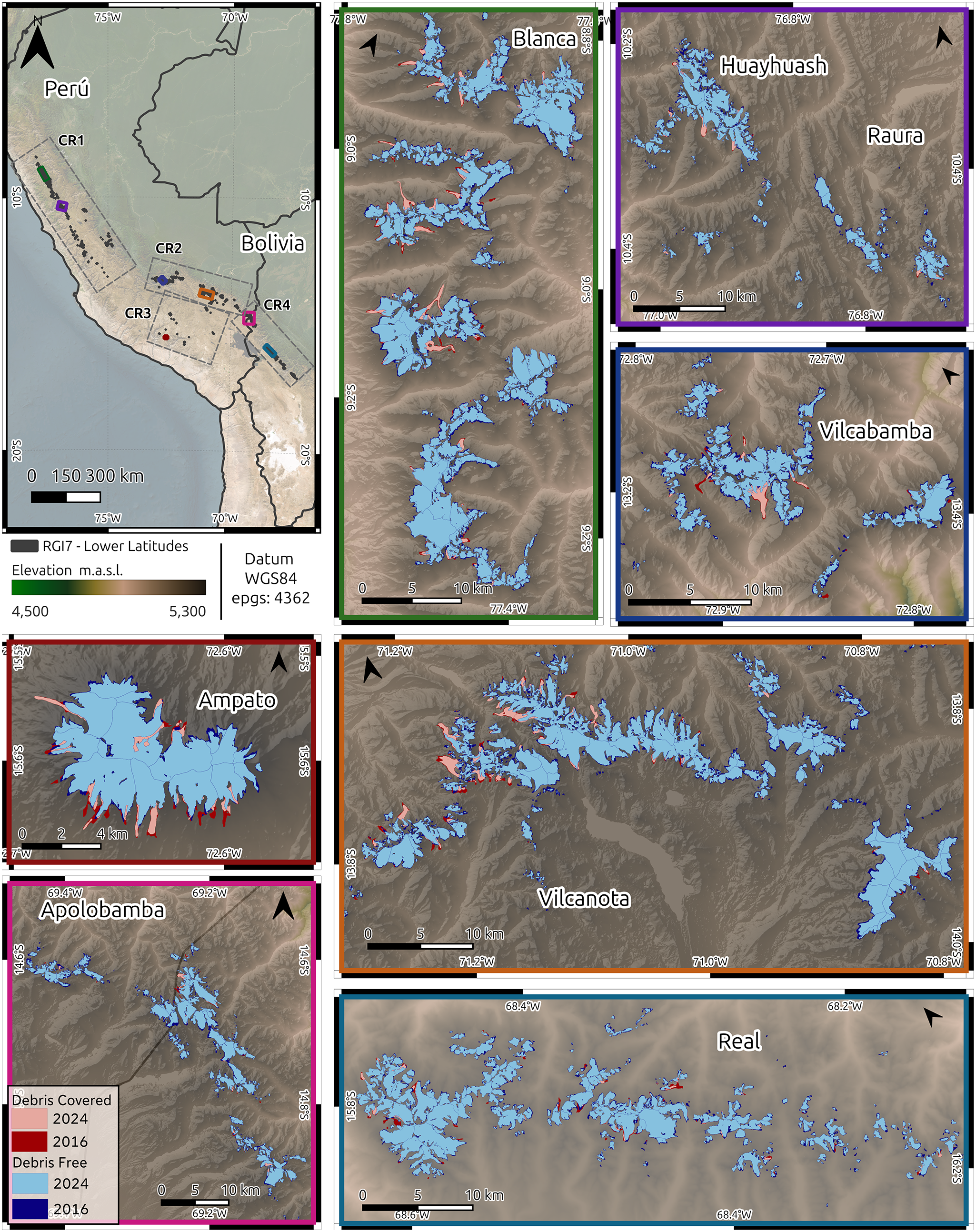
Once all the data were preprocessed, each layer was resampled via nearest-neighbor interpolation to a spatial resolution of 10 m based on the highest-resolution optical bands and merged into yearly image stacks. After this, tiles of 384x384 pixels were clipped from the stacks covering the entire glacier area, and matching the patch size required for the GlaViTU architecture. To define the sampling domain, RGI7 was used as a reference mask. Since the entire region has shown a steady glacier area decreasing trend in the last two decades (Seehaus and others, Reference Seehaus, Malz, Sommer, Lippl, Cochachin and Braun2019; Reference Seehaus, Malz, Sommer, Soruco, Rabatel and Braun2020; Malone and others, Reference Malone, Broglie and Wrightsman2022), we assumed that the glacier area did not advance further within our observation period than the areas delineated by the RGI7 (representative of the year 1998). The positions of the tiles were first determined automatically, using a regular grid generated to cover all areas intersecting the RGI7 polygons, and manually optimized to minimize the total number of tiles. These tiles overlap up to 8 pixels ( $\approx2$%) in order to minimize boundary effects at the transition between tiles and to obtain smoother glacier outlines, similar to Chu and others (Reference Chu, Yao, Duan, Chen, Li and Pang2022) approach. The resulting database of 531 tiles was split into 60% of the tiles for training, 20% for validation and 20% for testing, covering exclusively the Peruvian region of the Tropical Andes, excluding Cordillera Apolobamba. The subset splitting was performed randomly, only considering that the tiles selected for training should contain at least 5% of glacier area according to the INAIGEM inventory. This filters out tiles with negligible ice cover (e.g., vanished glaciers) and ensures a more balanced representation of the glacier class. For the Bolivian Andes (Cordilleras Apolobamba, Real and Tres Cruces), where no comparable official inventory exists, the trained model was applied only for inference. This resulted in 139 additional tiles that were incorporated to generate the glacier outlines for this region. However, due to incomplete Sentinel 1 coverage over Cordillera Apolobamba and the northern section of Cordillera Real between 2022 and 2024, we used zero values for the missing radar data. To account for this limitation and to minimize potential misclassifications, the generated outlines over these particular areas were manually inspected and edited on-screen to ensure accuracy. Datasets were normalized using maximum and minimum values per band based on the glacier climatological regions described by Sagredo and Lowell (Reference Sagredo and Lowell2012): northern wet outer tropics (CR1), southern wet outer tropics in Peru (CR2) and Bolivia (CR4) and dry outer tropics (CR3) (see Fig. 1).
Overview of the study region (top left panel), including climatic regions (dashed-line boxes) and glacier outlines predicted for 2016 and 2024 for some selected mountain ranges. Frame colors indicate the positions in the overview map. Background: Copernicus DEM and derived hillshade.

Figure 1 Long description
The image consists of multiple panels showing glacier outlines in Peru and Bolivia for the years 2016 and 2024. The top left panel is an overview map of the study region, highlighting climatic regions CR1, CR2, CR3 and CR4, with glacier outlines marked. The remaining panels show zoomed-in views of specific mountain ranges: Blanca, Huayhuash, Raura, Vilcabamba, Ampato, Apolobamba, Vilcanota and Real. Each panel includes glacier outlines for 2016 and 2024, with debris-free and debris-covered areas indicated. Debris-free areas are shown in blue and light blue for 2016 and 2024, respectively, meanwhile debris-covered areas are shown in red and pink for 2016 and 2024, respectively.
Deep learning model
The Glacier Vision Transformer-U-Net is a hybrid architecture composed of a transformer inline with a convolutional network, designed for semantic segmentation of glaciers and recently presented by Maslov and others (Reference Maslov, Persello, Schellenberger and Stein2025). The architecture is comprised of a fusion block to fuse input information into a feature space, followed by simplified building blocks from SEgmentation TRansformer (SETR) with progressive upsampling (PUP) decoder (Zheng and others, Reference Zheng2021), and finally a U-Net module with residual connections (Ronneberger and others, Reference Ronneberger, Fischer, Brox, Navab, Hornegger, Wells and Frangi2015; He and others, Reference He, Zhang, Ren and Sun2016). This particular configuration allows a model to first learn contextual information of the input data, followed by a detailed extraction provided from the convolutional network. More details of the architecture can be found in Maslov and others (Reference Maslov, Persello, Schellenberger and Stein2025). In this study, the model was adapted and trained to predict the glacier outlines for debris-free and debris-covered glacier sections separately.
Accordingly, the input data—comprising multispectral and SAR satellite data as well as topographic information—were divided into three independent subsets: training, validation and testing (described in detail in the previous subsection). The model was trained exclusively on the training dataset to optimize the model parameters. The validation dataset was used to monitor the model performance during the training process and to select the best-performing model parameters. Finally, the independent testing dataset was used to assess the performance of the model on unseen data.
Model parameters were trained using the Adam Optimizer (Kingma and Ba, Reference Kingma and Ba2017), using a focal loss function with the focal parameter ( $\gamma$) set to 3. This value was increased compared to the standard recommended value of 2 (Lin and others, Reference Lin, Goyal, Girshick, He and Dollar2020) to address a significant class imbalance of our dataset related to debris-covered glaciers, which constitute only
 $\approx$5% of the total glacier area. Additionally, a label smoothing with the smoothing parameter of 0.1 was applied (Müller and others, Reference Müller, Kornblith and Hinton2020). Learning rate is dynamically adjusted, combining a cosine warm-up (He and others, Reference He, Zhang, Zhang, Zhang, Xie and Li2018) and cosine decay strategies with manual restarts (Loshchilov and Hutter, Reference Loshchilov and Hutter2017). During the first 10 epochs, a cosine warm-up was applied with a gradual increase of the learning rate from 1
 $\times$10
 $^{-8}$ to the initial maximum value of 5
 $\times$10
 $^{-4}$. Afterward, the learning rate follows a cosine decay pattern with an initial value set to 5
 $\times$10
 $^{-4}$, with manual restarts at epochs 20, 40, 80 and 150. This strategy helps to stabilize early training by preventing sudden weight updates and local minima. To enhance the model’s generalization capabilities, on-the-fly data augmentation was applied to the training dataset. Geometric transformations, such as random horizontal and vertical flips, rotations, cropping and rescaling, were applied simultaneously to the input data and ground-truth masks. Additionally, contrast adjustments, Gaussian noise inclusion and feature occlusion were applied only to the input predictors. Model performance was assessed using the Intersection over Union (IoU) metric, selected for its robustness in quantifying the spatial overlap between the predicted and the ground-truth pixels. Additionally, the Recall metric was included to evaluate the proportion of actual glacier pixels correctly identified by the model. The F1-Score was employed to support and evaluate performance under class imbalance conditions. Parameters of the best-performing models (tested on the validation data set for each class) were saved for later analysis. Finally, the best-performing model was assessed using the independent testing dataset. All metrics used for evaluation are summarized in Table 1.
Evaluation metrics used to assess model performance.

Table 1 Long description
Three-column table presenting metrics used to evaluate model performance, their mathematical formulas and a short description. Intersection over Union (IoU) measures the spatial overlap between the predicted and actual segmentation masks. The F1-Score is the harmonic mean of precision and recall, providing a balance between the two. Recall indicates the proportion of the actual glacier area that the model correctly identifies.
TP: True Positives, FP: False Positives, FN: False Negatives.
Postprocessing
The model outputs per-class softmax probabilities, following the input dimension. These probability maps were spatially mosaicked to reconstruct the full study area. In the overlapping sections between tiles, the probabilities were averaged pixel-wise per class to ensure consistency and a smooth transition between tiles. The class predictions were then obtained by selecting the class with the highest probability pixel-wise. The resulting segmentation mosaics were converted to polygons, generating vector outlines for each glacier class across the entire study area. To separate individual glaciers within glacier complexes, we applied the ice divides from the RGI7 inventory, following the methodological recommendations of Racoviteanu and others (Reference Racoviteanu, Paul, Raup, Khalsa and Armstrong2009) and the implementation from Maslov (Reference Maslov2023). RGI7 glacier IDs were also integrated into the output inventories from our approach to facilitate comparison with RGI7 and further analysis. Polygons with areas below 0.01 km $^2$ (debris-free plus debris-covered areas) were deleted. This minimum area threshold was applied not only to maintain consistency with the RGI baseline inventory but primarily to exclude highly uncertain outlines. As pointed out by Leigh and others (Reference Leigh, Stokes, Carr, Evans, Andreassen and Evans2019), mapping errors increase on small ice bodies where the glacier area approaches the spatial resolution of the satellite imagery, making outlines below this threshold highly unreliable.
Confidence estimation
Confidence maps were generated for the glacier segmentation predictions following the methodology of Maslov and others (Reference Maslov, Persello, Schellenberger and Stein2025). The classification confidence was estimated using the maximum softmax output as confidence  $ C(x) = max (P_i(x))$ (where
 $i$ represents the class) (Maslov and others, Reference Maslov, Schellenberger, Pandit, Persello and Stein2026). Confidence values often do not align correctly with the actual accuracy of the model (Guo and others, Reference Guo, Pleiss, Sun and Weinberger2017), and therefore, a calibration process is required to provide meaningful uncertainty results. To improve reliability, the confidence values were calibrated against the empirical accuracy, using a non-parametric calibration approach, kernel ridge regression. The calibrated confidence map
 $ \hat{C}(x) $ was obtained by mapping the calibration function pixel-wise, and represents the empirical probability that the pixel classification is correct. Calibration performance was measured using the Expected Calibration Error (ECE). Details on the methodology are comprehensively described by Maslov and others (Reference Maslov, Persello, Schellenberger and Stein2025).
Finally, the glacier area uncertainty was quantified using the calibrated probabilities. Since  $ \hat{C}(x) $ represents the probability of correct classification, we used 95% confidence bands (representing the areas where the confidence drops below 0.95 or
 $\approx$ 2 standard deviations) to qualitatively assess and visualize regions where the model’s predictions are least certain. However, to align with standard glaciological practice to quantify area uncertainty (Paul and others, Reference Paul2013), we reported our final numerical uncertainties using a 68% confidence band (1 standard deviation). For temporal area changes, uncertainties were propagated independently in quadrature.
Predictors assessment
To quantify the contribution of each data source, the Permutation Features Importance (PFI) (Breiman, Reference Breiman2001) method was applied on the trained model. The technique involves randomly shuffling a specific predictor across the test dataset (breaking the dependence between the predictor and the ground-truth), and measuring the drop in the model performance. To address the correlation between predictors from the same sensor or of the same type, we applied the method by shuffling groups of predictors together instead of permuting individual bands. Specifically, we defined four predictor groups: (1) optical (6 bands), (2) topographic variables (elevation and slope), (3) SAR coherence (ascending and descending orbits) and (4) SAR backscatter (also from both orbits). Then we performed 30 independent permutations for each group of predictors and calculated the decrease in the IoU metric of the model predictions relative to the original data. To evaluate the statistical significance of these results, we first tested normality in the results distribution with the Shapiro–Wilk test (Null Hypothesis: normally distributed sample). Finally, we determined the statistical significance of the model performance decrease using either the one-sample Student’s t-test (for normally distributed samples) or the non-parametric Wilcoxon Signed-Rank Test.
Trend analysis
To assess the statistical significance of temporal changes in glacier area, the non-parametric Mann–Kendall (MK) test (Mann, Reference Mann1945; Kendall, Reference Kendall1975) was applied. Since environmental time series often exhibit serial correlation (autocorrelation), the Trend-Free Pre-Whitening (TFPW) procedure was applied prior to the MK test (Yue and Wang, Reference Yue and Wang2002), in order to eliminate its influence on the statistical test while preserving the true trend structure. The magnitude of the trend (i.e., the rate of glacier area change per year) was estimated using Sen’s Slope estimator (Sen, Reference Sen1968), which is robust against outliers. Trends were considered statistically significant at a significance level ( $\alpha$) of 0.05.
To evaluate the drivers of interannual variability, we assessed the relationship between glacier area anomalies and the Oceanic Niño Index (ONI). To align the climate signal with the annual glacier observations (acquired typically in the dry season), monthly ONI values from NOAA (Barnston and others, Reference Barnston, Chelliah and Goldenberg1997; NOAA Physical Sciences Laboratory, 2025) were aggregated into a single annual metric by calculating the mean ONI over the hydrological year (September–August) preceding each observation. Finally, we calculated the Pearson correlation coefficient (r $_{pearson}$) between the detrended glacier area series and these aggregated ONI values to quantify the influence of ENSO phases on glacier extent.
Results and discussion
Model evaluation
Overall, the trained architecture shows a good performance segmenting glaciers in the Tropical Andes. On the testing dataset,  $IoU$ and
 $F1-score$ of 0.909 and 0.953 were obtained, respectively. The model performance improves when only debris-free areas are considered (0.926 and 0.961 of
 $IuO$ and
 $F1-score$, respectively), but drops for debris-covered glacier sections (0.431 and 0.602 of
 $IuO$ and
 $F1-score$, respectively). A summary of the model evaluation metrics is provided in Table 2. The overall scores obtained by this study are comparable to the scores achieved for the original version of the GlaViTU model in the Low Latitudes region (
 $IuO$ = 0.908) (Maslov and others, Reference Maslov, Persello, Schellenberger and Stein2025), although there were some differences that are worth mentioning. First of all, the region is not exactly the same since they only included parts of the northern wet outer tropics and did not include areas where our model struggles the most (dry outer tropics), but include regions far beyond the extent of this study, like tropical glaciers in Africa and Oceania. Moreover, this study extends the previous work and offers an additional classification of debris-covered glaciers, providing a more detailed characterization of the glacier types and area distribution.
Performance evaluation metrics (IoU, F1-score, Recall) by glacier surface type and data subset.

Table 2 Long description
The table shows performance metrics, including Intersection over Union (IoU), F1-score, and Recall, for each glacier surface type across the different datasets. The table is organized into three main categories (Combined, debris-free, and debris-covered), subdivided into datasets (training, validation, and testing). Debris-free areas consistently outperform debris-covered in all metrics. Debris-free areas achieved high accuracy metrics, with scores above 0.92 for IoU and above 0.96 for both F1-score and Recall in all datasets. However, performance drops in debris-covered areas. IoU scores drop to a range of 0.34 to 0.73, and F1-scores drop to between 0.51 and 0.85, depending on the dataset.
Combined: Overall performance across all glacier pixels (Debris-Free + Debris-Covered). Train/Val/Test: Results on the Training, Validation and Testing datasets respectively. Metrics are calculated on raw model outputs before post-processing.
Following, we analyze uncertainty estimation from the calibrated 68% confidence intervals on the independent test dataset. The model estimated a total glacier area of 160.1 km $^2$ for this subset, with a 68% confidence interval ranging from 152.3 to 170.2 km
 $^2$ (or -4.9% to +6.3% relative to the predicted area). This yields a mean regional uncertainty of approximately 5.5%. Interestingly, the total area difference on this particular dataset is about 0.8% compared to the ground-truth. This discrepancy highlights the effect of spatial aggregation: while pixel-level uncertainty along glacier margins remains, local over- and under-estimations effectively cancel each other out at the regional scale.
Our 5.5% uncertainty aligns well with previous glaciological studies, which estimate a mapping uncertainty of about 5% based on the standard deviation of multiple human annotators (Paul and others, Reference Paul2013). These studies particularly highlight the severe delineation challenges associated with very small ice bodies and debris-covered glaciers (Paul and others, Reference Paul2013; Leigh and others, Reference Leigh, Stokes, Carr, Evans, Andreassen and Evans2019). However, because these small glaciers contribute minimally to the total ice coverage, their high individual errors have little impact on the aggregated scale. Consequently, despite pixel-level uncertainties along the margins, the model yields highly accurate total area estimates at the regional scale.
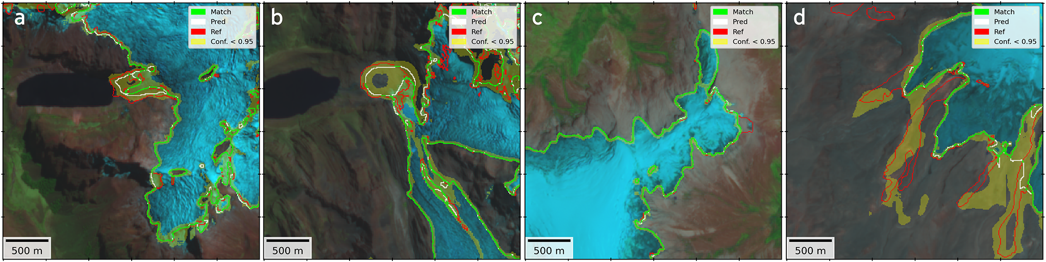
Figure 2 shows the 95% confidence bands of four tiles of the testing dataset. It can be clearly seen that debris-free glacier areas show a near-perfect match between the model and the reference inventory, as well as narrow confidence bands. An ideal example is the prediction obtained in the northern section of the Quelccaya icecap (Fig. 2c). Moreover, the model shows acceptable results for the segmentation of debris-covered sections on the glacier tongues (Fig. 2a and b), where confidence decreases notably around the margins. Although in some areas the model fails to recognize the debris-covered sections (Fig. 2d).
Segmentation results for the testing dataset, inferred using the locally trained and adapted GlaViTU model. (a) Cordillera Blanca, (b) Yerupajá glacier (Cordillera Huayhuash), (c) Quelccaya icecap north (Cordillera Vilcanota), and (d) Rumicruz glacier (Cordillera Ampatato). White lines correspond to the reference INAIGEM inventory; red lines indicate the model prediction; and green indicates areas of agreement (within  $\pm$1 pixel). Background image corresponds to a false color composition (R: B12
 $_{2.2\mu m}$, G: B8
 $_{0.8\mu m}$, B: B4
 $_{0.6\mu m}$) of the optical acquisition used for training in 2020 from the Sentinel-2 mission. Ice divides are not shown for better visualization.

Figure 2 Long description
The figure comprises four panels comparing glacier-outline predictions and reference inventory, independent of the surface type. From left to right, four different areas in the study region are shown: (a) Cordillera Blanca, (b) Yerupajáglacier (Cordillera Huayhuash), (c) Quelccaya icecap north (Cordillera Vilcanota), and (d) Rumicruz glacier (Cordillera Ampatato). In each panel white lines indicate the reference inventory, red lines show the model predictions, and green lines the areas of agreement. Yellow shaded bands around the glacier outlines show the areas where the prediction confidence drop below 95%. The background is a false-color composition from the Sentinel-2 mission on 2020, enhancing visualization of the glacier changes over time.
We observe that the model struggles under specific conditions that might influence optical imagery and SAR coherence. The model generates predictions with low confidence when a decay in reflectance in topographically shadowed areas in optical imagery is observed, even for debris-free glacier sections, e.g., as found in Yerupajá glacier (Fig. 2b). Furthermore, debris-covered glaciers are often highly heterogeneous among them, with variations in debris layer thickness and composition of the debris (Casey and Kääb, Reference Casey and Kääb2012; Rounce and others, Reference Rounce2021). Such characteristics alter optical and radar backscatter signals, which might impose additional challenges to the segmentation process. These differences due to local geology are evident when comparing our study sites. In our specific case, Rumicruz glacier (Fig. 2d) is located on the Ampato volcano, where volcanic deposits dominate (Samaniego and others, Reference Samaniego2016), whereas Yerupajá glacier (Fig. 2b) is located in the Cordillera Blanca, where batholith dominates the geology (Yonekura and others, Reference Yonekura, Matsuda, Nogami and Kaizuka1979). Consequently, debris cover at these sites will exhibit a distinctly spectral contrast for the model.
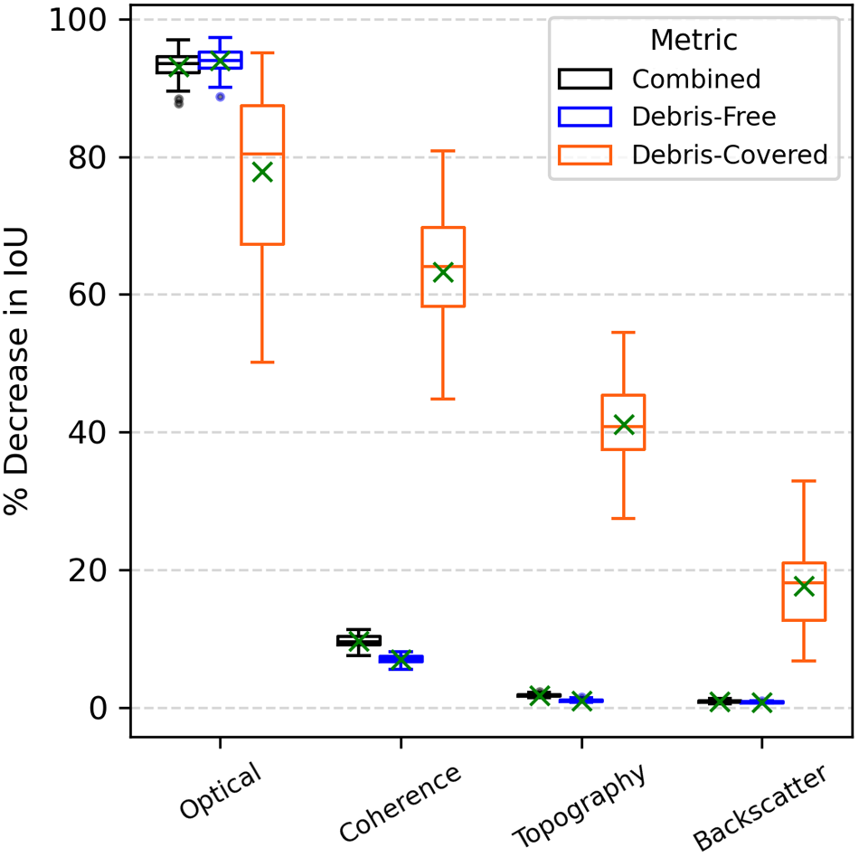
To understand the drivers of these results, we applied Permutation Feature Importance (PFI) (Fig. 3). Overall, we observed that all predictors showed a statistically significant decrease on the IoU metric (p $ \lt 0.05$) when breaking the dependence between the predictor and the ground-truth. With the exception of the debris-free DEM data, which required a non-parametric Wilcoxon signed-rank test due to non-normality, all other subsets met normality assumptions and were evaluated using a one-sample T-test. However, optical data is by far the most critical predictor overall. For both debris-free and combined metrics, shuffling optical data causes a strong decrease in performance (
 $\approx$88-97%). This indicates the model strongly relies on multi-spectral features (e.g., contrast between ice and bedrock) for the majority of the glacier area.
Boxplot of the performance decrease (IoU) from Permutation Feature Importance (PFI) analysis results, grouped by glacier surface type and combined results. The green ‘X’ marker indicates the mean value of the 30 repetitions.

Figure 3 Long description
A boxplot figure illustrating the percentage decrease in Intersection over Union (IoU) from Permutation Feature Importance (PFI) analysis across four data categories: Optical, SAR Coherence, Topography and SAR Backscatter. The metrics are represented by different colors: Combined (black), Debris-Free (blue) and Debris-Covered (orange). Each category shows varying levels of decrease, with Optical showing the highest decrease, independently of the glacier surface type. The green 'X' marks indicate the decrease of mean values of the 30 repetitions for each category.
While optical imagery is still the most important feature for debris-covered ice (IoU decrease between  $\approx$50-95%), its importance is lower and more variable than for clean ice. This variance suggests that for some debris-covered sections, optical data alone is insufficient to distinguish the glacier from the surrounding terrain. Notably, shuffling SAR coherence drops performance by
 $\approx$45-80% for debris-covered sections, suggesting that the model also strongly relies on information on surface instability and movement (decorrelation) to identify debris-covered ice. Similarly, shuffling topographic predictors causes a
 $\approx$28-55% IoU decrease, suggesting that the model likely uses slope or surface roughness to separate the glacier from stable bedrock or moraines.
In contrast, SAR coherence and topography showed a minimal impact on the model performance over debris-free glacier sections, causing only  $\approx$7% and
 $\approx$1% mean performance drops, respectively. Finally, SAR backscatter appeared to be the least critical predictor. It had almost zero impact on overall or debris-free predictions (
 $ \lt 1\%$), although it offers a moderate contribution to debris-covered detection (
 $\approx$7-32%), likely helping to detect surface texture differences.
The PFI analysis demonstrates that the model relies on optical imagery and SAR coherence to identify debris-covered sections. Consequently, inherent limitations within the SAR data are likely contributing to the underestimation of debris-covered glacier areas observed in Table 3. Since SAR coherence is the complex correlation between two acquisitions, it indicates the temporal stability of the backscatter signal, and can be used for distinguishing stable (e.g., rocks) and unstable (e.g., glaciers) surfaces (Lippl and others, Reference Lippl, Vijay and Braun2018). However, since Sentinel 1 is a side-looking instrument, imagery can be subjected to SAR layover and radar shadow, where coherence values are missing (Diaconu and others, Reference Diaconu, Heidler, Bamber and Zekollari2024). Additionally, glacier flow velocities in the Tropical Andes are often very low (typically below 50 m a $^{-1}$), reaching minimum velocities around September (Ducasse and others, Reference Ducasse, Millan, Andersen and Rabatel2024). The surface velocity might be even lower for debris-covered glacier tongues, making it difficult to observe a significant SAR coherence decorrelation over a 12-day temporal baseline. Surface velocities increase toward the wet season due to the increase in the meltwater production from September to December (Sicart and others, Reference Sicart, Hock, Ribstein, Litt and Ramirez2011; Ducasse and others, Reference Ducasse, Millan, Andersen and Rabatel2024). However, the meltwater might introduce decorrelation in the off-glacier regions, hampering the accurate mapping of the debris-covered glacier sections.
Comparison of reference (INAIGEM glacier inventory 2020) and predicted area by glacier surface type across climatic regions (CR).

Table 3 Long description
The table compares reference inventory and predicted glacier areas across three climatic regions The table is divided in three main categories (Total area, debris-free area, and debris-covered area) and subdivided in three columns each showing the reference and predicted area, as well as the difference in percentage. CR1 and CR2 show minor differences between reference and predicted total areas, while CR3 exhibits the most significant differences, with a notable decrease in both total and debris-covered areas. Overall, the total predicted glacier area is slightly less than the reference, with debris-covered areas showing the largest relative decrease. These results are based on model outputs with a minimum area threshold of 0.01 square kilometers.
Results reflect post-processed model outputs with a minimum area threshold of 0.01 km $^2$. Ref: Reference area from INAIGEM inventory. Pred: Predicted area by the model.
 $\Delta$ %: Relative percentage difference. CR1: Northern wet outer tropics. CR2: Southern wet outer tropics. CR3: Dry outer tropics.
Despite these limitations, results suggest that the model has the potential for reliable glacier segmentation in the steep mountain terrain of Tropical Andes.
To verify the final product, i.e., after post-processing, a comparison of the predicted and reference area derived from the INAIGEM glacier inventory for each climatic region for the training period (2020) is shown in Table 3. Overall, the predictions agree well with the reference data, showing a total area difference (-0.28%) well within the typical uncertainty bounds of semi-automatic outlining methodologies (Paul and others, Reference Paul2013; Leigh and others, Reference Leigh, Stokes, Carr, Evans, Andreassen and Evans2019). Specifically, the model is highly effective at segmenting debris-free sections, with minimal area differences (+0.40%). On the contrary, it underestimates debris-covered glacier areas by -12.49%, compared to the reference data. In CR1 and CR2, the total glacier area is very well reproduced, following the general pattern of overestimation of debris-free glaciers and underestimation of debris-covered glaciers. In contrast, in the smallest region, CR3, it generally underestimates the total glacier area. Although the reference inventory represents a remarkable effort and achieved outstanding evaluation metrics (INAIGEM, 2023), it is not error-free and may contain inaccuracies in challenging areas such as debris-covered sections, which could influence model training.
Glacier area changes
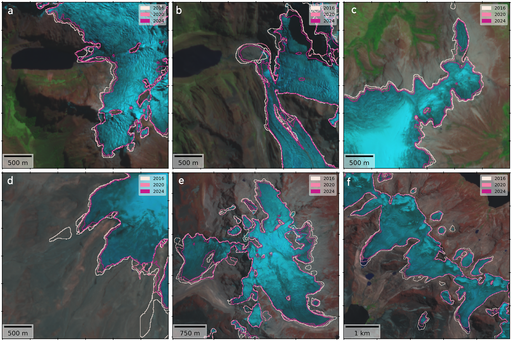
An overview of the resulting outlines for 2016 and 2024 is shown in Fig. 1, where glacier area change can be observed during this period in each of the sub-regions. A closer inspection (Fig. 4) highlights that the shrinkage is particularly enhanced in lower elevations and at the glacier tongues. In some areas, such as the Quelccaya icecap and Cordillera Tres Cruces (Fig. 4c and f, respectively), detachment of small ice bodies toward north-east is observed. Such fragmentation is a morphological consequence of the ongoing glacier melt and thinning (Seehaus and others, Reference Seehaus, Malz, Sommer, Lippl, Cochachin and Braun2019; Reference Seehaus, Malz, Sommer, Soruco, Rabatel and Braun2020). Concurrently, an increase in debris-covered sections toward higher elevations is observed (Fig. 4a, b and e).
Glacier outlines predictions for the years 2016, 2020 and 2024. (a) Cordillera Blanca, (b) Yerupajá glacier, Cordillera Huayhuash, (c) Quelccaya icecap north, Cordillera Vilcanota, (d) Rumicruz glacier, Cordillera Ampatato, (e) Cordillera Real and (f) Cordillera Tres Cruces. Background image corresponds to a false color composition (R: B12 $_{2.2\mu m}$, G: B8
 $_{0.8\mu m}$, B: B4
 $_{0.6\mu m}$) of the optical acquisitions used for prediction in 2024 from the Sentinel-2 mission. Ice divides are not shown for better visualization.

Figure 4 Long description
Six-panel figure containing six satellite images labeled a to f, each one displaying glacier outline predictions. The panels correspond to the following regions: (a) Cordillera Blanca, (b) Yerupajá glacier in Cordillera Huayhuash, (c) Quelccaya icecap in the north of the Cordillera Vilcanota, (d) Rumicruz glacier in Cordillera Ampatato, (e) Cordillera Real, and (f) Cordillera Tres Cruces. Glacier outlines for 2016, 2020 and 2024 are shown in white, light pink and magenta lines respectively. The background is a false color composition from the Sentinel-2 mission in 2024, enhancing visualization of the glacier changes over time.
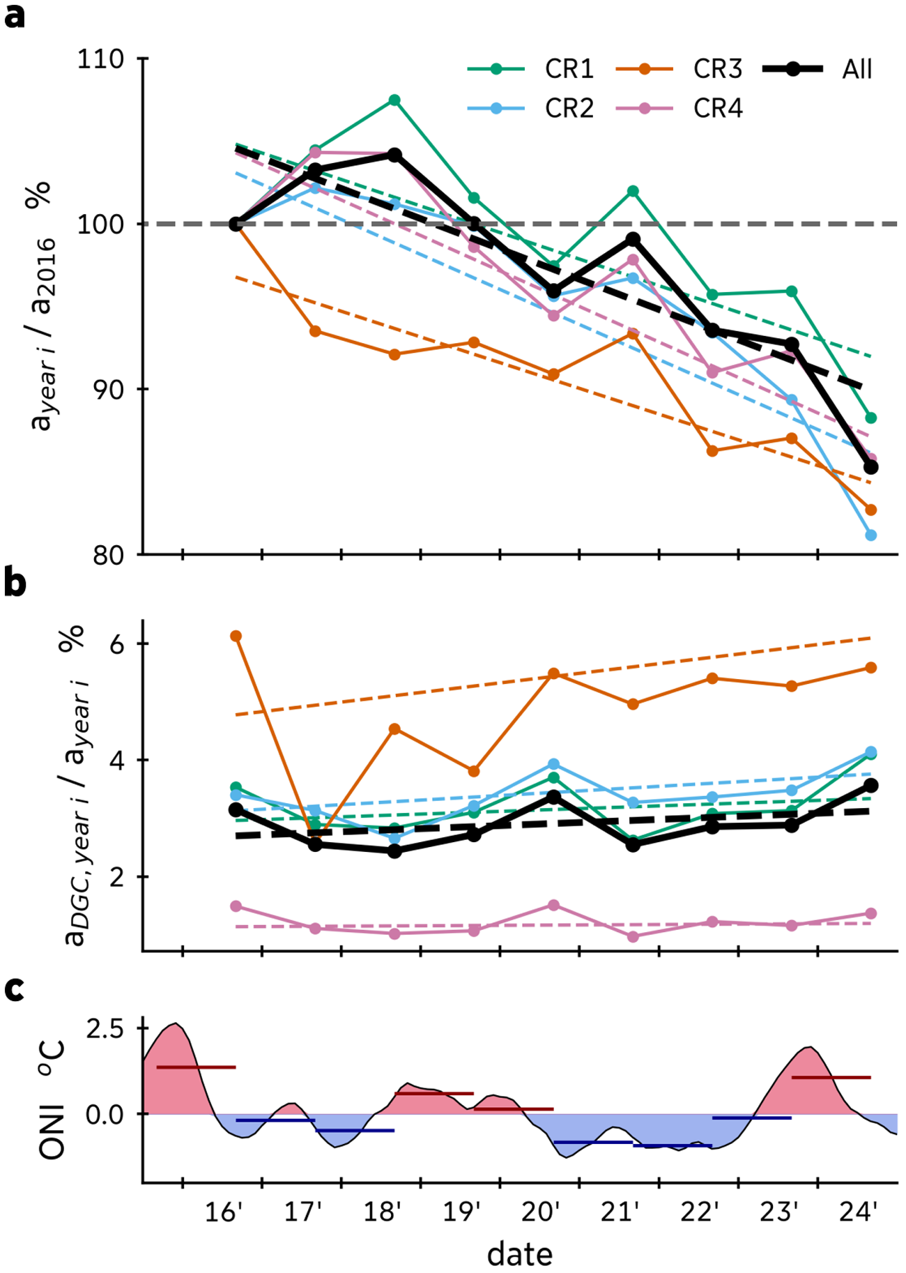
Relative to the first year of the study period (2016), an overall loss of glacier area of 201.6 $\pm$99 km
 $^2$ (
 $\approx$ 14.7%) was observed across the region by 2024 (Fig. 5a, Table 4). According to the TFPW MK test, all four regions show a consistent and statistically significant decreasing trend (
 $p$-values
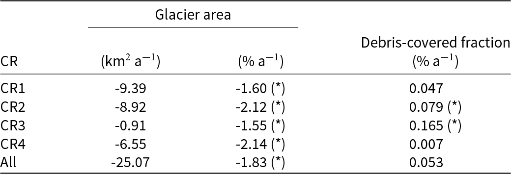
 $ \lt 0.05$) in the glacier extent (Table 5). In the case of the debris-covered area fraction (Fig. 5b), positive values of the Sen’s slope were estimated, but statistically significant trends were found only in the Peruvian southern wet outer tropics and in the dry outer tropics (CR2 and CR3, respectively). For the total glacier area, the Sen’s slope estimator indicates an area reduction of -25.07 km
 $^2$ a
 $^{-1}$, which corresponds to -1.83% a
 $^{-1}$, concentrated in the wet outer tropics (
 $\approx$ 96% of the region-wide area loss). Particularly, the southern wet outer tropics exhibit the fastest decrease, with area change rates of -2.12% a
 $^{-1}$ and -2.14% a
 $^{-1}$ in the Peruvian (CR2) and Bolivian (CR4) regions, respectively. When compared to the RGI7 inventory, the cumulative area reduction accounts for 563.8
 $\pm$108 km
 $^2$ between 1998 and 2024, which is equivalent to 32.5% of total area loss and
 $\approx$ 21.7 km
 $^2$ a
 $^{-1}$, which suggests an acceleration of glacier area decrease in the recent decade.
Temporal evolution of glacier area and climatic forcing in the Tropical Andes (2016–24). (a) Glacier area change relative to 2016. Absolute area values for each region (CR) and year are detailed in Table 4. (b) Evolution of debris-covered glacier sections relative to total glacier area. Dashed lines indicate long-term trends estimated using Sen’s slope. (c) Oceanic Niño Index (ONI), with red and blue shading indicating El Niño (warm) and La Niña (cold) phases, respectively. Colored horizontal segments denote the mean ONI value aggregated over the hydrological year (September–August) preceding each annual glacier observation.

Figure 5 Long description
The image contains three vertically stacked line plots, with a shared x-axis labeled as “date”. The first plot (a) shows glacier area change relative to 2016 glacier area in percentage. Each solid line represents CR1 (green), CR2 (cyan), CR3 (orange), CR4 (pink), and regions All (black). Dashed lines indicate the long-term trends. The second plot (b) shows the evolution of debris-covered glacier fraction relative to total glacier area, with the same color scheme. The third plot (c) shows the Oceanic Niño Index (ONI) in degrees Celsius. Fluctuations in red and blue shading indicate El Niño and La Niña phases, respectively, from 2016 to 2024. Sharp declines in the glacier area lines in plot (a) align vertically with the red-shaded El Niño (warm) phases in plot (c).
Glacier area timeseries (km $^2$) from 2016 to 2024 and from RGI7 for the four regions and the whole study area.

Table 4 Long description
The table presents glacier area measurements in square kilometers for four regions and the entire study area from 2016 to 2024, including RGI7 data as a reference point from 1998. CR1 experienced a decrease in glacier area from 585.2 in 2016 to 516.6 in 2024. CR2 also decline from 421.2 to 342.0 over the same period. CR3 decreased from 58.2 to 48.2 and CR4 from 305.0 to 261.7. The total glacier area for all regions combined decreased from 1369.7 in 2016 to 1168.1 in 2024.
The corresponding relative area changes are visualized in Figure 5a.
Trend Free Pre-Whitening Mann–Kendall (TFPW-MK) test results for normalized glacier area and debris-covered glacier fraction changes from 2016 to 2024 across four regions.

Table 5 Long description
The table presents the results of the Trend Free Pre-Whitening Mann-Kendall statistical test on glacier area and debris-covered fraction changes from 2016 to 2024 across four regions. Negative and significant trends in the glacier area are observed in all regions, with CR2 and CR4 exhibiting the fastest decrease, both above 2.1 percent per year. Debris-covered fraction shows a positive trend in all regions, but only significant in CR2 and CR3. Overall, the combined data for all regions indicates a significant decrease in glacier area of 25.07 square kilometers per year and a slight increase (non-significant) in debris-covered fraction.
Trends were estimated using Sen’s Slope estimator. (*) indicates a statistically significant trend ( $\alpha$=0.05).
Our results are in agreement with previous studies in the same region (see Table S1). The results are similar to the inventories produced by local authorities in 2016 (INAIGEM, 2018) and 2020 (INAIGEM, 2023), although our model yields slightly lower total area estimates. Compared to regional glacier mapping in Peru and Bolivia for the period 2000–16 (Seehaus and others, Reference Seehaus, Malz, Sommer, Lippl, Cochachin and Braun2019; Reference Seehaus, Malz, Sommer, Soruco, Rabatel and Braun2020), our results indicate smaller area changes and a slower reduction trend, which is most probably related to the selection of the reference year, and second, inherent differences of the remote sensing products used (e.g., spatial resolution). Since 2000 was not an El Niño year, it is likely that the mapped glacier area was overestimated by Seehaus and others (Reference Seehaus, Malz, Sommer, Lippl, Cochachin and Braun2019; Reference Seehaus, Malz, Sommer, Soruco, Rabatel and Braun2020) (see below for an analysis of the impact of ENSO on the glacier mapping). On average, their estimations for 2000 are  $\approx$27% higher than RGI7’s, and in 2016
 $\approx$14% compared to ours.
To directly compare our results with the RGI7 baseline (1998) at a glacier scale, we analyzed the long-term area evolution of two benchmark glaciers in the study region: Artesonraju and Zongo glaciers. For Artesonraju, the glacier area decreased from 5.94 $\pm$0.30 km
 $^2$ in 1998 to 5.63
 $\pm$0.31 km
 $^2$ in 2016, and further decreased to 5.29
 $\pm$0.29 km
 $^2$ by 2024, representing a total area loss of approximately 10.9% since 1998. Similarly, Zongo glacier exhibited a pronounced reduction from 2.40
 $\pm$0.12 km
 $^2$ in 1998 to 2.13
 $\pm$0.12 km
 $^2$ in 2016, and down to 1.94
 $\pm$0.12 km
 $^2$ in 2024, yielding an overall area loss of roughly 19.2% over the period 1998–2024. It is notable that the relative area decrease of these benchmark glaciers is lower than the general trend of the region. However, this can be explained by the fact that these glaciers are larger than most of the glaciers of this region. By 1998, only
 $\approx$ 13% of the glaciers had an area greater than 1 km
 $^2$. Because smaller ice bodies are significantly more susceptible to ablation (Francou and others, Reference Francou, Vuille, Wagnon, Mendoza and Sicart2003), we assume that the regional shrinking rate is higher due to the accelerated retreat of these predominant smaller glaciers (Rabatel and others, Reference Rabatel2013; Seehaus and others, Reference Seehaus, Malz, Sommer, Lippl, Cochachin and Braun2019).
Although results on debris-covered area fraction do not show a statistically significant trend (Fig. 5b) in all cases, the positive tendency aligns with the increase observed in regions such as the Himalaya (Bolch and others, Reference Bolch, Buchroithner, Pieczonka and Kunert2008; Thakuri and others, Reference Thakuri2014) or the Southern Andes (Glasser and others, Reference Glasser, Holt, Evans, Davies, Pelto and Harrison2016). Such expansion of glacier debris cover areas has been widely associated with ongoing climate warming (Herreid and Pellicciotti, Reference Herreid and Pellicciotti2020), because a debris layer on the glacier insulates the ice surface from the atmosphere and therefore delays its response to climate variability compared to clean-ice glaciers (Vincent and others, Reference Vincent2016). Moreover, the warming also destabilizes the surrounding rock-walls (often stabilized by permafrost), leading to higher deposition of debris on the glaciers (Zhong and others, Reference Zhong2022).
Glacier area fluctuated across all regions, revealing a clear inverse relationship with the debris-covered fraction (Fig. 5a and b): temporary increases in total glacier area coincided with drops in the debris-cover fraction for most of the regions. This indicates that the interannual variation is predominantly driven by expansions of the debris-free (clean ice and snow) area, rather than changes in the debris-covered sections. Furthermore, glaciers in the dry outer tropics (CR3) behave quite differently in the first half of the study period (2016–20), showing a decrease in area for 2017 and 2018, contrary to the other regions. Given the short time frame and the small glacier area, it is unlikely that small inter-annual area increases can be associated with an actual advance of the glaciers. Instead, these results might be influenced by climate anomalies from ENSO events, their impact on snow cover and the timing of acquisitions of the remote sensing data.
Correlation analysis (Fig. S1) reveals a strong negative correlation (r $_{pearson} \lt -0.72$) between the annually aggregated ONI index and the total glacier area anomalies for all regions, except CR3 (r
 $_{pearson}$ = 0.09). This means that in the years during strong El Niño events (2016, 2020 and 2024), the mapped glacier area tends to decrease, whereas during la Niña events the glacier area kept stable or even increased (Fig. 5a and c). During El Niño (warm phase) events, the outer tropics region experiences increased air temperatures and reduced precipitation (Garreaud, Reference Garreaud2009). These conditions lead to less snow accumulation, resulting in a longer ice surface exposure and therefore a low albedo over the glacier surface due to the lack of fresh snow cover (Maussion and others, Reference Maussion, Gurgiser, Großhauser, Kaser and Marzeion2015). Consequently, the absorption of shortwave radiation is enhanced and melting is accelerated. Furthermore, due to clear sky conditions, both incoming shortwave and longwave radiation are higher (Francou and others, Reference Francou, Vuille, Wagnon, Mendoza and Sicart2003). On the contrary La Niña (cold phase) events often bring cooler temperatures and enhanced precipitation in the outer tropics (Garreaud, Reference Garreaud2009), which promote a higher surface albedo due to fresh snow accumulation, and increased cloud cover, all of which act to reduce net radiation and melting rates (Francou and others, Reference Francou, Vuille, Wagnon, Mendoza and Sicart2003). Glaciers respond accordingly, showing more negative glacier mass balance during El Niño events, whereas neutral or slightly positive glacier mass balances are exhibited during La Niña events (Vuille and others, Reference Vuille, Kaser and Juen2008). Therefore, glacier mapping is most probably influenced by persistent snow patches remaining from the wet season due to climate anomalies from ENSO events (see example in Supplementary Fig. S2), which is consistent with Malone and others (Reference Malone, Broglie and Wrightsman2022) findings. Despite the interannual fluctuations, long-term trends of glacier loss agree with the observations by others (e.g., increased ELA trends, glacier thinning) (Vuille and others, Reference Vuille2018).
An important source of uncertainty is the sensitivity of the glacier area mapping process to the timing of satellite imagery acquisition. Depending on weather conditions, the glacier extents mapped by this method can change significantly over short time scales, since it relies partly on surface reflectances and conditions (Malone and others, Reference Malone, Broglie and Wrightsman2022; Huang and Kinouchi, Reference Huang and Kinouchi2024). In the Tropical and Subtropical Andes, accumulation and ablation do not follow the distinct seasonal patterns seen in mid-latitudes (Veettil and others, Reference Veettil, Wang, Florêncio De Souza, Bremer and Simões2017). Instead, these processes often occur simultaneously, driven by regional precipitation patterns and temperature fluctuations rather than a clear distinction between summer and winter cycles (Veettil and others, Reference Veettil, Wang, Florêncio De Souza, Bremer and Simões2017). As a result, acquisitions from different times of the year, or even within the same season, might capture variable temporal snow cover. This variability can affect how glacier boundaries are mapped, potentially leading to overestimation of glacier extents. Within this study, we tried to minimize seasonal biases by selecting imagery for each year from the same season. However, cloud-cover or imagery availability forced us partly to include also images from extended time windows.
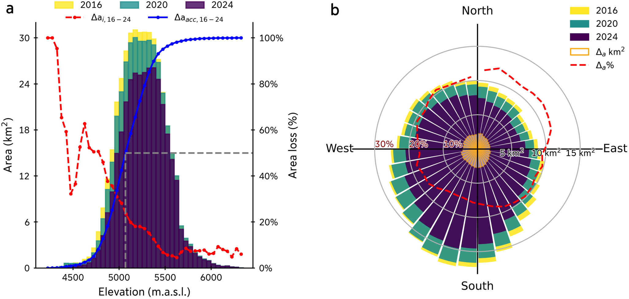
Figure 6a and b shows the area distribution and area loss depending on the elevation and aspect for glaciers located in the Peruvian southern wet outer tropic. The results of the remaining regions can be found in Fig. S3–S8 (Supplementary Information). To minimize the impact of persistent snow patches, we only analyzed outlines from years after strong El Niño events, which are 2016, 2020 and 2024.
In general, the greater area change rates are concentrated in lower elevations of the glaciers, but the absolute area loss is concentrated at mid elevations and is generally pronounced at glaciers with south-west orientations, which is dominating the glacier orientation. When analyzing the median elevation of area loss—the elevation at which 50% of the glacier area loss occurred between 2016 and 2024—distinct regional differences are observed. In the northern wet outer tropics, the median elevation of area loss is located at  $\approx$ 4973 m a.s.l., while in the southern wet outer tropics of Peru, it rises up to
 $\approx$5070 m a.s.l., and increases even more for Bolivian glaciers up to
 $\approx$5187 m.a.s.l. In the dry outer tropics (CR3), it reaches
 $\approx$5550 m a.s.l., indicating that glacier area change is concentrated at significantly higher elevations, which corresponds to the generally higher location of the median glacier elevations, with a predominant area decrease toward south to south-west-facing slopes. Across all regions, glacier area is predominantly decreasing on slopes facing between south and west, with a slight shift toward south-to-southeast-facing slopes in CR4.
Glacier area distribution and changes in region CR2, Peruvian southern wet outer tropics, for the years 2016, 2020 and 2024. (a) Hypsometric profile of glacier area across elevation bands (colored bars, left axis). The blue line indicates the accumulated area loss, while the red line shows the bin-relative area loss (right axis). The dashed gray line marks the median elevation of area loss, elevation below which 50% of the cumulative area loss occurred. (b) Polar plot of glacier area by aspect. Colored bars show the area per directional sector, with white-orange bars highlighting the absolute area loss between 2016 and 2024. The dashed red line illustrates the relative area loss per aspect bin.

Figure 6 Long description
The figure image shows two plots. The first (a) is a hypsometric profile showing glacier area across elevation bands. The left axis represents area in square kilometers with colored bars representing the years 2016 (yellow), 2020 (green) and 2024 (purple). The right axis shows the area loss in percentage, with a blue line indicating accumulated area loss and a red line showing bin-relative area loss. A dashed gray line marks the median elevation of area loss. The second graph (b) is a polar plot of glacier area by aspect. Colored bars show the area in square kilometers per aspect bin for the years 2016, 2020 and 2024 with the same color scheme. Additional white-orange bars highlight the absolute area loss per aspect bin between 2016 and 2024 in square kilometers, and a dashed red line illustrates the relative area loss per aspect bin percentage.
It is interesting to note that although west-to-south orientations account for the greatest absolute glacier area loss, normalizing these values reveals the underlying topoclimatic signal. Specifically, in the wet outer tropics (CR1, CR2 and CR4), the relative area loss is higher over east to north-east facing slopes. This topoclimatic vulnerability aligns with findings of studies in Cordillera Blanca (Veettil, Reference Veettil2018) and Vilcanota (Veettil and De Souza, Reference Veettil and De Souza2017), and mass balance studies in Peru (Seehaus and others, Reference Seehaus, Malz, Sommer, Lippl, Cochachin and Braun2019), and Cordillera Real, Bolivia (Soruco and others, Reference Soruco, Vincent, Francou and Gonzalez2009).
South-to-west-facing areas account for the majority of the small glaciers at low altitudes (Seehaus and others, Reference Seehaus, Malz, Sommer, Lippl, Cochachin and Braun2019) and therefore are more affected by the increasing trends of surface air temperature within the last century (Vuille and others, Reference Vuille, Kaser and Juen2008). In the case of east to north-east facing slopes, they have a longer exposure to shortwave radiation throughout the year (Soruco and others, Reference Soruco, Vincent, Francou and Gonzalez2009; Veettil, Reference Veettil2018). Furthermore, they are sensitive to changes in moisture transport from the Amazon rainforest. Particularly during warm phases of ENSO, when moisture is blocked by stronger westerly winds, it causes drought conditions, especially in the southern wet tropics (Vuille, Reference Vuille2013). On top of this, once glaciers reach a certain critical size, boundary effects such as heat flux and long-wave radiation emitted by the surrounding hot rocks can no longer be neglected, triggering an accelerated decrease (Francou and others, Reference Francou, Vuille, Wagnon, Mendoza and Sicart2003). Moreover, with an Equilibrium Line Altitude above the upper glacier reaches, the absence of a permanent accumulation area dampens the mass transfer toward lower elevations and further leads to frontal recession, as documented in Chacaltaya, Charquini (Bolivia), Yanamarey (Peru), La Conejeras (Colombia) glaciers (Francou and others, Reference Francou, Vuille, Wagnon, Mendoza and Sicart2003; Rabatel and others, Reference Rabatel2013).
Critical shrinkage and loss of small glaciers
Compared to the RGI7 inventory baseline, we estimate that 1261 glaciers vanished or shrank below the 0.01 km $^2$ mapping threshold by 2024. When strictly analyzing years after strong El Niño events (2016, 2020 and 2024) to minimize snow cover artifacts, we found that 825 glaciers shrank below the area threshold by 2016, and an additional 436 glaciers dropped below the detection limit between 2016 and 2024. Because of the 10 m spatial resolution of the remote sensing data, it is not possible to state without a high uncertainty whether these extremely small ice bodies have completely disappeared or remain as small ice fragments (Leigh and others, Reference Leigh, Stokes, Carr, Evans, Andreassen and Evans2019).
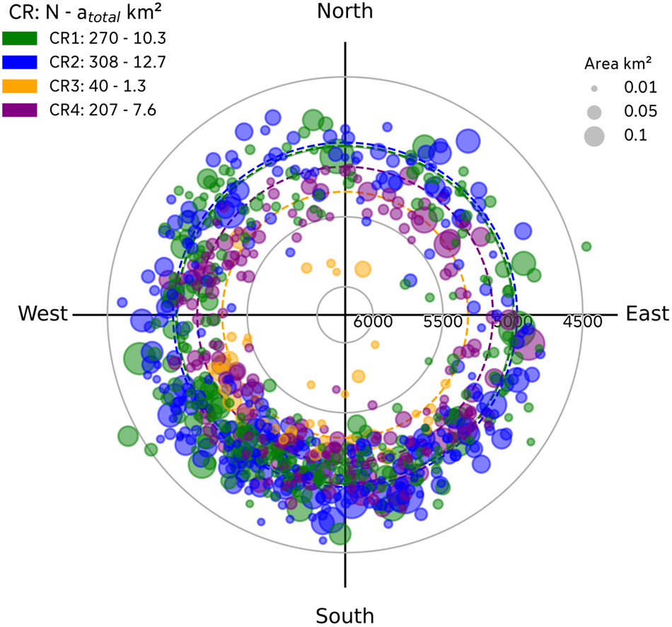
Figure 7 and S9 summarize the topographic characteristics of glaciers that shrank below the threshold between 1998 and 2016, and between 2016 and 2024, respectively. A regional overview of these glaciers can be found in Fig. S10.
All glaciers that dropped below the threshold during the first period (1998–2016) were relatively small glaciers in 1998 according to RGI7, with a mean area of 0.039 km $^2$, and 75% with areas smaller than 0.044 km
 $^2$. The maximum glacier size in this group was only 0.31 km
 $^2$, and in total, they accounted for 1.8% of the ice area in 1998. In the subsequent period (2016–24) glaciers that shrank below the mapping threshold had a mean area of just 0.028 km
 $^2$ (75% with areas smaller than 0.031 km
 $^2$) and a maximum size of 0.23 km
 $^2$. Although these glaciers were substantially larger in 1998 (mean area of 0.083 km
 $^2$), their recent shrinking below the detection limit underscores a progressive ice loss rather than an abrupt area reduction. Most of these glaciers in both periods exhibited a south-west to south-facing orientation, except for the Bolivian wet outer tropics, which exhibit a peak toward south-east orientations.
Topographic characteristics of glaciers that had shrunk below 0.01 km $^2$ between 1998 and 2016 according to the RGI7 inventory, shown for each climatological region. Each marker represents a glacier, plotted by its mean elevation (radial distance) and aspect (angular direction). Dashed circle lines represent the area-weighted mean elevation for each region.

Figure 7 Long description
A polar plot displays glacier data with markers representing individual glaciers that had shrunk below 0.01 square kilometers between 1998 and 2016. The radial distance indicates mean elevation, the angular direction shows aspect, and the marker size the glacier area in 1998. Different colors represent climatological regions: CR1 (green), CR2 (blue), CR3 (orange), and CR4 (purple).
Notably, the results show a certain regional variability in terms of elevation (Fig. 7). The regional distribution shows that the Peruvian wet outer tropics (CR1 and CR2) hosted the greatest number of glaciers with areas below the detection limit (270 and 308, respectively), both with mean elevations slightly below 5000 m a.s.l. Toward the south in the Bolivian wet outer tropics, the mean elevation of these glaciers increased up to 5142 m a.s.l. In contrast, in the dry outer tropics, CR3, the recorded amount of glaciers that shrank below 0.01 km $^2$ is smaller, but the mean elevation is significantly higher compared to the other regions (5320 m a.s.l.), which corresponds to both the low total glacier coverage and the generally higher average glacier elevations. In our study period, we observed that the orientation distribution of these glaciers remained similar to that observed for the 1998–2016 period, but presents higher mean elevations, especially for region CR3. It is worth noting that CR3 contains several glaciers on volcanoes and a relatively high number of debris-covered glaciers, which are especially challenging for our model to delineate accurately.
Overall, these findings emphasize that small glaciers below 0.05 km $^2$ are particularly vulnerable to shrinking below the 0.01 km
 $^2$ threshold. The strong spatial and topographic patterns identified here—namely, the heightened vulnerability of south-west facing glaciers and the distinct regional elevation thresholds for glacier survival (e.g.,
 $ \lt 5000$ m a.s.l. in the Peruvian wet tropics versus
 $ \lt 5320$ m a.s.l. in the dry outer tropics)—support the idea that regional-scale climatic drivers, amplified by size and elevation constraints, play a dominant role in controlling glacier persistence in the Tropical Andes.
Although these numbers may appear alarming, they are comparable to previous studies. Seehaus and others (Reference Seehaus, Malz, Sommer, Lippl, Cochachin and Braun2019) found only 177 vanished glaciers in the Peruvian Andes and the complete Cordillera Apolobamba in a similar time frame (2000–16), but this number ascends to 296 if we apply an area threshold of 0.01 km $^2$. In our study, the same region contains a total of 643 glaciers that were not detected or shrank below this threshold. We attribute the offset to the different baseline inventories, as well as to the different approaches to defining the ice divides and glacier catchments.
A notable case is Chacaltaya Glacier, a well-known vanished glacier. There, the world’s highest ski resort was located, which extended from approximately 5360 to 5140 m a.s.l. Between 1940 and 1993, the glacier exhibited a slow but steady decrease (1.1 % a $^{-1}$), but during the 1990s, when it reached an area
 $\approx$0.1 km
 $^2$, the area change ratio increased drastically (8.0% a
 $^{-1}$, between 1993 and 1998) (Francou and others, Reference Francou, Ramirez, Cáceres and Mendoza2000). In 1998, this south-facing glacier covered an approximate area of 0.06 km
 $^2$, and by then, researchers had predicted the glacier would disappear in 10 to 15 years if the climatic conditions continued (Ramírez and others, Reference Ramírez2001). Only 11 years later, the glacier had completely vanished (Liu and others, Reference Liu, Kinouchi and Ledezma2013). Interestingly, our model still detected glacier-like features on Chacaltaya glacier location after cold phases of ENSO, even though it is well known that it had vanished about 7 years before our study period. However, for the El Niño years 2016, 2020 and 2024, it correctly predicted its absence. We attribute these sporadic detections to remaining snow patches, which tend to be more persistent in high-altitude regions like Chacaltaya. This underscores the importance of performing glacier mapping after warm ENSO phases, when seasonal snow cover is minimal and true glacier extents can be more reliably delineated.
Conclusions
In this study, we present a new dataset of yearly glacier outlines (2016–24) for the Peruvian and Bolivian Tropical Andes, generated using an extended version of the GlaViTU deep learning model, to segment debris-free and debris-covered glacier areas as individual classes. The architecture demonstrated a good performance ( $IoU \gt 0.90$ and
 $F1 \gt 0.95$) on the test dataset, consistent with state-of-the-art scores for tropical glaciers. Meanwhile, accuracy is high for debris-free glaciers, but falls sharply for debris-covered tongues. Confidence-band maps show that most errors are concentrated around shadowed areas and debris-covered sections. Future applications could benefit from using different input data to improve the segmentation on debris-covered ice, such as thermal data, velocity and/or a high-resolution DEM, which target specific characteristics of debris-covered glaciers (surface temperature, motion and roughness).
Our analysis suggests that an overall loss of glacier area of 201.6 $\pm$99 km
 $^2$ (14.7%) between 2016 and 2024, with statistically significant negative trends in each sub-region. On average, 1.83% a
 $^{-1}$ of glacier area was lost, with the southern wet outer tropics shrinking fastest
 $\approx$2.1% a
 $^{-1}$. Compared to the RGI7 inventory, a cumulative area reduction of 563.8
 $\pm$108 km
 $^2$, which is equivalent to a 32.5% of glacier loss, is found for the period 1998–2024. While absolute area losses are concentrated at lower elevations and on predominantly south- to west-facing slopes, normalizing these values reveals that east- to north-east-facing glaciers exhibit the highest relative glacier area reduction.
Area timeseries show prominent fluctuations that align with ENSO interannual influences: strong El Niño years (2016, 2020, 2024) are followed by sharp declines, whereas La Niña cold phases produce stabilization or area increase, which can often be attributed to falsely mapped persistent snow patches as glaciers. We emphasize that for an optimal mapping of glacier area, it should be performed after El Niño years. This approach minimizes overestimation of glacier area due to remaining snow patches and yields the most reliable glacier inventories, which is particularly important for small glaciers near their extinction threshold.
Our study shows that  $\approx$ 1261 glaciers shrank below the 0.01 km
 $^2$ threshold and potentially disappeared, including 825 before 2016, and 436 since 2016. They are generally small (
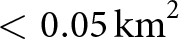 $ \lt 0.05\,\mathrm{km}^2$) and most of them are located at low elevation (
 $ \lt 5400$ m a.s.l.); 95% of those lost between 1998 and 2016 lay below 5350 m a.s.l. The combined effects of small initial size, low elevation and ENSO-driven climatic variability play an essential role in glacier persistence in the region. As glaciers shrink to these extremely small sizes, they become highly susceptible to rapid disappearance in the following years due to accelerating local feedback mechanisms.
Our analysis complements global and local glacier inventories, filling spatio-temporal gaps in the study region, one of the most vulnerable glacier regions in the world. As glacier basins become increasingly stressed under warming scenarios, glacier monitoring and particularly mapping, become fundamental for managing future water availability. The processed glacier outlines are publicly available, so they can be used by the community for various further studies as a baseline for glacier, hydrological and mass balance models. This is particularly needed in the study region, where glaciers strongly affect the mountain hydrology, and therefore water supply and socio-economic activities, but also communities whose cultural beliefs are attached to the mountains.
Supplementary material
The supplementary material for this article can be found at https://doi.org/10.1017/aog.2026.10053.
Data availability statement
The generated glacier outlines are publicly available via Zenodo. DOI: 10.5281/zenodo.19735162.
Acknowledgements
The authors would like to thank the Copernicus Programme of the European Union for providing satellite data free of charge. Moreover, we highly appreciate the public provision of the GlaViTU model by the developers (https://github.com/konstantin-a-maslov/scalable_glacier_mapping), as well as the Randolph-Glacier-Inventory Consortium and INAIGEM for providing the RGI7 global glacier inventory and the Peruvian glacier inventory, respectively. This research was supported by the Elitenetzwerk Bayern (grant no. IDP M3OCCA) and the Deutsche Forschungsgemeinschaft within the Emmy-Noether-Program (grant no. DFG SE3091/3-1). Computing infrastructure was provided via the project EVERLASTING funded by Bundesamt für Naturschutz (BfN), grant number 3523820100. We acknowledge financial support by Deutsche Forschungsgemeinschaft and Friedrich-Alexander-Universität Erlangen-Nürnberg within the funding programme ‘Open Access Publication Funding’.
In order to improve the legibility of the manuscript, the authors have used ChatGPT (https://chatgpt.com/) to look for alternative phrases. The output of this service was reviewed and edited by the authors as needed. The authors take full responsibility for the content of the presented manuscript.













 Open access

