



1. Introduction
An airfoil encountering unsteady flow has always been an essential aerodynamic issue because of its universalities in engineering practice, such as an aircraft entering fluctuating atmospheric conditions, rotating blades on rotorcraft and wind turbines, and buildings hit by wind gusts (Wang et al. Reference Wang, Hashmi, Sun, Guo, Vita, Yang and Hemida2021b; He & Xia Reference He and Xia2023). The unsteady load resulting from unsteady flow, also known as gusts, could cause wing flutter, reduction in blade lifetime (Spinato et al. Reference Spinato, Tavner, van Bussel and Koutoulakos2009) and even bridge destruction (Billah & Scanlan Reference Billah and Scanlan1991). Thus, it is critical to estimate the unsteady load and understand the effect of gusts on structures for engineers when designing aerodynamic components.
Since the early half of the 20th century, theories for unsteady load prediction of airfoils have been proposed by several scholars. Theodorsen (Reference Theodorsen1935) developed a general analytical solution for an airfoil oscillating in a steady free stream. Sears (Reference Sears1941) derived an analytical solution for the unsteady lift of airfoils encountering a sinusoidal vertical gust. Theodorsen's and Sears’ works are landmarks and are the groundwork of many unsteady load prediction theories. In their theoretical models, the airfoil is simplified to a thin plate, and a series of point vortices are distributed along with the plate and its planar wake. Unlike the quasi-steady theory (Leishman Reference Leishman2006), the solution of point vortices on the plate considers the influence of point vortices in the wake region. Sears’ theory was later extended by Goldstein & Atassi (Reference Goldstein and Atassi1976) to a second-order model to account for the effect of distortion of gust field around the airfoil. Atassi (Reference Atassi1984) concluded that despite the nonlinear dependence of the unsteady flow on the mean potential flow of the airfoil, the unsteady lift caused by the gust could be constructed by linear superposition of the Sears lift and three independent components accounting separately for the effects of airfoil thickness, airfoil camber and mean angle of attack, and derived the specific lift formulae with airfoil thickness ignored. Isaacs (Reference Isaacs1945) considered the effect of longitudinal fluctuating flow on an airfoil and provided a complete solution for a stationary airfoil encountering longitudinal gusts. As an extension of Theodorsen's work, Greenberg (Reference Greenberg1947) obtained the lift on oscillating airfoils in a sinusoidal longitudinal gust. Since it added the assumption of sinusoidal wake vorticity behind an airfoil, Greenberg's solution is more concise than Isaacs'. Van der Wall & Leishman (Reference van der Wall and Leishman1994) compared the two theories and found that the lift coefficients obtained by the two theories are similar at small amplitudes. However, a significant deviation occurs when the free flow oscillation amplitude exceeds 40 % of the mean velocity.
The classical theories have been developed for decades, but many of these theories have not been fully validated by experiments. Perhaps due to the limitations of experimental conditions, early attempts to verify the Sears theory all ended in failure (Hakkinen & Richardson Reference Hakkinen and Richardson1957; Commerford & Carta Reference Commerford and Carta1974). Jancauskas & Melbourne (Reference Jancauskas and Melbourne1986) used two airfoils with controllable circulation to generate sinusoidal vertical gusts and found that the experimental data was in good agreement with Sears’ prediction. Cordes et al. (Reference Cordes, Kampers, Meissner, Tropea, Peinke and Hölling2017) measured the Clark-Y airfoil's response to a sinusoidal vertical gust generated by active grids in a wind tunnel. They found that the experimental measurements were generally opposite to theoretical values obtained by the Sears function but were in excellent agreement with Atassi's theory. The observed discrepancy was later clarified by Wei et al. (Reference Wei, Kissing, Wester, Wegt, Schiffmann, Jakirlic, Hölling, Peinke and Tropea2019). They analysed Sears’ theory and Atassi's theory and found that for a symmetric zero angle of attack airfoil, the two theories can achieve equivalence with an appropriate normalisation method, which was further confirmed by their experimental data. In addition, their results confirmed the validity of both theories for a NACA0006 airfoil with a zero angle of attack. Young & Smyth (Reference Young and Smyth2021) selected an airfoil with a thickness of 21 % chord and camber of 2 % chord for testing. The results suggested that the Atassi function can predict the unsteady lift experienced by airfoils for vertical gusts with a longitudinal oscillating component under small gust amplitude. When the gust amplitude was slightly larger, a significant deviation was observed. They believed that this was because Atassi's lift formula did not consider the influence of the airfoil thickness, and the thicker airfoil used in the experiment might cause deviation.
Verification of Greenberg's theory has only begun in recent years. Granlund et al. (Reference Granlund, Monnier, Ol and Williams2014) experimentally investigated the unsteady lift of a NACA 0009 airfoil under a sinusoidal longitudinal gust with a dimensionless gust amplitude of σ = 0.1, which is defined as the ratio of the longitudinal-gust amplitude to free-stream velocity. Their results showed that Greenberg's theory agreed well with measured lift history when the attack angle was below the airfoil's static stall angle, regardless of gust frequency. For larger angles of attack, there was a marked departure between the measured lift history and that predicted from Greenberg's formula. Comparable results were also found in the numerical study by Choi, Colonius & Williams (Reference Choi, Colonius and Williams2015). However, Yang et al. (Reference Yang, Li, Ma and Li2017) found considerable discrepancies between experimental results and Greenberg's prediction even under attached flow conditions. It should be noted that they experimentally chose a dimensionless gust amplitude of σ = 0.2, which is larger than that selected by Granlund et al. (Reference Granlund, Monnier, Ol and Williams2014). Recently, Ma et al. (Reference Ma, Yang, Li and Li2021) assessed the applicability of Greenberg's theory to airfoils undergoing pitching motion and encountering longitudinal gusts. They found that the experimental results generally agreed well with the theoretical prediction, which instilled considerable confidence in the validity of Greenberg's theory. Strangfeld et al. (Reference Strangfeld, Müller-Vahl, Nayeri, Paschereit and Greenblatt2016) studied a two-dimensional airfoil encountering large-amplitude harmonic oscillatory flow (σ ≈ 0.5). They found that Isaacs' theory was more precise than Greenberg's theory at a larger gust amplitude, which confirms the statement of van der Wall & Leishman (Reference van der Wall and Leishman1994) that Greenberg's theory is not accurate when the longitudinal-gust amplitude is higher than 40 % of the mean velocity. The viscous effect reduces at a high Reynolds number, which is considered closer to the assumptions of Isaacs' theory. Therefore, Zhu et al. (Reference Zhu, Mccrink, Bons and Gregory2020) conducted an experimental study to verify the Isaacs theory at a Reynolds number of 106. Nevertheless, more significant deviations from the theoretical results were observed. By measuring the time-resolved background-oriented schlieren displacement field, they found that the trailing-edge stagnation streakline violated the classical Kutta condition under the unsteady flow. It reveals that a higher Reynolds number conforms to the inviscid hypothesis but leads to other deviations.
It can be seen from the literature review that the experimental verification of the theory is preliminary, and more experimental data are still needed to examine these theories. Many recent studies focusing on mitigating gust-induced loads draw upon the foundation of classical potential flow theory (Andreu-Angulo & Babinsky Reference Andreu-Angulo and Babinsky2022; Sedky et al. Reference Sedky, Gementzopoulos, Andreu-Angulo, Lagor and Jones2022), which accentuates the significance of conducting theoretical validation. For Atassi's theory, whether thinner airfoils are more in line with the prediction result remains uncertain. For Greenberg's theory, the influence of small longitudinal-gust amplitudes on the predictive accuracy of theory has not yet been investigated. Furthermore, at low Reynolds numbers, a nonlinear relationship between the lift coefficient and angle of attack emerges, even in cases involving steady flow. This phenomenon arises from the existence of laminar separation bubbles and flow separation. It prompts contemplation about whether an amended theory grounded in steady-state outcomes can extend the theory's range of applicability. The data in this study give new information to answer these questions. The present investigation focuses on the aerodynamic response of an airfoil in vertical and longitudinal gusts. The objective is to explore the scope of applicability of these theories. Furthermore, theoretical corrections were incorporated to broaden the applicability of the theory. Flow field measurements were carried out to reveal the flow mechanism of the airfoil's response to gust-induced perturbations.
2. Theoretical model
2.1. Inflow condition
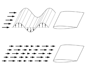
Sears’ theory is used to find the unsteady lift of an airfoil encountering sinusoidal vertical gusts, as shown in figure 1. In Sears’ model, the longitudinal component of free-stream velocity U remains constant and the vertical component v periodically propagates downstream. Vector forms of free-stream velocity can be expressed as
 \begin{equation}\boldsymbol{u} = U\boldsymbol{i} + \hat{v}\!\exp\!\left[ {{\rm i}\!\left( {\frac{{2x}}{c}{k_1} - \frac{{2U}}{c}{k_1}t} \right)} \right]\boldsymbol{j},\end{equation}
where  $\hat{v}$ is the amplitude of the vertical velocity fluctuations, k 1 is the reduced frequency associated with gusts travelling longitudinally, c is the airfoil chord length and i and j are longitudinal and vertical unit vectors, respectively.
Schematic diagram of vertical gusts.

As an extension of Sears’ theory, Atassi's theory considers the extra longitudinal velocity perturbations. Incoming flow velocity can be expressed as
 \begin{equation}\boldsymbol{u} = U\boldsymbol{i} + (\hat{u}\boldsymbol{i} + \hat{v}\boldsymbol{j})\!\exp\!\left[ {{\rm i}\!\left( {\frac{{2x}}{c}{k_1} + \frac{{2y}}{c}{k_2} - \frac{{2U}}{c}{k_1}t} \right)} \right],\end{equation}
where  $\hat{u}$ is the amplitude of the longitudinal velocity fluctuations and k 2 is the reduced frequency associated with gusts travelling vertically. Atassi (Reference Atassi1984) gave
 $\hat{u}$ and
 $\hat{v}$ as follows:
 \begin{equation}\hat{u}\boldsymbol{i} + \hat{v}\boldsymbol{j} = \varepsilon U\left( { - \frac{{{k_2}}}{{|{k_1} + {\rm i}{k_2}|}}\boldsymbol{i} + \frac{{{k_1}}}{{|{k_1} + {\rm i}{k_2}|}}\,\boldsymbol{j}} \right),\end{equation}
where  $\varepsilon$ is gust strength.
When k 2 = 0, (2.2) collapses into (2.1), i.e. Sears’ problem is a particular case of the Atassi problem. In (2.2), incoming flow velocity u is a function of x and y, indicating that perturbations propagate in both the x and y directions. The propagation direction of the perturbation is expressed as
 \begin{equation}\boldsymbol{l} = {k_1}\boldsymbol{i} + {k_2}\,\boldsymbol{j}.\end{equation}
Since the vectors in (2.3) and (2.4) are orthogonal, the incoming flow fluctuation direction and propagation direction are always perpendicular, which is a distinguishing feature of the Sears and Atassi gust types.
The gust type described by Greenberg is shown in figure 2, where the free-stream velocity only has fluctuations in the longitudinal direction. The incoming flow velocity can be decomposed into the steady-state component and fluctuation component, and variation follows
 \begin{equation}u = U + u^{\prime} = U + \sigma U{\textrm{e}^{\textrm{i}2{\rm \pi} ft}},\end{equation}
where U represents the constant free-stream velocity,  $u^{\prime}$ is longitudinal velocity fluctuation, and f is the frequency of the oscillating free stream. It can be noticed from (2.5) that the incoming flow velocity described by Greenberg vary only with time and remains independent of the streamwise location. Due to flow incompressibility, the gradient of streamwise velocity in the x direction is zero, implying an infinite gust propagation velocity. In the experiment, when the gust length scale is much larger than the chord length, it is reasonable to ignore the gust propagation process along the airfoil (Leung et al. Reference Leung, Wong, Weymouth and Rival2018).
Schematic diagram of longitudinal gusts.

The reduced frequency is an important governing parameter in Greenberg's theory. In Greenberg's problem, the gust only propagates along the longitudinal direction, so the single reduced frequency k 1 is sufficient to describe the propagation process of the longitudinal gust, which can be written as
 \begin{equation}{k_1} = \frac{{{\rm \pi} fc}}{U} = \frac{{{\rm \pi} c}}{\lambda },\end{equation}
where λ represents the gust wavelength. When k 1 is less than one-tenth of  ${\rm \pi}$, the chord length c is an order of magnitude smaller than the gust wavelength, and Greenberg's theory is considered applicable.
Of note, although both Atassi's theory and Greenberg's theory involve the longitudinal gust, the former describes the gust type with the flow fluctuation direction vertical to the propagation direction, whereas the latter describes the flow fluctuation direction consistent with the propagation direction, which is an evident difference between them.
2.2. Unsteady force calculation
Gust angle amplitude  ${\hat{\alpha }_g}$ is an essential parameter of Sears-type and Atassi-type gusts, representing the amplitude of the inflow angle induced by gusts. For a Sears-type gust,
 \begin{equation}{\hat{\alpha }_g} = \arctan \left( {\frac{{\hat{v}}}{U}} \right).\end{equation}
For an Atassi-type gust, the calculation of the gust angle amplitude also needs to consider the longitudinal disturbance velocity. Given that the gust amplitudes are small, that is  $\hat{u} \ll U$,
 $\hat{v} \ll U$, the gust angle amplitude is given as
 \begin{equation}{\hat{\alpha }_g} = \arctan \left( {\frac{{\hat{v}}}{{U + \hat{u}}}} \right) \approx \frac{{\varepsilon {k_1}}}{{|{k_1} + {\rm i}{k_2}|}}.\end{equation}
Based on the gust angle amplitude, the formula for calculating the fluctuating lift coefficient of the airfoil given by Atassi is
 \begin{equation}{C^{\prime}_{L,A}} = 2{\rm \pi} \varepsilon A({k_1},{k_2}){\textrm{e}^{\textrm{i}2{k_1}Ut/c}} \approx 2{\rm \pi} {\hat{\alpha }_g}\frac{{|{k_1} + {\rm i}{k_2}|}}{{{k_1}}}A({k_1},{k_2}){\textrm{e}^{\textrm{i}2{k_1}Ut/c}}.\end{equation}
Here, A(k 1, k 2) is the Atassi function, defined by
 \begin{equation}A({k_1},{k_2}) = \frac{{{k_1}}}{{|{k_1} + {\rm i}{k_2}|}}S({k_1}) + \alpha {R_\alpha }({k_1},{k_2}) + m{R_m}({k_1},{k_2}).\end{equation}
The second term of (2.10) is related to the angle of attack α, and the third is related to the airfoil camber m. Here Rα and Rm are complex functions of k 1 and k 2. Detailed expressions can be found in the original literature (Atassi Reference Atassi1984). The lift coefficient magnitude  ${\hat{C}_{L,A}}$ can be obtained by taking the absolute value of (2.9).
When an airfoil encounters longitudinal gusts, the formula for calculating the unsteady lift of the airfoil is given by Greenberg as follows:
 \begin{equation}{C_{L,G}} = \frac{{{\rm \pi} c\dot{u}\alpha}}{{2{U^2}}} + \frac{{2{\rm \pi} u}}{U}[\alpha + \sigma \alpha C({k_1}){\textrm{e}^{\textrm{i}2{k_1}Ut/c}}].\end{equation}
Here, C(k 1) is the Theodorsen function and  $\dot{u}$ is the first derivative of the longitudinal velocity to time. According to (2.11), the average lift coefficient
 ${\bar{C}_{L,G}}$ and the amplitude of the lift coefficient
 ${C^{\prime}_{L,G}}$ can be calculated separately as follows:
 \begin{gather}{\bar{C}_{L,G}} = 2{\rm \pi} \alpha ,\end{gather}
 \begin{gather}{\hat{C}_{L,G}} \approx 2{\rm \pi} \alpha \sigma\!\left|{\frac{{\textrm{i}{k_1}}}{2} + 1 + C({k_1})} \right|.\end{gather}
Equations (2.9) and (2.13) give the calculation formulae for the lift coefficient amplitude of the airfoil under two different flow conditions. Both equations can be regarded as the product of the quasi-steady force and the transfer function. For the Atassi problem, the quasi-steady lift coefficient is  $2{\rm \pi} {\hat{\alpha }_g}$. For the Greenberg problem, the quasi-steady lift coefficient is 2
 ${\rm \pi}$α.
3. Experimental methods
3.1. Experimental set-up
The experiments were carried out in the low-speed water tunnel of Beijing University of Aeronautics and Astronautics. The test section had a cross-sectional profile of 1000 mm × 1200 mm. The schematic diagram of the experimental mechanism is shown in figure 3. A gust device was installed in the tunnel at the front of the test section, 780 mm upstream from the leading-edge point of the test airfoil. The gust device was composed of a pair of pitching blades. Both blades are constructed from a combination of resin material and carbon fibre plates, providing them with ample rigidity. This gust device based on pitching blades has also been widely used in other recent studies (Williams & King Reference Williams and King2018; Mark Rennie et al. Reference Mark Rennie, Catron, Zubair Feroz, Williams and He2019; Li, Li & Shi Reference Li, Li and Shi2021). The spacing between the two blades is 380 mm. Each blade has a NACA 0015 cross-sectional profile with a chord length of 240 mm and a spanwise length of 600 mm. Driven by a servo motor (Yaskawa SGM7J), the two blades can pitch about their central chord points in sinusoidal profiles. Compared with the downstream model described later, the gust blade is characterised by a greater chord length and a thicker profile. This selection of blade parameters is aimed at generating a more substantial gust. Despite the larger chord length of the gust blade implying an expanded wake disturbance range, the augmented blade spacing has been judiciously chosen to guarantees a limited impact of the blade wake on the downstream measurement area (Wang & Feng Reference Wang and Feng2022).
(a) Three-dimensional diagram of the experimental device; (b) top view of the experimental device.

A NACA 0012 wing with chord length c = 120 mm and span b = 600 mm was installed downstream as a test airfoil. The airfoil was made of solid aluminium to ensure sufficient stiffness under the unsteady load. The upper end of the model was connected to the force sensor. An endplate was fixed to the lower end to restrain the flow around the airfoil tip, and the interval between the endplate and the model was about 3 mm. In the experiment, the free-stream velocity U was held at 200 mm s−1, the corresponding Reynolds number based on the chord length c was Re = 24 000, and the turbulence intensity was less than 1 %.
3.2. Force and flow field measurements
Under the control of a synchroniser, force and flow field measurements were performed simultaneously. The aerodynamic force was measured by a six-component force/torque transducer with a data acquisition card at a frequency of 2000 Hz. The resolution of the force sensor was 5 × 10⁻³ N. For static force measurements, the force was obtained by averaging the sampled data of 60 seconds. For dynamic force measurements, each case was continuously measured 100 cycles. The recorded force data were further post-processed by a finite impulse response (FIR) low-pass filter and then performed phase averaging. The reliability of the force sensor in measuring the unsteady force has been verified in previous research (Wang et al. Reference Wang, Feng and Li2021a; He et al. Reference He, Guo, Xu, Feng and Wang2023).
A two-dimensional particle image velocimetry (PIV) system was set up to conduct the quantitative measurements of the flow field. The measurement was taken in the (x, y) plane at the mid-span of the airfoil. Two 8-W continuous-wave Nd:YAG lasers were used to illuminate the airfoil surface and the upstream area of the airfoil. Hollow glass beads with a diameter of 20 μm and a density of 1.05 g cm−3 were seeded in the water to accurately follow the flow. Two identical high-speed complementary metal oxide semiconductor (CMOS) cameras (Photron Fastcam SA2 86K-M3) with resolutions of 2048 × 2048 pixels were utilised. One was used to record the flow field on the airfoil surface, and the other was used to record the flow field upstream of the airfoil. For unsteady cases, phase-locked PIV was employed. A total of 54 cycles with 200 pairs of images per cycle were recorded for each case. The velocity fields were calculated from the original images using the multi-pass iterative Lucas–Kanade algorithm (Champagnat et al. Reference Champagnat, Plyer, Le Besnerais, Leclaire, Davoust and Le Sant2011; Pan et al. Reference Pan, Xue, Xu, Wang and Wei2015). The size of the interrogation windows was set to 24 × 24 pixels with an overlap rate of 75 %, ensuring that there are at least four particles in each window. With the sampling rate of 200 Hz and the image magnification of 0.104 mm pixel−1, the uncertainty of velocity computed is about 2.1 mm s−1.
3.3. Experiment parameters
For the gust device used, the movement mode of the blades directly affects the downstream gust characteristics. In the experiment, the pitching frequency of upstream blade was fixed as f 0 = 0.11 Hz, and the pitching angle amplitude was 6°. By setting the phase difference of pitching motion of two blades to 0 or  ${\rm \pi}$, periodic vertical and longitudinal gusts can be obtained downstream. Such parameter selection is based on the previous research results. That is, under this parameter condition, the device can produce vertical and longitudinal gusts with good uniformity and convection characteristics in the x–y plane (Wang & Feng Reference Wang and Feng2022). Given the classical potential flow theory is established based on two-dimensional flow, the theoretical verification's accuracy hinges significantly on the two-dimensionality of the gust signal. Consequently, a comprehensive evaluation of the gust field's two-dimensional characteristics was conducted. The ensuing results distinctly indicate that the gust field can be approximated as two-dimensional along the spanwise direction. Details can be found in Appendix A.
Figures 4 and 5 show the vertical and longitudinal velocity signals generated by the gust device. The velocity was measured at the location corresponding to the leading edge of the downstream airfoil with the airfoil absent. It has been demonstrated that the gust waveforms exhibit remarkable consistency across a wide range of the y-axis, spanning at least one chord length. Consequently, it is appropriate to employ the single-point velocity to characterise the gust signal. Phase average vertical and longitudinal velocity curves are shown in figures 4(a) and 5(a), and the grey shaded area represents the range of standard deviation. Figures 4(b) and 5(b) are the corresponding frequency amplitude diagrams. In figure 4, although the longitudinal velocity fluctuation exists in the flow field, the amplitude of the longitudinal velocity fluctuation is one order of magnitude smaller than the amplitude in the vertical direction. Therefore, it is regarded as the inflow condition dominated by the vertical gust. Similarly, figure 5 presents the inflow condition dominated by longitudinal gusts. The amplitude of vertical gusts is much smaller than that of longitudinal gusts. Therefore, the effect of the vertical-gust component can be neglected compared with that of the longitudinal-gust component. The incoming flow oscillating frequency equals the blade pitching frequency for both inflow conditions.
Vertical-gust inflow condition: (a) time history of vertical and longitudinal velocity; (b) the corresponding Fourier amplitude spectrum of the gust. The grey shaded area represents the standard deviation.

Longitudinal-gust inflow condition: (a) time history of vertical and longitudinal velocity; (b) the corresponding Fourier amplitude spectrum of the gust. The grey shaded area represents the standard deviation.

With the incoming flow oscillating frequency of 0.11 Hz, the reduced frequency k 1 is calculated to be 0.2. The reduced frequency k 2 is related to gusts travelling vertically and will be determined based on the propagation direction of the gust in the next section. For the vertical-gust inflow condition, the dimensionless gust amplitude is 0.054, corresponding to the gust angle amplitude of  ${\hat{\alpha }_g} = 3.1^\circ $. For the longitudinal-gust inflow condition, the dimensionless gust amplitude is
 $\sigma = 0.065$. In the experiment, the downstream airfoil is stationary, and the angle of attack of the airfoil is set to α = 0°–12° (interval 2°), which covers both the pre-stall region and the post-stall region.
4. Experimental validation of theories
4.1. Unsteady force
The lift coefficients of the airfoils under different inflow conditions are presented in figure 6. The lift coefficient changes periodically for gust cases, while it has a little variation for no-gust cases. As mentioned in the previous section, the amplitude of longitudinal gusts (0.065) is slightly larger than vertical gusts (0.054). However, the lift coefficient for vertical-gust cases has an evident larger amplitude than that for longitudinal-gust cases. This implies that vertical gusts have a more significant effect on the airfoil lift coefficient. When α = 6°, the lift coefficient for gust cases has a similar average value to the lift coefficient for the no-gust case. When α = 12°, the lift coefficient for the vertical-gust case has a significantly larger average value than that for the other two cases because of the dynamic stall effect.
Time history of lift coefficients in different inflow conditions: (a) α = 6°; (b) α = 12°.

4.2. Time-average lift coefficient
The time-averaged lift coefficient is obtained from instantaneous force to perform a quantitative comparison. Figure 7 shows the time-averaged lift coefficient at different angles of attack for three inflow conditions. The time-averaged lift coefficients for longitudinal-gust cases are always the same as that for no-gust cases, indicating that the longitudinal gust has little influence on the time-averaged lift coefficient. In contrast, airfoil's response to vertical gusts is more complex. Before the stall angle of attack, the lift coefficients for vertical-gust cases fluctuate around no-gust cases. Therefore, the time-averaged lift coefficients for vertical-gust cases are consistent with that for no-gust cases in the pre-stall region and are less than that for no-gust cases at the stall angle of attack of 8°. When the angle of attack exceeds the stall angle of attack, dynamic stall occurs, leading to the time-averaged lift coefficients for vertical-gust cases greater than that for no-gust cases.
Time-averaged lift coefficient in different inflow conditions.

4.3. Lift coefficient amplitude
In the experiment, due to the viscous effect, the quasi-steady lift coefficient will be different from the theoretical value. The discrepancy is evident upon contrasting the black dashed and solid black lines depicted in figure 7. According to Greenberg's theory, the time-averaged lift coefficients for longitudinal-gust cases equal the ideal quasi-steady lift coefficient 2 ${\rm \pi}$α, as shown in (2.12). The coherence in the time-averaged lift coefficient under the no-gust condition and the longitudinal-gust condition implies that by substituting the theoretical quasi-steady lift with the experimental value, Greenberg's theory can aptly forecast the time-averaged lift coefficient for longitudinal-gust cases, even in the post-stall angle of attack range.
As described in § 2.2, Atassi's and Greenberg's theories give the calculation formula of the lift coefficient amplitude under different gust conditions. Under longitudinal-gust inflow conditions, the lift coefficient amplitude can be easily obtained by (2.13). Under vertical-gust inflow conditions, the amplitude of the lift coefficient can be calculated by (2.9). However, the key to applying (2.9) is to obtain the parameter k 2. To solve this problem, Wei et al. (Reference Wei, Kissing, Wester, Wegt, Schiffmann, Jakirlic, Hölling, Peinke and Tropea2019) proposed a two-parameter fitting method. They fixed the gust blade amplitude and measured the gust angle amplitude αg for different k 1. Then curve fitting was performed based on (2.8) to get the parameters k 2 and  $\varepsilon$. In fact, there is an assumption implied in their method. That is, the parameters k 2 and
 $\varepsilon$ are always constant for the measured series of cases. However, this assumption is usually not well satisfied. In addition, the two-parameter fitting method depends on the mass of measured data. Measurements under different experimental conditions are required to obtain more accurate results. Therefore, a new method for calculating k 2 is proposed.
According to the gust condition described by Atassi (2.2), the vertical-gust component can be represented as
 \begin{equation}v = \hat{v}\!\exp\!\left[ {{\rm i}\!\left( {\frac{{2x}}{c}{k_1} + \frac{{2y}}{c}{k_2} - \frac{{2U}}{c}{k_1}t} \right)} \right].\end{equation}
It can be found from the above formula that the vertical gust propagates along both the longitudinal and vertical directions, and the propagation process along the vertical direction is related to the parameter k 2. Therefore, it is essential for obtaining k 2 to investigate the difference of gust signals at different y positions. When denoting the phase of the vertical gust as φ(x, y, t), according to (4.1), φ(x, y, t) can be expressed as
 \begin{equation}\varphi (x,y,t) = \frac{{2x}}{c}{k_1} + \frac{{2y}}{c}{k_2} - \frac{{2U}}{c}{k_1}t.\end{equation}
If (x 0, y 0) is selected as the reference point, the phase difference between the vertical-gust signal at point (x 0, y) and that at the reference point can be evaluated by
 \begin{equation}\Delta \varphi = \varphi ({x_0},y,t) - \varphi ({x_0},{y_0},t) = 2{k_2}\frac{y}{c} - 2{k_2}\frac{{{y_0}}}{c}.\end{equation}
Obviously, Δφ is the function of y/c, and k 2 equals half the slope of the Δφ(y/c) function graph.
In the current research, the reference point is selected as x 0 = 0, y 0 = 0, representing the location of the airfoil's leading edge. At each specific y position, the measured gust signal is initially phase-averaged. Subsequently, we extract the initial phase by subjecting the signal to a sinusoidal fitting procedure. Finally, the phase difference is computed by contrasting the initial phase of the specific point with that of the reference point. The phase difference of the gust signal at different y positions is shown in figure 8. The slope of Δφ(y/c) obtained by linear fitting the experimental data is 0.02, corresponding to k 2 = 0.01. The non-zero k 2 indicates that the gust propagates along the longitudinal and vertical directions. Since k 2 is far less than k 1, the propagation process along the longitudinal direction is still dominant. Indeed, if the experimental device is strictly symmetrical in the experiment, the gust will not propagate vertically. The relatively smaller k 2 deduced from the experiment indicates that our gust device installation closely approaches the desired ideal configuration. After obtaining k 2, it is easy to calculate the amplitude of the lift coefficient through (2.9).
Phase differences as a function of vertical position.

Figure 9 shows the amplitude of the unsteady lift against α under different gust conditions calculated from theoretical formulae and measured in experiments. The modified theories are obtained by replacing the quasi-steady term in the original formula with the static lift coefficient measured under steady conditions. Under vertical-gust conditions, when α is smaller than the stall angle of attack, the amplitude of the lift coefficient decreases with α, which is similar to the result obtained by Young & Smyth (Reference Young and Smyth2021). After α reaches the stall angle of attack, the amplitude of the lift coefficient increases significantly. The lift coefficient amplitude calculated by Atassi's theory diverges from the experimental data. In contrast, the lift amplitude obtained by the modified theory is closer to the experimental value, particularly at small angles of attack. However, as the angle of attack increases, the deviation increases significantly. It should be noted that a reduced frequency of k 1 = 0.2 implies that the gust wavelength is approximately 16 times the chord length, which signifies minimal alterations in the gust signal along the streamwise direction. Neglecting the gust's spatial propagation establishes an analogy between the scenario of an airfoil encountering a vertical gust and the airfoil undergoing periodic plunging motion. Under these conditions, the theoretical lift coefficient of the airfoil can be approximated by employing Theodorsen's lift formula. Nevertheless, as the reduced frequency increases, Theodorsen's theory gradually loses its applicability in calculating the airfoil's response to the gust. Upon contrasting unsteady theory with quasi-steady predictions derived from 2 ${\rm \pi}$αg, a notable disparity emerges, revealing the significant effect of unsteady effects induced by the vertical gust.
Comparison of theoretical and experimental lift coefficient amplitude in different inflow conditions.

Under longitudinal-gust conditions, the amplitude of lift coefficients increases with α for small angles of attack, opposite to the result under vertical-gust conditions. After reaching the stall angle of attack, the lift coefficient amplitude begins to plateau. Greenberg's theory captures the variation of the lift amplitude in the pre-stall region. In the post-stall region, the theory encounters limitations attributed to substantial flow separation occurring on the upper airfoil. Similar results in pre-stall and post-stall regions have also been found in the work of Granlund et al. (Reference Granlund, Monnier, Ol and Williams2014). However, the theory augmented with quasi-steady corrections demonstrates enhanced predictive capability for the lift coefficient amplitude, extending its applicability even into the post-stall region. It is worth noting that as the angle of attack reaches the stall condition, a substantial surge in lift amplitude is observed in vertical-gust scenarios, yet such a pronounced increase is not evident in cases of longitudinal gusts. This distinction arises from the fact that vertical gusts induce dynamic stall in the airfoil, a phenomenon not evident in cases of longitudinal gusts due to their relatively diminished unsteady effects. This divergence becomes discernible through a comparative assessment of turbulent kinetic energy (TKE), elaborated upon henceforth.
It should be noted that k 2 is of the same order of magnitude as k 1 in the research of Young & Smyth (Reference Young and Smyth2021), whereas k 2 is far less than k 1 in this research. However, experimental results are similar in that the lift coefficient amplitude decreases with α for small angles of attack. Based on these facts, it is speculated that when even incoming gusts travel strictly along the longitudinal direction (k 2 = 0), the decreasing trend of the lift coefficient amplitude could remain. Obviously, it violates Atassi's theory. Theoretically, when k 2 is equal to 0, the Atassi theory will collapse to the Sears theory, and the lift coefficient amplitude will not change with the angle of attack. This suggests that the drop process of the lift coefficient amplitude at small angles of attack may be related to the nonlinear coupling effect of the airfoil and vertical gusts travelling along the longitudinal direction rather than only the cause of the ‘k 2 component’ of the gust. The manifestation of nonlinearity is evidenced by the presence of higher-order harmonics (refer to figures 12 and 17), as well as the varying incoming flow velocity influenced by the airfoil at distinct angles of attack (see figure 24), as discussed in the following section.
4.4. Time-averaged flow characteristics
The flow field around the airfoil is analysed to understand the physics of the observed aerodynamic performance under different inflow conditions. Figure 10 shows the dimensionless time-averaged velocity  $\sqrt {{{\bar{u}}^2} + {{\bar{v}}^2}} /U$ contours as well as time-averaged streamlines under different flow conditions. Under the no-gust condition, the flow separates and then reattaches over the suction surface at α = 6°, forming a clear laminar separation bubble in the middle of the airfoil, which has also been observed in the previous study under a similar Reynolds number (Wang et al. Reference Wang, Zhou, Alam and Yang2014). As the angle of attack increases to α = 12°, a large-scale recirculation zone covers the airfoil surface, and the flow is almost completely separated.
Time-averaged velocity field superposed with streamline under different inflow conditions: (a) no gust; (b) vertical gust; (c) longitudinal gust. The triangle symbol indicates the flow separation point.

In contrast, gusts change the time-averaged flow field over the airfoil. At α = 6°, the vertical gust eliminates the time-averaged laminar separation bubble of the suction surface, whereas the longitudinal gust only makes the separation–reattachment region slightly smaller. It should be emphasised that for the vertical-gust case, the dissipation of the laminar separation bubble solely emerges as an outcome of temporal averaging. The phenomenon of flow separation and reattachment still exists in the instantaneous flow field, accompanied by periodic changes of the flow structure on the upper airfoil, which is discussed specifically in the next section. At α = 12°, the flow over the airfoil is in a large separation state for both gust types. In these representations, the flow separation point is indicated by the triangle symbol separating positive and negative near-wall velocities. The near-wall velocity is taken as the mean of the three wall-adjacent PIV interrogation areas. Compared with the no-gust case, the longitudinal gust does not change the position of the separation point of the upper airfoil. However, the separation point on the airfoil moves downstream for the vertical-gust case, which may be related to the dynamic stall effect of the airfoil.
Figure 11 shows the normalised TKE under different inflow conditions, which is defined by  $\textrm{TKE} = 0.5 \times (\overline {u^{\prime}u^{\prime}} + \overline {v^{\prime}v^{\prime}} )/{U^2}$. The area with strong velocity fluctuation is mainly concentrated in the wall shear layer at α = 6° and in the separated shear layer and recirculation zone at α = 12°. It can be seen from figures 11(a) and 11(b) that the vertical gust has a significant influence on TKE. At α = 6°, the vertical gust leads to a larger velocity fluctuation region in the range of 0.2c–0.4c over the airfoil surface, which is at the upstream of the time-averaged laminar separation bubble observed under the no-gust condition. The large TKE alters the flow structure along the upper airfoil, resulting in the elimination of the time-average laminar separation bubble. The next section presents the instantaneous flow field as substantiating evidence. At α = 12°, the vertical gust greatly enhances the velocity fluctuation in the separated shear layer, and the increase is more significant than at α = 6°, indicating that the shear layer is more susceptible to vertical gusts when it separates from the wall. Compared with vertical gusts, longitudinal gusts have less influence on velocity fluctuation, as shown in figure 11(c). The TKE distribution is similar to that under the no-gust condition.
Turbulent kinetic energy under different inflow conditions: (a) no gust; (b) vertical gust; (c) longitudinal gust.

According to the results, although the amplitude of vertical gusts is even smaller than that of longitudinal gusts, the influence of vertical gusts on an airfoil is more significant than longitudinal gusts. It is inferred that the nonlinear influence of vertical gusts on airfoils leads to the failure of traditional linear theory. In order to deeply understand the mechanism of airfoil's response to vertical gusts, we focus on the dynamic characteristics of the flow field.
5. Dynamic characteristics
In this section, we focus on two aspects: revealing the influence of gust on the flow structure of the airfoil surface; and providing a flow-field explanation for the observed lift performance influenced by the vertical gust. The angles of attack α = 6° and α = 12° representing the pre-stall regime and the post-stall regime are investigated separately.
5.1. Pre-stall regime
The Fourier mode decomposition (FMD), introduced by Ma et al. (Reference Ma, Feng, Pan, Gao and Wang2015), serves as an effective technique for identifying characteristic frequencies of the global flow through the analysis of the global power spectrum. The procedure involves the initial application of discrete Fourier transformation (DFT) to the signal at each sampling point, yielding a matrix sequence encompassing comprehensive spectral details. Subsequently, the global power spectrum is derived by statistical computation of this matrix sequence. Further details pertaining to specific calculations can be found in the works of Ma et al. (Reference Ma, Feng, Pan, Gao and Wang2015).
In this study, the FMD algorithm is used to obtain the characteristic frequencies of the flow field on the upper surface of the airfoil. The FMD spectra of the streamwise velocity for different incoming flow conditions at α = 6° are shown in figure 12. According to the algorithm, the frequency resolution of FMD is the same as that of the DFT. With a continuous sampling of 10 234 frames and a sampling rate of 200 Hz and 20 Hz for no-gust cases and vertical-gust cases, respectively, the corresponding frequency resolutions of FMD are 0.020 Hz and 0.0021 Hz, and 0.18 and 0.019, respectively, if normalised by f 0.
FMD spectra of streamwise velocity on the upper surface of the airfoil at α = 6°: (a) no gust; (b) vertical gust.

For the no-gust case, figure 12(a) illustrates a dominant frequency of about 4.4 Hz (41.6f 0), which is considered as the Kelvin–Helmholtz (K–H) instability frequency of the shear layer for the vortex roll-up. For the vertical-gust case (figure 12b), the main frequency for vortex shedding is about 4.0 Hz (37.7f 0), which is slightly less than the no-gust case. Due to the effect of gusts on vortex generation, the frequency of vortex shedding is not a single value at this time but presents a frequency band. In addition, frequency doubling appears in the flow field, indicating that a vortex splitting process may exist. This also means that the gust field and the airfoil potential flow field are not simple linear superposition, and there is a nonlinear coupling process. In the low-frequency range, the gust disturbance completely dominates the flow field, and the dominant frequency of the flow field is consistent with the gust frequency.
Using the FMD method, the Fourier mode could be obtained at any selected characteristic frequencies, as shown in figure 13. Figure 13(a) presents a typical vortex shedding mode, indicating that the periodic shear layer vortex shedding is the main feature of the flow field under the condition of no gust. The mode shown in figure 13(b) corresponds to a frequency of 37.7f 0 under gust conditions. Compared with the no-gust condition, the position of the vortex generation changes, and the disturbance starts closer to the leading edge of the airfoil. Figure 13(c) shows the Fourier mode at the gust frequency (f 0). Comparing figures 11(b) and 13(c), it can be seen that the strong velocity fluctuation distribution in figure 11(b) is mainly due to the low-frequency disturbance in the shear layer caused by gusts. The FMD analysis shows that gusts will introduce low-frequency disturbances in the shear layer while having little effect on the high-frequency vortex shedding process.
Fourier modes based on streamwise velocity at α = 6°: (a) 41.6f 0 for the no-gust case; (b) 37.7f 0 for the vertical-gust case; (c) f 0 for the vertical-gust case.

Before the stall occurs, the area near the leading edge tends to provide higher suction due to the acceleration of the flow and has a larger effect on the lift coefficient of the airfoil. Figure 14 shows the evolution of the maximum velocity above the airfoil surface during two gust periods. Since the maximum velocity predominantly arises within the wall shear layer, a vertical range of yau < y < 0.15c, across the airfoil surface's shear layer throughout all instances, is chosen for the calculation of maximum velocity at different x. Here, yau stands for the vertical coordinates of the upper surface of the airfoil. For the no-gust case, the maximum velocity near the leading edge has little change at different instants. For the vertical-gust case, the maximum velocity at the leading edge presents a periodic variation process. The instant associated with the maximum lift coefficient aligns with the moment when the leading-edge acceleration is most significant, whereas the instant with the minimum lift coefficient corresponds to the moment when the leading-edge velocity is the least. It was known that as the angle of attack increases, the airfoil surface separation point moves forward, and the flow near the leading edge accelerates (Feng, Choi & Wang Reference Feng, Choi and Wang2015; Winslow et al. Reference Winslow, Otsuka, Govindarajan and Chopra2018). The current results show that although the geometric angle of attack of the airfoil does not change, the effect of gusts on the airfoil is equivalent to changing the real angle of attack of the airfoil, therefore leading to a larger or smaller lift coefficient.
Evolution of maximum velocity above airfoil surface at α = 6°: (a) no gust; (b) vertical gust. The dashed lines marked by t 1 and t 2 represent the moments of maximum and minimum lift coefficients, and t 0 is a random moment.

Figure 15 shows instantaneous vorticity fields under no-gust and vertical-gust conditions at α = 6°. Each panel captures two consecutive instants, with a time interval approximately equivalent to one eddy shedding period. Notably, vortices successively generated during this interval are denoted as V1 and V2. Vortex structures are identified and marked by the λci isolines. Here, λci is the imaginary part of the complex eigenvalue of the velocity gradient tensor (Zhou et al. Reference Zhou, Adrian, Balachandar and Kendall1999), which has the same sign as the local spanwise vorticity. For no-gust cases, discrete vortices shed periodically from the shear layer due to the K–H instability (figure 15a), which is similar to that observed previously (Kim, Chang & Chung Reference Kim, Chang and Chung2011; Wang et al. Reference Wang, Zhou, Alam and Yang2014). Vortex shedding always starts in the middle of the airfoil. For vertical-gust cases, the vortex shedding process varies with time. At t 1, due to the advancement of the flow separation point and transition point, the formation of vortices starts further upstream (figure 15b). At t 2, the shear layer vortex generation position moves to the trailing edge (figure 15c). Figure 16 clearly shows the variation in the starting position of vortex shedding. For the no-gust case, the shear layer vortex almost always sheds at x/c = 0.4 to 0.6, and the shedding position fluctuates slightly at different instants. For the vertical-gust case, the vortex shedding position changes periodically. The instant with the largest lift coefficient corresponds to the moment when the vortex shedding position is closest to the leading edge, and the instant with the smallest lift coefficient corresponds to the moment when the vortex shedding position is closest to the trailing edge.
Instantaneous flow structures for (a) the no-gust case and (b,c) the vertical-gust cases at α = 6°. The instant t 1 in (b) corresponds to the maximum lift coefficient and the instant t 2 in (c) corresponds to the minimum lift coefficient. The figures show the contour of the spanwise vorticity and λci isolines with λci = −10.

Time history of  ${\lambda _{{c_i}}}/\overline {{\lambda _{{c_i}}}} $ (
 $\overline {{\lambda _{{c_i}}}} $ is the average of
 ${\lambda _{{c_i}}}$ in time and space) along the separated shear layer for (a) the no-gust case and (b) the vertical-gust case at α = 6°. Here t 0, t 1, and t 2 are the same instants as that marked in figure 14.

5.2. Post-stall regime
The FMD spectra of the streamwise velocity for different incoming flow conditions at α = 12° are shown in figure 17. For the no-gust case, there is no obvious dominant frequency. For the vertical-gust case, the main frequency of the flow field is the same as the gust frequency, and there exist high-order harmonic frequencies such as double frequency and triple frequency. This indicates that low-frequency perturbations caused by gusts dominate the flow field.
FMD spectra of streamwise velocity on the upper surface of the airfoil at α = 12°: (a) no gust; (b) vertical gust.

Figure 18 shows the evolution of the maximum velocity of the leading edge of the airfoil at α = 12°. A vertical range of yau < y < 0.25c, across the airfoil surface's shear layer throughout all instances, is chosen for the calculation of maximum velocity at different x. Compared with the 6° condition (figure 14), the acceleration effect of the leading edge is obviously weakened. For the no-gust case, the maximum velocity near the leading edge does not change significantly at different instants (figure 18a). For the vertical-gust case, the maximum velocity presents a periodic change process. However, the moments of peak and valley values do not exactly correspond to those of the maximum and minimum lift. It implies that the lift coefficient may also be affected by other factors. Figure 19 compares vorticity fields without and with vertical gusts at α = 12°. For the no-gust case (figures 19a and 19b), the upper surface of the airfoil is a fully developed separation flow characterised by a large recirculation zone containing negative vortices shedding from the shear layer. For vertical-gust cases, the recirculation zone varies with time, as shown in figures 19(d) and 19(f). It can be found from the instantaneous flow field that the vorticity distribution on the airfoil at t 1 is more concentrated and closer to the wall but is sparse at t 2.
Evolve of maximum velocity above airfoil surface at α = 12°: (a) no gust; (b) vertical gust. The dashed lines marked by t 1 and t 2 represent the moments of maximum and minimum lift coefficients, and t 0 is a random moment.

Vorticity field in different flow conditions at α = 12°: (a) instantaneous vorticity field at t 0; (b) time-averaged vorticity field for the no-gust case; (c) instantaneous vorticity field at t 1; (d) phase-averaged vorticity field corresponding to (c,e) instantaneous vorticity field at t 2; (f) phase-averaged vorticity field corresponding to (e).

In figure 20, the lift fluctuations are compared with the evolution of vortex circulation, which is determined by integrating the negative sign vorticity in the leeward side of the airfoil in a spatial region of 0 < x < c and yau < y < 0.3c. It can be seen that the lift coefficient varies together with the negative vortex circulation, and both curves have the same trend. From the correlation coefficient curve, the maximum correlation coefficient between the lift coefficient and vortex circulation reaches 0.94 with a phase difference of near zero. It reflects the strong correlation between lift coefficient and vortex circulation. It is known that the dynamic stall vortices rolled up from the shear layer play an important role in maintaining lift growth during dynamic stall (Ellington et al. Reference Ellington, van den Berg, Willmott and Thomas1996; Shyy & Liu Reference Shyy and Liu2007). In the present experiments, although no significant dynamic stall vortices appear, the discrete negative vortex structure shed from the shear layer to the reflux region may play a similar role to the dynamic stall vortex.
(a) Time history of instantaneous lift coefficient and the vortex circulation at α = 12° and (b) their correlation coefficient.

In order to further reveal the relationship between vortex evolution and lift coefficient, the phase-averaged vorticity field over the airfoil surface at several representative moments is shown in figure 21. At t/T = 0.07, a coherent separation vortex can be observed in the middle of the airfoil, which further induces a positive vorticity layer under it. These flow structures are also found in prior studies of gust response (Andreu-Angulo et al. Reference Andreu-Angulo, Babinsky, Biler, Sedky and Jones2020; Sedky et al. Reference Sedky, Gementzopoulos, Andreu-Angulo, Lagor and Jones2022). The separation vortex on the airfoil surface corresponds to a negative pressure peak (Feng, Li & Chen Reference Feng, Li and Chen2020), which explains the increase in the lift coefficient. Later, the shear layer lifting gives room for a recirculation zone to develop. The broken vortices enter the recirculation zone and increase the negative vorticity area at t/T = 0.2. The positive vorticity region extends further to the trailing edge, indicating that the interaction between the separation vortex and the airfoil is enhanced. At this time, the airfoil lift coefficient reaches the maximum. At the successive instants of t/T = 0.38 and t/T = 0.56, the negative vorticity region further spreads downstream and gradually moves away from the airfoil surface. This flow characteristic also occurs in the full stall state on the unsteady airfoils (Carr Reference Carr1988), corresponding to the descending process of the airfoil lift coefficient. Until the moment of t/T = 0.79, as the height of the shear layer decreases, the negative vorticity region approaches the airfoil surface again; in the meantime, the lift coefficient drops to a turning point. At t/T = 0.96, as the negative vorticity starts accumulating over the airfoil surface again, the interaction between the shear layer and the airfoil is enhanced, leading to the increase of the lift coefficient.
Evolution of the phase-averaged vorticity field under the vertical-gust condition at α = 12°. Six instants are marked with circle symbols in the phase-averaged lift coefficient curve.

Under the action of vertical gusts, the development of the vortex structure on the upper airfoil is accompanied by the oscillatory motion of the shear layer: indeed, the latter phenomenon drives the former, given that the vortex structure itself derives sustenance from the shear layer. Considering the smaller unsteady lift induced by the longitudinal gust in comparison with the vertical gust, it is interesting to compare the two cases. To facilitate this comparative analysis, we extract and juxtapose the evolution trajectory of the shear layer, as illustrated in figure 22. These trajectories are established by linking points of maximal negative vorticity across diverse streamwise locations. Evidently, under the vertical-gust condition, the shear layer fluctuates significantly up and down, with the fluctuating amplitude gradually increasing along the chordwise direction. In contrast, the shear layer remains subdued when subjected to the longitudinal gust. The perturbation in vertical velocity can significantly affect the development of the shear layer, thereby causing dynamic stall and notable alterations in the airfoil's lift coefficient. Conversely, the perturbation in streamwise velocity minimally affects the shear layer, preventing the emergence of significant dynamic stall phenomena.
Comparison of shear layer evolution trajectories under different gust conditions at α = 12°. (a) Diagram for obtaining the shear-layer trajectory line from the normalised vorticity field. The green points are those with highest negative vorticity. Trajectory evolution of the shear layer under (b) vertical and (c) longitudinal gusts.

5.3. Discussion
Under steady flow conditions, the lift coefficient is usually considered as a function of the angle of attack α. Under unsteady flow conditions, an effective angle of attack is used to describe the influence of the deflection angle of the airfoil relative to the incoming flow, which is defined as the sum of the geometric angle and the angle induced by the relative motion of the airfoil and the incoming flow (Li et al. Reference Li, Feng, Kissing, Tropea and Wang2020).
Referring to the above definition, the effective angle of attack is calculated here by adding the instantaneous gust angle αg (figure 23a) to the geometric angle of attack α. The curve of the lift coefficient with the effective angle of attack is shown in figure 23(b). It can be seen that even when the angle of attack is small as 4°, there is a significant hysteresis in the lift coefficient. The research of Fernandez, Cleaver & Gursul (Reference Fernandez, Cleaver and Gursul2021) showed that when the effective angle of attack was below the stall angle of attack, the unsteady lift coefficient closely followed the static lift curve. It is noteworthy that Fernandez et al. (Reference Fernandez, Cleaver and Gursul2021) studied the response of the airfoil to standing wave gusts, which is similar to the oscillating airfoil problem solved by Theodorsen's theory (Theodorsen Reference Theodorsen1935). In contrast, the present study concentrates on the airfoil's response to vertical gusts propagating along streamwise, a classic problem mentioned by Sears (Reference Sears1941). There are substantial differences between the two issues. The result shown in figure 23(b) suggests that the effective angle of attack could not be an appropriate parameter to characterise the trend of the lift coefficient for the current problem.
(a) Time history of the gust angle measured at x = 0, y = 0 with the test airfoil absent. (b) Lift coefficient as a function of effective angles of attack.

In reality, airfoil-induced upwash or downwash can affect the upstream flow field, causing changes in the velocity profile. To quantify the flow velocity variation caused by the airfoil, we examine the evolution of the vertical velocity in the airfoil upstream. Figure 24(a) shows the root-mean-square of the vertical velocity fluctuation vrms at α = 6°. From the far upstream to the leading edge of the airfoil, vrms gradually enhances, revealing that the airfoil has an amplification effect on the vertical velocity fluctuation. Vertical velocity fluctuations  $v^{\prime}$ for different incoming flow conditions at four streamwise positions are compared in figures 24(b)–24(e). These streamwise positions are marked in figure 24(a) by black lines.
 $v^{\prime}$ at each streamwise position is obtained by phase-averaged the vertical velocity fluctuation along the line.
Evolution of vertical velocity. (a) Distribution of root-mean-square of the vertical velocity fluctuations at α = 6°; variation of vertical velocity fluctuations at (b) x/c = −1.2, (c) x/c = −0.6, (d) x/c = −0.3 and (e) x/c = −0.1.

At x = −1.2c, the three curves are similar, with only the amplitude of  $v^{\prime}$ for the case of α = 12° slightly greater than that for the other two cases (figure 24b). As the gust convects to x = −0.6c, the amplitude of
 $v^{\prime}$ for the case of α = 6° becomes larger than that for the no airfoil case, and phases of peak and trough deviate from it; in the meantime, the amplitude of
 $v^{\prime}$ for the case of α = 12° continues to increase (figure 24c). As the gust reaches x = −0.3c, the influence of the airfoil becomes significant, as shown in figure 24(d). The phase lags at the peaks and valleys for the case of α = 6° and slightly advances at the peaks for the case of α = 12°. This effect is greatest near the leading edge of the airfoil, as shown in figure 24(e). These results show that the unsteady response of the airfoil has a significant effect on upstream flow, especially near the airfoil. Furthermore, it is noteworthy that an incremental airfoil angle of attack correlates with a gradual reduction in the amplitude of velocity fluctuations at the airfoil's leading edge. While this presentation illustrates only two angles of attack, this trend holds true for other angles within the pre-stall range. In accordance with Atassi's theory, when k 2 is considerably smaller than k 1, the airfoil's response to gusts remains nearly invariant with the angle of attack. The discerned reduction in velocity fluctuation magnitudes as the angle of attack increases deviates from theoretical expectations. This variance may be a key factor leading to the discrepancy between theoretical and experimental lift amplitudes. In addition, it should be noted that at non-zero angle of attack, the vertical velocity change trend near the leading edge no longer adheres to the no-gust condition. This divergence suggests that the incoming velocity measured under the no-gust condition fails to accurately represent the actual flow encountered by the airfoil, leading to the hysteresis phenomenon observed in figure 23(b).
The airfoil changes the incoming flow condition, resulting in the real flow around the airfoil may be a key affecting the lift coefficient. Motivated by a desire to sense and predict the effects of an upcoming gust, the flow angle αflow near the airfoil is examined, which can be calculated by
 \begin{equation}{\alpha _{flow}}(t) = \textrm{arctan}\left( {\frac{{v(t)}}{{u(t)}}} \right).\end{equation}
Here, v(t) and u(t) represent instantaneous vertical and longitudinal velocity, respectively.
As mentioned previously, the phase shift occurs in the vertical velocity due to the presence of the test airfoil compared with the empty-tunnel trail and becomes serious when gusts reach the leading edge of the airfoil (figure 24). Considering the influence of the airfoil on the incoming flow, it is expected to find a point closer to the leading edge of the airfoil where the flow angle could reflect the variety of the real effective angle of attack. Motivated by this concept, we utilise the XFOIL code to analyse the changes in the flow angle near the airfoil's leading edge under diverse incoming flow directions (see the Appendix B for details). The analysis results provide guidance for the selection of points at the leading-edge station. Figure 25 gives the lift coefficient curve as a function of the flow angle measured at the point obtained in the Appendix B. For the case of α = 6°, in contrast to the outcomes depicted in figure 23(b), the lift hysteresis is greatly weakened in figure 25(a). In addition, the lift coefficient and the local flow angle exhibit a remarkable linear correlation, revealing that the actual flow over the leading edge of the airfoil directly affects the lift coefficient. It should be emphasised that while the results for α = 6° are solely shown here, this conclusion remains extensible to other angles of attack in the pre-stall regime. For the case of α = 12°, the phenomenon of lift hysteresis persists. Although the local flow angle significantly impacts the lift, it alone is inadequate to fully dictate the trend of the lift coefficient. The accumulation of negative vortex on the airfoil surface and the resulting vortex lift force also plays a crucial role in the change of the lift coefficient.
Lift coefficient as a function of flow angle for (a) α = 6° and (b) α = 12°. The points for calculating flow angle are marked in figure 26.

Figure 26 shows the spatial distribution of the correlation coefficient between the flow angle and the lift coefficient. The correlation coefficient is calculated by
 \begin{equation}R(x,y) = \frac{{\sum\limits_{i = 1}^n\!\!{({C_L}(t) - \overline {{C_L}} )({\alpha _{flow}}(x,y,t) - \overline {{\alpha _{flow}}} )} }}{{\sqrt {\sum\limits_{i = 1}^n\!\!{{{({C_L}(t) - \overline {{C_L}} )}^2}} } \sqrt {\sum\limits_{i = 1}^n\!{{{({\alpha _{flow}}(x,y,t) - \overline {{\alpha _{flow}}} )}^2}} } }},\end{equation}
where  $\overline {{C_L}}$ is the mean lift coefficient,
 $\overline {{\alpha _{flow}}}$ is the average of the flow angle
 ${\alpha _{flow}}(x,y,t)$ in t. It can be seen that for the case of α = 6°, the area with a large correlation coefficient is located above the leading edge of the airfoil. For the case of α = 12°, the correlation coefficient does not have a local peak above the leading edge but a slightly larger value below the leading edge, where the flow angle is proved not to capture the trend of the actual effective angle of attack (figure 34a). This also explains the difference between the two plots in figure 25. For small angles of attack, the flow angle above the leading edge captures the trend of the lift coefficient. It inspires us that by monitoring the flow velocity near the leading edge in real-time, it is expected to track the variation trend of the lift coefficient. For large angles of attack, the local flow angle predicts the general trend of the lift coefficient, and further vortex-based corrections are expected.
Contours of the correlation coefficient between the lift coefficient CL and the flow angle  ${\alpha _{flow}}$ for (a) α = 6° and (b) α = 12°. The green points mark the measurement location of the flow angle in figure 25.

6. Conclusion
In this study, we evaluate the applicability of classical gust response theories concerning airfoils at non-zero angles of attack. In light of the discernible nonlinear relationship between the lift coefficient and angle of attack, particularly manifest at low Reynolds numbers, a modified theoretical framework has been introduced and subsequently subjected to experimental validation. The velocity fields have been examined, unveiling the fundamental aerodynamic mechanisms underlying the influence of gusts on the airfoil's aerodynamic forces.
The force results show that the lift coefficient can be well predicted when an airfoil encounters longitudinal gusts but deviates from the theory when an airfoil encounters vertical gusts. Under the longitudinal-gust condition, the time-averaged lift coefficient of the airfoil is consistent with the lift coefficient under a steady free stream. The lift coefficient amplitude conforms to the prediction of Greenberg's theory in the pre-stall region. However, modified Greenberg's theory can maintain applicability to even the post-stall region. Under the vertical-gust condition, the time-averaged lift coefficient of the airfoil is equivalent to the steady lift coefficient only at small angles of attack (0–6°). The lift coefficient amplitude calculated by Atassi's theory diverges from the experimental data, whereas the values obtained by the modified theory closely align the experimental values, particularly at small angles of attack (0–2°). However, as the angle of attack increases, a notable escalation in deviation becomes apparent. According to Atassi's theory, the magnitude of the lift coefficient almost does not change with the angle of attack when k 2 is much smaller than k 1, but the experimental results present an apparent downward trend. It reveals that the drop process of the lift coefficient amplitude may be related to the nonlinear coupling effect of the airfoil and vertical gusts rather than only the cause of the ‘k 2 component’ of the gust. In addition, it is also noted that though the amplitude of longitudinal gusts is slightly larger than vertical gusts, the lift coefficient for vertical-gust cases has an evident larger amplitude than that for longitudinal-gust cases. The statistical results show that the vertical gust has a more significant effect on the velocity fluctuation over the airfoil surface, which is also the reason for the larger lift coefficient fluctuation under the vertical-gust condition.
The flow field characteristics have been analysed to reveal the influence of vertical gusts on the flow structure of the airfoil surface and explore the flow physics of gusts influencing lift coefficient, with the angles of attack of 6° and 12° selected as the typical representatives of the pre-stall regime and the post-stall regime. Spectrum analysis results show that vertical gusts engender low-frequency perturbations along with high-order harmonics into the flow above the airfoil's surface, exerting minimal influence on the high-frequency vortex shedding process. By comparing the vertical-gust signals with and without test airfoils in the flow field, it is found that the airfoil interferes with incoming flow, causing changes in the amplitude and phase of the incoming flow velocity. Further research shows that the flow angle at the leading edge of the airfoil can linearly represent the change of the actual effective angle of attack. At α = 6°, the lift coefficient of the airfoil is approximately linearly related to the flow angle near the leading edge, which implies that the variation of the lift coefficient can be obtained by monitoring the real-time flow angle at the leading edge of the airfoil. At α = 12°, the dynamic stall occurs on the airfoil due to the vertical gust. The flow angle significantly affects the variation of the lift coefficient, but it is insufficient to entirely dictate the trajectory of the lift coefficient. The vorticity statistics show that the negative vortex circulation has a similar trend with the lift coefficient, which means that a model based on vortex evolution may be established to predict the gust response of the airfoil.
Funding
This study was supported by the National Natural Science Foundation of China (grant nos. 11972063, 12127802 and 11721202).
Declaration of interests
The authors report no conflict of interest.
Appendix A. Evaluation of two-dimensional property of gust field
As shown in figure 27(a), the gust field at four distinct sections is measured in the present study. Sections 1–4 are positioned at distances of 0.1 m, 0.2 m, 0.3 m and 0.45 m from the lower end of the blade, equating to 1/6, 1/3, 1/2, and 3/4 of the spanwise length. Section 3 corresponds to the identical cross-section utilised for PIV measurement in the text. Figure 27(b) depicts the spatial relationship between the field of view and the airfoil. Four representative points denoted P1–P4 are selected to evaluate variations in gust signals along the spanwise direction.
(a) Four data measurement planes for assessing two-dimensionality. (b) Schematic diagram of the measurement area. Red crosses mark data extraction points for evaluation of gust signals.

Figure 28 displays the single-point vertical velocity in the four sections. It can be seen that despite slight variations in velocity profiles, the gust velocities across distinct sections exhibit nearly identical phases and magnitudes. To quantify the spanwise correlation of the gust signal, two-point cross-correlation is conducted among diverse sections for various streamwise and vertical positions, yielding correlation coefficients depicted in figure 29. Within the current measurement range, the correlation coefficient of single-point velocity profiles among different sections consistently exceeds 0.99. Similarly, the assessment of longitudinal gusts is presented in figures 30 and 31. The streamwise velocities among diverse sections still maintain a high level of consistency. The correlation coefficient of single-point velocity profiles in different sections is close to 1. These findings indicate the quasi-two-dimensional property of the gust field along the spanwise direction.
Phase-averaged vertical-gust signals in four sections at (a) P1, (b) P2, (c) P3 and (d) P4.

The spanwise correlation coefficient of the vertical gust varies (a) with x in y = 0 and (b) with y in x = 0.

Phase-averaged longitudinal-gust signals in four sections at (a) P1, (b) P2, (c) P3 and (d) P4.

The spanwise correlation coefficient of the longitudinal gust varies (a) with x in y = 0 and (b) with y in x = 0.

Appendix B. Variation law of flow angle with incoming flow direction
The effect of incoming flow direction on the flow angle is analysed by a vortex-panel potential-flow method considering viscosity effect proposed by Fidkowski (Reference Fidkowski2022). This method is modified from the XFOIL code and has enhanced robustness. The simulation steps include airfoil geometry discretisation, inviscid solution, viscosity correction and solution of the vortex intensity and source intensity distribution. For details, please refer to the original literature (Fidkowski Reference Fidkowski2022).
Figure 32 compares the time-averaged flow angle obtained from the experiment and the simulation. Overall, the two results are very similar. At the leading edge of the airfoil, the fluid is obstructed and deflects upwards, so the flow angle increases sharply at the leading edge. After passing the leading edge, the flow angle becomes negative due to the tendency of the flow direction to be parallel to the airfoil. The influence of the airfoil on the flow angle is weakened with the increase of the distance from the wall.
Flow angle obtained from (a) experiment and (b) simulation at α = 6°.

During gust encounters, the airfoil is stationary, while the direction of incoming flow varies relative to the airfoil. Therefore, the coordinate transformation is carried out so that the coordinate system is fixed on the airfoil with the coordinate origin corresponding to the leading edge of the airfoil. At this time, the angle of attack is equivalent to the angle of incoming flow, denoted by αin here. In the airfoil coordinate system, the flow angle around the airfoil at αin = 0° and αin = 8° is shown in figure 33. At αin = 0°, the stagnation point is located at the leading-edge point of the airfoil. The flow deflects upward above the leading-edge point and downward below the leading-edge point. At αin = 8°, the stagnation point moves to the lower airfoil surface. As a result, the flow is deflected entirely upward near the leading edge, causing a relatively large flow angle locally.
Flow angle around the airfoil at (a) αin = 0° and (b) αin = 8°.

The results show that when the angle of attack is positive, the flow angle will increase above the leading edge of the airfoil, and a large angle of attack corresponds to a large increment. Therefore, it is hopeful to characterise the incoming flow angle variation by measuring the flow angle at a certain point near the leading edge. In fact, assuming the incoming flow is uniform, any point sufficiently far from the airfoil will suffice. However, in experiments or engineering applications, the flow may not be uniform, and it is easier to measure close to the airfoil. Therefore, finding a measurement point as close as possible to the airfoil is of great practical significance.
Figure 34(a) shows the spatial distribution of the correlation coefficient between the incoming flow angle and the local flow angle. For any spatial point, the correlation coefficient between the local flow angle and the incoming flow angle is expressed as
 \begin{equation}R(x,y) = \frac{{\sum\limits_{i = 1}^n\!\!{({\alpha _{in}} - \overline {{\alpha _{in}}} )({\alpha _{flow}}(x,y,{\alpha _{in}}) - \overline {{\alpha _{flow}}} )} }}{{\sqrt {\sum\limits_{i = 1}^n\!\!{{{({\alpha _{in}} - \overline {{\alpha _{in}}} )}^2}} } \sqrt {\sum\limits_{i = 1}^n\!\!{{{({\alpha _{flow}}(x,y,{\alpha _{in}}) - \overline {{\alpha _{flow}}} )}^2}} } }}.\end{equation}
Here, the incoming flow angle αin varies from 0° to 15° (interval 0.1°),  $\overline {{\alpha _{in}}}$ is its average value and
 $\overline {{\alpha _{flow}}}$ is the average of the local flow angle
 ${\alpha _{flow}}(x,y,{\alpha _{in}})$ in
 ${\alpha _{in}}$. The plot in figure 34(b) shows the variation of the correlation coefficient with the vertical position at the leading edge. As the vertical position increases, the correlation coefficient gradually approaches 1. For quantitative calculation, when a correlation coefficient reaches 0.995, the data have excellent linear performance in the whole range of angles of attack. This correlation coefficient corresponds to the vertical distance y/c = 0.065 at the leading edge. This conclusion will be applied to the current experiment.
(a) Spatial distribution of correlation coefficients between incoming flow angles and flow angles; (b) the correlation coefficient in different vertical positions at x = 0.



