

INTRODUCTION
Determining the resources an animal prefers is fundamental to wildlife science and conservation biology. Resources can be broadly thought of as the set of physical and biological factors that comprise an organism's fundamental niche. For studies of wildlife, this equates to the idea of ‘habitat,’ the set of physical and biological features of the environment that affect the presence, abundance, distribution, and diversity of animals (Morrison Reference Morrison2002). Determining resource preference requires that all resources are equally available, which is possible in a laboratory setting, but not in the wild (Johnson Reference Johnson1980). Documenting selection is less onerous, requiring only that resource use can be measured relative to resource availability (Johnson Reference Johnson1980). But availability is usually defined out of convenience, is often arbitrary, and may vary in its definition among researchers (Johnson Reference Johnson1980; Manly et al. Reference Manly, McDonald, Thomas, McDonald and Erickson2002).
Ignorance about resource availability has not lessened study of resource selection. Resource selection functions are frequently derived from comparison of used and available resources (Manly et al. Reference Manly, McDonald, Thomas, McDonald and Erickson2002). With modification, these functions may approach true resource selection probability functions and the degree to which they predict the probability of resource selection can be measured (Johnson et al. Reference Johnson, Nielsen, Merrill, McDonald and Boyce2006; Lele Reference Lele2009). Animals, viewed as consumers, can now have their choices evaluated using methods developed to understand human decision making (Cooper & Millspaugh Reference Cooper and Millspaugh1999). These approaches still require assumptions about what is available to an animal and, in relation to ‘preference’, what was actively selected from the set of equally available resources. As a finer more-continuous picture of an animal's travels is gained (Moll et al. Reference Moll, Millspaugh, Beringer, Sartwell and He2007; Bluff & Rutz Reference Bluff and Rutz2008), availability may be better understood. But even these details will require the biologist to assume an understanding of the animal's sensory abilities and decision-making processes.
Such assumption is not necessary. Resource selection can be approximated by examining variation in the amount of resource use (Manly et al. Reference Manly, McDonald, Thomas, McDonald and Erickson2002). Technology, especially GPS transmitters, has greatly expanded understanding of variation in resource use by free-living animals. Over the course of a season, thousands of used points can now be known. These points are rarely randomly distributed, but instead indicate that some places within an animal's range are used more than others. Quantifying resource use and investigating the variability in, and consequences of, resource use is inherently less subjective than investigating selection (Marzluff et al. Reference Marzluff, Millspaugh, Hurvitz and Handcock2004).
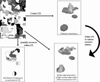
The study of resource use has developed quickly from simple reporting on resources at used points, to describing a vector of average use (Mahalanobus distance; Clark et al. Reference Clark, Dunn and Smith1993), to interpolating the probability of use throughout an animal's travelled area. A utilization distribution (UD; Van Winkle Reference Van Winkle1975) is produced when the amount of time (Samuel & Garton Reference Samuel and Garton1987) or the likelihood of occurrence (Worton Reference Worton1989) are incorporated into home range estimators. This UD is a probability density function (PDF) derived from use point locations that assign a probability of occurrence to each place within the range. It is assumed that the range contains all used places, or 100% of the animal's use (that is, the PDF sums to 1.0). The height of the UD (imagined as the z-axis) can be related to properties of the physical location within an animal's range (the x and y coordinates) underlying the UD (Fig. 1; Marzluff et al. Reference Marzluff, Millspaugh, Hurvitz and Handcock2004). The UD also is the area considered available to an organism and, to the extent that many areas within the UD are used very little or not at all, then analysis of the relative amount of use within the UD approaches an analysis of use to availability.
Calculation of a resource utilization function for a single Steller's jay. First, the jay's location estimates (upper left) are converted into a three-dimensional utilization distribution (UD; upper right) using a fixed-kernel home range estimator. The height of the UD indicates the relative probability of use within the home range. Greater heights indicate areas of greater use as inferred from regions of concentrated location estimates. Second, resource attributes are derived from resource maps within the area covered by the UD. For example, we calculated a continuous resource measure (contrast-weighted edge density; lower right; highest at interfaces between late seral forest and clearcuts or urban areas) and a categorical resource measure (vegetative land cover; lower left) at each grid cell centre within the area of the UD. The height of the UD (relative use × 100) is then related to these local (for example vegetation cover; lower left) and landscape (for example contrast-weighted edge density; lower right) attributes on a cell-by-cell basis with multiple regression techniques that adjust the assumed error term for spatial autocorrelation. Redrawn from Marzluff et al. (Reference Marzluff, Millspaugh, Hurvitz and Handcock2004).

Resource utilization functions (RUFs) are multiple regression equations that relate the intensity of use to resources at a particular location while accounting for the spatial autocorrelation between resources and use, typically within an animal's travelled range (Marzluff et al. Reference Marzluff, Millspaugh, Hurvitz and Handcock2004; Hepinstall et al. Reference Hepinstall, Marzluff, Handcock, Hurvitz and Huzurbazar2005; Millspaugh et al. Reference Millspaugh, Nielson, McDonald, Marzluff, Gitzen, Rittenhouse, Hubbard and Sheriff2006). To the extent that the analysis contains places beyond the UD, it becomes a measure of use to availability within a specified area. If a resource can be mapped, it can be related to use with a RUF (for example the analysis package Ruf.fit written for R by statistician Mark Handcock is available at URL http://csde.washington.edu/~handcock/ruf/). Generally, a RUF is derived for each individual animal, considering the animal as the experimental unit (Otis & White Reference Otis and White1999), and this is then tested for consistency in the correlation between the occurrence of a resource and the relative intensity of its use among individuals.
In this way, a population of American crows (Corvus brachyrhynchos) consistently used lands containing anthropogenic resources more than lands not providing such resources (Neatherlin & Marzluff Reference Neatherlin and Marzluff2004; Withey & Marzluff Reference Withey and Marzluff2009). Steller's jays (Cyanocitta stelleri) generally used forest edges more than forest interiors, but there was significant variation in this use (Marzluff et al. Reference Marzluff, Millspaugh, Hurvitz and Handcock2004). Individuals whose ranges included forest campground interfaces concentrated use along such edges, but individuals without such edges used patchy landscapes but not strictly the edges between the variously-aged forest patches (Marzluff et al. Reference Marzluff, Millspaugh, Hurvitz and Handcock2004). Variability in resource use, contingent upon resource occurrence or type, is a common finding. Dispersing young American robins (Turdus migratorius) consistently used suburban land cover, but song sparrows (Melospiza melodia), spotted towhees (Pipilo maculates) and Swainsons' thrush (Catharus ustulatus) use of forested versus residential lands varied with amount and degree of urbanization as well as road density (Whittaker & Marzluff Reference Whittaker and Marzluff2009).
RUFs depend on accurate derivation of the UD. As with any interpolation, the estimation of the UD should improve with the number of accurately recorded locations. Global positioning system (GPS) technology has greatly expanded ability to document used places over the full geographic extent of an animal's range, often at a fine temporal resolution. Recent studies suggest that RUFs are especially applicable to animals with small home ranges (Long et al. Reference Long, Muir, Rachlow and Kie2009). Therefore, here we illustrate the RUF approach for wide-ranging animals, drawing on abundant remotely-obtained relocations of cougars (Puma concolor).
The cougar is a solitary, far-ranging carnivore that occupies a broad range of habitats in temperate and tropical environments throughout the western hemisphere. Despite a lack of measurement, the presence of stalking, resting, and security cover for the capture and consumption of prey and rearing of young is consistently cited as a prerequisite for use (Seidensticker et al. Reference Seidensticker, Hornocker, Wiles and Messick1973; Koehler & Hornocker Reference Koehler and Hornocker1991; Williams et al. Reference Williams, McCarthy and Picton1995; Dickson & Beier Reference Dickson and Beier2002; Dickson et al. Reference Dickson, Jenness and Beier2005). Cover is easy to conceptualize, but can be difficult to measure. Cover is a combination of biotic and abiotic features that help to decrease visibility, conceal the predator and increase the vulnerability of prey. Cover includes both the over and understorey vegetation, physical structure of the habitat and topography (Seidensticker et al. Reference Seidensticker, Hornocker, Wiles and Messick1973). Cougars are adaptable predators that consume prey as small as deer mice (Peromyscus spp.) and as large as moose (Alces alces). Accordingly, cover requirements vary dependent upon the prey being hunted and may be more abundant or advantageous within particular habitat types (for example riparian; Dickson & Beier Reference Dickson and Beier2002) or landscape configurations (such as edges; Altendorf et al. Reference Altendorf, Laundre, Lopez and Brown2001). As a top-tier carnivore, the availability of high-quality forage and browse for ungulate prey may be important landscape features for cougars (Goh Reference Goh2000).
We illustrate the issues, challenges and benefits of resource use studies, especially considering large samples from wide-ranging animals. We (1) address the computational challenges inherent in deriving UDs from thousands of use points and RUFs from hundreds of thousands of use and resource estimates; (2) investigate how selection of the kernel smoothing parameter, critical to the derivation of the UD (Gitzen et al. Reference Gitzen, Millspaugh and Kernohan2006), affects results; and (3) compare insights into resource selection derived by relative use versus use:availability studies.
METHODS
We examined cougar resource use in a 3500 km2 study area in the suburban, exurban and wildland portions of King and Snohomish Counties (Washington, USA; 590 000 E, 5260 000 N or 49°29′14″ E, 121°48′19″ N). Elevations extend from 10 to 2005 m and mean annual precipitation ranges from 142 cm in the west to 257 cm in the east occurring primarily between 1 October and 1 July (Western Region Climate Center 2009). Douglas-fir (Pseudotsuga menziesii), western hemlock (Tsuga heterophylla) and Pacific silver fir (Abies amabilis) forest associations are the dominant habitats on the landscape with trees ranging in age from 1–300 years with a majority found in seral stages less than 50 years old (Koehler & Pierce Reference Koehler and Pierce2003). Land ownership is a composite of state, federal, municipal and private holdings managed for timber production, water resources, multiple-use, wilderness and private residential. The western portion of the study area (c.1000 km2) is heavily urbanized with human densities as high as 850 people per km2 and small highly-fragmented forest patches that are used less frequently by cougars (Kertson Reference Kertson2010). Cougars within the study area prey primarily on black-tailed deer (Odocoileus heminous columbianus), beaver (Castor canadensis), elk (Cervus elaphus), raccoon (Procyon lotor) and mountain beaver (Aplodontia rufa; Kertson Reference Kertson2010).
We captured 32 adult and subadult cougars during November 2003–December 2008 using trained dogs and large steel-cage traps baited with cougar-killed or road-killed deer and elk (Spencer et al. Reference Spencer, Pierce, Schirato, Dixon and Richards2001). Captured individuals were immobilized with a 10:1 mixture of ketamine hydrochloride and xylazine hydrochloride (Plum Creek Pharmaceuticals, Amarillo, TX, USA) administered intramuscularly at a dosage of 8.8 mg kg−1 ketamine and 0.88 mg kg−1 xylazine via a 3.0 ml plastic dart fired from a CO2-powered dart gun (Dan Inject North America, Fort Collins, CO, USA; Spencer et al. Reference Spencer, Pierce, Schirato, Dixon and Richards2001). Immobilized cougars were given a physical examination, ear tagged and outfitted with a 600 g GPS radiocollar (Model GPS Plus-2, Vectronics Aerospace, Berlin, Germany; Model GPS-Telus and GPS-Simplex, Televilt, Lindesberg, Sweden). GPS radiocollars were programmed to attempt a satellite fix for 180 s, six times per day (every 4 h) in an attempt to maximize collar performance and data acquisition (Cain et al. Reference Cain, Krausman, Jansen, Morgart and Krausman2005; DeCesare et al. Reference DeCesare, Squires and Kolbe2005; D'Eon & Delparte Reference D'Eon and Delparte2005; Lewis et al. Reference Lewis, Rachlow, Garton and Vierling2007). Cougars were located 1–2 days per week using ground-based radiotelemetry techniques (Mech Reference Mech1983) and we remotely downloaded GPS data sets every 14–21 days using Uhf bi-directional communication technology.
We focused our analysis on 17 cougars with >200 GPS relocations per year (1 Jan–31 Dec) and 20 cougar-years of data. For three cougars with multiple years of data, we considered each year independent because annual space use patterns shifted likely because of high mortality in the population, changes in the social status of individual cougars and landscape alteration from residential development and commercial logging (Kertson Reference Kertson2010). Cougars had an average of 896 GPS relocations (SD = 524) and collars had an average fix rate of 65% (SE = 5) yielding one successful fix every 6.2 h with an average positional dilution of precision (PDOP; a measure of error) = 5.1 (SE = 0.2). Cougars moved an average of 1214 m (SE = 176, n = 17) between fixes.
Selection of the kernel smoothing parameter (h) is critical to estimation of the UD and analysis with the RUF (Kernohan et al. Reference Kernohan, Gitzen, Millspaugh, Millspaugh and Marzluff2001; Millspaugh et al. Reference Millspaugh, Nielson, McDonald, Marzluff, Gitzen, Rittenhouse, Hubbard and Sheriff2006). This parameter, also termed the bandwidth, is a measure of the range of spatial dependence within the UD. We compared h values and resulting UDs using three bandwidth selection techniques: plug-in (hPI), least squares cross-validation (hLSCV) and reference (hREF). The reference bandwidth often is used for objectivity and computational simplicity (Worton Reference Worton1989). Least squares cross-validation methods are objective (Kernohan et al. Reference Kernohan, Gitzen, Millspaugh, Millspaugh and Marzluff2001; Gitzen et al. Reference Gitzen, Millspaugh and Kernohan2006), but can be problematic for GPS data sets because they require significant processing time, or may not be estimated for distinctly bimodal ranges, given the computational procedure of the hLSCV calculation (Silverman Reference Silverman1986). Our processing for individuals with greater than 1000 relocations required >24 hrs per individual with 512 megabytes of random access memory (RAM). The plug-in method is considered superior to hLSCV techniques for most distributions (Wand & Jones Reference Wand and Jones1995; Gitzen et al. Reference Gitzen, Millspaugh and Kernohan2006), but the method is not readily available in kernel software and is used infrequently. We calculated bivariate hPI values using the hpi function of the KernSmooth package available in R (Wand Reference Wand2006). We used the ANIMAL MOVEMENTS extension available in ArcView 3.3 (Hooge & Eichenlaub Reference Hooge and Eichenlaub1997) to estimate univariate hLSCV values and the Home Range Tools extension (HRT; Rogers et al. Reference Rodgers, Carr, Beyer, Smith and Kie2007) available for ArcMap 9.2 to derive hREF.
We estimated fixed-kernel home ranges (UDs) using Fixed-Kernel Density Estimator in the Hawth's Tools extension (Beyer Reference Beyer2004) for ArcMap 9.2. We output grids for each UD with a 30 × 30 m cell size to match the spatial resolution of our landscape data. We created a 99% volume polygon using Percent Volume Contour (Beyer Reference Beyer2004) and excluded all cells outside of this boundary. Thus, we are analysing variation in use within the home range and assume that all points within the home range received some actual use. The entire home range is considered available. We converted kernels from density to volume using Percent Volume Contour (Beyer Reference Beyer2004) and Feature to Raster in ArcTool Box to rescale use values between 1 (lowest use) and 99 (highest use) based on the volume (height) of the UD at each cell (Marzluff et al. Reference Marzluff, Millspaugh, Hurvitz and Handcock2004). We compared UD surfaces and use values from different bandwidths by calculating the volume of intersection (Kernohan et al. Reference Kernohan, Gitzen, Millspaugh, Millspaugh and Marzluff2001) and the linear correlation in use among 50 000 randomly selected points from the hPI, hLSCV and hREF UDs.
Research identifying landscape characteristics used by cougars in lowland Douglas fir/western hemlock forests of the Pacific Northwest has not been conducted, so we selected metrics we hypothesized might be good predictors of use based on our observations of cougar ecology and behaviour. Cougars in western Washington routinely preyed upon beavers and black-tailed deer in close proximity to water (streams, rivers, wetlands and lakes) and deer in early successional forests. Using these observations, we selected three variables for inclusion in our model: distance to water (m), per cent clearcut and regenerating forest (%2) and slope (degrees). These landscape characteristics are the covariates of use that we consider to be indicative of ‘resources’ for this paper (Manly et al. Reference Manly, McDonald, Thomas, McDonald and Erickson2002). Distance to water was derived using high resolution imagery from the National Hydrography Database (URL http://www.nhd.usgs.gov) and Spatial Analyst Euclidean Distance in ArcMap 9.2. Slope was derived using Spatial Analyst Slope Surface and the United States Geological Survey's 10 m digital elevation model for UTM Zone 10 (Kertson Reference Kertson2010). We derived per cent clearcut and regenerating forest using the methods outlined in Hepinstall et al. (Reference Hepinstall, Alberti and Marzluff2008a, Reference Hepinstall, Marzluff, Alberti, Millspaugh and Thompson IIIb). We predicted that use would increase with increases in per cent clear cut and regenerating forest and would be inversely related to distance to water (use increases with decreasing distance) and slope (decreases with increasing slope).
We built the spatially explicit data file required by Ruf.fit using Hawth's Tools. The FOCAL PATCH extension used in Marzluff et al. (Reference Marzluff, Millspaugh, Hurvitz and Handcock2004) for this purpose is unavailable for ArcMap 9.2, but Hawth's Tools offers a suite of tools that perform the same functions as FOCAL PATCH, with the added advantage of fixed-kernel home range estimation using a bivariate h. We used Generate Regular Points (Beyer Reference Beyer2004) to create a grid of x- and y- coordinates centred on each pixel within the 99% UD. We used the Sample tool in ArcTool Box to simultaneously extract relative use and covariates associated with resource units. Although there are benefits of increased resolution of the UD, these are offset by the challenges of organizing and analysing the resultant large data sets. Male cougars in western Washington routinely traverse home ranges larger than 400 km2 (Kertson Reference Kertson2010) resulting in a 99% UD containing > 600 000 30 × 30-m cells. Geographic information systems software is capable of completing many necessary functions for the RUF, but processing time for many tasks can be large. Exported tables create additional challenges because files are not easily managed in many database software packages (for example the maximum number of 65 536 table rows is exceeded in Excel 1997–2003; Microsoft Corporation, Redmond, WA, USA). Software upgrades (such as Excel 2007) eliminate this problem for most datasets, but not all. There are no size limitations for importing and analysing files in R, but use of Ruf.fit may be hampered by computer processing and memory capabilities.
Subsampling of the UD for RUF analysis might be useful if computing power is limited, but we have found subsampling to be unnecessary with the increased processing speed and RAM available with most newer computers. For example, we were able to estimate a RUF with 11 coefficients from 2.2 million lines of data in approximately 3 h using a desktop computer with 6 gigabytes of RAM. We used the Ruf.fit package in R to output unstandardized and standardized resource coefficients and associated standard errors for each bandwidth method. We used standardized coefficients to construct 95% confidence intervals for each individual to determine the number of cougars with use significantly associated with each covariate (Marzluff et al. Reference Marzluff, Millspaugh, Hurvitz and Handcock2004). We mapped predicted cougar selection throughout the study area from the averaged unstandardized coefficients of our sample and three individuals to illustrate the utility of RUFs to capture variation in resource use among individuals (Marzluff et al. Reference Marzluff, Millspaugh, Hurvitz and Handcock2004). We tested for statistical differences (α = 0.05) between RUF standardized coefficients derived from each bandwidth method using multiple comparison techniques controlling for Type I error with Tukey's honestly significant difference method (Zar Reference Zar1999).
RESULTS
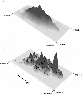
The UDs from VHF and GPS relocations were strikingly different (Fig. 2). UDs from small samples of relocations had few peak high-use areas because the few relocations were well spaced. Interpolation during the kernelling process defined the UD for such minimally sampled individuals. For example, a female cougar UD estimated from 55 Vhf radiotelemetry relocations was more reliant on interpolation between points than nuanced fitting among points of actual use than was her UD estimated from 2358 GPS relocations (Fig. 2).
Utilization distributions of an adult female cougar derived from (a) 55 ground-based Vhf relocations (black dots) recorded from 23 January 2006 to 29 April 2008 and (b) 2358 GPS relocations (black dots) obtained from 13 February 2007 to 29 April 2008. Utilization distributions were estimated using the bivariate plug-in h value provided by the KS package in R statistical software and the fixed kernel density estimator in the Hawth's Tools extension for ArcMap 9.2 (Beyer Reference Beyer2004).

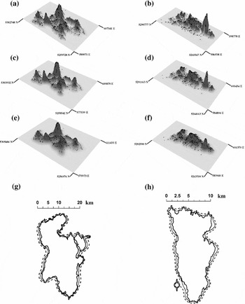
Bandwidth selection methods produced h values that varied up to three-fold for individual animals. The estimated range of spatial dependence was smallest, meaning resulting UDs were most jagged, using the plug-in method and greatest using the reference bandwidths (Table 1). Plug-in UDs were less similar to other methods with lower coefficients of determination and volumes of intersection (Table 1, Fig. 3). Visual examination confirmed that plug-in UDs were more jagged with many pronounced peaks and valleys compared to the other methods (Fig. 3). UDs from reference bandwidth were least defined, but relative use of a given point was essentially unchanged. The average number of cells in 99% UDs ranged from 588 615 (hPI) to 826,508 (hREF; Table 1).
Comparison of the utilization distributions (UDs) for 17 cougars derived from bivariate plug-in (PI), least squares cross-validation (LSCV), and reference (HREF) bandwidth selection methods. Mean smoothing parameter values (h), and sizes (number of 30 × 30 m cells) define the extent and rugosity of the UD, respectively. Slopes and coefficients of determination (r2) quantify the similarity in the heights of the UDs derived by each method for individual cats at 50 000 random points within each animal's actual home range. Volume of intersection (VI) measures the total congruence in UD volumes despite using different bandwidth selection techniques for each individual cat in a spatially-explicit fashion. aPI: LSCV, bPI: HREF, cLSCV: HREF.

Utilization distributions for an adult male and female cougar estimated using GPS relocations (black dots), the fixed kernel density estimator tool in the Hawth's Tools extension (Beyer Reference Beyer2004) of ArcMap 9.2, and plug-in: (a) male, (b) female; least squares cross-validation: (c) male, (d) female; and reference: (e) male, (f) female bandwidth selection methods. Two-dimensional overlap of utilization distributions for the (g) male and (h) female cougar provides an alternative perspective to view differences between the shape and spatial extent of utilization distributions derived from different bandwidth selection methods (plug-in: solid line; least squares cross-validation: small dashes; reference: larger dashes).

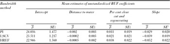
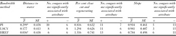
The method of estimating the UD influenced the RUF coefficients only slightly. Unstandardized RUF coefficients were similar between bandwidth methods and subsequent predictive maps of cougar use were similar (Table 2). Unstandardized coefficients were supportive of our predictions based on known ecology and behaviour because cougars increased use in areas close to water, areas with a higher percentage of clear-cut and regenerating forest, and those with lower slopes (Table 2). Each bandwidth selection method captured similar levels of variation in resource use by cougars (Table 3) and there were no statistically significant differences between average standardized resource coefficients derived from each bandwidth method (distance to water: F(2,57) = 0.30, p = 0.75; per cent clear cut and regenerating forest: F(2,57) = 0.29, p = 0.75; and slope: F(2,57) = 0.05, p = 0.95). The relative importance of covariates differed slightly between the bandwidth selection techniques. In each case distance to water was least important (smallest average coefficients of use) and least consistent across animals (nearly equal numbers of cats had significant negative coefficients of use as did those having significant positive coefficients of use; Table 3). Slope, and percentage of clear-cut and regenerating forest were more strongly and consistently associated with cougar use than was distance to water regardless of bandwidth selection method. However, clear-cut and regenerating forest was identified as the most important variable affecting use for least squares cross validation and reference bandwidth methods, whereas slope was most important for the plug-in method (Table 3).
Resource utilization functions (RUFs) for cougars in western Washington derived from plug-in (PI), least squares cross-validation (LSCV) and reference (HREF) bandwidth selection methods. †Conservative standard errors were estimated with measures of inter-animal variation derived using methods in Marzluff et al. (Reference Marzluff, Millspaugh, Hurvitz and Handcock2004).

Standardized RUF coefficients (β), standard errors and inter-animal consistency of resource use for 17 cougars (n = 20 cat-years of data) in western Washington, derived from plug-in (PI), least squares cross-validation (LSCV) and reference (HREF) bandwidth selection methods. *Differences in sign between standardized and unstandardized coefficients may occur for non-significant predictors as each is estimated during separate independent runs using an iterative process in Ruf.fit.

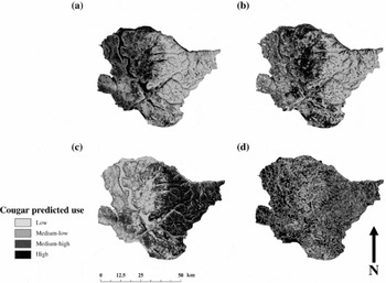
The majority of cougars used each resource significantly regardless of bandwidth selection method, but individual space use patterns were highly variable (Table 3). Inter-animal variation accounted for an average of 99.91% of the total variation for each estimated coefficient (SD = 0.09, n = 9) and use by the population was only significant for slope with plug-in and least squares cross-validation and per cent clear-cut and regenerating forest using least-squares cross-validation and reference bandwidths (namely other 95% confidence intervals for averaged coefficients included 0; Table 3). Maps from the averaged unstandardized coefficients illustrate how this individuality is largely lost when predicting use for the population (Fig. 4). The average RUF coefficients were influenced primarily by males (65.00% of sample) that used early successional forests (61.15 ± 0.00%), areas close to water (61.15 ± 0.00%), and those with lower slopes (71.66 ± 11.92%; Fig. 4b). Females (35.00% of the sample) and individuals that used steep, high-elevation areas with limited amounts of early successional forest (Fig. 4c) or those with a territory in a portion of the study area where cougar capture efforts were limited (Fig. 4d).
Maps of predicted cougar use for our 3500 km2 study area in western Washington based on resource utilization functions derived from (a) our sample of 17 cougars, (b) an adult male representative of the majority of individuals in our sample, (c) a relatively unique adult female that used steep high elevation areas with limited amounts of early successional forest, and (d) an adult female that used a portion of the study area where few cougars were captured.

DISCUSSION
The study of resource selection by wild free-ranging animals has proceeded by measuring resource use and interpreting use from the perspective of what researchers determine is available to the animal. While the concept of availability is inherently important and interesting, we suggest ability to infer resource importance is better served by more careful study of resource use. Characterizing covariates among resource units that are frequently used and contrasting them with resource units that are used less frequently enables the results of resource selection in the wild to be viewed and provides managers with empirically rooted underpinnings for their actions.
In our study, we were able to quantify the highly individualistic resource use by a generalist wide-ranging predator. Despite this individuality there was a tendency for cougars to concentrate their activity near vegetation likely to hold prey (clearcuts and regenerating forests) and rarely to use steep mountain slopes. For our cougars, most differences in resource use could be explained by differences between sexes or age classes. We suggest that the next approach to meet management needs would be to map predicted use from RUFs estimated for these specific demographic classes.
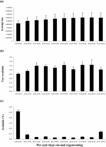
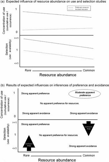
Average use of resources provided a simple description of animal activity relative to resource availability. Average use equals the expected use per resource unit for a given resource covariate. In essence this is a refined selectivity index that accounts for variation in the intensity of observed resource use. Elsewhere we termed this the ‘concentration of use’ (Neatherlin & Marzluff Reference Neatherlin and Marzluff2004) because it indicates how use varies among resources. As predicted, a majority of cougars concentrated their use in resource units with abundant regenerating forest (Fig. 5a). But typical selection indices (use:availability) suggested counter-intuitive selection for moderately-used rare resources (Fig. 5b, c). We expect such results to be common. If animals strongly select the resource of interest, measuring use relative to availability will likely overestimate the importance of rare resources and underestimate the importance of common resources (Fig. 6a). This is simply inevitable, despite correct identification of frequent use, because rare resources have low availability while common ones have high availability. Scaling frequent use by low availability provides ‘evidence’ of strong selection, while scaling frequent use by high availability reduces the ‘evidence’ for selection. Neither answer is correct. Likewise if animals strongly avoid rare or common resources, this avoidance is over- or under-estimated, respectively in use:availability studies. Detecting avoidance of rare resources and selection of common resources are both difficult given the mathematics of scaling use to availability (Fig. 6b).
Comparison of (a) average use per cell, (b) selection and (c) availabilityof clear cut and regenerating forest (%) for 17 cougars (n = 20 cat-years of data) in western Washington. Average use per cell was calculated as the total proportion of each individual's utilization distribution in the resource class divided by the total number of cells in that class within the home range. Average selection was calculated as the mean of each individual's use (proportion of each individual's GPS relocations) divided by available (proportion of cells in the landscape metric class within each cougar's home range). Average availability was estimated by dividing the number of cells in each class by the total number of cells for each cougar's home range. Bars are the standard error associated with each class for the 20 samples.

Likely insights into animal resource selection derived from studies of variation in resource use (refined ‘selection’ index accounting for relative use) and resource use relative to resource availability (typical ‘selection’ indices). (a) Expected influence of resource abundance on use and selection studies. (b) Results of expected influences in inferences of preference and avoidance. We expect resource occurrence (or naïve availability) to influence typical selection metrics more than use metrics because division by rare resource availability negates avoidance (low use) and division by common resource availability negates selection (high use). We show these effects in the lower panel of (b) as linear functions of resource availability, but they may be nonlinear. Average use of rare and common resources should reflect selection or avoidance because use is averaged per unit of resource. The potential influence of resource abundance leads to three areas of possible confusion (b). The first, in studies of resource use, is the ability to detect actual resource selection from frequent use of common resources. We expect some devaluation of cumulative use because some areas of common resources may not be used; note also slight decline in selection line in (a). The second and third, in studies of resource use:availability, reflect the devaluation of avoidance of rare and selection of common resources noted in (a).

Studies of relative resource use are affected by resource abundance to a lesser degree. Inferring selection of a resource by its average frequency of use correctly provides evidence of avoidance (infrequent use) regardless of resource abundance (for example Fig. 6a). Inferring selection from actual average use should be accurate when resources are rare and frequent use is divided by a small area of resource occurrence (Fig. 6a). As in use:availability studies, selection for widely distributed resources is difficult to correctly identify and avoidance of abundant resources should be obvious (Fig. 6b).
This likely matters little for the manager because resources that may or may not be selected, but are used, are also abundant. For managers moderately common to rare resources may need the most attention. Here the study of relative use likely outperforms the study of use:availability (for example Fig. 5). Rare resources that are frequently used will be recognized as important in both types of studies (Fig. 6a). Rare resources that are actually avoided, however, should be easier to identify with use than with use:availability studies because low probability of use is averaged over a small area rather than discounted by an equally low availability (leading selection to suggest use is proportional to availability; Fig. 6b). The assumptions of use:availability studies and relative use studies clearly influence conclusions, and inductive reasoning of these effects should be subjected to rigorous study.
The possibility of resource selection studies to under- or overestimate actual animal resource preference, especially because of the underlying abundance and distribution of resources in nature, suggests the need to more fully understand patterns of resource use by animals. Technology is increasing our ability to define use patterns and derive UDs with less interpolation, but even a true UD, derived from perfect knowledge of animal travels, will not tell a manager if a common resource is really preferred or simply often used. Quantifying and managing for frequently used resources may be sufficient for conservation and regulated harvest, but a greater understanding of the behaviours underlying resource use help reveal actual preference in field settings (Marzluff et al. Reference Marzluff, Knick, Millspaugh, Millspaugh and Marzluff2001). Knowing how resources are used would establish whether rare resources are truly avoided or simply used for rare, but critical behaviours (like obtaining trace minerals or encountering mates), and if common resources provide for a diversity of uses summing to extreme importance, or simple redundancy. Remotely-sensed relocations rarely provide information as to what the animal was doing. Therefore, to fully benefit from the increased resolution of remotely monitoring where animals travel, remote monitoring of behaviour along the route needs to be improved.
Considering variation in the amount of resource use to gauge resource preference, rather than considering resources as simply used or not and then inferring resource preference from this use relative to availability, is a conceptual advancement (Long et al. Reference Long, Muir, Rachlow and Kie2009). As ability to resolve the pattern of variation in use (the true UD) improves, this conceptual advancement may yield practical benefits. Cougar UDs are highly resolved, affected little by choice of smoothing parameter, and reliable at confirming and mapping resource use expected based on detailed on-the-ground tracking and investigation of foraging behaviour. Investigations of resource use by jays informed managers concerned about the impact of jays on rare species (Raphael et al. Reference Raphael, Evans, Marzluff and Luginbuhl2002), and our cougar analyses may inform state managers concerned with sustainable harvests and conservation of predators in urbanizing areas.
Selecting the proper smoothing factor to reveal a defensible biologically-relevant UD is a combination of science and art. Objective methods to select h may not faithfully reveal the pattern of use apparent in the actual point locations, so subjective methods may be needed. In our examples this was not necessary. The objective plug-in method, while less commonly used by researchers than easy to calculate reference or least-squares methods, is analytically strong (Gitzen et al. Reference Gitzen, Millspaugh and Kernohan2006), now available to users of R and produced UDs that best represented the variation in use evident within our wide-ranging remotely-sensed cougar home ranges. Our examples suggest, that while the smoothing factor certainly influences the extent and ruggedness of the UD, it does not grossly affect the determination of relative use or the relationship between relative use and resource occurrence. UDs created using smoothing factors that varied by a factor of three were spatially concordant and produced similar RUFs. The importance of frequently or rarely used resources was especially resilient to variation in the smoothing factor. A larger smoothing factor might better represent the coarse scale of locations typical of early studies reliant on VHF transmitters.
The influence of smoothing on the derivation of resource use functions should be studied in other situations. In this study, we were less concerned with resolving the UD, especially when large samples of points may be smoothed with rigorous methods like the plug-in, than we were with understanding if and how our observation points were biased. GPS error is predictable and its bias can be removed (Frair et al. Reference Frair, Nielsen, Merrill, Lele, Boyce, Munro, Stenhouse and Beyer2004; Lewis et al. Reference Lewis, Rachlow, Garton and Vierling2007), but we have not investigated this in our system.
The understanding of resource preference is elusive. It may never be possible to demonstrate preference in the field because resources are rarely equally available and animals' decisions are difficult for humans to perceive. But resource importance can be measured with greater resolution by clear documentation of resource-use patterns and thorough understanding of how resource availability and occurrence influence perceptions of resource choice. As empiricists, we hold firmly to the importance of understanding variation in resource use. We here demonstrated some of the challenges and opportunities in the study of resource use by wide-ranging animals tracked with remote GPS transmitters. To manage the resources desired by humankind and needed by so many other species will require lasting collaborations between biometricians and field ecologists.