INTRODUCTION
Individual crop and whole farm modelling has become an important tool for exploring how the environment and human behaviour affect agricultural systems. This simulation of on-farm circumstances makes it possible to incorporate hypothetical scenarios including plant genetics, climate and farm management profiles. Simulation is a worthwhile alternative to creating the intended conditions in controlled environments, e.g. experiments in climate chambers and under real conditions. Hypothetical plant genetics, for one, are impossible to demonstrate in this regard.
With the global population reaching 7 billion and a global atmospheric carbon dioxide (CO2) concentration of 400 ppm (Ewald Reference Ewald2013), concerns about world food security being threatened by anthropogenic climate change have not waned (Högy & Fangmeier Reference Högy, Fangmeier and Hoffman2013). On the contrary, as stated by van Ittersum et al. (Reference Van Ittersum, Cassman, Grassini, Wolf, Tittonell and Hochman2013), the prognosis has deteriorated, putting more pressure on the scientific community to provide sound projections of agricultural production in the coming decades. To this end van Ittersum et al. (Reference Van Ittersum, Cassman, Grassini, Wolf, Tittonell and Hochman2013) have also emphasized the importance of crop simulation models at daily resolution with flexible simulation of management actions. The adaption of agriculture to global change is of interest to a range of stakeholders including researchers, policy makers and farmers (Bizikova et al. Reference Bizikova, Crawford, Nijnik and Swart2014), and crop modelling is an effective means of evaluating possibilities (Matthews et al. Reference Matthews, Rivington, Muhammed, Newton and Hallett2013). The goal is to elucidate some of the mechanisms by which agricultural production will be adjusted to future environmental conditions.
Calibration of crop models benefits from as much detail as can be provided by experiments and observations containing the information that goes into simulation. The current study demonstrates some of the advantages of precise, relevant data collection by using it to generate an outlook on crop performance, including plant development and potential yield. The premise is that the better past observations are replicated, the more reliable are projections into the future. The current study builds upon decades of work modelling winter wheat, summer and winter barley and maize with CERES (Jones & Kiniry Reference Jones and Kiniry1986) and all four plus winter rapeseed with GECROS (Yin & Van Laar Reference Yin and Van Laar2005). These crops cover almost half of Europe's arable land, three-quarters of Germany's and four-fifths of that in Baden-Württemberg (Eurostat 2013) making their economic and nutritional importance extreme. By calibrating and validating simulations of these crops with data from various sources, subsequent simulations of their cultivation 30 years into the future can be viewed with confidence.
The current study includes projected future farmer behaviour, which, as with crop modelling, is valuable for scenario analysis and bound to realistic simulations of reality. Performance of cropping actions, especially planting, has a noticeable impact on crop performance and hence is crucial to reliable simulation (Leenhardt & Lemaire Reference Leenhardt and Lemaire2002; Sacks & Kucharik Reference Sacks and Kucharik2011; Waha et al. Reference Waha, van Bussel, Müller and Bondeau2012). The current study mimics the decision-making process that drives the timing of field-level actions including planting and harvesting, based on farmer reactions to environmental conditions. This includes farmers responding to current weather and soil conditions on a daily basis, as well as learning from historic patterns to generate expectations and steer behaviour. Again, accurate replication of historic, site-specific observations instils confidence in hypothetical scenarios. The current study presents the latest improvements to FarmActor as integrated with the agro-ecosystem model Expert-N (Priesack Reference Priesack2006). The improved model is applied to an arable region of south-west Germany (Kraichgau), contrasting sharply to the Swabian Alb of the previous application (Aurbacher et al. Reference Aurbacher, Parker, Calberto Sánchez, Steinbach, Reinmuth, Ingwersen and Dabbert2013). Projections of adaptive management and consequent crop phenology and likely yields are made using simulated future weather scenarios.
MATERIALS AND METHODS
Study area
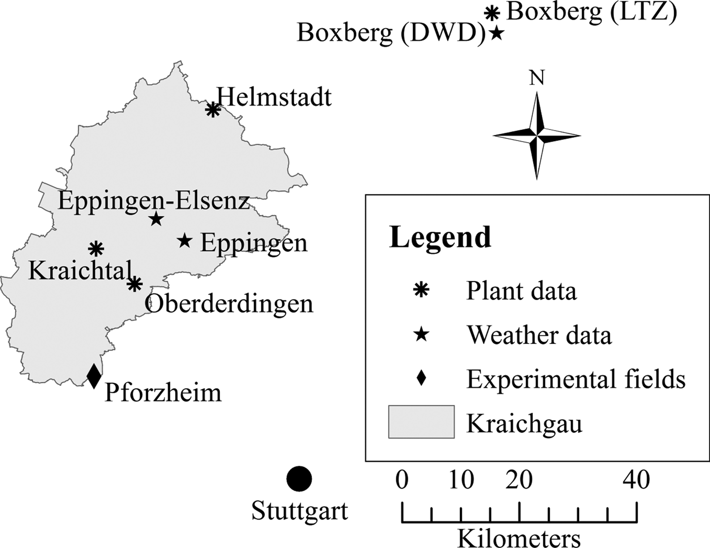
The Kraichgau (c. 1400 km2) is a region of rolling hills with thick loess soils located between the Rhine and Neckar Rivers. The region is characterized by a mild climate with an annual mean temperature of 9·1 °C, making it one of the warmest regions in Germany. Mean annual precipitation ranges from 720 mm (in the west) to 830 mm (east and south). The Kraichgau is in Karlsruhe County (Regierungsbezirk) and composed of Karlsruhe Rural (0·38), Heilbronn (0·23), Rhein-Neckar (0·10) and Enzkreis (0·10) districts (Kreise). It represents prime Central European cropland. Figure 1 shows the study area and key locations within the state of Baden-Württemberg.
Map of study area with key locations.

Experimental fields
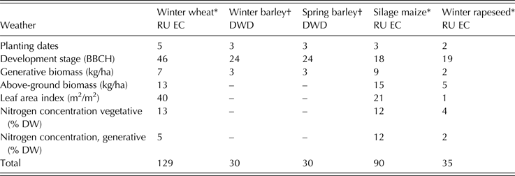
The farm ‘Katharinentaler Hof’ (48°55′N, 8°42′E, 319 m a.s.l.) is located north of Pforzheim at the southern edge of the Kraichgau. Three research units or ‘eddy-covariance stations’ (RU EC1-3) were outfitted on separate fields (16–24 ha) to record weather and soil conditions at half-hourly resolution, subsequently aggregated to daily values; a detailed description is given in Ingwersen et al. (Reference Ingwersen, Steffens, Högy, Warrach-Sagi, Zhunusbayeva, Poltoradnev, Gäbler, Wizemann, Fangmeier, Wulfmeyer and Streck2011) and Gayler et al. (Reference Gayler, Ingwersen, Priesack, Wöhling, Wulfmeyer and Streck2013). The weather data recorded at experimental fields was used for calibration of the crops grown on them. Winter wheat, silage maize and winter rapeseed were grown on four fields in 2009 and three fields in 2010/2011 as part of normal crop rotations, grown over five, three and two seasons, respectively, to provide bi-weekly or monthly plant development (BBCH 1997) and leaf area index (LAI, 0+) measurements plus intermittent measurements on whole plant and generative biomass partitioned dry weight (DW, kg/ha) and nitrogen (N) concentration (% DW) (Högy et al. Reference Högy, Zörb, Langenkämper, Betsche and Fangmeier2009; Ingwersen et al. Reference Ingwersen, Steffens, Högy, Warrach-Sagi, Zhunusbayeva, Poltoradnev, Gäbler, Wizemann, Fangmeier, Wulfmeyer and Streck2011). Table 1 shows the number of plant measurements provided by field surveys for crop model calibration.
Weather source and number of data sets per observation and crop used for crop model calibration
DW, dry weight.
* Own field observations at research unit (RU) eddy covariance (EC) stations.
† Source: LTZ (2013).
The differences between plot-measured and farmer-reported yields were averaged by crop and taken as a measurement bias to be applied to crop model results. Modelled yields were thus corrected by −19% for wheat, −18% for rapeseed and +4% for maize.
Supplemental data
The German Weather Service maintains a network of both weather (DWD 2012a) and phenological (DWD 2012b) observatories, often in close enough proximity to allow derivation of causal relationships between them (Menzel Reference Menzel and Schwartz2013). The DWD weather station at Eppingen was moved to a nearby location in 2002 and renamed Eppingen-Elsenz. Records from the two stations were merged and deemed to be from one location. Phenological observations indicate the local onset of crop phases, including the artificial ones used below, planting and harvest. The DWD Phenology station at Oberderdingen was chosen because of its location between the experimental fields and Eppingen.
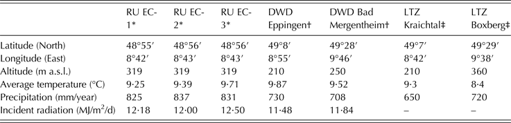
Experimental fields were not sown with summer or winter barley during the period used for calibration so less detailed data, limited to development stage and final crop yield, were taken from Baden-Württemberg state field trial stations as close as possible to the experimental fields (LTZ Augustenberg 2013). One advantage provided by the LTZ data is multiple years of trials using specific cultivars, so that barley cvar Braemar and cvar Lomerit were chosen as representative of spring and winter cultivars, respectively, in the region. Experimental data covering several years were available for spring barley at the Kraichtal site, close enough that soil parameters from a Katharinentaler Hof field and DWD weather from Eppingen were used for calibration. For winter barley, the nearest source of LTZ experimental data was in Boxberg (Fig. 1). For this site, soil data were derived from the Soil Map of the Federal State of Baden-Württemberg (LGRB 1997) and weather data were taken from the nearest station (Bad Mergentheim) with records of each weather variable needed for simulation. The DWD phenological records for spring barley end in 1990, so they were amalgamated with planting and harvest data from various LTZ trials sites for validation 1991–2010. Table 2 gives a statistical summary of locations with sources of data.
Summary statistics (2010/2011) on data source locations
* Sources: own field observations from research unit (RU) eddy covariance (EC) stations.
† DWD (2012a).
‡ LTZ Augustenberg (2013).
Simulated field management and behavioural paradigms
Learning from several years of weather designates the onset of planting periods each year, during which daily soil moisture, air temperature and precipitation, plus temperatures over the last 3 days, serve as action triggers (Aurbacher et al. Reference Aurbacher, Parker, Calberto Sánchez, Steinbach, Reinmuth, Ingwersen and Dabbert2013). Following Olesen et al. (Reference Olesen, Børgesen, Elsgaard, Palosuo, Rötter, Skjelvåg, Peltonen-Sainio, Börjesson, Trnka, Ewert, Siebert, Brisson, Eitzinger, van der Fels-Klerx and van Asselt2012) maximum temperature values, daily and over 3 days prior were added as criteria for autumn sowing. The justification for this mechanism is the perceived risk on the part of a farmer that excessive temperatures are likely to result in over-development before winter dormancy, while also being conducive to insect, pathogen and weed growth.
Harvest is subject to a set of simultaneously evaluated feasibility criteria including crop growth stage (GS 92 for seed crops and GS 88·8 for silage maize; BBCH 1997), soil trafficability (water content below field capacity) and daily precipitation (0 mm on the day of harvest). In seed crops a proxy for grain moisture content is a combination of minimum pre-period temperature and maximum precipitation (8 °C and 10 mm over 3 days), to capture the importance of drying costs.
Reproducing farmer behaviour previously relied on fixed trigger values throughout allotted time windows with derestriction occurring at the end of these periods in order to prevent failed actions (Aurbacher et al. Reference Aurbacher, Parker, Calberto Sánchez, Steinbach, Reinmuth, Ingwersen and Dabbert2013). Two alternative decision-making paradigms were created to improve the accuracy of simulated management.
‘Shifting’ triggers
A mechanism for shifting triggers was developed so that each day after the start of the planting period, triggers were constantly relaxed to a calibrated degree. It was a daily check whether t: t ≥ base − shift × day for a minimum trigger, or: t ≤ base + shift × day for a maximum trigger, each day during the time window. This can be very restrictive early in the period when only exceptionally favourable combinations of environmental conditions will permit action, and also allow progressively sub-optimal combinations late in the period, facing the risk of late or failed action.
‘Fuzzy’ triggers
Fuzzy logic has already been applied to crop modelling (Wieland et al. Reference Wieland, Mirschel, Nendel and Specka2013). Here, it was implemented as an option for simulating how a farmer determines the suitability of a day for action. The hard logic behind the fuzzy is the existence of a trade-off dynamic among reasons not to work a field, effectively measures of temperature and moisture.
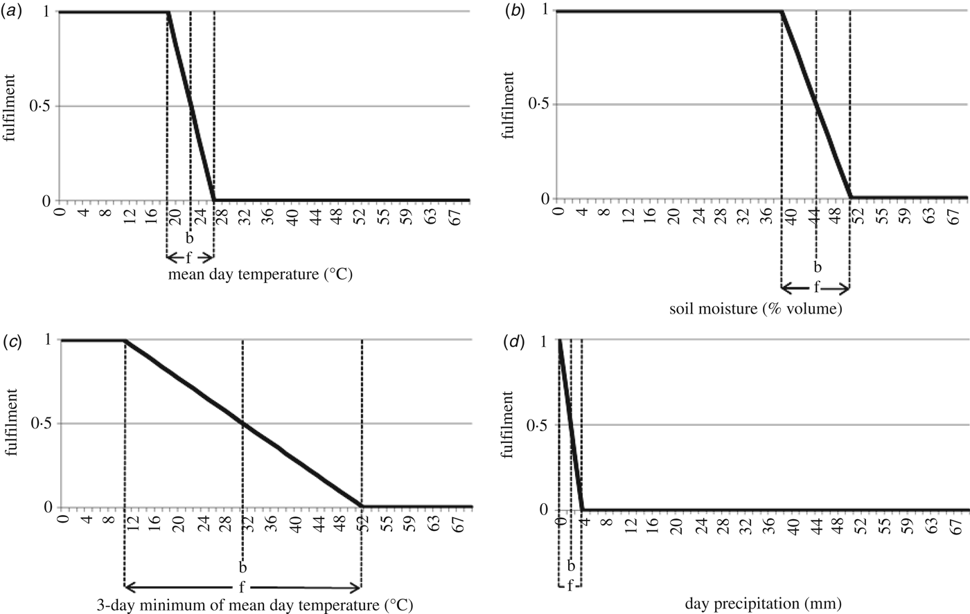
Each trigger is given a base value and a degree of ‘fuzziness’ stipulating the range where the fulfilment of the trigger gradually moves from 0 (impossible) to 1 (perfectly suitable) for an action (Fig. 2). A composite of all triggers is calculated each day and must exceed a given threshold (for the current work: 0·50 or ‘half-perfect’) for action. This composite t* is the geometric mean of the normalized fulfilment t of each fuzzy trigger k and is calculated as:
 $${t^{\ast}} = {[\Pi _{k = 0}^n \,{t_k}]^{1/n}}$$
Where t = [υ − (b − f/2)]/f for minimum triggers and t = [b + (f/2)−υ]/f for maximum triggers, n is the number of triggers, b is the minimum or maximum base value for each, f is its band of fuzziness (halved between greater and less than the base) and v is the currently simulated value. All ts are truncated to be between 0 and 1.
Membership functions of fuzzy triggers for the planting of winter wheat. (a) Maximum mean daily air temperature, (b) maximum soil moisture (c) maximum 3-day minimum of mean daily air temperature and (d) maximum total daily precipitation. b: Trigger base value, f: fuzziness of trigger (source: own depiction)
This was implemented in FarmActor at daily resolution using the programming language Java. It provides a clear interface to simulated behaviour, an entry point for experiments in actor profiles.
Model calibration
Calibration was conducted in three stages, starting with the base calibration of Expert-N to experimental field observations, followed by calibration of planting dates to phenological records and finally, building on accurate simulation of recent years, annual changes in crop model parameters were added.
Crop model calibration
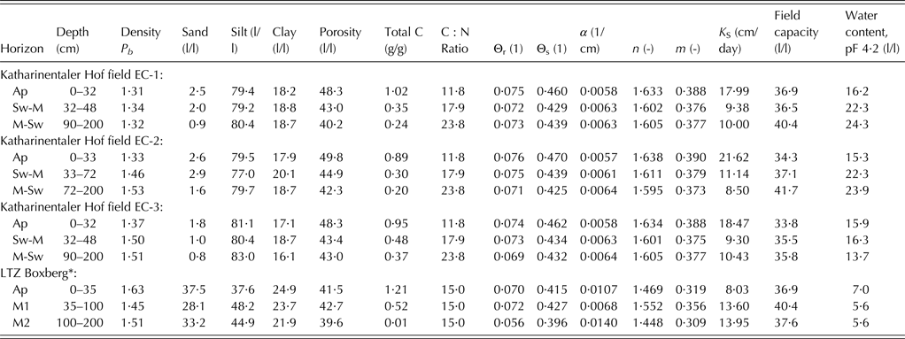
Two crop growth models, Genotype-by-Environment interaction on CROp growth Simulator (GECROS) and Crop Environment REsource Synthesis (CERES), were applied separately within Expert-N to provide a broader perspective on the effects of climate on crop performance. Both were calibrated using identical weather data, soil parameters and crop performance observations. See Table 3 for details of soil properties and hydraulic parameters.
Soil properties and hydraulic parameters
* LGRB reference profile DE6517-5 (LGRB 1997).
Both models were iteratively calibrated using UCODE (Poeter et al. Reference Poeter, Hill, Banta, Mehl and Christensen2005). Phenological parameters were optimized first and then, with these fixed, drivers of crop growth and yield formation were calibrated. Default parameters that were not adjusted are available for CERES in Priesack (Reference Priesack2006) and GECROS in Yin & Van Laar (Reference Yin and Van Laar2005).
Dynamic genetics
One of the latest capacities of crop modelling is accounting for the diversity of cultivars (Jeuffroy et al. Reference Jeuffroy, Casadebaig, Debaeke, Loyce and Meynard2014). While technological progress including the breeding of new crop cultivars has been credited with much of the yield increases in recent decades, allowing for this element has been elusive to crop modellers, leading to statistical correction of yields (Ewert et al. Reference Ewert, Rounsevell, Reginster, Metzger and Leemans2005). Further, simulating crop performance over a range of decades with static crop model parameters calibrated to specific years has resulted in failure to capture trends in crop yields and phenology (Aurbacher et al. Reference Aurbacher, Parker, Calberto Sánchez, Steinbach, Reinmuth, Ingwersen and Dabbert2013). Thus, one of the areas for improvement in crop modelling is a process-based way to account for the evolution of genotypes. To demonstrate how this can improve model accuracy, trends in some genetic parameters interpreted by the crop models were incorporated.
The genetic contribution to increased wheat and barley yields over recent decades has, through extensive cultivar trials, been largely attributed to grain number per ear (Ahlemeyer & Friedt Reference Ahlemeyer and Friedt2012) so that breeding has resulted in an increase of around 0·15 grains/ear/year between 1966 and 2007. However, Ahlemeyer & Friedt (Reference Ahlemeyer and Friedt2012) also showed complementary improvements in disease resistance as a result of breeding. Further, technological and climatic factors, including atmospheric CO2 fertilization, have contributed to yield trends (Lobell et al. Reference Lobell, Schlenker and Costa-Roberts2011). This precludes an exaggerated use of dynamic grain number to match observed historic yields.
Based on yield sensitivity, the initial leaf N content in GECROS was used to create a trend in simulated winter rapeseed yields. Another option would be to adjust thousand kernel weight, since its genetic advance has been well documented (Ali et al. Reference Ali, Javidfar, Elmira and Mirza2003; Marjanović-Jeromela et al. Reference Marjanović-Jeromela, Marinković, Ivanovska, Jankulovska, Mijić and Hristov2011).
Silage maize yields in Karlsruhe District show only a slight upward trend (+0·067 t/year) between 1981 and 2010. Phenological records at Oberderdingen however, show the start of local maize harvest trending later by 1·35 days/year. Bassu et al. (Reference Bassu, Brisson, Durand, Boote, Lizaso, Jones, Rosenzweig, Ruane, Adam, Baron, Basso, Biernath, Boogaard, Conijn, Corbeels, Deryng, De Sanctis, Gayler, Grassini, Hatfield, Hoek, Izaurralde, Jongschaap, Kemanian, Kersebaum, Kim, Kumar, Makowski, Müller, Nendel, Priesack, Pravia, Sau, Shcherbak, Tao, Teixeira, Timlin and Waha2014) propose that adaptation to greater cumulative temperatures in future growing seasons are likely to include the selection of later-ripening maize cultivars. This can be realistically achieved in simulations with an annual increase in the temperature requirement for the crop's juvenile stage, evidence for which has been established in German maize (Estrella et al. Reference Estrella, Sparks and Menzel2007).
Calibration of field management
Adaptive crop management in the face of global change could mean the difference between increasing and decreasing future yields, varying by crop (Leclère et al. Reference Leclère, Jayet and de Noblet-Ducoudré2013). To track historic climatic adaptation by local farmers and consequently project the same into the future, FarmActor conducts daily integration of Expert-N with database soil and weather records and internal management decision-making. Sensitivity analysis of simulated wheat yields produced by the coupled models during simulation years 2001–2010 showed a 370 kg/ha increase when planting a week earlier compared with a 121 kg/ha decrease when planting a week later than the average simulated planting date. Respective equivalents were: for winter barley, 47·8 and 1·0 kg/ha; spring barley, 114 and 142 kg/ha; oilseed rape, 342 and 449 kg/ha and silage maize, 131 and 323 kg/ha. FarmActor's dynamic crop rotation (Aurbacher & Dabbert Reference Aurbacher and Dabbert2011) was omitted to simplify the extraction of annual performance measures of each crop and to determine planting and harvest dates based on daily crop, soil and weather conditions, in addition to learning. Ten-year moving averages of soil temperature for spring crops and cumulative air temperature for winter crops were used to represent farmer learning from historic weather (Aurbacher et al. Reference Aurbacher, Parker, Calberto Sánchez, Steinbach, Reinmuth, Ingwersen and Dabbert2013). To accommodate the lack of crop rotation, soil nutrient values were reset each year.
The simulated farmer, in seeking to maximize crop yield and minimize risk, has an inevitably simplified set of criteria for each action, crop and field. Field-specific soil properties determine the moisture level corresponding to a favourable response to action, and that at which traffic and tillage can be withstood without the long-term damage of compaction (Rotz & Harrigan Reference Rotz and Harrigan2005). Recent and immediate weather determine soil moisture and are themselves direct criteria for action, varying with crop-specific temperature requirements.
Use of a genetic algorithm to calibrate management
The proper specification of action triggers is crucial for the functioning of the model. Although they are based in principle on expert knowledge, there remains a certain range of reasonable settings. The goal was to set the triggers such that the model optimally reproduced observed actions of farmers. To systematically apply the information from observations to trigger settings a genetic algorithm was used with a (μ + λ) evolutionary strategy, according to Schöneburg et al. (Reference Schöneburg, Heinzmann and Feddersen1994), where all former generations are retained.
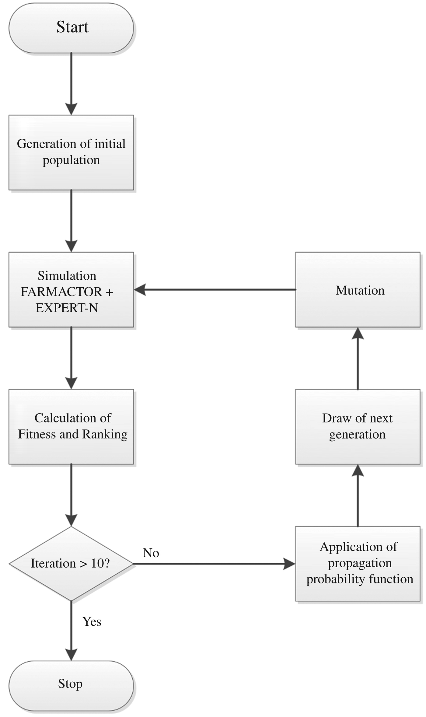
Functioning of the genetic algorithm proceeded as follows (see also Fig. 3): The first step was to define the possible range for each action-specific trigger based on agronomic principles. A population of potential values was created by assigning a number of intervals within the possible range to each trigger. The resultant population size was the product of the number of intervals of the different triggers. In the first iteration, the population was generated by choosing the centre of each interval within each trigger range (with one interval the value was at midpoint of the range, two intervals gave values at one and three quarters, three intervals at one-sixth, half and five-sixths, etc.). The model was then run for all population members and a fitness function evaluated upon completion. Root Mean Squared Error (RMSE) in days between observed and modelled action dates was used as the measure of fitness. Additionally, for every simulated year in which a combination of triggers resulted in a failed planting (by being too restrictive) a ‘penalty’ of 10 days was added to the RMSE to lead the algorithm away from that solution. The members of the population (trigger set) were then ranked according to fitness and if identical fitness values arose the rank was assigned randomly. The penalty ensured that population members with failed runs always ranked behind completely successful runs.
Schematic representation of genetic algorithm for calibration of management action triggers (source: own depiction).
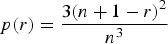
Next a propagation probability function was used to assign to each member of the population the likelihood that it would be one of the starting points of the following iteration. The function used was:
 $$p(r) = \displaystyle{{3{{(n + 1 - r)}^2}} \over {{n^3}}}$$
where p is the assigned probability, n is the size of the population and r is the rank of each population member (1 being the best, n the worst). This quadratic function assigned the probability 3/n to the first-ranked member (equal to a multiplication of the ‘fair chance’ 1/n by the factor 3) and the probability 3/n 3 (slightly larger than zero) to the one deemed of worst fitness. About 0·60 of the population members were assigned a value lower than fair chance while those remaining were privileged.
A new population of the same size was drawn from the preceding population using the assigned probabilities. Members of the new population were not exact copies of their ‘ancestors’, as ‘mutation’ occurred. Each trigger parameter was modified by adding a normally distributed random number with a pre-defined standard deviation. The standard deviation employed was reduced by the factor 0·9 in each successive iteration.
The model was re-run with the new generation of parameters, evaluated and successively propagated with respect to fitness rank. Members of previous iterations were not discarded but also included in the ranking and selection process of further iterations.
The parameter bounds, interval number and standard deviation used to find optimum values for each trigger were the same for winter wheat, barley and rapeseed, likewise for spring barley and maize. These values are given in Supplementary Table 1 (available from: http://journals.cambridge.org/AGS).
A drawback of this approach was the need to run the model repeatedly, resulting in a potentially long calibration time. To calibrate planting criteria, a population of 12 trigger sets was run for ten iterations from 1981–2010 for winter wheat, winter rapeseed and maize, establishing learning (expectations) for the first 10 years and comparing simulated planting dates during 1991–2010 to phenological observations at Oberderdingen. This left the years 1981–1990 at Oberderdingen available for validation of simulated planting of these crops. Summer and winter barley were likewise run from 1971–1990, calibrating to the latest available phenological observations at Oberderdingen and Helmstadt, respectively, while validation for spring barley depended on state field trial records.
RESULTS AND DISCUSSION
Crop model calibration results
Within Expert-N, GECROS was, for all crops, calibrated to a greater degree of Nash & Sutcliffe (Reference Nash and Sutcliffe1970) model efficiency than CERES, though yield accuracy (by RMSE) was better with CERES for winter wheat and winter barley, but better with GECROS for spring barley and silage maize. Both models attained the poorest fit with silage maize, the best with summer barley and wheat in between, keeping in mind the less comprehensive data for barley. Final sets of parameters and model fit after calibration of GECROS and CERES are given in the Supplementary Material (Supplementary Tables 2 and 3, respectively, available from: http://journals.cambridge.org/AGS).
Calibrated dynamic genetics
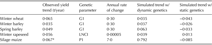
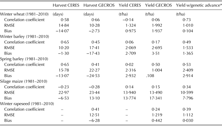
Based on measurements for wheat by Ahlemeyer & Friedt (Reference Ahlemeyer and Friedt2012) and resolved to field measurements of combined stem and ear weight of 4·4 g DW/plant and 2·2 ears/plant (0·5 ears/g) (Högy & Fangmeier Reference Högy, Fangmeier and Hoffman2013), the CERES parameter for the number of grains/g of stem (G2) was adjusted by 0·3 each year relative to the calibrated values, decreasing before and increasing after 2010. This effect was also applied to winter and spring barley. The initial leaf N content of rapeseed (LNCI) was likewise set to change by 0·14% each year to better approximate the observed yield trend. The thermal requirement for the juvenile stage of maize (P1) was adjusted to improve model fit of simulated to observed harvest dates. This increased the 1981–2010 maize yield trend from less than to more than that of district averages. However, the new trend is still less than that observed at state cultivar trial stations during 1990–2010 (LTZ Augustenberg 2013). In winter wheat and rapeseed, simulated yield trends were a portion of that observed, while in both barley crops the chosen settings over-compensated for genetic advance. Table 4 shows the observed yield trends in the district, values for genetic advance used in simulation and the resultant simulated trends (sensitivity analysis results at the chosen rates of genetic change are not presented here but are available from the authors upon request).
Observed Karlsruhe Rural District yield trends, simulated genetic advance and yield trends with and without dynamic genetics, 1981–2010
G1, grains/g stem; LNCI, initial leaf nitrogen [g N/g]; P1, cumulative temperature (base 8 °C) from emergence to end of juvenile stage
* In comparison, the yield trend from state trials, across all cultivars being tested in the Kraichgau, 1990–2010, was 1·072 t/year (LTZ Augustenberg 2013).
While integrating genetic advance shows promise, extensive calibration to match historic yields was not undertaken, considering that other technological factors surrounding pest control, fertilization and farm management have played a significant role in recently increasing yields (Friedt & Ordon Reference Friedt, Ordon, Zhang, Li and Liu2013). Further work should use additional experimental data and more extensive calibration to isolate those genotype parameters in both CERES and GECROS that are best used to account for breeding progress.
Management calibration results
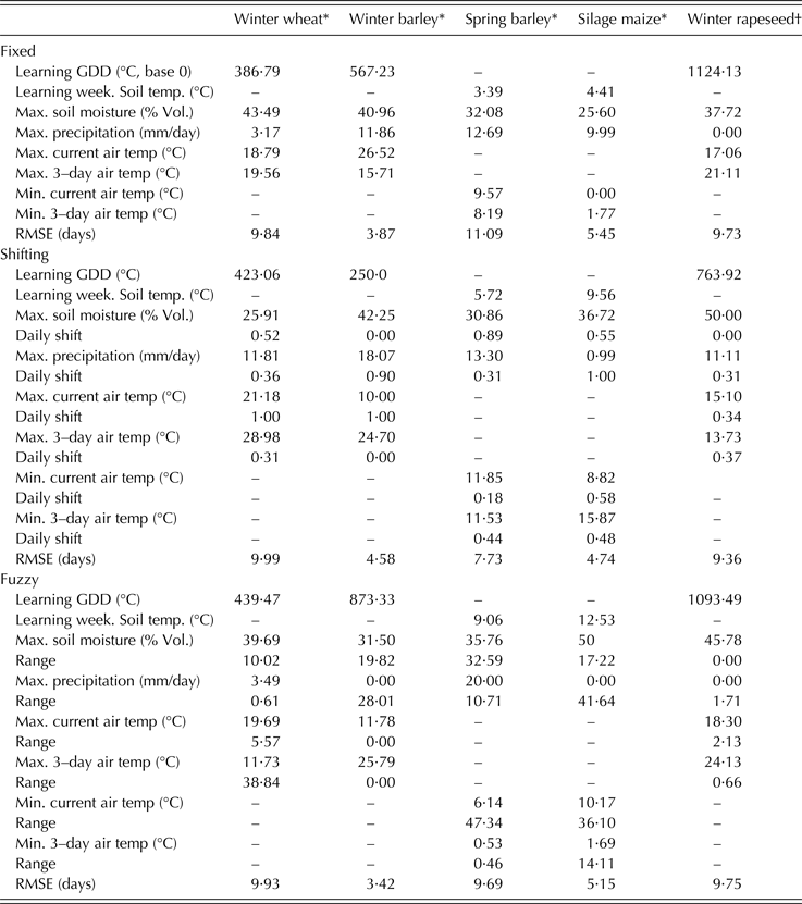
In calibrating spring planting dates, shifting trigger values consistently produced the most accurate predictions, followed by fuzzy and then fixed/override triggers. Autumn planting was not as decisive, with each of the three paradigms resulting in the best predictions for one crop. Table 5 has results of calibration with the genetic algorithm for the different behavioural paradigms. The best target value is given along with its corresponding set of trigger values.
Optimized planting trigger values and fit (RMSE) for planting of different crops
* Modelled with CERES for planting calibration.
† Modelled with GECROS for planting calibration.
Model validation
Validation of simulated planting dates compares model output with DWD network observations outside of the calibration period. Outcomes determine which trigger paradigm and how changing genetics were used in later projections.
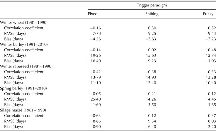
The model was run for the five crops from 1970–2010 (the first 10 years of temperatures needed as a warm-up phase for learning) with ‘fixed’, ‘shifting’ and ‘fuzzy’ action triggers to compare them by RMSE, correlation coefficient and bias.
Spring planting dates during the validation period were consistently predicted more accurately using fuzzy triggers, followed by shifting and then fixed/override. Simulation of autumn planting did not benefit so clearly from the more complicated paradigms, but a trade-off between accuracy measures leaves evaluation open to judgment (Table 6). It was decided to proceed with fuzzy triggers with all five crops in validation of harvest results and forthcoming projections.
Validation period measures of fit for simulated planting dates by crop and action trigger paradigms
Harvest date and yield validation is possible during the entire 1981–2010 simulation period using DWD records of harvest date and district average yields. Evident in the results is that simulated crop yields from both CERES and GECROS consistently exceeded those observed in the area as Karlsruhe rural district averages (see Table 7 yield biases). This, however, should be expected when comparing regional averages, irrespective of farm type, to simulations based on data from more optimally managed, highly productive fields, as is the case both at Katherinentaler Hof and state field trial stations. Incorporating dynamic genetics into the model reduces yield bias, as well as the other measures of model fit (Table 7) which also shows that simulated maize phenological development was slightly more accurate with CERES, while yields were more accurately reproduced with GECROS. Validation measures are comparable with that from other studies that generally involve shorter periods. Rötter et al. (Reference Rötter, Palosuo, Kersebaum, Angulo, Bindi, Ewert, Ferrise, Hlavinka, Moriondo, Nendel, Olesen, Patil, Ruget, Takáč and Trnka2012) showed nine different crop models simulating spring barley at seven sites in Europe over a maximum of 14 years with yield RMSE between 1 and 2 t/ha. In a similar study Palosuo et al. (Reference Palosuo, Kersebaum, Angulo, Hlavinka, Moriondo, Olesen, Patil, Ruget, Rumbaur, Takáč, Trnka, Bindi, Çaldağ, Ewert, Ferrise, Mirschel, Şaylan, Šiška and Rötter2011) modelled winter wheat with eight crop models at eight sites over a maximum of 14 years and reported the lowest yield RMSE to be 1·43 t/ha. Mast et al. (Reference Mast, Claupein and Graeff-Hönninger2014) simulated maize dry matter production, also in Southwest Germany, with a RMSE over 5 years of 9 t/ha; Angulo et al. (Reference Angulo, Rötter, Lock, Enders, Fronzek and Ewert2013) with the most complex of three calibration strategies in their study simulating winter wheat and winter barley over 24 years achieved yield RMSE between 0·6 and 0·7 t/ha. In contrast to the above studies, simultaneous simulation of planting and harvest dates, rather than using observations, added to the scope of cropping simulations but detracted from the accuracy of replicating historic yields.
Validation period measures of fit for simulated harvest dates and yield by crop and model
* Wheat, barley and maize with CERES, rapeseed with GECROS.
Satisfactory validation supports the following projections of Kraichgau agriculture in the coming decades. Climate forcing of field management and crop performance utilized WETTREG 2010 simulated future weather scenarios (Kreienkamp et al. Reference Kreienkamp, Enke and Spekat2010) for the Eppingen station, based on its historic records and assuming IPCC scenario A1B (IPCC Core Writing Team et al. Reference Pachauri and Reisinger2007).
Projections
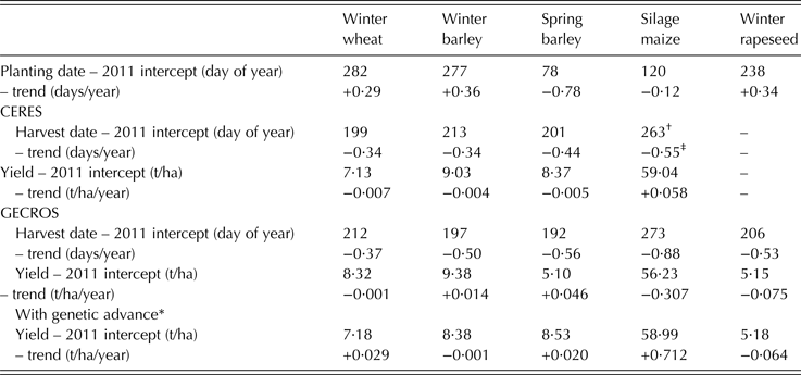
Projections were made for the 30 years after the base year 2010. Three runs were performed using separate realizations (ID# 2500200, 2500244 and 2500288) of the same WETTREG scenario at Eppingen. Regression function intercept and slope for planting, harvest and yield, averaged from the three runs are presented in Table 8.
Projected management and crop performance statistics 2011–2040
* Wheat, barley and maize with CERES, rapeseed with GECROS.
† w/changing genetics = 260·04.
‡ w/changing genetics = +0·96.
Based on integration of simulated weather, soil conditions and farmer behaviour, the model indicated that winter crops will be sown about 1 day later for every 3 years into the future, in a warming climate, while still receiving the appropriate cumulative temperature for pre-vernalization development and satisfying other agronomic restrictions. Sowing of malting barley in the spring would change faster, 1 day earlier every 2 years based on CERES crop growth and concomitant soil conditions, and even faster according to GECROS-based simulations. Planting of maize would not be adapted as quickly, but would still shift to earlier dates.
The warmer temperatures in simulated future weather drove harvest dates earlier in all crops, 1 day per 3 years in winter wheat. Barley and rapeseed harvest dates were projected to be earlier by around 1 day every 2 years. Harvest of silage maize occurred >1 day earlier every 2 years according to CERES, nearer to 1 day per year using GECROS. Using dynamic genetics reversed this trend so that maize was harvested 1 day later each year.
Both crop models with static genetics projected yields of winter wheat to trend very slightly downward over the next 30 years. However, the increasing harvest index programmed as CERES input made for an increase in wheat productivity. CERES barley showed slightly declining yields with static genetics but an improved outlook with dynamic crop model parameters. GECROS projects slight and moderate increase in winter and spring barley, respectively. Maize yields using CERES were projected to increase slightly in the future, while with GECROS the trend is negative, with numerous poor crop yields, resulting from simulated soil moisture being near the permanent wilting point over extended periods during the summer. Continuing the shift in one rapeseed physiological parameter with GECROS reduced the simulated negative impact of global change on seed yield. In either case, winter rapeseed appeared to become the most negatively affected of the region's five major crops.
CONCLUSIONS
The current study presents an outlook on farm management and crop performance specific to the Kraichgau into the coming decades. Results show that cereal productivity may remain steady even under global climate change. The situation for maize and rapeseed is not, however, so evident. The two crop growth models produce contrasting results; with CERES maize yields appear to increase, while, due to greater sensitivity to drought, GECROS produces a declining yield trend. Rapeseed simulation with GECROS indicates that declining seed yields through 2040 could dampen or even reverse the current increase in rapeseed cultivation in the area (DESTATIS 2014). Yield declining due to climate change could be partially offset by breeding progress and increasing atmospheric carbon dioxide, but exacerbated by pest and disease prevalence; however these factors beg confirmation with more extensive modelling.
Aurbacher et al. (Reference Aurbacher, Parker, Calberto Sánchez, Steinbach, Reinmuth, Ingwersen and Dabbert2013), modelling the nearby mountainous Swabian Alb, projected more drastic negative trends in wheat and maize yields, albeit with less extensive crop model calibration and no genetic dynamics. Angulo et al. (Reference Angulo, Rötter, Lock, Enders, Fronzek and Ewert2013) projected decreasing yields for five major European crops, based solely on climate change. However, when technological change and CO2 fertilization are included projections become more optimistic.
While the simulated future growing season, e.g. time between spring and autumn frosts, is expanding, warmer temperatures ripen crops faster so that farmers should choose later-ripening cultivars to profit from the extended season. Alternatively, the simultaneous trends toward earlier harvest and later (autumn) planting may affect future crop rotations. For example, by 2040, at base temperatures 0 °C (e.g. wheat) and 8 °C (maize) according to the average of the three future weather realizations there will be around 2200 and 1200 GDD, respectively, available for plant development between 1 July and 1 November (Kreienkamp et al. Reference Kreienkamp, Enke and Spekat2010), sufficient for a complete life cycle of a second crop (Deryng et al. Reference Deryng, Sacks, Barford and Ramankutty2011). As proposed in Waha et al. (Reference Waha, Müller, Bondeau, Dietrich, Kurukulasuriya, Heinke and Lotze-Campen2013), mitigation of climatic risks may well include such double cropping.
The use of simulated future weather in conjunction with flexible management accounts for some of the adaptation that should be expected from farmers under changing climate. Fuzzy logic is a promising way of depicting the decision-making process behind field management, adding credence to the timing of actions in bio-economic models which have a clear influence on results. This should improve both the accuracy of measures such as yields and offers further statements on alternative cropping practices, like double cropping. The adaptability of cultivar selection is another factor that contributes to model plausibility, as the attributes of available varieties change over time and through their use, alter the context of field cropping.
The latest extensions to FarmActor further extricate its subject, the simulated farmer and field, from the limitations of an agro-economic constellation in favour of an adaptive system evolving through time. Future work may include implementation of climate projections produced with coupled atmosphere-land surface models to allow inclusion of feedback between land-use changes and regional climate. Planting trigger calibration would benefit from more extensive calibration, and application of fuzzy logic into other actions (harvest, tillage, fertilization, etc.) may follow. Also, incorporation of CO2 fertilization, crop pests, frost damage, plus further specification of changing crop genetics should add to overall robustness.
The supplementary material for this article can be found at http://www.journals.cambridge.org/AGS
The authors gratefully acknowledge funding from the German Research Foundation (Deutsche Forschungsgemeinschaft, DFG) under the grant FOR1695, and also the owners of experimental fields for permission to use management records and take measurements. Further thanks are due to Sebastian Gayler and German A. Calberto Sanchez for their technical assistance with crop model calibration.