INTRODUCTION
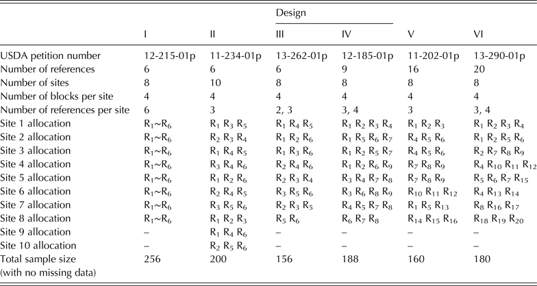
Safety evaluation of a genetically modified (GM) crop entails establishing its substantial equivalence to conventional non-GM food crops with respect to key agronomic, phenotypic and compositional endpoints (OECD 1993; Codex Alimentarius Commission 2009). The European Food Safety Authority (EFSA) mandates a comparative analysis containing two types of statistical tests (EFSA 2010). For each endpoint, a difference test is used to detect the potential change in the genetically modified organism (GMO) from its non-GM counterpart (control) whereas an equivalence test is used to assess GMO's similarity to commercial non-GM reference varieties with a history of safe use. Studies on GMO safety include multiple sites and within each site, a GMO is planted together with its control and several non-GM reference varieties according to a randomized complete block design. Features of the design are determined by the arrangement of references to sites. Table 1 reports designs implemented in recent petitions by ag-biotech producers to the US Department of Agriculture (USDA): Design I is complete and balanced; Design II is incomplete but balanced; Designs III–VI are incomplete and, following the descriptions in Section 1.2 of Searle (Reference Searle1987), are ‘planned unbalanced’.
Field designs implemented for GMO safety evaluation (information available online from http://www.aphis.usda.gov/biotechnology/petitions_table_pending.shtml (verified 3 December 2015))
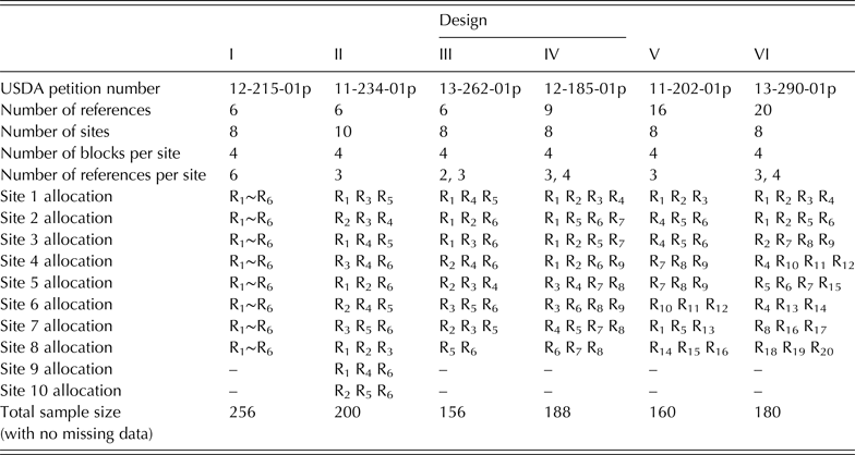
GMO, genetically modified organism; USDA, US department of agriculture.
Compositional data usually undergoes a natural logarithm transformation before the mixed model analysis. Let n R be the total number of references in the study. Let n S and n B(S) be the number of sites and number of blocks per site. Denote Y ijl as the log-transformed response with respect to a given endpoint from genotype i in block l at site j, i = 1, …, n R + 2, j = 1, …, n S, l = 1, …, n B(S). Note that Y ijl is observed only when genotype i is present at site j; otherwise, it is unavailable. The EFSA (2010) and Van der Voet et al. (Reference Van der Voet, Perry, Amzal and Paoletti2011) conducted the comparative analysis under the following linear mixed model which accommodates the effect of the n R + 2 genotypes in a hierarchical structure with both fixed and random levels.
 $$Y_{{\rm ijl}} = \left\{ {\matrix{ {\mu _{\rm R} + S_{\rm j} + B(S)_{{\rm l(\,j)}} + R_{\rm i} + E_{{\rm ijl}} \quad \;\quad i = 1,...,n_{\rm R} \;\quad} \cr {\mu _{\rm T} + S_{\rm j} + B(S)_{{\rm l(\,j)}} + E_{{\rm ijl}} \quad \quad \quad \quad i = n_{\rm R} + 1\quad \quad} \cr {\mu _{\rm C} + S_{\rm j} + B(S)_{{\rm l(\,j)}} + E_{{\rm ijl}} \quad \quad \quad \quad i = n_{\rm R} + 2\quad \quad} \cr}} \right.$$
Fixed effects of the three genotype groups, namely, reference, GMO (test product) and control, are represented, respectively, by μ
R, μ
T and μ
C. Because individual producers select their own assortment of reference varieties for each study, the deviation of the mean of reference genotype i from its group mean μ
R is modelled by the random effect R
i which is normally distributed with mean zero and variance
 $\sigma _{\rm R}^2 $
, i.e.
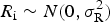 $R_{\rm i} \sim N(0,\sigma _{\rm R}^2 )$
. Random effects of site and block nested within site are represented, respectively, by
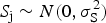 $S_{\rm j} \sim N(0,\sigma _{\rm S}^2 )$
and
 $B(S)_{{\rm l}({\rm j})} \sim N(0,\sigma _{{\rm B}({\rm S})}^2 )$
. The error term
 $E_{{\rm ijl}} \sim N(0,\sigma _{\rm E}^2 )$
combines random effects due to plot, measurement uncertainty and other sources of unexplained variation. All random terms are jointly independent. The EFSA (2010) described the comparative analysis as ‘mainly concerned with studying the average difference and the average equivalence over sites’ and chose to ‘set a lower and upper equivalence limit based on the variability observed among the commercial varieties’. Its current guidance tests the average equivalence with data-driven equivalence limits (ELs), i.e.
 $$\eqalign{& H_0 :\mu _{\rm T} - \mu _{\rm R} \les - \hat PL\;\;or\;\;\mu _{\rm T} - \mu _{\rm R} \ges \hat PL\quad v. \cr & H_1 : - \hat PL \lt \mu _{\rm T} - \mu _{\rm R} \lt \hat PL,} $$
where (
 $ - \hat PL$
,
 $\hat PL$
) corresponds to a version of the 95% prediction interval of R
i estimated concurrently under Model (1). Upon treating these two prediction limits as known 2·5th and 97·5th percentiles of
 $N(0,\sigma _{\rm R}^2 )$
, the traditional two one-sided tests (Schuirmann Reference Schuirmann1987) were employed. Unfortunately, judging μ
T − μ
R against estimated ELs is fraught with problems, foremost of which is that statistical hypotheses should always be defined in terms of model parameters rather than their estimators; otherwise, the type I error rate is intractable. In addition,
 $\hat PL$
decreases as sample sizes increase. This unfairly imposes smaller and, hence, more stringent ELs on studies with larger sample sizes. A thorough discussion on the pitfalls of Hypotheses (2) can be found in Appendix 3 of Vahl & Kang (Reference Vahl and Kang2015).
The average equivalence specified by EFSA (2010) was expressed explicitly in terms of model parameters by Kang & Vahl (Reference Kang and Vahl2014) as
 $$\eqalign{& H_0 :\mu _{\rm T} - \mu _{\rm R} \les - z_{0{\cdot}975} \sigma _{\rm R} \;\;or\;\;\mu _{\rm T} - \mu _{\rm R} \ges z_{0{\cdot}975} \sigma _{\rm R} \quad v. \cr & H_1 : - z_{0{\cdot}975} \sigma _{\rm R} \lt \mu _{\rm T} - \mu _{\rm R} \lt z_{0{\cdot}975} \sigma _{\rm R}} $$
where z
0·75 is the 97·5th percentile of a standard normal distribution (Note: z
0·025 = −z
0·975). Hypotheses (3) assess the mean difference of the test and reference products based on
 $\sigma _{\rm R}^2 $
, the variability of the super-distribution of reference genotype means. Vahl & Kang (Reference Vahl and Kang2015) referred to it as addressing ‘super-equivalence’. Tuning the EL according to σ
R is reasonable when
 $\sigma _{\rm R}^2 $
dominates the reference natural variation. For endpoints with a small observed value of
 $\sigma _{\rm R}^2 $
, EFSA (2010) recognized that their
 $\hat PL$
s lack biological relevance and excluded these endpoints from equivalence testing. With similar concern, Vahl & Kang (Reference Vahl and Kang2015) identified ‘conditional equivalence’ as a reasonable alternative to super-equivalence. This new class of equivalence compares measurements from field plots planted with GMO to those with references according to their conditional distributions at the site and block level. Depending on one's preference, conditional equivalence can be defined in two forms: the conditional scaled average equivalence (SAE-C) and the conditional distribution-wise equivalence (DWE-C). A unified expression for hypotheses of conditional equivalence is
 $$\eqalign{& H_0 :\mu _{\rm T} - \mu _{\rm R} \les - \sqrt {z_{0{\cdot}975}^2 \sigma _{\rm R}^{\rm 2} + c\sigma _{\rm E}^2} \quad or \cr & \mu _{\rm T} - \mu _{\rm R} \ges \sqrt {z_{0{\cdot}975}^2 \sigma _{\rm R}^2 + c\sigma _{\rm E}^2} \quad v. \cr & H_1 : - \sqrt {z_{0{\cdot}975}^2 \sigma _{\rm R}^2 + c\sigma _{\rm E}^2} \lt \mu _{\rm T} - \mu _{\rm R} \lt \sqrt {z_{0{\cdot}975}^2 \sigma _{\rm R}^2 + c\sigma _{\rm E}^2}} $$
Setting
 $c = z_{0 \cdot 975}^2 $
gives rise to SAE-C, which requires the GMO mean to fall within 2·5th and 97·5th percentiles of the reference distribution at the site and block level. Testing SAE-C stems from the routinely implemented strategy for statistical quality control where the test product is required to provide values falling within a certain percentage of the reference distribution. It also harmonizes with the current assessment of highly variable drugs via its rescaled average bioequivalence at the individual subject level (Davit et al.
Reference Davit, Chen, Conner, Haidar, Kim, Lee, Lionberger, Maklouf, Nwakama, Patel, Schuirmann and Yu2012). Setting
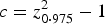 $c = z_{0 \cdot 975}^2 - 1$
originates from the well-established statistical principle of controlling the information divergence between conditional distributions (for its connection to individual bioequivalence see Dragalin et al.
Reference Dragalin, Fedorov, Patterson and Jones2003). The corresponding notion of DWE-C is more stringent than SAE-C but maintains its meaning for any monotonically transformed data. This is particularly appealing for assessing GMO agronomic-phenotypic characteristics. However, DWE-C has been deemed too mathematical, at least for drug studies (see Vahl & Kang Reference Vahl and Kang2015 for more discussions on this issue). In spite of the conceptual connection between GMO conditional equivalence and drug bioequivalence, it must be noted that drug bioavailability studies differ remarkably from GMO safety studies with respect to purpose, experimental design and model. In vivo drug bioavailability studies intend to assess the difference between a test drug and a single reference product via a crossover design. Their statistical analyses employ typical mixed models where both levels of the treatment effect are fixed. Safety studies for GMOs include an assortment of non-GM commercial reference varieties to assess GMO in the context of natural variation. Data collected in multi-site randomized block field trials are usually unbalanced and incomplete, by design or execution. Model (1) is atypical because genotype contains both fixed and random levels. In contrast to the U S Food and Drug Administration's recent recommendation of SAE-C as a usable bioequivalence criterion (FDA 2014), there has been no regulatory clarification on the explicit definition of GMO equivalence. It is therefore prudent to create statistical testing procedures that establish both SAE-C and DWE-C.
Statistical methodologies for inference on functions of means and variances have been investigated mostly within the context of testing bioequivalence in drug studies and estimating tolerance intervals for monitoring purposes. Two methods have been commonly employed there: the modified-large-sample (MLS) approximation (Howe Reference Howe1974; Graybill & Wang Reference Graybill and Wang1980; Hyslop et al. Reference Hyslop, Hsuan and Holder2000; Krishnamoorthy & Lian Reference Krishnamoorthy and Lian2012) and a method via generalized pivotal quantities (GPQs) (Tsui & Weerahandi Reference Tsui and Weerahandi1989; Weerahandi Reference Weerahandi1993; McNally et al. Reference McNally, Iyer and Mathew2003; Krishnamoorthy & Mathew Reference Krishnamoorthy and Mathew2004; Liao et al. Reference Liao, Lin and Iyer2005; Hannig et al. Reference Hannig, Iyer and Patterson2006; Chiu et al. Reference Chiu, Tsai and Liu2010). Both the MLS and GPQ methods call for exact distributions of independent summary statistics which are established results of linear model theory under balanced designs. As stated on p. 141 of Krishnamoorthy & Mathew (Reference Krishnamoorthy and Mathew2009), ‘for general mixed effects or random effect models with unbalanced data, a unified methodology is currently not available’. Krishnamoorthy & Mathew (Reference Krishnamoorthy and Mathew2004) as well as Krishnamoorthy & Lian (Reference Krishnamoorthy and Lian2012) conquered the problem of unbalanced data in a one-way random effect model by building moments around unweighted means; however their approach is unfeasible in Model (1), a three-way mixed model where the site effect crosses with the reference effect, due to missing combinations of site and reference (Section 4.6 of Searle Reference Searle1987). In addition, the model under clinical crossover designs contains correlated heterogeneous variance components, which are issues specific to drug bioequivalence studies. Clearly the unique characteristics of GMO testing require these statistical methods be derived from the ground up. Because the distribution of a GPQ generally depends on nuisance parameters, it is crucial to validate the GPQ method when venturing into a new application. This also pertains to the MLS approximation. To date, only Hypotheses (3) have received careful attention and this was accomplished exclusively via the GPQ method (Kang & Vahl Reference Kang and Vahl2014).
The purpose of the present work is to develop and validate statistical procedures for testing Hypotheses (4) under Model (1). Special effort is made to tackle the incompleteness and unbalanced nature of field designs. The approach here is novel, in that it builds moments with tractable distributions under Model (1) based on the method of Khuri et al. (Reference Khuri, Mathew and Sinha1998). The practical appeal is manifest in the convenience of obtaining the required summary statistics output by standard statistical software rather than from custom programs carrying out tedious algebraic calculations. The Materials and Methods section introduces summary statistics especially useful for estimating parameters in Model (1). Their statistical properties, including distributions and dependencies, are established under a general setting. Accordingly, the present paper creates the statistical procedures for testing Hypotheses (4) via both the MLS and GPQ methods. The Results section investigates these newly proposed procedures via two sets of simulation studies. First, the small-sample behaviours of the MLS and GPQ procedures are inspected over an array of idealistic situations where the design is complete and balanced. Second, their performance is examined under practical designs listed in Table 1 with and without data randomly missing. The utility of these two procedures is also illustrated in a case study using summary statistics derived from a real-world data set. The last section of this paper makes additional comments on GMO equivalence testing.
MATERIALS AND METHODS
Properties of summary statistics
Because studies on GMO safety include a limited number of reference varieties, variance components tend to be overestimated by the restricted maximum likelihood (REML) method (Endrenyi et al. Reference Endrenyi, Taback and Tothfalusi2000; Park & Burdick Reference Park and Burdick2003). To avoid estimation bias, the method of moments was used in the current paper to estimate variances. Table 2 provides the analysis of variance (ANOVA) shell for complete and balanced designs under Model (1). Constructing the ANOVA tables and deriving weighted means under other designs involved tedious algebraic calculation. Nonetheless, these computed results were easily accessible via routine procedures of standard statistical software such as PROC MIXED in SAS (SAS Institute Inc. 2011).
ANOVA table for random effects in Model (1) under complete balanced designs

ANOVA, analysis of variance.
Khuri et al. (Reference Khuri, Mathew and Sinha1998, Section 4.3) extended the method of moments to general two-way random effect models. Their approach offers a viable solution for inferring variance components from unbalanced GMO field designs where not all combinations of site and references are present. Let
 ${\bf \sigma} ^2 $
be the vector of variance components in Model (1). The mean square for each random effect corresponds to a quadratic form whose expectation is a linear combination of elements in
 ${\bf \sigma} ^2 $
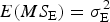
. Distributions of these mean squares were obtained directly from the application of classical mixed model theory. In particular, the mean square error MS
E has an expected value of
 $\sigma _E^2 $
, i.e.
 $E(MS_{\rm E} ) = \sigma _{\rm E}^2 $
, and follows a scaled χ
2 distribution with degrees of freedom (d.f.) df
E, i.e.
 $$\displaystyle{{df_{\rm E}} \over {E(MS_{\rm E} )}}MS_{\rm E} \equiv U_{\rm E} \sim\chi ^2 (df_{\rm E} )$$
The value of df
E is the rank of the quadratic matrix for MS
E. The mean square for the random effect of reference genotypes, denoted by MS
R has an expected value of
 $E(MS_{\rm R} ) = a\sigma _{\rm R}^2 + \sigma _{\rm E}^2 $
. Coefficient a > 0 is determined entirely by the design matrix. It attains the simple formulation of a = n
S
n
B(S) for complete and balanced designs (see Table 2). By construction, MS
R is independent of MS
E. The quadratic matrix of MS
R is of rank (n
R−1). The distribution of MS
R is, in general, represented by a weighted sum of (n
R−1) independent χ
2(1) random variables. When reference varieties are allocated to sites in a balanced fashion, as in Designs I and II, the weights all equal one so that the distribution of MS
R simplifies to a scaled χ
2(n
R−1) distribution. For unbalanced Designs III–VI, the distribution of MS
R was approximated by
 $$\displaystyle{{df_{\rm R}} \over {E(MS_{\rm R} )}}MS_{\rm R} \equiv U_{\rm R} \dot \sim\chi ^2 (df_{\rm R} )$$
with df R = n R − 1. Subsequent simulation studies indicated that equivalence tests based on this approximation perform reasonably well.
Denote the least square mean for μ
T − μ
R by
 $\bar D$
. By construction,
 $\bar D$
is independent of MS
R and MS
E. It is well-known that
 $$\displaystyle{{\bar D - \mu _{\rm T} + \mu _{\rm R}} \over {\sqrt {Var(\bar D)}}} \equiv Z\sim N(0,1)$$
The variance of
 $\bar D$
depends on the design matrix and
 ${\bf \sigma} ^2$
. Plug the point estimator of
 ${\bf \sigma} ^2$
into
 $Var(\bar D)$
. The resulting estimator,
 $\hat Var(\bar D)$
, is independent of
 $\bar D$
and approximately follows a scaled χ
2 distribution. That is,
 $$\displaystyle{{df_{\rm D} ({\bf \sigma} ^2 )} \over {Var(\bar D)}}\hat Var(\bar D)\dot \sim\chi ^2 (df_{\rm D} ({\bf \sigma} ^2 ))$$
where
 $df_{\rm D} ({\bf \sigma} ^2 )$
, as a function of
 ${\bf \sigma} ^2 $
, is the Satterthwaite approximation to the d.f. Also note that
 ${\rm Var}(\bar D)$
could be expressed as a linear combination of E(MS
R) and E(MS
E) with linear coefficient functions
 $h_1 ({\bf \sigma} ^2 )$
and
 $h_2 ({\bf \sigma} ^2 )$
, i.e.
 $Var(\bar D) = h_1 ({\bf \sigma} ^2 ){\rm E}(MS_{\rm R} ) + h_2 ({\bf \sigma} ^2 )E(MS_{\rm E} )$
. In balanced designs containing v references per site,
 $h_1 ({\bf \sigma} ^2 )$
and
 $h_2 ({\bf \sigma} ^2 )$
are constants with values
 $h_1 ({\bf \sigma} ^2 ) = (an_{\rm R} )^{ - 1} $
,
 $h_2 ({\bf \sigma} ^2 ) = (n_{\rm S} n_{{\rm B}({\rm S})} )^{ - 1} +(vn_{\rm S} n_{{\rm B}({\rm S})} )^{ - 1} $
 $- (an_{\rm R} )^{ - 1} $
. The distribution of
 $\bar D$
under these designs was then parameterized by E(MS
R) and E(MS
E) instead of
 ${\bf \sigma} ^2 $
.
Modified large sample method
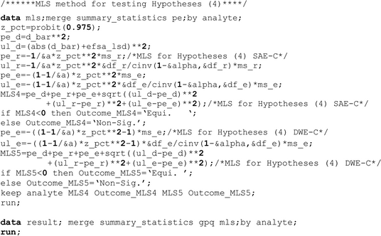
The MLS method was originally developed to approximate linear combinations of variances (Howe Reference Howe1974; Graybill & Wang Reference Graybill and Wang1980). Hyslop et al. (Reference Hyslop, Hsuan and Holder2000) extended the MLS method to assess drug bioequivalence by restating its hypotheses in terms of a linear combination of squared mean differences and variances. The present work adopted their strategy and rejected H
0 of Hypotheses (4) at the α significance level if the 100(1 − α)% MLS upper confidence limit (CL) for
 $(\mu _{\rm T} - \mu _{\rm R} )^2 - (z_{0 \cdot 975}^2 \sigma _{\rm R}^2 + c\sigma _{\rm E}^2 )$
was less than zero. In order to utilize the sampling distributions of the summary statistics, the following reparameterization was introduced.
 $$\eqalign{&(\mu _{\rm T} - \mu _{\rm R} )^2 - (z_{0{\cdot}975}^2 \sigma_{\rm R}^2 + c\sigma _{\rm E}^2 ) \cr & \qquad = (\mu _{\rm T} - \mu _{\rm R} )^2 \cr & \qquad - \displaystyle{1 \over a}z_{0{\cdot}975}^2 E(MS_{\rm R} ) - \left( {c - \displaystyle{1 \over a}z_{0{\cdot}975}^2} \right)E(MS_{\rm E} )}$$
Suppose that
 ${\bar d}$
, ms
R and ms
E are the respective observed values of
 $\bar D$
, MS
R and MS
E. Let PE
k and UL
k, k = D, R, E, be the point estimate and 100(1 − α)% upper CL for (μ
T − μ
R)2,
 $ - ({1 / a})z_{0 \cdot 975}^2 E(MS_{\rm R} )$
and
 $ - (c - z_{0 \cdot 975}^2 /a)E(MS_{\rm E} )$
, respectively. Properties (5)–(8) suggest that
 $$\eqalign{& PE_{\rm D} = {\bar d}^2, \cr & UL_{\rm D} = \{ \vert {\bar d} \vert + t_{1 - \alpha} (df_{\rm D} ({\hat {\bf \sigma}}^2 ))\sqrt {{\hat V}ar(\bar D)} \}^2 \cr & PE_{\rm R} = - \displaystyle{1 \over a}z_{0{\cdot}975}^2 ms_{\rm R}, \cr & UL_{\rm R} = - \displaystyle{1 \over a}z_{0{\cdot}975}^2 \displaystyle{{df_{\rm R} ms_{\rm R}} \over {\chi_{1 - \alpha}^2 (df_{\rm R})}} \cr & PE_{\rm E} = - \left( {c - \displaystyle{1 \over a}z_{0{\cdot}975}^2} \right)ms_{\rm E}, \cr & UL_{\rm E} = - \left( {c - \displaystyle{1 \over a}z_{0{\cdot}975}^2} \right)\displaystyle{{df_{\rm E} ms_{\rm E}} \over {\chi_{1 - \alpha} ^2 (df_{\rm E} )}}} $$
where t
1−α
(n) and
 $\chi _{1 - \alpha} ^2 (n)$
are the respective 100(1−α)th percentiles of t and χ
2 distributions with n
d.f.;
 ${\hat {\bf \sigma}} ^2 $
is the estimated variance vector. The MLS method approximated the CL under balanced designs by restricting it to be exact when only one parameter is unknown. Plugging in the
 $100(1 - \alpha )\% $
CL for each of its independent elements, the 100(1−α)% MLS upper CL for
 $(\mu _{\rm T} - \mu _{\rm R} )^2 - (z_{0 \cdot 975}^2 \sigma _{\rm R}^2 + c\sigma _{\rm E}^2 )$
is
 $$\sum\nolimits_{k = D,R,E} {PE_{\rm k}} + \sqrt {\sum\nolimits_{k = D,R,E} {(UL_{\rm k} - PE_{\rm k} )^2}} $$
Numerical integration and simulation under several mixed models indicated that the overall confidence level of two-sided and upper MLS intervals was greater than 100(1−α)% (Graybill & Wang Reference Graybill and Wang1980; Hyslop et al. Reference Hyslop, Hsuan and Holder2000). This conservatism has led to its wide application in the regulatory assessment of generic drugs (Quiroz et al. Reference Quiroz, Ting, Wei and Burdick2002; Lee et al. Reference Lee, Shao and Chow2004; Chiu et al. Reference Chiu, Tsai and Liu2010). Ting et al. (Reference Ting, Burdick, Graybill, Jeyaratnam and Lu1990) added cross-products of mean squares so that the MLS CLs are exact for additional restrictions. Simulations under balanced designs indicated that adding cross-product terms had a trivial effect on adjusting the conservatism in GMO testing (results not shown). Therefore, Formula (9) was used to represent the MLS method in subsequent evaluation.
Generalized pivotal quantity method
The GPQ method tackles complex parametric problems by extending the traditional definition of pivotal quality (Weerahandi Reference Weerahandi1993). A GPQ function for the univariate parameter of interest θ contains three arguments:
 ${\bf y}$
is the observed data;
 ${\bf y}$
is a random copy of
 ${\bf y}$
;
 $(\theta, {\bf \varsigma} )$
is the vector containing θ and the nuisance parameter
 ${\bf \varsigma} $
. Hannig et al. (Reference Hannig, Iyer and Patterson2006) imposed two requirements for function
 $Q({\bf y},{\bf Y},(\theta, {\bf \varsigma} ))$
to be the GPQ of θ: (1) the distribution of
 $Q({\bf y},{\bf Y},(\theta, {\bf \varsigma} ))$
for any given
 ${\bf y}$
is free of
 $(\theta, {\bf \varsigma} )$
; (2)
 $Q({\bf y},{\bf y},(\theta, {\bf \varsigma} )) = \theta $
. Under the fiducial inference framework, these requirements enlist
 $\theta - Q({\bf y},{\bf Y},(\theta, {\bf \varsigma} ))$
as the generalized test variable for testing H
0 :θ ⩽ θ
0
v. H
1 :θ > θ
0 with
 ${\rm Pr}(Q({\bf y},{\bf Y},(\theta, {\bf \varsigma} )) \les \theta |\theta = \theta _0 )$
being the generalized P value (GPV). The percentiles of
 $Q({\bf y},{\bf Y},(\theta, {\bf \varsigma} ))$
provide the generalized CLs of θ. Without loss of clarity, the arguments inside the GPQ function are dropped henceforward.
Suppose that the design is balanced. The following functions are the exact GPQs for
 $\mu _{\rm T} - \mu _{\rm R} \pm \sqrt {z_{0 \cdot 975}^2 \sigma _{\rm R}^2 + c\sigma _{\rm E}^2} $
which related directly to Hypotheses (4).
 $$\eqalign{Q^{\pm} &= {\bar d} + \displaystyle{{\mu_{\rm T} - \mu_{\rm R} - {\bar D}} \over {\sqrt {h_1 ({\bf \sigma}^2 )(\sigma_{\rm E}^2 + a{\sigma}_{\rm R}^2 ) + h_2 ({\bf \sigma}^2 )\sigma_{\rm E}^2}}} \sqrt {h_1 ({\bf \sigma}^2 )\displaystyle{{ms_{\rm R}} \over {MS_{\rm R}}} (\sigma_{\rm E}^2 + a{\sigma}_{\rm R}^2 ) + h_2 ({\bf \sigma}^2 )\displaystyle{{ms_{\rm E}} \over {MS_{\rm E}}}{\sigma}_E^2} \cr & \qquad \pm \sqrt {z_{0{\cdot}975}^2 \displaystyle{1 \over a}\{ \displaystyle{{ms_{\rm R}} \over {MS_{\rm R}}} (\sigma_{\rm E}^2 + a{\sigma}_{\rm R}^2 ) - \displaystyle{{ms_{\rm E}} \over {MS_{\rm E}}} \sigma _{\rm E}^2 \} + c\displaystyle{{ms_{\rm E}} \over {MS_{\rm E}}} \sigma_E^2} \cr & \qquad = {\bar d} + Z\sqrt {h_1 ({\bf \sigma}^2 )}df_{\rm R} \displaystyle{{ms_{\rm R}} \over {U_{\rm R}}} + h_2 ({\bf \sigma}^2 )df_{\rm E} \displaystyle{{ms_{\rm E}} \over {U_{\rm E}}} \pm \sqrt {z_{0{\cdot}975}^2 \displaystyle{1 \over a}df_{\rm R} \displaystyle{{ms_{\rm R}} \over {{\rm U}_{\rm R}}} + (c - \displaystyle{{z_{0{\cdot}975}^2} \over a})df_E \displaystyle{{ms_{\rm E}} \over {U_{\rm E}}}}}$$
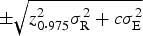
Note that the first two terms in Formula (10) are the GPQ of μ
T − μ
R and the last term is the GPQ of
 $ \pm \sqrt {z_{0 \cdot 975}^2 \sigma _{\rm R}^2 + c\sigma _{\rm E}^{\rm 2}} $
. Similar to the MLS method, the parameter of interest for Hypotheses (4) could be
 $(\mu _{\rm T} - \mu _{\rm R} )^2 - (z_{0 \cdot 975}^2 \sigma _{\rm R}^2 + c\sigma _{\rm E}^2 )$
, whose exact GPQ is
 $$\eqalign{Q & = \{ {\bar d} + Z\sqrt {h_1 ({\bf \sigma} ^2 )df_{\rm R} \displaystyle{{ms_{\rm R}} \over {U_{\rm R}}} + h_2 ({\bf \sigma} ^2 )df_{\rm E} \displaystyle{{ms_{\rm E}} \over {U_{\rm E}}}} \} ^2 \cr & \quad - z_{0{\cdot}975}^2 \displaystyle{1 \over a}df_{\rm R} \displaystyle{{ms_{\rm R}} \over {U_{\rm R}}} - \left( {c - \displaystyle{{z_{0{\cdot}975}^2} \over a}} \right)df_{\rm E} \displaystyle{{ms_{\rm E}} \over {U_{\rm E}}}}$$
Properties of
 $\bar D$
, MS
R and MS
E described earlier indicated that Z, U
R and U
E are independent random variables with exact distributions free of model parameters;
 $h_1 ({\bf \sigma} ^2 )$
and
 $h_2 ({\bf \sigma} ^2 )$
are known constants for balanced designs. Upon observing
 ${\bar d}$
, ms
R and ms
E, the distributions of GPQs listed in Formulas (10) and (11) were obtained by the following resampling algorithm.
-
Step 1. Independently sample z, u R and u E from N(0,1), χ 2(df R), and χ 2(df E).
-
Step 2. Replace Z, U R and U E in Formulas (10) and (11) with z, u R and u E. This yields q +, q − and q.
-
Step 3. Accumulate values of q +, q − and q by repeating Steps1–2 a large number of times, perhaps 5000.
This generates the resampling distributions of Q +, Q − and Q.
The inequalities of q + ⩽ 0 or q − ⩾ 0 coincide with the inequality of q ⩾ 0. As a result, the two GPQ functions for testing Hypotheses (4) yield identical GPVs given below.
 $$\eqalign{& \Pr (Q^{+} \les 0\;or\;Q^{-} \ges 0) = \Pr (Q \ges 0) \cr & \qquad \approx \displaystyle{{\hbox{number of resamples with}\ q^{+} \les 0\;or\;q^{-} \ges 0} \over {\hbox{total number of resamples}}} \cr & \qquad = \displaystyle{{\hbox{number of resamples with} q \ges 0} \over {\hbox{total number of resamples}}}}$$
Equivalence was concluded if the GPV was less than the pre-specified significance level α. Testing Hypotheses (4) could also be carried out via assessing percentiles of resampling distributions for Q
+, Q
− and Q. These percentiles are referred to as generalized CLs. Adopting the approach of two one-sided tests, H
0 was rejected when the 100αth percentile for Q
+ was greater than zero and the 100(1−α)th percentile for Q
− was less than zero. Alternatively, H
0 could be rejected when the 100(1−α)th percentile for Q was smaller than zero. The resampling algorithm for Q, however, does not produce a straightforward representation of the rejection region for
 ${\bar d}$
or
 ${\bar d}^2 $
at a given set of ms
R and ms
E values. The formulation of Q
+ and Q
− is advantageous in this regard and may be more informative to practitioners. To see this, let
 $w_{\alpha}^{+}$
be the 100αth percentile for
 $Q^{+} - {\bar d}$
. Note that
 $ - w_{\alpha}^{+}$
is the 100(1−α)th percentile for
 $Q^{-}-{\bar d}$
. Equivalence was concluded when
 $ - w_{\alpha}^{+} +{\bar d} \lt 0$
and
 $w_{\alpha}^{+}+ {\bar d} \gt 0$
. Because
 $w_{\alpha}^{+}$
depends on ms
R and ms
E only, the rejection region for
 ${\bar d}$
at given ms
R and ms
E could be effortlessly expressed as
 $ - w_{\alpha}^{+} \lt {\bar d} \lt w_{\alpha}^{+}$
. This rejection region is an empty set when
 $w_{\alpha}^{+}\lt 0$
, a situation often associated with small sample sizes and/or low
 $\sigma_{\rm R}^2 + \sigma_{\rm E}^2 $
.
Implementing the GPQ method under incomplete and unbalanced designs involved a few approximations. As stated in Property (6), U
R was approximated by a χ
2(df
R) random variable. A simple way to approximate
 $h_1 ({\bf \sigma}^2 )$
and
 $h_2 ({\bf \sigma}^2 )$
at the true value of
 ${\bf \sigma}^2 $
is to regress
 $Var(\bar D)$
on E(MS
R) and E(MS
E) in a neighbourhood of
 ${\hat{\bf \sigma}}^2$
. This was done by the algorithm presented below.
-
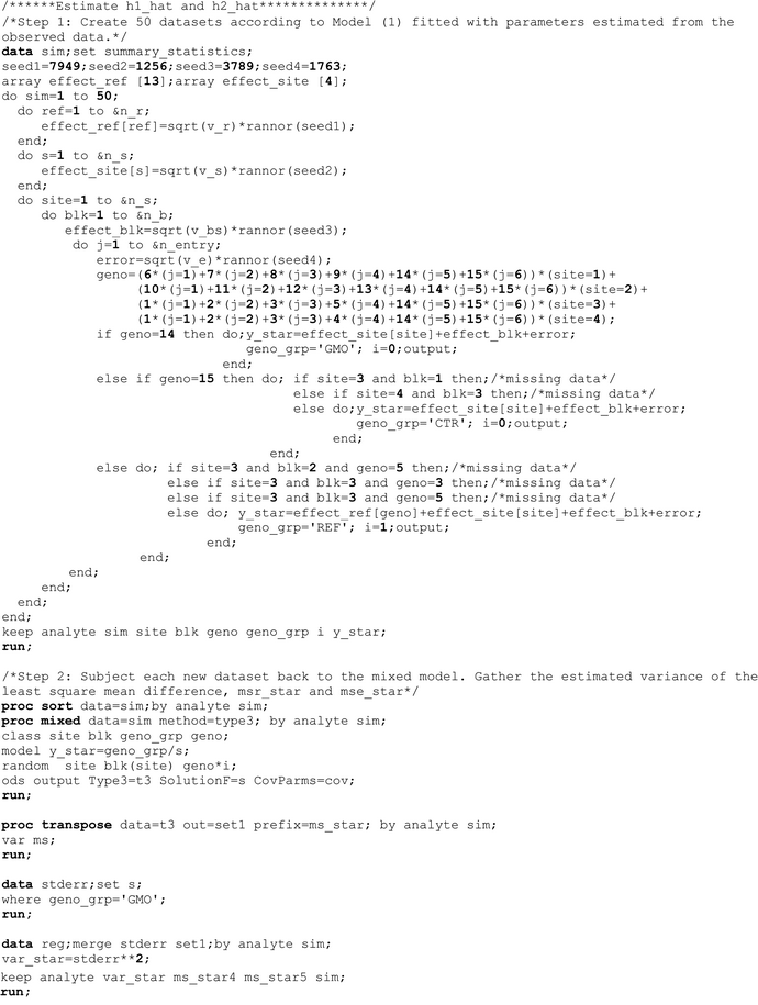
Step 1. Create a few random data sets, e.g. ten, according to Model (1) fitted with parameters estimated from the observed data. If a variance component is estimated to be negative, replace it with zero. These simulated data sets should have the same design matrix as the original data set.
-
Step 2. Apply the mixed model analysis under Model (1) to each new data set. Gather the estimated variance of the least square mean difference,
 $\hat Var(\bar D^{\ast} )$
, as well as the mean squares for reference genotype and error,
$ms_{\rm R}^{\ast} $
and
$ms_{\rm E}^{\ast} $
.
-
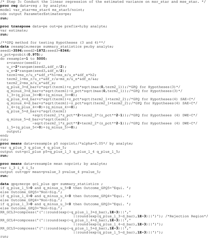
Step 3. Conduct the linear regression of
$\hat Var(\bar D^{\ast} )$
on
$ms_{\rm R}^{\ast} $
and
$ms_{\rm E}^{\ast} $
through the origin. The regression coefficients for
$ms_{\rm R}^{\ast} $
and
$ms_{\rm E}^{\ast} $
are denoted by
$\hat h_1 $
and
$\hat h_2 $
, respectively.


Now substitute
 $\hat h_1 $
and
 $\hat h_2 $
for
 $h_1 ({\bf \sigma} ^2 )$
and
 $h_2 ({\bf \sigma} ^2 )$
in Formulas (10) and (11). Afterwards statistical inference was made with respect to the resampling distributions of these novel approximate GPQs.
RESULTS
Simulation study
The proposed MLS and GPQ testing procedures were investigated by a series of simulation studies. Their type I error rates were evaluated at the boundary of the H
0 parameter space for Hypotheses (4), i.e. at
 $(\mu _{\rm T} - \mu _{\rm R} )^2 = z_{0 \cdot 975}^2 \sigma _{\rm R}^2 + c\sigma _{\rm E}^2 $
. Their power was examined inside the H
1 parameter space. Hypotheses were tested at α = 0·05 throughout. It was recognized that the relative magnitude of
 $\sigma _{\rm R}^2 $
to
 $\sigma _{\rm R}^2 + \sigma _{\rm E}^2 $
affects properties of these procedures. Define
 $\rho = \sigma _{\rm R}^2 /(\sigma _{\rm R}^2 + \sigma _{\rm E}^2 )$
. The rejection rates of the MLS and GPQ procedures were inspected at ρ = 0·1, 0·3, 0·5, 0·7 and 0·9. Ten thousand simulations were run under each parameter setting. The Monte Carlo error here was near 0·002 for type I error rate and less than 0·005 for power.
The first simulation study reviews the small-sample behaviour of the MLS and GPQ procedures for complete and balanced designs with n
R = 6, 9, 16, 20, 36 at n
S = 8 and n
B(S) = 4. The total number of field samples for each design ranges from 256 to 1216. Due to the high cost in measuring compositional endpoints, these designs may be unacceptable for producers, especially when n
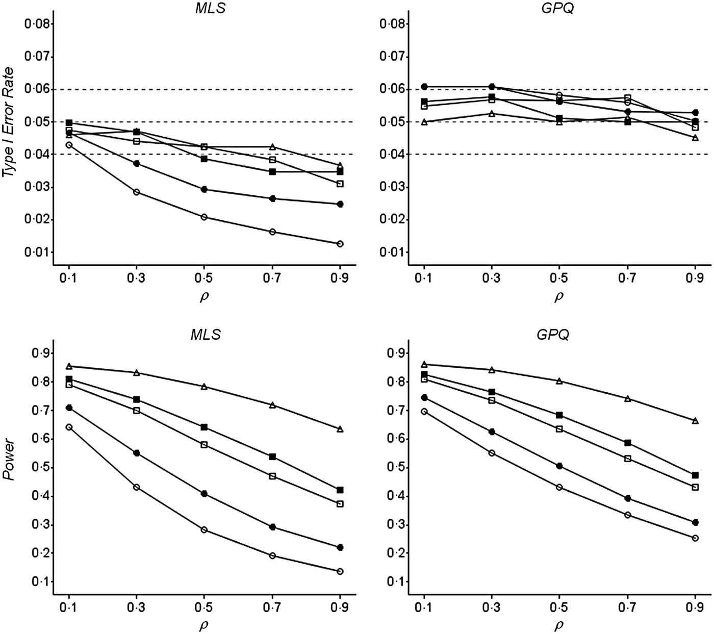
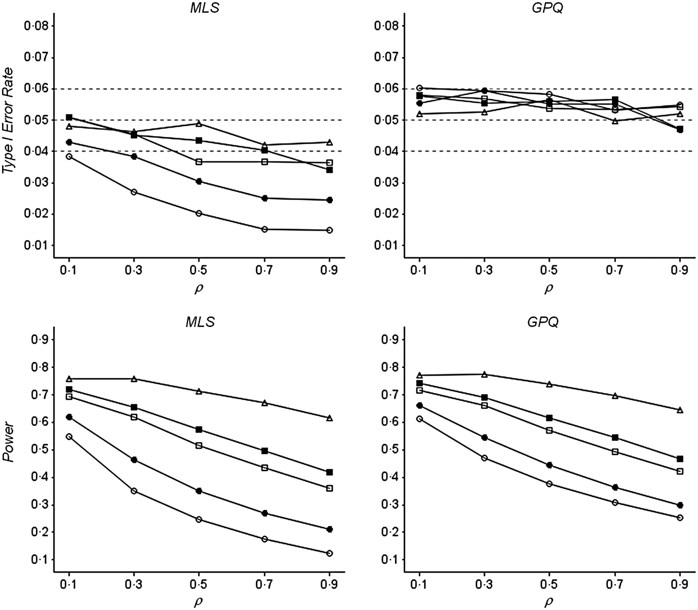
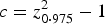
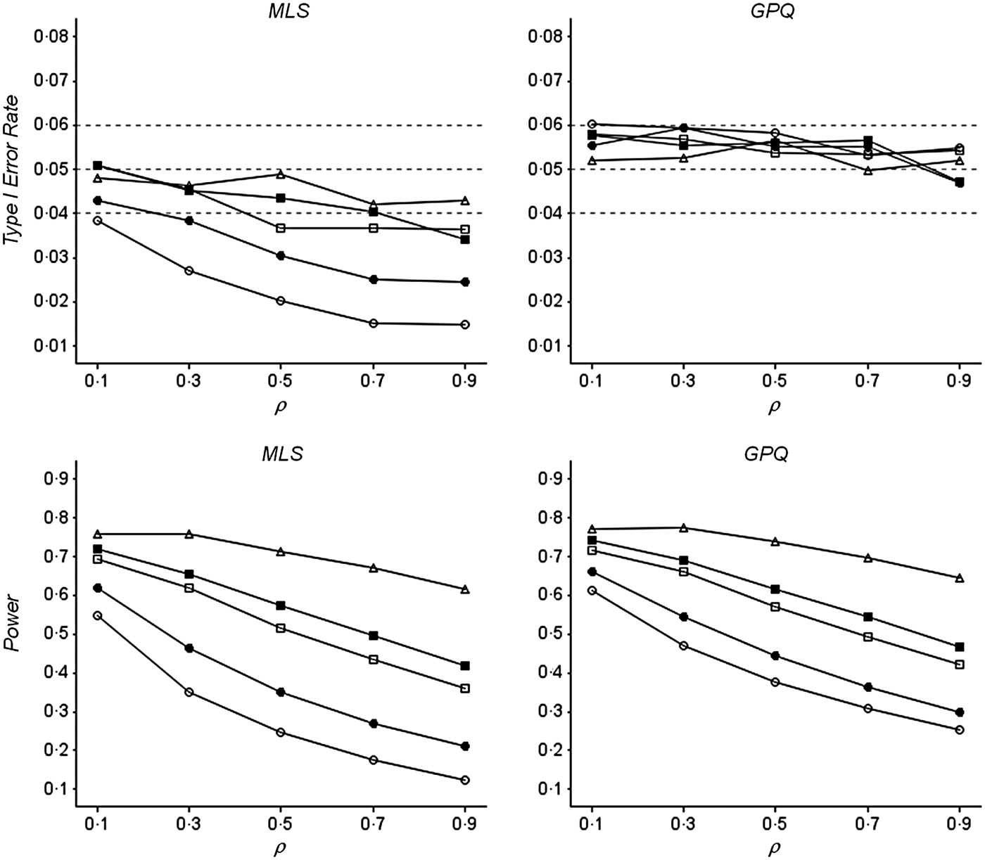
R > 6. Nonetheless, the rejection rates under these designs characterize the idealistic scenario for GMO equivalence testing. Figures 1 and 2 summarize the simulation results for testing SAE-C and DWE-C, i.e. Hypotheses (4) at
 $c = z_{0 \cdot 975}^2 $
and
 $c = z_{0 \cdot 975}^2 - 1$
. Clearly the pattern for testing SAE-C was similar to that of DWE-C. Consistent with previous experience reported in the literature, the MLS procedure concluded equivalence less often than desired. Its type I error rate deviated from the 0·05 nominal level to less than 0·02 at n
R = 6 and ρ = 0·9. This conservatism attenuated as ρ decreased or as n
R increased. The GPQ procedure, on the other hand, rejected H
0 of Hypotheses (4) with either nearly nominal or slightly liberal type I error rates. When n
R = 6 and ρ = 0·1, its type I error rate was as high as 0·06. This anti-conservatism dissipated either as n
R or ρ increased. The power of both procedures dropped as ρ ascended. It increased as n
R became larger. This is associated with the fact that inferring
 $\sigma _{\rm R}^2 $
from MS
R possesses a greater extent of uncertainty than inferring
 $\sigma _{\rm E}^2 $
from MS
E since df
E >> df
R. Consistent with their disparity in type I error rates, the GPQ procedure exceeded the MLS procedure in power.
Empirical rejection rates for testing conditional scaled average equivalence under complete balanced designs. Type I error rate was estimated at
 $(\mu _{\rm T} - \mu _{\rm R} )^2 = z_{0 \cdot 975}^2 (\sigma _{\rm R}^2 + \sigma _{\rm E}^2 )$
. Power was estimated at
 $(\mu _{\rm T} - \mu _{\rm R} )^2 = 0 \cdot 75z_{0 \cdot 975}^2 (\sigma _{\rm R}^2 + \sigma _{\rm E}^2 )$
. Dashed horizontal lines represent the 0·05 nominal level and the levels of 0·05 ± 0·01. ○, n
R = 6; ●, n
R = 9; □, n
R = 16; ■, n
R = 20; ∆, n
R = 36. GPQ, generalized pivotal quantities; MLS, modified large sample method.

Empirical rejection rates for testing conditional distribution-wise-equivalence under complete balanced designs. Type I error rate was estimated at
 $(\mu _{\rm T} - \mu _{\rm R} )^2 = z_{0 \cdot 975}^2 \sigma _{\rm R}^2 + (z_{0 \cdot 975}^2 - 1)\sigma _{\rm E}^2 $
. Power was estimated at
 $(\mu _{\rm T} - \mu _{\rm R} )^2 = 0 \cdot 75 $
 $\{ z_{0 \cdot 975}^2 \sigma _{\rm R}^2 + (z_{0 \cdot 975}^2 - 1)\sigma _{\rm E}^2 \} $
. Dashed horizontal lines represent the 0·05 nominal level and the levels of 0·05 ± 0·01. ○, n
R = 6; ●, n
R = 9; □, n
R = 16; ■, n
R = 20; ∆, n
R = 36. GPQ, generalized pivotal quantities; MLS, modified large sample method.
Next investigate equivalence testing under practical designs listed in Table 1. Rejection rates were initially simulated without the occurrence of missing data. Theoretical assumptions for the MLS and GPQ methods were satisfied under Designs I and II. For Designs III–VI, the distribution of MS
R in Formulas (9) and (10) was approximated by χ
2 (df
R); values of
 $h_1 ({\bf \sigma} ^2 )$
and
 $h_2 ({\bf \sigma} ^2 )$
were estimated via the algorithm described previously. It was observed that MS
R and MS
E regressed closely to
 $\hat Var(\bar D)$
with over 99% of adjusted coefficients of determination exceeding 0·98. This good fit supports the strategy of simplifying the dependence of
 $Var(\bar D)$
on E(MS
R) and E(MS
E) via a linear regression. Performance of the two procedures for testing SAE-C and DWE-C is presented in Figs 3 and 4, respectively. Again, similar patterns were observed when testing SAE-C and DWE-C. For each test, the MLS procedure was overly conservative unless n
R was large or ρ was close to zero. The GPQ procedure was moderately liberal. It gave high type I error rates when ρ was small. Designs III–VI in Figs 3 and 4 relate to designs in Figs 1 and 2 by having the same numbers of references, specifically n
R = 6, 9, 16, 20. At the same n
R, the GPQ procedure tended to be more liberal under unbalanced designs than balanced designs. Corresponding to their disparity in type I error rates, power of the MLS procedure was considerably lower than that of the GPQ procedure. To further mimic a real-world scenario, a random missing rate of 3% was imposed in the simulated data sets. Depending on the design, there was an average of five to eight samples missing per study. Greater rates of missing data would not be tolerated in practice and were therefore omitted. The occurrence of missing data caused
 $\sigma _{\rm S}^2 $
and
 $\sigma _{{\rm B}({\rm S})}^2 $
to appear in
 $Var(\bar D)$
, which in theory affected the behaviour of the MLS and GPQ procedures. At a 3% missing rate, the simulation results were unlikely to be sensitive to values of
 $\sigma _{\rm S}^2 $
and
 $\sigma _{{\rm B}({\rm S})}^2 $
, though. Experience with crop composition data indicates that either
 $\sigma _{\rm S}^2 $
,
 $\sigma _{\rm R}^2 $
, or, occasionally,
 $\sigma _{\rm E}^2 $
could be the dominating source of natural variation (Vahl & Kang Reference Vahl and Kang2015). Several realistic scenarios were considered here by setting
 $\sigma _{\rm S}^2 = 4$
,
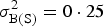 $\sigma _{{\rm B}({\rm S})}^2 = 0 \cdot 25$
,
 $\sigma _{\rm E}^2 = 1$
, and taking
 $\sigma _{\rm R}^2 \approx 0 {\cdot} {\rm 11},{\rm } 0 {\cdot} {\rm 43},{\rm 1} {\cdot} 0,{\rm 2} {\cdot} {\rm 3},{\rm 9} {\cdot} 0$
in accordance with the various levels of ρ considered. Simulation results in Figs 3 and 4 indicate that a small proportion of missing data had trivial impact on the performance of the two procedures.
Empirical rejection rates for testing conditional scaled average equivalence under various field designs (a) without missing data and (b) with 3% missing data. Type I error rate was estimated at
 $(\mu _{\rm T} - \mu _{\rm R} )^2 = z_{0 \cdot 975}^2 (\sigma _{\rm R}^2 + \sigma _{\rm E}^2 )$
. Power was estimated at
 $(\mu _{\rm T} - \mu _{\rm R} )^2 = 0 \cdot 75z_{0 \cdot 975}^2 (\sigma _{\rm R}^2 + \sigma _{\rm E}^2 )$
. Dashed horizontal lines represent the 0·05 nominal level and the levels of 0·05 ± 0·01. ○, Design I (n
R = 6); ◊, Design II (n
R = 6); ♦, Design III (n
R = 6); ●, Design IV (n
R = 9); □, Design V (n
R = 16); ■, Design VI (n
R = 20). GPQ, generalized pivotal quantities; MLS, modified large sample method.

Empirical rejection rates for testing conditional distribution-wise-equivalence under various field designs (a) without missing data and (b) with 3% missing data. Type I error rate was estimated at
 $(\mu _{\rm T} - \mu _{\rm R} )^2 = z_{0 \cdot 975}^2 \sigma _{\rm R}^2 + (z_{0 \cdot 975}^2 - 1)\sigma _{\rm E}^2 $
. Power was estimated at
 $(\mu _{\rm T} - \mu _{\rm R} )^2 = 0 \cdot 75\{ z_{0 \cdot 975}^2 \sigma _{\rm R}^2 + (z_{0 \cdot 975}^2 - 1)\sigma _{\rm E}^2 \} $
. Dashed horizontal lines represent the 0·05 nominal level and the levels of 0·05 ± 0·01. ○, Design I (n
R = 6); ◊, Design II (n
R = 6); ♦, Design III (n
R
= 6); ●, Design IV (n
R = 9); □, Design V (n
R = 16); ■, Design VI (n
R = 20). GPQ, generalized pivotal quantities; MLS, modified large sample method.

It is noteworthy that n
R, rather than the total sample size, played a crucial role in controlling the power of equivalence tests. Designs I and II collected the greatest numbers of samples but their power never ranked at the top. The total numbers of samples for Designs III and V are similar. Regarding the GPQ procedure, Design V (n
R = 16) always carried better power than Design III (n
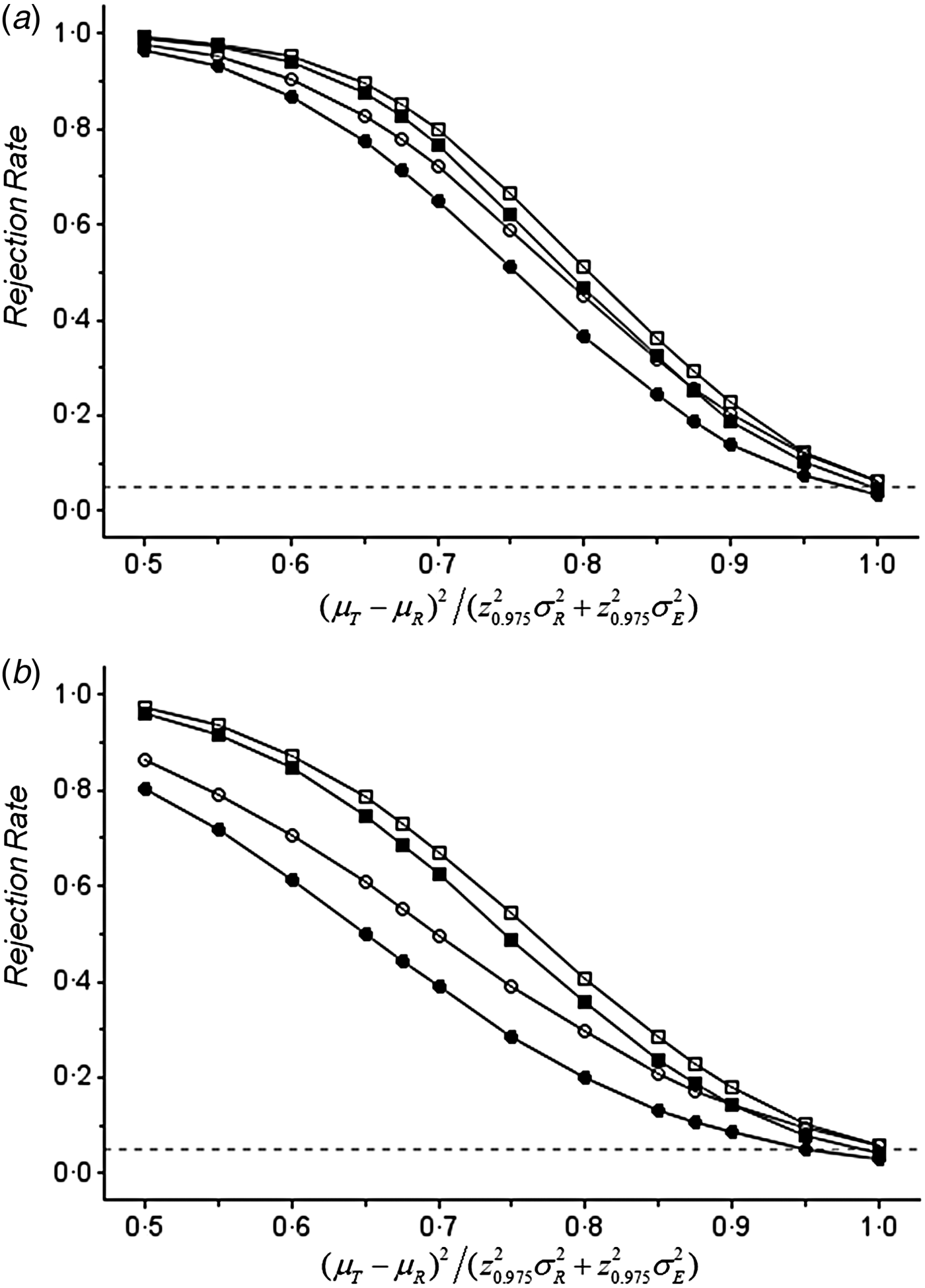
R = 6) while their type I error rates were comparable. Without missing data, Design IV has eight more samples than Design VI. Rejection rates for testing SAE-C under these two designs were plotted against
 $(\mu _{\rm T} - \mu _{\rm R} )^2 /(z_{0 \cdot 975}^2 \sigma _{\rm R}^2 + z_{0 \cdot 975}^2 \sigma _{\rm E}^2 )$
at ρ = 0·3 and 0·7 in Fig. 5. Design VI (n
R = 20) outperformed Design IV (n
R = 9) with respect to both the MLS and GPQ procedures. This superiority was more prominent at ρ = 0·7 than at ρ = 0·3. Moreover, the two power curves for Design VI differed less than those for Design IV, suggesting the reconciliation of the MLS and GPQ procedures for large n
R.
Power curves for testing conditional scaled average equivalence at (a) ρ = 0·3 and (b) ρ = 0·7. The dashed horizontal line represents the 0·05 nominal level. ○, GPQ method and Design IV; ●, MLS method and Design IV; □, GPQ method and Design VI; ■, MLS method and Design VI. GPQ, generalized pivotal quantities; MLS, modified large sample method.

Case study
Real-world data sets used in GMO safety evaluation are publicly unavailable due to proprietary reasons. As far as it is known, the illustrative example by EFSA (2010) and Van der Voet et al. (Reference Van der Voet, Perry, Amzal and Paoletti2011) is the only open document detailing the summary statistics under Model (1) for each compositional endpoint. Their analysis data set came from a study on a GM maize with n
R = 13, n
S = 4, n
B(S) = 3 and four references per site. Protocol deviation resulted in a total of 67 samples with 14, 17, 18 and 18 samples collected from the four sites. This data set, in spite of its small sample size, still holds great merit in illustrating GMO equivalence tests. Regarding the testing procedures for Hypotheses (3) and (4), summary statistics including
 $\exp ({\bar d})$
,
 $df_{\rm D} ({\hat{\bf \sigma}} ^2 )$
and
 $\sqrt {\hat Var(\bar D)} $
are directly available in Tables 4 and 5 of EFSA (2010) as well as Table 2 of Van der Voet et al. (Reference Van der Voet, Perry, Amzal and Paoletti2011). The study design and missing data pattern suggest df
R = 12, df
E = 41 and a ≈ 2·97. The observed mean squares for reference genotype and error could then be deduced according to
 $ms_{\rm R} = a\hat \sigma _{\rm R}^2 + \hat \sigma _{\rm E}^2 $
and
 $ms_{\rm E} = \hat \sigma _{\rm E}^2 $
, where
 $\hat \sigma _{\rm R}^2 $
and
 $\hat \sigma _{\rm E}^2 $
are estimated variances of reference genotype and error given by Table 2 of Van der Voet et al. (Reference Van der Voet, Perry, Amzal and Paoletti2011). It is noted that
 $\hat \sigma _{\rm R}^2 $
and
 $\hat \sigma _{\rm E}^2 $
were produced by the REML method. Although the method of moments is preferred, REML estimates are still useful for comparing testing procedures given the absence of the original data. In this example,
 $\hat \rho = \hat \sigma _{\rm R}^{\rm 2} /(\hat \sigma _{\rm R}^2 + \hat \sigma _{\rm E}^2 )$
was greater than 0·5 in 43 out of 53 analytes. For several analytes whose
 $\hat \rho $
was less than 0·3, regressing
 $\hat Var(\bar D^{\ast} )$
on
 $ms_{\rm R}^{\ast} $
and
 $ms_{\rm E}^{\ast} $
from ten simulated data sets yielded unstable estimates of
 $h_1 ({\bf \sigma} ^2 )$
and
 $h_2 ({\bf \sigma} ^2 )$
with the adjusted coefficient of determination less than 0·9. The size of the original data set, which is less than half EFSA's requirement, seems to be at fault here. Boosting the number of simulated data sets from ten to 50 appeared to tame down the instability. The Appendix provides the SAS code for testing Hypotheses (3) and (4) from summary statistics.
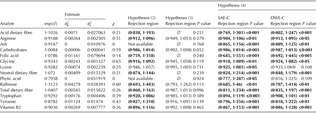
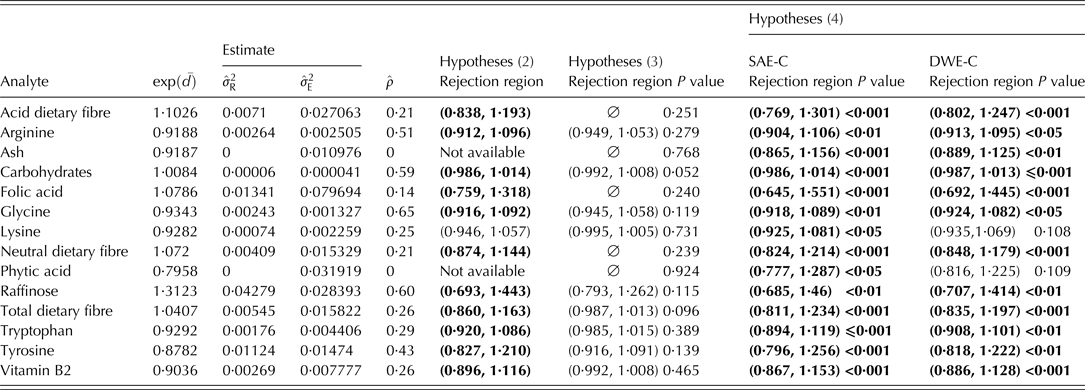
The testing procedure mandated by EFSA (2010) concluded equivalence, as defined in Hypotheses (2), for 44 of the 53 analytes. In comparison, testing Hypotheses (3) concluded equivalence for 33 analytes; testing Hypotheses (4) concluded SAE-C for 47 analytes and DWE-C for 45 analytes. Table 3 lists 14 analytes where different conclusions on equivalence occurred. Recall that the mixed model was fitted on log-transformed data. The magnitude of the difference between GMO and references is routinely assessed in terms of the ratio of their geometric means, i.e.
 $\exp ({\bar d})$
. Table 3 reports the rejection regions of
 $\exp ({\bar d})$
for these tests at given
 $\hat \sigma _{\rm R}^2 $
and
 $\hat \sigma _{\rm E}^2 $
. Note that the MLS and GPQ procedures for testing Hypotheses (4) led to identical conclusions in this example data set; but the P values and rejection regions pertaining to Hypotheses (4) are available only from the GPQ procedure.
Analytes where conclusions differ among testing procedures
DWE-C, conditional distribution-wise equivalence; SAE-C, conditional scaled average equivalence.
Values in bold indicate those cases with significant equivalence. ‘
 $\emptyset $
’ represents an empty set.
Analytes listed in Table 3 all had non-trivial
 $\hat \sigma _{\rm E}^2 $
and their values of
 $\exp ({\bar d})$
ranged from 0·80 to 1·31, which were fairly close to one. In fact, tests of SAE-C were significant for all 14 and tests of DWE-C were significant for 12 analytes. Vahl & Kang (Reference Vahl and Kang2015) pointed out the H
1 parameter space of super equivalence is nested within the H
1 parameter space of DWE-C, which in turn is nested within that of SAE-C. Coherent with this ordering, all 33 analytes significant for Hypotheses (3) were significant for SAE-C and DWE-C; all six (eight) analytes non-significant for SAE-C (DWE-C) remained non-significant for Hypotheses (3). The super equivalence defined by Hypotheses (3) was so stringent that five analytes with the lowest
 $\hat \rho $
values had the empty set as their rejection regions. Tests of Hypotheses (2) asserted equivalence more often than tests of Hypotheses (3), which is consistent with the findings of Kang & Vahl (Reference Kang and Vahl2014). Testing Hypotheses (2) and (4) disagreed on three analytes for SAE-C and two analytes for DWE-C only. This may give the false impression that the data-driven ELs are indeed acceptable. However, the apparent success of Hypotheses (2) is an artefact resulting from the insufficient number of sites. Note that the data example contains half of EFSA's minimum requirement of eight sites. Formula (12) and Fig. 3 of Kang & Vahl (Reference Kang and Vahl2014) depict the unfortunate effect that the EL of Hypotheses (2) decreases as the sample size increases. Producers adhering to EFSA's guidance will then be punished by the shrinking EL. In contrast, they will be rewarded with more significance by using well-defined ELs. Another advantage of testing Hypotheses (4) is revealed by examining the two analytes with
 $\hat \sigma _R^2 \approx 0$
, i.e. ash and phytic acid. The statistical analysis mandated by EFSA excluded them from equivalence testing and declared ‘no conclusion on equivalence’. However,
 $\hat \sigma _R^2 \approx 0$
implies
 $\sigma _R^2 $
is small relative to
 $\sigma _E^2 $
rather than being absolutely zero. The inability to test equivalence with
 $\hat \sigma _R^2 \approx 0$
is certainly an undesirable feature. The tests of SAE-C and DWE-C were both significant for ash while only the test of SAE-C was significant for phytic acid. The shortcoming of EFSA's procedure can be further highlighted by considering two extreme cases at
 $\hat \sigma _R^2 \approx 0$
. In case one, the GMO geometric mean is identical to the reference geometric mean. In case two, it is many fold larger, say a thousand. EFSA's procedure for testing equivalence would declare ‘no conclusion on equivalence’ for both cases. The proposed procedures would declare equivalence for case one and retain the null of Hypotheses (4) for case two, which satisfies common sense.
DISCUSSION
This present paper focused on the statistical procedures for evaluating the conditional equivalence of GMO to references. Both the MLS and GPQ methods were considered. In many aspects, strength of one method attends to the weakness of the other. The MLS CLs were obtained effortlessly via a simple formula. Practitioners accustomed to traditional frequentist types of inference might comprehend it more easily. The GPQ method operates under the framework of fiducial inference. Its execution requires more technical competence, since a re-sampling algorithm is needed to generate the distribution of its GPQ. Nonetheless, the convenience of the MLS method is achieved by re-expressing the original hypotheses in terms of a linear combination of expected mean squares. The resulting CLs lack meaningful interpretation. In contrast, the GPQ testing procedure is flexible with the parameterization of complex hypotheses and produces rejection regions that help practitioners visualize abstract statistical results. An additional benefit of the GPQ method comes from its ability to generate P values, which are unavailable from the MLS method. Given the fact that a P value quantifies the strength of evidence on a unit scale and substantial equivalence is established by a weight of evidence, the GPQ method is especially useful for assessing GMO across a vast number of endpoints. So far, the conservative nature of the MLS method has been viewed as a plus for regulating drugs. The simulations of McNally et al. (Reference McNally, Iyer and Mathew2003) and Chiu et al. (Reference Chiu, Tsai and Liu2010) show that the MLS method did not suffer a severe power loss over the range of parameter values commonly encountered in bioequivalence studies. The disparity between the MLS and GPQ methods in their statistical properties was more distinctive for testing GMO equivalence. Simulation, tailored toward the unique setting of GMO safety evaluation, showed that the MLS method could be extremely conservative while the GPQ method was mildly liberal. The majority of compositional endpoints had small
 $\sigma _{\rm E}^2 $
relative to
 $\sigma _{\rm R}^2 $
. In these cases, the GPQ method is preferred because of its near-nominal type I error rate and superior power. For those few endpoints where
 $\sigma _{\rm R}^2 $
was observed to be much smaller than
 $\sigma _{\rm E}^2 $
, the MLS method had a tight control over the type I error rate and is therefore recommended in such cases. Simulation results also indicate that the two methods had good power under practical designs; power of the GPQ method always exceeded that of the MLS method; their difference may not be practically noticeable for large samples or when
 $\sigma _{\rm R}^2 $
is relatively large compared with
 $\sigma _{\rm E}^2 $
. The case study of real-world data further demonstrated the utility of the two proposed procedures as compared with the procedure currently mandated by EFSA.
The theory supporting the MLS and GPQ methods requires independent summary statistics with identifiable distributions which are attainable only in idealistic situations. Real-world studies bear incomplete and unbalanced arrangements (as in multi-site field designs), intricate correlations (as in clinical crossover designs), and/or incidental missing data. These practical issues make it difficult to construct summary statistics that satisfy the exact requirements. Simulation studies under one-way random effect models demonstrate that the MLS and GPQ methods were quite lenient towards moderate violations of theoretical assumptions with respect to parameter estimation (Park & Burdick Reference Park and Burdick2003; Krishnamoorthy & Mathew Reference Krishnamoorthy and Mathew2004; Krishnamoorthy & Lian Reference Krishnamoorthy and Lian2012). Bioequivalence has been successfully tested via MLS and GPQ methods that ignored some of the theoretical requirements (Hyslop et al. Reference Hyslop, Hsuan and Holder2000; McNally et al. Reference McNally, Iyer and Mathew2003). The mild impact of an unbalanced design matrix was also seen in the empirical type I error rates of these two methods under Model (1). Nonetheless, producers are encouraged to pursue the balanced design described by John & Mitchell (Reference John and Mitchell1977) and to include adequate replicates of random effects so as to enhance power. Missing data should be minimized as it is often indicative of poor study conduct. Performance of equivalence tests should also be routinely monitored through simulation.
In the past decade, there have been intense debates over the proper steps to ascertain GMO substantial equivalence to conventional food crops (Hothorn & Oberdoerfer Reference Hothorn and Oberdoerfer2006; Herman et al.
Reference Herman, Scherer, Phillips, Storer and Krieger2010; Van der Voet et al.
Reference Van der Voet, Perry, Amzal and Paoletti2011; Kang & Vahl Reference Kang and Vahl2014; Vahl & Kang Reference Vahl and Kang2015). A viable solution is best obtained via integrating biological reasoning with statistical justification. Conditional equivalence compares GMO and references based on their conditional distributions. In contrast, super equivalence judges the mean of GMO against the super-distribution of reference genotype means. Super-equivalence may first appear to be the natural choice for assessing GMO. However, its biological relevance is lost when
 $\sigma _{\rm R}^2 $
does not dominate crop natural variation. Conditional equivalence circumvents this issue by also incorporating the variability due to plot, analytical error, etc. This approach resonates with the concept of site-specific equivalence advocated by EFSA (2010). Equivalence testing facilitates hazard identification with statistical rigour. It adheres to the strategy of König et al. (Reference König, Cockburn, Crevel, Debruyne, Grafstroem, Hammerling, Kimber, Knudsen, Kuiper, Peijnenburg, Penninks, Poulsen, Schauzu and Wal2004) and serves as the first step in GMO risk assessment. The resulting non-significant endpoints become candidates for hazard characterization, which involves a thorough exposure assessment and possible lab animal testing. A recent explanatory statement of EFSA (2014) elaborates that the assessment of GMO compositional and agronomic-phenotypic characteristics serves as the basis for determining the design, conduct and interpretation of their mandated 90-day rodent study. In the real-world data example, 20 endpoints failed the test for super-equivalence, among which 12 or 14 were significant in testing conditional equivalence. Note that this discrepancy occurred mostly at endpoints with non-trivial
 $\sigma _{\rm E}^2 $
and the corresponding GMO-reference ratios of geometric means were all fairly close to one. Testing for conditional equivalence appears to avoid excessive investigation on endpoints where the deviation of GMO from references is unlikely to be of biological importance. For these reasons, conditional equivalence is more suitable for GMO safety evaluation than super-equivalence. The two forms of conditional equivalence both have statistical and biological merits: SAE-C may be favoured by some because of its lenient requirement and simple, non-technical interpretation whereas DWE-C may be preferred by others because its ELs assign a lighter weight to the error term variance shared by the GMO and reference distributions. The ultimate call should be made through an open dialogue among stakeholders with clear interests (the ag-biotech industry and regulatory authorities) as well as researchers with independent, scientific opinions.
A controversial topic in GMO safety evaluation revolves around the usage of Model (1). Genotype × site interaction, also known as G × E with E standing for environment, is an indispensable source of variation in analysing field efficacy of experimental crops. Ward et al. (Reference Ward, Nemeth, Brownie, Hong, Herman and Oberdoerfer2012) criticized Model (1) for its omission of G × E terms. In the latest public comments to EFSA's draft guidance on GMO, one organization described G × E as a known important effect on crop composition (EFSA 2015a ). This comment cited the article by Whent et al. (Reference Whent, Hao, Slavin, Zhou, Song, Kenworthy and Yu2009) who reported G × E constituted over half of the variation in some compositional endpoints. The EFSA (2015b ) responded by mandating an analysis of G × E via a separate fixed effect model in the case of ‘significant differences [from the control] and/or lack of equivalence [to the references]’. A closer look at the analysis conducted by Whent et al. (Reference Whent, Hao, Slavin, Zhou, Song, Kenworthy and Yu2009) reveals that percentages of the total mean square for genotype, site and G × E were used to measure their respective contribution to variation under a fixed effect model. Recall that expectation of each mean square equals the error term variance plus a quadratic form quantifying fixed effects. Small percentages of genotype and site in Whent et al. (Reference Whent, Hao, Slavin, Zhou, Song, Kenworthy and Yu2009) always coincided with large error term variances. The observed large contribution from G × E, although significantly non-zero, became less relevant after taking the experimental design and the error term variance into account. Therefore, these results point to the importance of the error term, rather than G × E. A proper way to study sources of variation is to conduct a variance component analysis under the random and/or mixed effect model. It is interesting to note that in several variance component analyses on GM crops, the effect of G × E was negligible in comparison with the magnitude of variation due to site, reference genotype and the error term (Harrigan et al. Reference Harrigan, Culler, Culler, Breeze, Berman, Halls and Harrison2013; Harrison et al. Reference Harrison, Howard, Malven, Halls, Culler, Harrigan and Wolfinger2013; Venkatesh et al. Reference Venkatesh, Breeze, Liu, Harrigan and Culler2014). These findings provide empirical justification that Model (1) is indeed adequate for assessing GMO safety with respect to compositional endpoints. The influence of G × E on agronomic-phenotypic endpoints can only be clarified through proper statistical analyses on an abundance of real-world data. The proposed MLS and GPQ methods, in addition to their usage in equivalence testing, serve as valuable tools for characterizing crop natural variation. A compelling GMO safety evaluation requires solid biological exploration accompanied by sound statistical justification. It is hoped that the present work further advances the progress of a science-based decision-making process.
APPENDIX: SAS code for the case study