1. Introduction
Acoustic pressure reconstruction from near-field flows is a fundamental problem in identification of the sound sources. The ESM is one of the popular methods for acoustic pressure reconstruction (Bi et al. Reference Bi, Chen, Chen and Zhou2005; Lee Reference Lee2017; Fernandez-Grande, Xenaki & Gerstoft Reference Fernandez-Grande, Xenaki and Gerstoft2017). The ESM replaces a radiator or scattering body by multipoles, called equivalent sources. The strengths of equivalent sources are determined by matching the acoustic pressure or acoustic pressure gradient at points, called collocation points, outside or on the solid boundary. The ESM has advantages compared with traditional methods in efficiency and flexibility (Lee Reference Lee2017). However, it suffers from numerical instability as well as disturbances of near-field flow. The numerical instability results from the ill-conditioned systems of linear equations for solving equivalent sources’ strengths. Different methods have been proposed to address the numerical instability problem of ESM (Fahnline & Koopmann Reference Fahnline and Koopmann1991; Lee et al. Reference Lee, Brentner and Morris2010, Reference Lee, Brentner and Morris2011; Xu, Mao & Hu Reference Xu, Mao and Hu2019; Wang et al. 2022). A detailed summary of some techniques for numerical instability can be found in Lee (Reference Lee2017). While the numerical stability has been greatly improved in the last decades, the disturbances of the near-field flow have not been delimited until recently.
A direct approach to suppress disturbances of near-field flows is to place collocation points in the linear acoustic region with negligible hydrodynamic pressure. Since the hydrodynamic pressure decays faster than the acoustic pressure from the near field to far field, the collocation points are usually placed sufficiently far from the acoustic sources at the cost of the resolution of the reconstructed acoustic pressure field (Papamoschou Reference Papamoschou2011, Reference Papamoschou2018). Papamoschou (Reference Papamoschou2011) successfully modelled the jet noise spectra from the pressure in the linear acoustic region through including the monopole source to represent the localized sources.
Another approach to suppress the disturbances of hydrodynamic pressure is to separate the hydrodynamic pressure from the near-field pressure. Early efforts relied on spectral filtering, making assumptions about frequency segregation. Arndt, Long & Glauser (Reference Arndt, Long and Glauser1997) and Coiffet et al. (Reference Coiffet, Jordan, Delville, Gervais and Ricaud2006) noted that the hydrodynamic component dominates the low-frequency region of the spectrum, while the acoustic component is more prominent at high frequencies. They achieved the separation between the acoustic and hydrodynamic components with a low-pass or high-pass filter. This evolved into wavenumber–frequency Fourier filtering, leveraging differences in phase velocity (Kerhervé et al. Reference Kerhervé, Guitton, Jordan, Delville, Fortuné, Gervais and Tinney2008; Tinney & Jordan Reference Tinney and Jordan2008). A major step forward was the introduction of wavelet-transform techniques (Grizzi & Camussi Reference Grizzi and Camussi2012; Mancinelli et al. Reference Mancinelli, Pagliaroli, Di Marco, Camussi and Castelain2017; Li, Rival & Wu Reference Li, Rival and Wu2021). This method moved beyond earlier global spectral assumptions by targeting the time-localized, intermittent nature of hydrodynamic events, which led to a more robust separation. Concurrently, physics-based decomposition techniques have emerged as a distinct approach for analysing high-speed flow fields. Rooted in the foundational framework of Kovasznay (Reference Kovasznay1953), these methods decompose fluctuations into vortical, acoustic and entropic modes. A natural approach utilizes the Helmholtz decomposition to separate the flow field into solenoidal (rotational, incompressible) and dilatational (irrotational, compressible) components, which have been widely applied to study compressibility effects in turbulent flows (Pirozzoli, Bernardini & Grasso Reference Pirozzoli, Bernardini and Grasso2010; Jagannathan & Donzis Reference Jagannathan and Donzis2016; Wang, Gotoh & Watanabe Reference Wang, Gotoh and Watanabe2017). A key advance beyond the Helmholtz decomposition is momentum potential theory (Doak Reference Doak1995, Reference Doak1998). The momentum potential theory shifts the focus to the momentum density field, providing a unified framework that separates hydrodynamic, acoustic and entropic components, enabling the identification of noise sources and energy pathways within the flow (Unnikrishnan & Gaitonde Reference Unnikrishnan and Gaitonde2016). Given the fundamental importance of separation of hydrodynamic and acoustic components, there still exists a substantial body of additional work.
Recently, Zhou et al. (Reference Zhou, Zang, Liu and Wang2025) proposed the filtered pressure-based ESM (FESM), an acoustic extrapolation technique that leverages the propagation characteristics of pressure to reconstruct the far-field from near-field flow data. The FESM obtains filtered pressure by implementing a convection operator on pressure, inspired by the work of Zhong & Zhang (Reference Zhong and Zhang2017, Reference Zhong and Zhang2018a , Reference Zhong and Zhangb ). Strengths of the equivalent sources are then computed from the filtered pressure, and the far-field acoustic pressure is reconstructed from these sound sources. Through the FESM, the sensitivity of sound prediction to collocation points’ locations is notably suppressed. However, the FESM is based on Taylor’s frozen flow hypothesis. The hydrodynamic components are assumed to be convected by mean flow or uniform free stream. Therefore, FESM is only applicable to cases where the collocation points are located in regions with weak vortex interactions. In fact, the convection velocity of pressure has been reported to be scale-dependent (Bull Reference Bull1967; Abraham & Keith Reference Abraham and Keith1998; Yang & Yang Reference Yang and Yang2022). Moreover, during the convection motion, the intensity of the hydrodynamic component also changes continuously (Lowson Reference Lowson1965; Noack & Eckelmann Reference Noack and Eckelmann1994; Sarwar et al. Reference Sarwar, Mansy, Reda, Josep and Mellibovsky2023; Aleksyuk & Heil Reference Aleksyuk and Heil2024), thus not accurately satisfying the frozen flow hypothesis. This leads to the failure of the FESM to completely filter hydrodynamic pressure in vortical flows with strong interactions.
This work proposes a hierarchically FESM (HESM) to reconstruct the far-field acoustic pressure from vortical flows with strong interactions. The HESM replaces the convection velocity in Taylor’s frozen flow hypothesis as an adaptive complex variable to better capture the multiscale nature of hydrodynamic pressure. The spurious source associated multiscale convection and the spatial amplification of the hydrodynamic pressure can thus be suppressed. The acoustic component can be obtained by implementing a convection operator with the complex convection velocity on the near-field pressure. By iteratively updating the complex convection velocity and the filtered pressure, the proposed approach enables the simultaneous acquisition of the reconstructed acoustic pressure field and the governing equations for hydrodynamic pressure.
The remainder of this paper is organized as follows. The details of the proposed HESM are given in § 2. Validations of the proposed approach with two-dimensional (2-D) convecting vortex and laminar and turbulent flows over a circular cylinder are presented in § 3. Finally, the conclusions are drawn in § 4.
2. Hierarchical reconstruction of acoustic pressure
The basic idea of the ESM is to place virtual sources with undetermined strengths in space and to collect acoustic variables on collocation points, as shown in figure 1. The acoustic variable
 $\phi$
on the collocation point
 ${\boldsymbol {y}}_{\boldsymbol {c}}$
can be expressed as
 \begin{align} \begin{split} \phi \left ( {{{\boldsymbol {y}}_{\boldsymbol {\kern-1pt c}}};\omega } \right ) = \sum \limits _j {{S}({{\boldsymbol {y}}_{\kern-1pt j}},\omega )} G({{\boldsymbol {y}}_{\boldsymbol {\kern-1pt c}}},{{\boldsymbol {y}}_{\kern-1pt j}};\omega ), \end{split} \end{align}
where
 $\omega$
is the source frequency,
 $\boldsymbol{y}$
is the source position,
 ${S}({{\boldsymbol {y}}_{\kern-1pt j}},\omega )$
is the strength of the jth equivalent sound source. According to the work of Dunn & Tinetti (Reference Dunn and Tinetti2004), the equivalent sources can be taken as monopole sources. Here
 $G$
is Green’s function of the convected wave equation. The formulation of
 $G$
is selected depending on the dimensionality of the flow. The acoustic variable
 $\phi$
can be acoustic pressure fluctuation (Dunn & Tinetti Reference Dunn and Tinetti2004; Wang et al. 2022), acoustic velocity (Mao et al. Reference Mao, Zhang, Xu and Qi2015; Siozos-Rousoulis et al. Reference Siozos-Rousoulis, Amoiridis, De, Tim, Anestis and Ghorbaniasl2019) and acoustic pressure gradient (Lee, Brentner & Morris Reference Lee, Brentner and Morris2011; Wang et al. Reference Wang, Rienstra, Bi and Koren2020). We will refer to the ESM directly using pressure fluctuations as PESM. Using these acoustic variable
 $\phi$
as input, the strengths
 ${S}({{\boldsymbol {y}}_{\kern-1pt j}},\omega )$
of the equivalent sources can be determined by solving the equation as follows:
 \begin{align} \boldsymbol{b} = \boldsymbol{Aq}. \end{align}
Here,
 $\boldsymbol{A}$
is an
 $N_c \times N_s$
matrix whose
 $(n_c,n_s)$
th element is given by Green’s function
 $G(\boldsymbol{y}_{\mathrm{c},n_c},\boldsymbol{y}_{n_s};\omega )$
, where
 $n_s = 1,2,\ldots ,N_s$
(row index) corresponds to the
 $m$
th equivalent source, and
 $n = 1,2,\ldots ,N$
(column index) corresponds to the
 $n$
th collocation point. The column vector
 $\boldsymbol{q} = [q_1, q_2, \ldots , q_{N_s}]^\top$
contains the
 $N_s$
unknown strengths of the equivalent sources. The vector
 $\boldsymbol{b}$
on the left-hand side is a known
 $N_c$
-dimensional vector; its
 $n_c$
th element is the measured sound pressure
 $\phi (\boldsymbol{y}_{\mathrm{c},n_c};\omega )$
at the
 $n_c$
th collocation point. With the equivalent sound sources, the sound variable at field point
 $\boldsymbol {x}$
can be reconstructed as follows:
 \begin{align} \begin{split} \phi \left ( {{\boldsymbol {x}};\omega } \right ) = \sum \limits _j {{S}({{\boldsymbol {y}}_{\kern-1pt j}},\omega )} G({\boldsymbol {x}},{{\boldsymbol {y}}_{\kern-1pt j}};\omega ). \end{split} \end{align}
Schematics of the ESM for prediction of sound generated from flows over a circular cylinder.

Due to the hydrodynamic pressure in the flow, direct use of near-field flow in determining the equivalent sources tends to result in significant overprediction of aerodynamic sound (Nitzkorski & Mahesh Reference Nitzkorski and Mahesh2014; Ikeda et al. Reference Ikeda, Enomoto, Yamamoto and Amemiya2017; Zhou et al. Reference Zhou, Zang, Liu and Wang2025). Recently, to filter out the hydrodynamic component from the near-field flow variable, Zhong & Zhang (Reference Zhong and Zhang2018a
,Reference Zhong and Zhang
b
) proposed performing the convection operator
 ${D_c} = {\textrm {i}}\omega + {{\boldsymbol {u}}_{\boldsymbol {c}}}\boldsymbol{\cdot }\boldsymbol{\nabla}$
on the pressure with respect to
 $\boldsymbol {x}$
and obtain a sound extrapolation method based on the filtered pressure
 $D_c(p')$
, where
 ${\boldsymbol {u}}_{\boldsymbol {c}}$
is the convection velocity of the hydrodynamic pressure. The convection velocity was usually chosen to be the uniform free stream velocity and mean flow velocity, which are both frequency-invariant (Zhong & Zhang Reference Zhong and Zhang2018b
; Zhou et al. Reference Zhou, Zang, Liu and Wang2025). However, in turbulence, the convection velocity of hydrodynamic pressure is dependent on scale and frequency (Bull Reference Bull1967; Yang & Yang Reference Yang and Yang2022). This is due to fact that large-scale structures are convected at a nearly uniform speed that is proportional to the bulk velocity, whereas small-scale structures travel at the local mean velocity (Del Alamo & Jiménez Reference Del Alamo and Jiménez2009). Additionally, hydrodynamic pressures experience amplitude variation during convection due to the instability of the shear layer and viscous dissipation (Lowson Reference Lowson1965; Noack & Eckelmann Reference Noack and Eckelmann1994; Sarwar et al. Reference Sarwar, Mansy, Reda, Josep and Mellibovsky2023; Aleksyuk & Heil Reference Aleksyuk and Heil2024). To address the limitation of Taylor’s frozen flow hypothesis with frequency-invariant convection velocity, we propose a hierarchical method to reconstruct the acoustic pressure from near-field flows.
According to the work of Kovasznay (Reference Kovasznay1953), different flow variable fluctuations can be decomposed into acoustic, vortical and entropy modes. Despite the decomposition being under the assumption of a small-amplitude disturbance, use of this decomposition leads to more accurate prediction of acoustic pressure (Zhong, Chen & Zhou Reference Zhong, Chen and Zhou2024). In this work, we focus on subsonic flows and the entropy modes are neglected. Thus, the pressure fluctuation is expressed as the sum of the acoustic pressure fluctuation
 $p'_a$
and the hydrodynamic pressure fluctuation
 $p'_v$
, i.e.
 \begin{align} \begin{split} p' = p'_a + p'_v. \end{split} \end{align}
We propose a frequency-domain convection operator
 ${D_v} = {\textrm {i}}\omega + {{\boldsymbol {u}}_{\boldsymbol {v}}}\boldsymbol{\cdot }\boldsymbol{\nabla}$
to filter out the hydrodynamic pressure. It is postulated that the hydrodynamic pressure fluctuation
 $p'_v$
satisfies the convective relation
 \begin{align} \begin{split} {\textrm {i}}\omega {p'_v} + {{\boldsymbol {u}}_{\boldsymbol {v}}}\boldsymbol{\cdot }\boldsymbol{\nabla }{p'_v}=0. \end{split} \end{align}
Here,
 $ \boldsymbol{u}_v$
is defined as a complex variable that varies with spatial position
 $ \boldsymbol{y}$
and frequency
 $ \boldsymbol{\omega }$
to capture both the phase and amplitude variations of the hydrodynamic pressure. Although the convection velocity typically describes only phase variation, we still refer to the complex variable
 $ \boldsymbol{u}_v$
as the complex convection velocity to distinguish it from the free stream and mean velocities used in previous studies (Zhong & Zhang Reference Zhong and Zhang2018a
; Zhou et al. Reference Zhou, Zang, Liu and Wang2025). The direction of the complex convection velocity
 $ {{\boldsymbol {u}}_{\boldsymbol {v}}}$
is defined as
 $\boldsymbol{\hat u}$
. The complex convection velocity can thus be expressed as
 ${{\boldsymbol {u}}_{\boldsymbol {v}}} = {u_{{v1}}}({\boldsymbol {y}},\omega ){e^{{{i}}{\theta _{v1} }({\boldsymbol {y}},\omega )}}{\boldsymbol{\hat u}}$
, where
 $u_{{v1}}$
and
 $\theta _{v1}$
represent the magnitude and phase of the complex convection velocity. The convective direction of hydrodynamic pressure is typically associated with the location of the collocation points relative to the solid body. At positions sufficiently far from the body, where vertical and lateral velocities are negligible compared with the streamwise component, the convective direction may align with the uniform free stream. However, for collocation points in close proximity to the body or within recirculation zones, the convection of hydrodynamic pressure perpendicular to the free stream needs to be taken into account. In this study, the collocation points are positioned at a substantial distance from the solid boundary.
Inspired by the structure of deep multilayer perceptrons, the unknown part of complex convection velocity
 $ {{\boldsymbol {u}}_{\boldsymbol {v}}}$
is expressed as a function of near-field pressure in the following hierarchical form:
 \begin{align} \begin{split} {{u_{{v1}}}({\boldsymbol {y}},\omega ){e^{{{i}}{\theta _{v1} }({\boldsymbol {y}},\omega )}}} = F^{(L)} \big ( F^{(L-1)} \big ( {\cdots} F^{(1)}(p') {\cdots} \big ) \big ). \end{split} \end{align}
Compared with the uniform free stream or mean flow convection velocity used in the frozen-flow assumption, the complex convection velocity is defined as varying with spatial position and frequency. Therefore, the complex convection velocity is able to represent convection at different time scales. Additionally, the complex convection velocity includes an extra phase component compared with the traditional convection velocity, allowing it to represent the spatial variation of the hydrodynamic pressure’s amplitude. More detailed discussion of the complex convection velocity can be found in Appendix A. For the convenience of writing, we denote
 ${u_{v1}}({\boldsymbol {y}},\omega ){e^{{{i}}{\theta _{v1}}({\boldsymbol {y}},\omega )}}$
as
 $u_v$
hereinafter. The mapping function
 $F$
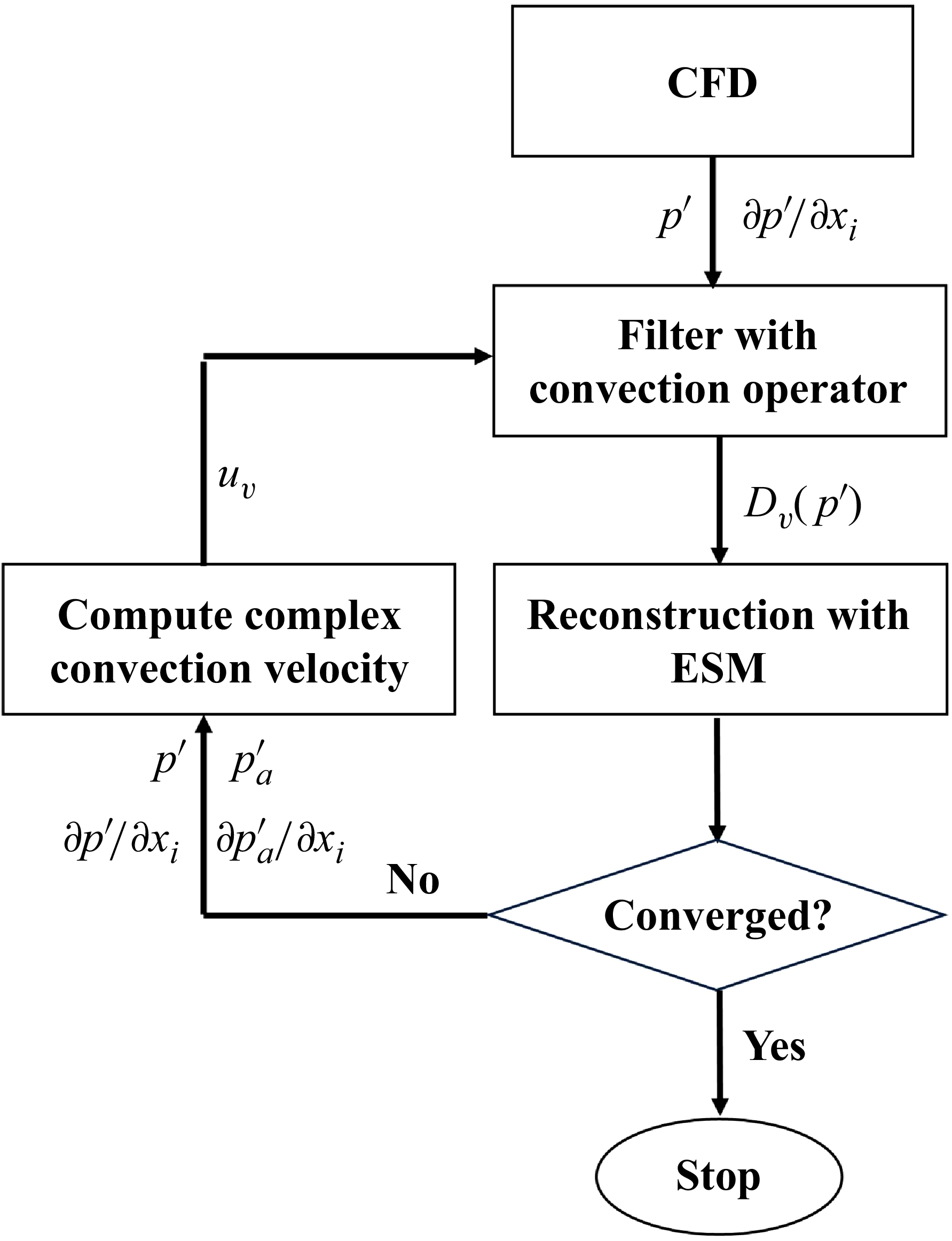
of each layer can be determined through the following process. As shown in figure 2, in the initial iteration step, we set
 $ u_v$
to the free stream speed
 $U$
. The initial strength of equivalent sources can be solved using
 \begin{align} \begin{split} {D_v }\left [ {p'\left ( {{{\boldsymbol {y}}_{\boldsymbol {\kern-1pt c}}};\omega } \right )} \right ]=&{D_v }\left [ {\sum \limits _j {{S}({{\boldsymbol {y}}_{\kern-1pt j}},\omega )} G({{\boldsymbol {y}}_{\boldsymbol {\kern-1pt c}}},{{\boldsymbol {y}}_{\kern-1pt j}};\omega )} \right ]\\ =&{\sum \limits _j {{S}({{\boldsymbol {y}}_{\kern-1pt j}},\omega )} {D_v }\left [G({{\boldsymbol {y}}_{\boldsymbol {\kern-1pt c}}},{{\boldsymbol {y}}_{\kern-1pt j}};\omega ) \right ]}. \end{split} \end{align}
Then, the acoustic pressure fluctuation
 $ p'_a$
and its derivative along the
 $x_i$
axis
 $\partial p{'_a}/\partial {x_i}$
can be obtained as follows:
 \begin{align} \begin{split} {p'_a}\left ( {{\mathbf{x}};\omega } \right ) &= \sum \limits _j {S({{\boldsymbol {y}}_{\kern-1pt j}},\omega )} G({\mathbf{x}},{{\boldsymbol {y}}_{\kern-1pt j}};\omega ),\\ \frac {{\partial {p'_a}\left ( {{\mathbf{x}};\omega } \right )}}{{\partial {x_i}}} &= \sum \limits _j {S({{\boldsymbol {y}}_{\kern-1pt j}},\omega )} \frac {{\partial G({\mathbf{x}},{{\boldsymbol {y}}_{\kern-1pt j}};\omega )}}{{\partial {x_i}}}. \end{split} \end{align}
The new hydrodynamic pressure fluctuation
 $ p'_v$
and and its spatial derivative
 $\partial p{'_v}/\partial {x_i}$
can then be derived from
 \begin{align} \begin{split} p'_v &= p' - p'_a, \\ \partial p{'_v}/\partial {x_i} &= \partial p'/\partial {x_i} - \partial p{'_a}/\partial {x_i}. \end{split} \end{align}
By introducing the definition of the complex convection velocity, the governing equation for the hydrodynamic pressure (2.5) can be formulated as
 \begin{align} \begin{split} {\textrm {i}}\omega {p'_v} + {u_v}\left ( {{{\hat u}_i}\frac {{\partial {{p'}_v}}}{{\partial {x_i}}}} \right ) = 0. \end{split} \end{align}
By using the new
 $ p'_v$
and
 $\partial p{'_v}/\partial {x_i}$
, we can update the complex convection velocity
 $ {{\boldsymbol {u}}_{\boldsymbol {v}}}$
from (2.10) as
 \begin{align} \begin{split} {u_v} = \frac {{ - {\textrm {i}}\omega p{'_v}}}{{\frac {{\partial p{'_v}}}{{\partial {x_i}}}{{\hat u}_i}}}. \end{split} \end{align}
The updated complex convection velocity
 $u_v$
is expected to be more accurate, as it is now computed using the refined hydrodynamic pressure fluctuation
 $p_v'$
. Substituting the updated complex convection velocity
 $ {\boldsymbol {u}}_{\boldsymbol {v}}$
into the convection operator to filter out hydrodynamic pressure, we obtain
 \begin{align} \begin{split} {D_v}(p{'})=({\textrm {i}}\omega + {{\boldsymbol {u}}_{\boldsymbol {v}}}\boldsymbol{\cdot }\boldsymbol{\nabla })p'. \end{split} \end{align}
The hydrodynamic pressure is thus further filtered out with updated
 ${\boldsymbol {u}}_{\boldsymbol {v}}$
. By continuously iterating through (2.7) to (2.12), we can obtain a new governing equation for the hydrodynamic pressure fluctuation
 $ p'_v$
and improve the prediction if the acoustic pressure fluctuation
 $ p'_a$
. As shown in figure 2, using numerical simulation as an example, the detailed implementation steps are as follows. First, sample the pressure fluctuation
 $ p'$
and its derivative
 $ \partial p' / \partial x_i$
from numerical simulation, and initialize
 $ \boldsymbol{u_v}$
and
 $ D_v(p')$
. Next, compute the acoustic pressure fluctuation
 $ p'_a$
using (2.7) and (2.8). Then, compute the hydrodynamic pressure fluctuation
 $ p'_v$
using (2.9). After that, update
 $ \boldsymbol{u_v}$
using (2.11). Finally, filter out the pressure fluctuation using (2.12) and return to the second step of computing the acoustic pressure to repeat the process.
Flowchart illustrating the hierarchical reconstruction of acoustic and hydrodynamic pressure.

We note that the FESM proposed by Zhou et al. (Reference Zhou, Zang, Liu and Wang2025) is a reduced form of the method proposed in this work. The HESM with only one iteration reduced to the FESM proposed by Zhou et al. (Reference Zhou, Zang, Liu and Wang2025), where the strengths of the equivalent sources are determined using
 \begin{align} \begin{split} {D_c }\left [ {p'\left ( {{{\boldsymbol {y}}_{\boldsymbol {\kern-1pt c}}};\omega } \right )} \right ]=&{D_c }\left [ {\sum \limits _j {{S}({{\boldsymbol {y}}_{\kern-1pt j}},\omega )} G({{\boldsymbol {y}}_{\boldsymbol {\kern-1pt c}}},{{\boldsymbol {y}}_{\kern-1pt j}};\omega )} \right ]\\ =&{\sum \limits _j {{S}({{\boldsymbol {y}}_{\kern-1pt j}},\omega )} {D_c }\left [G({{\boldsymbol {y}}_{\boldsymbol {\kern-1pt c}}},{{\boldsymbol {y}}_{\kern-1pt j}};\omega ) \right ]}. \end{split} \end{align}
In FESM, the acoustic pressure at observers can be given by
 \begin{align} \begin{split} {p'_a\left ( {{\boldsymbol {x}};\omega } \right )} = \sum \limits _j {{S}({{\boldsymbol {y}}_{\kern-1pt j}},\omega )} G({\boldsymbol {x}},{{\boldsymbol {y}}_{\kern-1pt j}};\omega ). \end{split} \end{align}
3. Validation and discussion
In this section, we first use the benchmark case of a 2-D convecting vortex to demonstrate the limitations of the commonly used PESM in predicting the acoustic field where the source is contaminated by hydrodynamic pressure, and to present the performance of the HESM. Next, the HESM is applied to reconstruct the sound field from flow around a 2-D circular cylinder at Mach number 0.3. We then examine its applicability to the flow around a 2-D circular cylinder at a higher Mach number. Finally, the HESM is used to predict far-field sound generated from three-dimensional (3-D) turbulent flow around a circular cylinder at a Reynolds number 3900.
Schematics of the initial pressure field of the 2-D convecting vortex.

3.1. Two-dimensional convecting vortex
The 2-D convecting vortex serves as a classical benchmark for demonstrating the impact of vortical waves on sound field predictions (Lockard & Casper Reference Lockard and Casper2005; Ikeda et al. Reference Ikeda, Enomoto, Yamamoto and Amemiya2017; Zhou et al. Reference Zhou, Wang, Wang and He2021). A frozen convecting source does not generate far-field sound (Glegg & Devenport Reference Glegg and Devenport2017). However, when employing the Ffowcs Williams–Hawkings (FW–H) analogy method to predict a far-field sound, spurious sound can be obtained computationally due to the presence of vortical waves on the FW–H surface. Here, we demonstrate the ability of our method to suppress spurious sound with the 2-D convecting vortex example. The pressure and velocity of the 2-D convecting vortex is given in the work of Lockard & Casper (Reference Lockard and Casper2005) as the following:
 \begin{align} \begin{split} & p=\frac {1}{\gamma }{{\big ( 1-{{a}_{2}}\exp \big ( 1-{{r}^{2}} \big ) \big )}^{\tfrac {\gamma }{\gamma -1}}},\text{ }\rho ={{\left (\frac {p}{p_0}\right )}^{1/\gamma }}, \\& u={{U}_{1}}-{{a}_{0}}{{a}_{1}}{{y}_{2}}\exp \big ( \big ( 1-{{r}^{2}} \big )/2 \big ), \\& v={{a}_{0}}{{a}_{1}}\left ({{y}_{1}}-Mt\right )\exp \big ( \big ( 1-{{r}^{2}} \big )/2 \big ), \\ \end{split} \end{align}
where
 \begin{align} {a_0} = 1,\quad {\textrm { }}{a_1}{\textrm { = 1/(2}}\pi {\textrm {), }} \quad {a_2} = (\gamma - 1)a_0^2a_{_1}^2/2, \quad {r^2} = {({y_1} - Mt)^2} + y_{_2}^2. \end{align}
Here
 $\gamma =1.4$
is the specific heat ratio of air;
 $p_0$
is the pressure in the undisturbed medium. All the variables are normalized according to the work of Lockard & Casper (Reference Lockard and Casper2005). The reference length
 $L$
is defined as the vortex core radius at the point of maximum tangential velocity, consistent with the work of Erlebacher, Hussaini & Shu (Reference Erlebacher, Hussaini and Shu1997) and Lockard & Casper (Reference Lockard and Casper2005). The reference velocity, density, pressure and time are the ambient speed of sound
 ${c}_{0}$
, the density of ambient fluid
 ${\rho }_{0}$
,
 ${{\rho }_{0}} {{c}_{0}^2}$
and
 $L/{{c}_{0}}$
, respectively. Figure 3 shows the schematic of the 2-D convecting vortex. The frozen vortex moves along the
 ${y}_{1}$
direction at a Mach number of
 $M={{U}}/{{c}_{0}}$
and the pressure gradually approaches the constant
 $1/\gamma$
in the far field region. For a stationary observer in the far field, the perceived pressure variation is primarily the convective effect of a steadily translating pressure field, rather than genuine acoustic radiation. Following the work of Lockard & Casper (Reference Lockard and Casper2005) and Ikeda et al. (Reference Ikeda, Enomoto, Yamamoto and Amemiya2017), the far-field sound in this configuration is accordingly taken to be negligible.
The predicted far-field directivity of acoustic pressure in the frequency domain utilizing HESM is compared with the PESM in figure 4. The initial convection velocity is chosen be zero. The observers are located
 $15L$
away from the initial vortex centre. Collocation points are situated
 $4L$
from the initial vortex centre, with equivalent sources positioned
 $0.7L$
away. There are 200 collocation points and five equivalent sources. We sampled 800 steps over a time span of
 $60L/{{c}_{0}}$
to compute the frequency-domain filtered pressure field. The free stream Mach number is set to be 0.3 and the frequencies are 0.21 and 0.52, respectively. Since the convection of a frozen vortex nearly results in no far-field acoustic pressure, the predicted result should approach zero in the far field. It is evident that the results of HESM are closer to zero compared with those of PESM. The HESM approach estimates far-field acoustic pressure directivity with greater accuracy than the PESM approach. We observe a constant difference between the results obtained from HESM and PESM. This nearly uniform 3 dB discrepancy, consistent across frequencies and angles, originates from the current solver set-up – specifically, from constraints on the number and placement of the equivalent sources. Nevertheless, the present set-up remains adequate to illustrate the contaminating of hydrodynamic pressure on far-field reconstruction. These results suggest that the vortical wave results in a spurious sound problem when using PESM to predict far-field sound. Employing HESM is imperative for accurate far-field sound prediction in ESM approaches.
Comparison between the results of PESM and HESM for the non-dimensional frequencies at (a)
 $\omega = 0.21$
and (b)
 $\omega = 0.52$
.

3.2. Sound generated by laminar flows over a circular cylinder at M=0.3
Laminar flow over a circular cylinder has been studied thoroughly by directly solving the compressible Navier–Stokes equation using a high-order-accurate scheme (Inoue & Hatakeyama Reference Inoue and Hatakeyama2002). The results therein have been repeatedly verified by different methods (Gloerfelt et al. Reference Gloerfelt, Pérot, Bailly and Juvé2005; Nitzkorski & Mahesh Reference Nitzkorski and Mahesh2014). In this section, we use one case from the work of Inoue & Hatakeyama (Reference Inoue and Hatakeyama2002) to validate the HESM for 2-D acoustic pressure reconstruction.
A circular cylinder centred at the origin is fixed in a uniform free stream flow. The diameter of the circular cylinder is
 $D$
. The streamwise direction and free stream speed are defined as the
 $y_1$
direction and
 $U$
, respectively. The free stream Mach number is
 $U/c_0 = 0.3$
and the Reynolds number based on the free stream speed and the diameter of the circular cylinder is
 ${\mathop { \textit{Re}}\nolimits } = \textit{UD}/\nu = 150$
, where
 $\nu$
is the kinematic viscosity. We set 320 collocation points and 10 equivalent sources uniformly distributed on a circle around the circular cylinder centre. The collocation points and equivalent sources are set to be
 $5.5D$
and
 $0.6D$
away from circular cylinder centre.
The flow over the circular cylinder is simulated by directly solving the compressible Navier–Stokes equations with an in-house solver. This solver implements second-order Roe discretization methods for the convective flux components and a reconstructed central scheme for the viscous flux components. A second-order fully implicit dual time stepping approach is employed to handle the unsteady flows. Adaptive local time stepping and locally adaptive flux blending techniques are utilized to enhance stability and convergence of the solution. The computational workload is parallelized through domain decomposition, employing the message passing interface protocol with non-blocking communications to boost performance. Additional details and validation of the solver can be found in our previous publications (Liu et al. Reference Liu, Zhou, Zhu and Wang2021, 2023; Zhou et al. Reference Zhou, Zang, Liu and Wang2025).
Contour of the (a) acoustic pressure and (b) hydrodynamic pressure at the vortex shedding frequency.

Figure 5 presents a contour of the decomposed acoustic and hydrodynamic components at the vortex shedding frequency around the circular cylinder. Here
 $|p'_{1st}|$
is the amplitude of acoustic or hydrodynamic pressure at the vortex shedding frequency;
 $Q$
is dynamic pressure of the free stream flow. The acoustic pressure is obtained using the proposed HESM, while the hydrodynamic pressure is obtained by subtracting the acoustic pressure from the near-field pressure. The black dashed line in the figure indicates the position where the amplitude of the acoustic and hydrodynamic pressure are equal. The blue solid line indicates the hydrodynamic pressure contour. As shown in figure 5, the acoustic field at the vortex shedding frequency exhibits a dipole-type pattern. The lobe of maximum far-field noise is oriented slightly upstream of the transverse direction due to the Doppler effect, and a region of low acoustic pressure is evident upstream of the cylinder. Conversely, near the wake, the hydrodynamic pressure greatly exceeds the acoustic pressure. Furthermore, the hydrodynamic pressure exhibits a faster spatial decay compared with the acoustic pressure, which is consistent with the observations of Li et al. (Reference Li, Rival and Wu2021). Within the wake region dominated by hydrodynamic pressure, the isocontours of this component are observed to align closely with the free stream direction, except in the immediate near wake. This geometric alignment provides direct evidence for the convective property of the hydrodynamic pressure. It thereby validates the underlying convective hypothesis employed in (2.12). Furthermore, this observation reveals a key methodological constraint: the collocation points must be situated outside the very near field of the circular cylinder. Figure 6 illustrates the variations in acoustic and hydrodynamic pressure fluctuations at the second harmonic. Here
 $|p'_{2nd}|$
is the amplitude of acoustic or hydrodynamic pressure at the second harmonic. The acoustic behaviour at the second harmonic differs markedly from that at the vortex shedding frequency. At the second harmonic, the upstream region of the circular cylinder exhibits no low acoustic pressure zone but instead shows relatively strong sound radiation.
Contour of the (a) acoustic pressure and (b) hydrodynamic pressure at the second harmonic.

Comparison of the time derivative term
 ${\textrm {i}}\omega {p'_v}$
and the convective term
 ${{\boldsymbol {u}}_{\boldsymbol {v}}} \boldsymbol{\cdot }\boldsymbol{\nabla }{p'_v}$
at (a) the vortex shedding frequency and (b) the second harmonic.

Figure 7 presents a direct comparison between the time derivative
 ${\textrm {i}}\omega {p'_v}$
and the convective term
 ${{\boldsymbol {u}}_{\boldsymbol {v}}} \boldsymbol{\cdot }\boldsymbol{\nabla }{p'_v}$
of the hydrodynamic pressure. Across different frequencies in regions where the hydrodynamic pressure dominates, these terms exhibit excellent agreement, thereby validating the convective relation expressed in (2.12).
Figures 8 and 9 compare the acoustic pressure directivity predicted by HESM, FESM, PESM and the FW–H analogy method for both extrapolation and interpolation scenarios at the vortex shedding frequency and its second harmonic. The angle
 $\theta$
is measured from the rear stagnation point. Preliminary observations indicate the superior accuracy of the proposed HESM in mitigating hydrodynamic contamination. A detailed, cross-configuration comparative analysis is provided in § 3.4.
Figure 10 illustrates the sound extrapolation performance of HESM, FESM and PESM in the far field, specifically at the observer location (0, 75
 $D$
). The sound at this point is primarily dominated by the lift dipole, with the dominant frequency being the vortex shedding frequency. The observer is positioned significantly far from the source, at a distance where the sound field characteristics differ notably from the near field. In the far field, the PESM exhibits the largest prediction errors, indicating its limited effectiveness in accurately predicting far-field sound. In contrast, the comparison of far-field noise spectra at 75
 $D$
shows satisfactory agreement among direct numerical simulations (DNS), FESM and HESM, corroborating the findings in figure 8.
Acoustic pressure of DNS results and predicted by using HESM, FESM, PESM and FW–H analogy method at (a) the vortex shedding frequency and (b) its second harmonic, respectively. The observers are located 14.5
 $D$
away from the circular cylinder centre. The free stream Mach number is 0.3.

Acoustic pressure of DNS results and predicted by using HESM, FESM and PESM at (a) the vortex shedding frequency and (b) its second harmonic, respectively. The observers are located 3.5
 $D$
away from the circular cylinder centre. The free stream Mach number is 0.3.

Comparison of acoustic pressure at observer location (0, 75
 $D$
) using DNS results from the work of Inoue & Hatakeyama (Reference Inoue and Hatakeyama2002) and the HESM, FESM and PESM approaches.

3.3. Sound generated by laminar flows over a circular cylinder at M=0.5
As the Mach number increases, the proportion of acoustic pressure in the total pressure gradually increases. This section uses the flow over a circular cylinder at a higher Mach number 0.5 to verify the effectiveness of the HESM method. The Reynolds number based on the free stream velocity and cylinder diameter is
 $ \textit{Re} = \textit{UD}/\nu = 150$
. The free stream Mach number is
 $M = U/c_0 = 0.5$
. We set 320 collocation points and 10 equivalent sources uniformly distributed on a circle around the cylinder centre. The collocation points and equivalent sources are located at distances of
 $5.5D$
and
 $0.6D$
from the cylinder centre, respectively.
Acoustic pressure of DNS results and predicted by using HESM, FESM and PESM at (a) the vortex shedding frequency and (b) its second harmonic, respectively. The observers are located 7.5
 $D$
away from the circular cylinder centre. The free stream Mach number is 0.5.

Acoustic pressure of DNS results and predicted by using HESM, FESM and PESM at (a) the vortex shedding frequency and (b) its second harmonic, respectively. The observers are located 3
 $D$
away from the circular cylinder centre. The free stream Mach number is 0.5.

Relative error of filtered pressure predicted by using HESM at (a) the vortex shedding frequency (b) its second harmonic, respectively.

Comparison of convection velocity’s amplitude at (a) the vortex shedding frequency (b) its second harmonic, respectively. The black solid line denotes the mean velocity over 10 vortex shedding periods. Different blue lines mark the fifth to thirtieth epochs. The green dash line represents the convection velocity amplitude of pressure source. The grey long-dash line represents the strength of the vortical sources.

Figures 11 and 12 present the acoustic pressure directivity for the Mach 0.5 flow case, comparing the predictions of HESM, FESM and PESM in extrapolation and interpolation scenarios at the vortex shedding frequency and its second harmonic. The results confirm the superior accuracy of HESM in mitigating hydrodynamic contamination. A detailed comparative analysis is provided in § 3.4.
Figure 13 illustrates how the equation residual
 $ \textit{err}_{eq}$
of HESM and the relative convective-velocity difference
 $ \textit{err}_{v\textit{el}}$
evolve with iteration count. Here
 $ \textit{err}_{eq}$
and
 $ \textit{err}_{v\textit{el}}$
are defined as
 $ \textit{err}_{\textit{eq}} \equiv ( {\lVert \boldsymbol{A}\boldsymbol{q_1}-\boldsymbol{b}\rVert })/{\lVert \boldsymbol{b}\rVert }$
and
 ${err_{v\textit{el}}} \equiv( {\lVert \boldsymbol{u}_{v,\,i+1}-\boldsymbol{u}_{v,\,i}\rVert })/{\lVert \boldsymbol{u}_{v,\,i+1}\rVert }$
, respectively, where
 $\boldsymbol{q_1}$
is the obtained strength of equivalent sources and
 $i$
the iteration index. As iterations proceed, both residuals monotonically decrease and converge. Notably, the error at the second harmonic exceeds that at the fundamental frequency, suggesting that the present arrangement and form of the equivalent sources may require refinement to accurately predict higher-frequency noise.
To elucidate the distribution of the convective velocities of hydrodynamic pressure, we define the strength of vortical pressure source
 ${S_v}(\omega )$
to be the non-dimensional
 $Q$
criterion and its convection velocity
 ${u_{cv}}(\omega )$
as follows:
 \begin{align} \begin{split} {S_v}(\omega ) &= \frac {{Q(\omega )}}{{{}{c_0^2}/{D^2}}}, \end{split} \\[-28pt] \nonumber \end{align}
 \begin{align} \begin{split} {u_{cv}}(\omega ) &= \frac {{ - i\omega {S_v}(\omega )}}{{\frac {{\partial {S_v}(\omega )}}{{\partial {x_i}}}{{\hat u}_i}}}. \end{split} \\[0pt] \nonumber \end{align}
Figure 14 compares the convection velocity of hydrodynamic pressure fluctuation
 $p'_v$
and pressure source
 $S_v$
on the collocation circle. The black solid line with symbols marks the first iteration. Different blue lines mark the fifth to 30th epochs. The black solid line without symbols represents the mean velocity and the green long dashed line represents the convection velocity of pressure source
 $S_v$
. The strength of the pressure source is also plotted in figure 14. Figures 14(a) and 14(b) represent the velocities at the vortex shedding frequency and its second harmonic, respectively. At the vortex shedding frequency, the magnitude of the convection velocity of
 $p'_v$
converges with iterations. Near the wake centreline associated with
 $\theta = 0$
, the converged convection velocity magnitude does not approach the mean velocity but instead aligns closely with the convection velocity of pressure source
 $S_v$
. As
 $\theta$
increases, the magnitude of the convection velocity of the hydrodynamic pressure also gradually decreases, consistent with the trend of the convection velocity of pressure source. We note that for
 $\theta \gt 0.25$
, the convection velocity of the pressure source increases, but the strength of the pressure source in this region is much smaller than that in the region
 $0\lt \theta \lt 0.25$
. Therefore, the trend of the convection velocity of the hydrodynamic pressure remains downward. For the second harmonic, the convection velocity of the hydrodynamic pressure also aligns closely with the convection velocity of the pressure source when
 $\theta \lt 0.15$
. When
 $\theta \gt 0.15$
, the convection velocity of the hydrodynamic pressure is influenced by the pressure sources at
 $\theta \lt 0.25$
, showing a slow increase. These observations indicate that spatial distribution and convection velocity of different pressure sources at different frequencies vary significantly in the wake. Therefore, the convection velocities of hydrodynamic pressure at the vortex-shedding frequency and its second harmonic differ markedly. The current HESM formulation successfully captures the spatially and frequency-dependent convection of the hydrodynamic pressure.
3.4. Comparative analysis of extrapolation and interpolation capabilities
Figure 8 compares the sound extrapolation capabilities of HESM, FESM, PESM and FW–H analogy method at the vortex shedding frequency and its second harmonic low flow over a circular cylinder at free stream Mach number 0.3. A 2-D frequency-domain FW–H analogy method is used for comparison (Lockard 2000, 2002). The FW–H surface is defined as a closed surface with the centre of each cell located at a collocation point. The angle
 $\theta$
is measured from the rear stagnation point of the cylinder. The observers are located
 $14.5D$
away from the circular cylinder centre. The directivity of predicted acoustic pressure is compared with the pressure of DNS. For the DNS results, there is a significant increase in pressure near
 $\theta =0$
, which is corresponding to the hydrodynamic pressure in the wake. We must emphasize that the proposed HESM is designed to predict the acoustic pressure outside the wake. Therefore, it is reasonable that within the wake, the predicted acoustic pressure does not match the total pressure, since hydrodynamic pressure dominates in this region. Due to the influence of the hydrodynamic component, the PESM and FW–H results deviate significantly from the DNS results. By employing a uniform frozen-flow assumption to filter hydrodynamic pressure, the FESM method effectively reduces the errors of the PESM approach at the vortex shedding frequency. However, since the uniform frozen-flow assumption does not fully eliminate the hydrodynamic component within the wake, the FESM results still exhibit considerable discrepancies. In contrast, through iterative correction of the hydrodynamic component, the proposed HESM method yields more accurate acoustic pressure predictions that align closely with the DNS results at both the vortex shedding frequency and its second harmonic. This observation demonstrates that the proposed HESM can effectively mitigate the prediction errors induced by the hydrodynamic component in the ESM approach. This performance advantage of HESM is further validated at a higher free stream Mach number of 0.5, as detailed in figure 11. The figure compares the extrapolation capabilities of HESM, FESM and PESM at the vortex shedding frequency and its second harmonic, with observers located
 $7.5D$
away from the circular cylinder centre. These results suggest that the HESM’s ability to mitigate hydrodynamic contamination enables reasonable sound extrapolation across different Mach numbers.
Figure 9 compares the sound interpolation capabilities of HESM, FESM and PESM at the vortex shedding frequency and its second harmonic. The FW–H analogy method is not presented here since the FW–H analogy method is only suitable for extrapolation problems due to the use of the Heaviside function (Ffowcs Williams & Hawkings Reference Ffowcs Williams and Hawkings1969). The observers are located
 $3D$
away from the circular cylinder centre. For observers closer to circular cylinder than the collocation points, the computational errors of the PESM are obvious. At the dominant frequency, the FESM demonstrates comparable accuracy to the proposed HESM. However, a clear advantage of HESM emerges at the second harmonic, where it yields significantly smaller errors than both PESM and FESM. This indicates that HESM possesses superior interpolation capability, enabling it to provide more accurate near-field sound predictions. The performance advantage of HESM is consistently maintained at the higher Mach number of 0.5, as directly evidenced by the near-field interpolation results in figure 12. The observers are located
 $3.5D$
away from the circular cylinder centre. This consistency across different flow regimes confirms the robustness of the HESM approach for reasonable near-field acoustic prediction.
3.5. Sound generated by turbulent flows over a circular cylinder at
 $Re_{D} = 3900$

We compute the acoustic pressure generated from turbulent flows over a circular cylinder to validate the effectiveness of the proposed HESM when applied to the prediction of broadband noise.
Figure 15 presents the schematic of the turbulent flow over a circular cylinder. The circular cylinder is fixed in a uniform free stream flow in a wind-tunnel frame of reference. The Reynolds number based on the free stream speed
 $U$
and the diameter
 $D$
of the circular cylinder is 3900 and the free stream Mach number is
 $M=0.2$
. The turbulent flow is simulated by using the large-eddy simulation (LES) with an in-house computational fluid dynamics (CFD) solver. The eddy viscosity model proposed by Vreman (Reference Vreman2004) is used. As shown in figure 16, 107 collocation points are uniformly distributed on a circle of radius 6
 $D$
at the middle cross-section
 $y_3=1.57D$
. Ten equivalent monopole sources are placed on the middle cross-section. To account for periodic boundary conditions, we replicated these sources along the
 $y_3$
direction. We then uniformly arranged seven sets of repeated equivalent sources, with a distance of
 $L_s$
between each set. On the plane
 $y_3 = 1.57D$
, the positions of the equivalent sources are set to
 $(1.5 \cos (\theta ) D, 1.5 \sin (\theta ) D, 1.57D)$
, where
 $0 \leqslant \theta \lt 2\pi$
. The mean pressure coefficient and streamwise velocity on the centreline in the wake are shown in figure 17. It can be seen that the present results agree well with those from the experimental (Ong & Wallace Reference Ong and Wallace1996; Kravchenko & Moin Reference Kravchenko and Moin2000) and numerical results (Kravchenko & Moin Reference Kravchenko and Moin2000; Li et al. Reference Li, Rival and Wu2021). More details about the numerical method and solver can be found in our previous work (Liu et al. Reference Liu, Wang and Ye2018, Reference Liu, Zhou, Zhu and Wang2021, 2023).
Schematic of the instantaneous turbulent flow field around a circular cylinder. The number and positions of the equivalent sources and collocation points are shown schematically as adjustable parameters; their influence on the results is analysed in Appendix B.

Schematics of the set-up of the equivalent sources and collocation points. Note that the aspect ratio of the sketch is shown schematically.

(a) Surface pressure coefficient and (b) mean streamwise velocity at the wake centreline. Experimental and B-spline simulation results for surface pressure coefficient are sourced from Kravchenko & Moin (Reference Kravchenko and Moin2000), while DNS results are from Li et al. (Reference Li, Rival and Wu2021). Experimental mean streamwise velocity results come from Ong & Wallace (Reference Ong and Wallace1996), with B-spline and DNS results sourced from Kravchenko & Moin (Reference Kravchenko and Moin2000) and Li et al. (Reference Li, Rival and Wu2021), respectively.

Acoustic pressure spectra of LES results and predicted by using the HESM, FESM and PESM at the observers: (a)
 $(8.46D,8.51D,1.57D)$
; (b)
 $(-8.55D,8.42D,1.57D)$
.

Figure 18 shows the predicted power spectral density of the acoustic pressure at observers
 $(8.46D, 8.51D, 1.57D)$
and
 $(-8.55D, 8.42D, 1.57D)$
, respectively. We uniformly selected 1536 time steps over a time span of
 $30\,720D/c_0$
. This time span is divided into 5 segments, with an overlap of 5120
 $D/c_0$
between each pair of segments. We independently performed HESM, FESM and PESM on each segment and averaged the obtained power spectral densities over the five segments. As can be seen from figure 18, the PESM results deviate significantly from the LES results due to the influence of the hydrodynamic pressure in the wake. In contrast, the FESM method, which utilizes a uniform convection velocity for filtering, effectively suppresses the influence of vortex shedding, particularly at high frequencies. The HESM method further significantly corrects the error of FESM. This result suggests that the HESM not only predicts tonal noise accurately but also effectively captures the trends and magnitudes of broadband noise.
Figure 19 compares the sound pressure level (SPL), defined as follows (Glegg & Devenport Reference Glegg and Devenport2017), in the non-dimensionalized frequency band
 $fD/U=0.1$
to
 $1.0$
calculated using different methods:
 \begin{align} \begin{split} {\textrm {SPL}} = 10{\log _{10}}\int _{0.1}^1 {{\phi _{pp}}/\big ( {\rho _0^2{U^3}D} \big )} d\left ( {fD/U} \right ). \end{split} \end{align}
As shown in the figure 19, the hydrodynamic component of the pressure primarily affects the acoustic field prediction downstream of the circular cylinder. This leads to significant deviations of the PESM and FESM predictions from the LES results in the range of
 $0^\circ-90^\circ$
. In contrast, the HESM method accurately estimates the SPL between
 $0^\circ-90^\circ$
. This further indicates that by iteratively modifying the governing equations of the hydrodynamic component, the proposed HESM effectively filters out the hydrodynamic components of the near-field pressure, resulting in more accurate reconstruction of broadband noise.
Directivity of the SPL during
 $0.1\lt St\lt 1.0$
.

4. Conclusion
We have proposed a HESM to reconstruct acoustic from near-field flows. The proposed HESM replaces the prescribed uniform convection velocity in Taylor’s frozen flow hypothesis for hydrodynamic pressure with an adaptive complex convection velocity. The complex convection velocity is iteratively refined to filter out the hydrodynamic component. In contrast to the uniform frozen flow assumption, the current governing equation for hydrodynamic pressure takes into account the multiscale convection and the spatial variation of the hydrodynamic component. Based on the pressure filtered by the Taylor’s frozen flow hypothesis, we compute the strengths of the equivalent sources and reconstruct the acoustic pressure with the equivalent sources.
The proposed HESM is validated by using both laminar and turbulent flows around a circular cylinder. The results of the proposed HESM are compared with FW–H analogy method, the PESM without filtering out hydrodynamic pressure and the FESM with uniform frozen flow assumption. The proposed HESM significantly improves the accuracy of acoustic pressure reconstructions compared with the FW–H analogy method, PESM and FESM. It effectively mitigates overestimation of acoustic pressure, especially near the wake region. The results demonstrate that the proposed HESM can be applied to both tonal and broadband noise reconstructions in both 2-D and 3-D problems.
Acknowledgements
The authors acknowledge the computational resources provided by the Tianhe-1 system at the National Supercomputer Center in Tianjin. During the preparation of this manuscript, DeepSeek was used to improve grammatical fluency. All AI-assisted content was carefully reviewed and edited by the authors, who take full responsibility for the accuracy, integrity, and originality of the final manuscript.
Funding
This work was supported by the National Natural Science Foundation of China (NSFC) Excellence Research Group Program for Multiscale Problems in Nonlinear Mechanics (Grant No. 12588201), the National Natural Science Foundation of China (Grant Nos. 12502309 and 12425207), the Chinese Academy of Sciences Project for Young Scientists in Basic Research (Grant No. YSBR-087), and the Strategic Priority Research Program of the Chinese Academy of Sciences (Grant No. XDB0620102).
Declaration of interests
The authors declare that they have no known competing financial interests or personal relationships that could have appeared to influence the work reported in this paper.
Appendix A. Discussion on the complex convection velocity
In this work, we focus on subsonic flows where entropy modes are negligible. The total pressure fluctuation is thus decomposed into acoustic and hydrodynamic components
 $p'_a$
and
 $p'_v$
as follows:
 \begin{align} \begin{split} p' = p'_a + p'_v. \end{split} \end{align}
To isolate the hydrodynamic pressure, we introduce a frequency-domain convection operator
 ${D_v} = {\textrm {i}}\omega + {{\boldsymbol {u}}_{\boldsymbol {v}}}\boldsymbol{\cdot }\boldsymbol{\nabla}$
to filter out the hydrodynamic pressure, where
 ${\boldsymbol {u}}_{\boldsymbol {v}}$
denotes the complex convection velocity. The foundational assumption is that the hydrodynamic pressure fluctuation
 $p'_v$
is governed by a convective relation of the form
 \begin{align} \begin{split} {\textrm {i}}\omega {p'_v} + {{\boldsymbol {u}}_{\boldsymbol {v}}}\boldsymbol{\cdot }\boldsymbol{\nabla }{p'_v}=0. \end{split} \end{align}
The complex convection velocity is defined as
 ${{\boldsymbol {u}}_{\boldsymbol {v}}} = {u_{{v1}}}({\boldsymbol {y}},\omega ){e^{{{i}}{\theta _{v1} }({\boldsymbol {y}},\omega )}}{\boldsymbol{\hat u}}$
, where
 $u_{{v1}}$
and
 $\theta _{v1}$
represent the magnitude and phase of the complex convection velocity. Substituting this definition into the hydrodynamic pressure governing equation (A2) yields
 \begin{align} \begin{split} {\textrm {i}}\omega {p'_v} + {u_v}\left ( {{{\hat u}_i}\frac {{\partial {{p'}_v}}}{{\partial {x_i}}}} \right ) = 0, \end{split} \end{align}
with
 $u_v = {u_{{v1}}}({\boldsymbol {y}},\omega ){e^{{{i}}{\theta _{v1} }({\boldsymbol {y}},\omega )}}$
. Consider an ideal case in which the hydrodynamic pressure
 $p'_v$
is convected along the streamwise direction of free stream flow
 $y_1$
and simultaneously undergoes a phase shift. The convection velocity of hydrodynamic pressure
 $u_v$
can be defined as
 \begin{align} {u_v} = \frac {{ - {\textrm {i}}\omega p{'_v}}}{{\frac {{\partial p{'_v}}}{{\partial {x_1}}}}}. \end{align}
The hydrodynamic pressure can be expressed as
 \begin{align} {p'_v} \equiv {P_v}({y_1},\omega ){e^{^{{{i}}\omega {\theta _p}({y_1},\omega )}}}, \end{align}
where
 $P_v$
is the amplitude of the hydrodynamic pressure and
 $\theta _p$
the phase of the hydrodynamic pressure. Substituting the hydrodynamic pressure into the definition of hydrodynamic pressure’s convection velocity, we obtain
 \begin{align} {\rm {i}}\omega {P_v}{e^{^{{{i}}\omega {\theta _p}}}} + {u_v}{e^{^{{{i}}\omega {\theta _p}}}}\frac {{\partial {P_v}}}{{\partial {y_1}}} +\textrm {i}\omega {u_v}{e^{^{{{i}}\omega {\theta _p}}}}{P_v}\frac {{\partial {\theta _p}}}{{\partial {y_1}}} = 0, \end{align}
where
 $u_v$
is the convection velocity of hydrodynamic pressure. If the imaginary part of
 $u_v$
is zero, we obtain
 \begin{align} {u_v}\frac {{\partial {P_v}}}{{\partial {y_1}}} = 0. \end{align}
Therefore,
 $u_v=0$
or
 $ {{\partial {P_v}}}/{{\partial {y_1}}}=0$
. Since hydrodynamic pressure is generated from the convected vortices in the wake. Thus,
 ${u_v} \ne 0$
and
 $ {{\partial {P_v}}}/{{\partial {y_1}}}=0$
. As a result, the local pressure remains unchanged along the flow direction. In contrast, if the real part of
 $u_v$
is zero, we obtain
 \begin{align} {u_v}{P_v}\frac {{\partial {\theta _v}}}{{\partial {y_1}}} = 0. \end{align}
In the wake, the amplitude of pressure and convection velocity cannot be zero. Therefore, we obtain
 \begin{align} \frac {{\partial {\theta _v}}}{{\partial {y_1}}} = 0. \end{align}
As a result, the phase of local pressure remains unchanged along the flow direction. Thus, to describe both the amplitude and phase variations of hydrodynamic pressure within the wake, the convection velocity is required to be a complex variable.
Appendix B. The robustness of the HESM
This appendix examines the sensitivity of the different ESMs to user-defined parameters for flows past a circular cylinder. Key parameters under investigation include the position and number of equivalent sources, as well as the arrangement of collocation points. The analysis covers three flow cases: a 2-D flow over a cylinder at free stream Mach-number 0.3, a 2-D case at free stream Mach-number 0.5 and a 3-D cylinder at Reynolds number 3900. The 2-D flow at free stream Mach-number 0.3 is examined in detail, while the other two cases focus on the impact of parameter settings on the extrapolation accuracy at the vortex-shedding frequency.
Figure 20 compares the relative error
 $\varepsilon$
of acoustic pressure directivity varying with the positions of collocation points between the accurate results with the predicted results at the vortex shedding frequency and its second harmonic for 2-D flow over a cylinder at free stream Mach-number 0.3. Here
 $\varepsilon$
is defined as
 $\varepsilon \equiv \| {| {p{'_{\textit{predicted}}}} | - | {p{'_{\textit{NS}}}} |} \|/| {p{'_{\textit{NS}}}} |$
where
 $| {p{'_{\textit{predicted}}}} |$
is the array of the predicted far-field sound pressure amplitude and
 $ | {p{'_{\textit{NS}}}} |$
the accurate far-field sound pressure amplitude. It is evident that the relative error of far-field sound directivity using the HESM approach is significantly smaller than that of the FESM and PESM methods. Moreover, the relative error of far-field sound directivity using HESM varies less with the position of collocation points than FESM and PESM. These observations suggests that the proposed HESM method is robust to variations in the positions of collocation points.
Comparison of the relative error of different position of collocation points between the predicted acoustic pressure by using the HESM, FESM and PESM with the numerical results from CFD. Panels (a) and (b) represent the results of extrapolation at the non-dimensional frequency St and 2St, where St is the non-dimensional vortex shedding frequency. Panels (c) and (d) represent the results of interpolation at the non-dimensional frequency St and 2St.

Figure 21 compares the relative error
 $\varepsilon$
of acoustic pressure directivity varying with the positions of equivalent points between the accurate results with the predicted results at the vortex shedding frequency and its second harmonic for 2-D flow over a cylinder at free stream Mach-number 0.3. It is evident that the relative error of far-field sound directivity using the HESM approach is much smaller than that of the FESM and PESM methods. While the relative error
 $\varepsilon$
for PESM and FESM remains below 0.1 when predicting acoustic pressure at observers located far from the sources at the vortex shedding frequency, these two methods exhibit substantial errors in interpolation tasks and at higher frequencies. In contrast, the HESM approach consistently delivers robust accuracy across diverse cases. Furthermore, the relative error of far-field sound directivity using HESM shows significantly less variation with the position of equivalent sources compared with FESM and PESM. These observations suggests that the proposed HESM method is robust to variations in the positions of equivalent sources.
Comparison of the relative error of different position of equivalent sources between the predicted acoustic pressure by using the HESM, FESM and PESM with the numerical results from CFD. Panels (a) and (b) represent the results of extrapolation at the non-dimensional frequency St and 2St. Panels (c) and (d) represent the results of interpolation at the non-dimensional frequency St and 2St.

Figure 22 compares the relative error
 $\varepsilon$
of acoustic pressure directivity varying with the number of collocation points between the accurate results with the predicted results at the vortex shedding frequency and its second harmonic for 2-D flow over a cylinder at free stream Mach-number 0.3. The collocation points are uniformly distributed on a circle with a radius of 5.5D from the cylinder centre. Meanwhile, the position of the equivalent sources relative to the origin is determined to be
 $ R_s = 0.6D$
. It is evident that the relative error in far-field acoustic directivity predicted by the HESM approach remains stable with variations in the number of collocation points, except for the interpolation case at the vortex shedding frequency. Furthermore, the relative error of HESM is the smallest compared with the other two methods when the number of collocation points is large enough. These observations suggest that the proposed HESM method is robust to variations in the number of equivalent sources.
Comparison of the relative error of different numbers of collocation points between the predicted acoustic pressure by using the HESM, FESM and PESM with the numerical results from CFD. Panels (a) and (b) represent the results of extrapolation at the non-dimensional frequency St and 2St. Panels (c) and (d) represent the results of interpolation at the non-dimensional frequency St and 2St.

Figure 23 compares the relative error
 $\varepsilon$
of acoustic pressure directivity varying with the number of equivalent points between the accurate results with the predicted results at the vortex shedding frequency and its second harmonic for 2-D flow over a cylinder at free stream Mach-number 0.3. We set the distance from the collocation points to the origin at
 $ R_c = 5.5D$
. Meanwhile, the position of the equivalent sources relative to the origin is determined to be
 $ R_s = 0.6D$
. It is obvious that the relative error of far-field sound directivity using the HESM approach converges faster than that of the FESM and PESM methods. The converged relative error of the HESM is also the smallest among the three methods. These observations suggest that the proposed HESM method is robust to variations in the number of equivalent sources.
Comparison of the relative error of different number of equivalent sources between the predicted acoustic pressure by using the HESM, FESM and PESM with the numerical results from CFD. Panels (a) and (b) represent the results of extrapolation at the non-dimensional frequency St and 2St. Panels (c) and (d) represent the results of interpolation at the non-dimensional frequency St and 2St.

Figure 24 compares the relative error
 $\varepsilon$
in the acoustic pressure directivity at the vortex shedding frequency for flow over a circular cylinder at free stream Mach number 0.5, as the number and position of equivalent sources and collocation points are varied. The baseline parameter set-up follows that described in § 3.3, with 320 collocation points placed at a distance of
 $5.5D$
from the cylinder centre and 10 equivalent sources located at
 $0.6D$
from the centre. The results show that the relative error in far-field sound directivity obtained with the HESM converges more rapidly than with the FESM or PESM methods. Moreover, the converged relative error of HESM is the lowest among the three methods. These findings demonstrate that the proposed HESM is largely insensitive to variations in the number and position of equivalent sources and collocation points.
Comparison of the relative error in far-field sound extrapolation at the vortex shedding frequency for flow over a 2-D circular cylinder at free stream Mach number 0.5. The error is plotted as a function of (a) the number of collocation points, (b) the number of equivalent sources, (c) the position of the collocation points and (d) the position of the equivalent sources.

Figure 25 compares the relative error
 $\varepsilon$
in the acoustic pressure directivity at the vortex shedding frequency for a 3-D flow over a circular cylinder at Reynolds number 3900. The error is evaluated as the number and position of the equivalent sources and collocation points are varied. The baseline parameter set-up follows the description in § 3.5: 107 collocation points are placed at a radial distance of
 $6D$
from the cylinder centre on the middle-section plane, and 70 equivalent sources – arranged in seven spanwise-periodic groups of 10 sources each – are located at
 $1.5D$
from the centre. The results show that the relative error in the far-field sound directivity obtained with the HESM is the lowest among the three methods. This finding indicates that, within the range of parameters tested, the proposed HESM exhibits minimal sensitivity to variations in the number and placement of both collocation points and equivalent sources.
Comparison of the relative error in far-field sound extrapolation at the vortex shedding frequency for flow over a 3-D circular cylinder at Reynolds number 3900. The error is plotted as a function of (a) the number of collocation points, (b) the number of equivalent sources, (c) the position of the collocation points and (d) the position of the equivalent sources.

Appendix C. Discussion on the separated hydrodynamic field
In this section, the sensitivity of the reconstructed hydrodynamic pressure field to the selected parameters is discussed. The investigation is conducted for the canonical case of flow past a 2-D circular cylinder at a free stream Mach number of
 $M = 0.3$
. The distance from the collocation points to the origin is set to
 $R_C=5.5D$
. The radial position of the equivalent sources is chosen as
 $R_s=0.6D$
. The number of equivalent sources is varied as
 $N_s=10$
and
 $30$
to examine its influence. Under this parameter configuration, the accuracy of the acoustic field at the vortex shedding frequency has already been assessed in Appendix B. Here, we focus on the spatial distribution of the reconstructed hydrodynamic pressure from the near field to the far field.
Comparison of reconstructed pressures at the vortex shedding frequency. Panels (a) and (b) are the reconstructed hydrodynamic pressure for
 $N_s=10$
and
 $N_s=30$
, respectively. Panel (c) is the difference between the hydrodynamic pressure magnitudes, defined as
 $p'_{1st, error}=|p'_{1st, N_s=10}|-|p'_{1st, N_s=30}|$
.

Figure 26 illustrates the spatial distributions of the hydrodynamic pressure
 $p'_v$
obtained using different numbers of equivalent sources. The black dashed line and blue square represent the contours where the amplitude of the acoustic pressure fluctuation equals that of the hydrodynamic pressure fluctuation for
 $N_s=10$
and 30, respectively. It can be observed that the contour lines of the equal-amplitude boundary – where acoustic pressure equals hydrodynamic pressure – coincide well for different
 $N_s$
values. The number of equivalent sources has a minor impact on the spatial distribution of the reconstructed hydrodynamic pressure. The primary discrepancies are confined to the region in close proximity to the cylinder surface. For the hydrodynamic field, the maximum difference on the collocation points is located at (4.63
 $D$
, 2.97
 $D$
), exhibiting a relative error of approximately 6.93 %. Since the hydrodynamic pressure is derived by subtracting the reconstructed acoustic pressure from the total pressure, this discrepancy can likely be attributed to the choice in the number of equivalent sources used for the acoustic reconstruction. This finding indicates that the extrapolation capability of the method for the reconstructed pressure field is more robust than its interpolation capability near the solid boundary.
Appendix D. Sound generated from a turbulent jet
The acoustic pressure generated by turbulent jets is computed to validate the effectiveness of the proposed HESM in predicting sound fields dominated by quadrupole sources. The test case corresponds to a round jet with an exit Mach number
 $ M = 0.9$
and nozzle diameter
 $D$
. The Reynolds number based on jet exit conditions is defined as
 \begin{align} Re = \frac {\rho _j U_{\kern-1pt j} D}{\mu _j} = 3600, \end{align}
where
 $\rho _j$
,
 $ U_{\kern-1pt j}$
,
 $ D$
and
 $ \mu _j$
denote the density, velocity and dynamic viscosity at the centre of the jet exit, respectively. The exit velocity profile follows the non-uniform distribution according to the work of Epikhin, Kraposhin & Vatutin (Reference Epikhin, Kraposhin and Vatutin2019) and Epikhin (Reference Epikhin2021) as follows:
 \begin{align} U(r)=0.5 \,U_{\kern-1pt j} \left [1+\tanh \left (10 \left (1-\frac {2 r}{D}\right )\right )\right ] \!, \end{align}
where
 $r$
represents the radial coordinate measured from the centreline. The flow is simulated using the dbnsTurbFoam solver developed by Epikhin et al. (Reference Epikhin, Kraposhin and Vatutin2019).
Figure 27 presents a schematic of the flow field along with the configuration of equivalent sources and collocation points. The arrangement is axisymmetric; only the cross-section at
 $ y_3 = 0$
is shown in the figure. Ten equivalent sources are placed along the centreline, starting at
 $ y_1 = -2D$
, with a uniform spacing of
 $ D$
between successive sources. The collocation points are distributed on a surface that encloses the equivalent source region. In the streamwise direction (
 $y_1$
), they extend from
 $-4D$
to
 $15D$
. Radially, the distance from the centre axis ranges from
 $0.6D$
(closest) to
 $10D$
(farthest). In the azimuthal direction, collocation points are placed at approximately
 $120^\circ$
intervals around the axis.
Schematics of the instantaneous flow field of the round jet and set-up of the equivalent sources and collocation points.

(a) Centreline axial velocity and (b) its streamwise decay. The solid symbols denote data from the DNS of Freund (Reference Freund2001). The dashed line in (b) represents the theoretical decay formula for the jet centreline velocity. The parameter
 $y_0$
, denoting the virtual origin of the jet, is set to
 $2.075D$
in accordance with Freund (Reference Freund2001).

The mean streamwise velocity along the centreline
 $U_{cl}$
is shown in figure 28. Our results are compared with the DNS from Freund (Reference Freund2001). The dashed line represents the empirical formula for the centreline velocity decay,
 \begin{align} \frac {U_{\kern-1pt j}}{U_{cl}} = \left [ \frac {y_1 - y_0}{B_u D} \right ]\!, \end{align}
where
 $y_0$
denotes the virtual origin of the jet. Following Freund (Reference Freund2001),
 $y_0$
is set to
 $2.075D$
, and the constant
 $B_u$
is taken as
 $5.8$
from Hussein, Capp & George (Reference Hussein, Capp and George1994). It can be seen that the present results agree well with both the results of Freund (Reference Freund2001) and the prediction of (D3). This agreement with (D3) indicates that the influence of compressibility on the mean flow remains relatively small at the present Mach number.
Figure 29 shows the predicted power spectral density of the acoustic pressure at two observers, located at
 $(17D,10D,0)$
and
 $(37D,10D,0)$
, respectively. The referred frequency and power spectral density are defined as
 $U_{\kern-1pt j}/D$
and
 $(\rho _jU_{\kern-1pt j}^2)^2/(U_{\kern-1pt j}/D)$
. The observers are sufficiently far from the hydrodynamic region to be dominated by acoustic components. The analysis employs 1536 uniformly sampled time steps over a total duration of
 $280D/U_{\kern-1pt j}$
. This time series is divided into five segments with an overlap of
 $47D/c_0$
between adjacent segments. The CFD reference data are extracted directly from the simulation. Both the HESM and PESM are applied independently to each segment, and the resulting power spectral densities are averaged across all segments. The FESM was not applied in this case, as it reduces to the PESM when the convection velocity is zero. As shown in figure 29, the PESM results exhibit deviation from the CFD reference due to contamination by hydrodynamic pressure. In contrast, the HESM effectively corrects this error, particularly for the observer at
 $(37D,10D,0)$
. This result suggests that the HESM is capable of accurately predicting not only the far-field sound of bluff body flows, but also the noise from round jets dominated by quadrupole sources.
Acoustic pressure spectra of CFD results and predicted by using the HESM and PESM at the observers: (a)
 $(17D,10D,0)$
; (b)
 $(37D,10D,0)$
.