INTRODUCTION
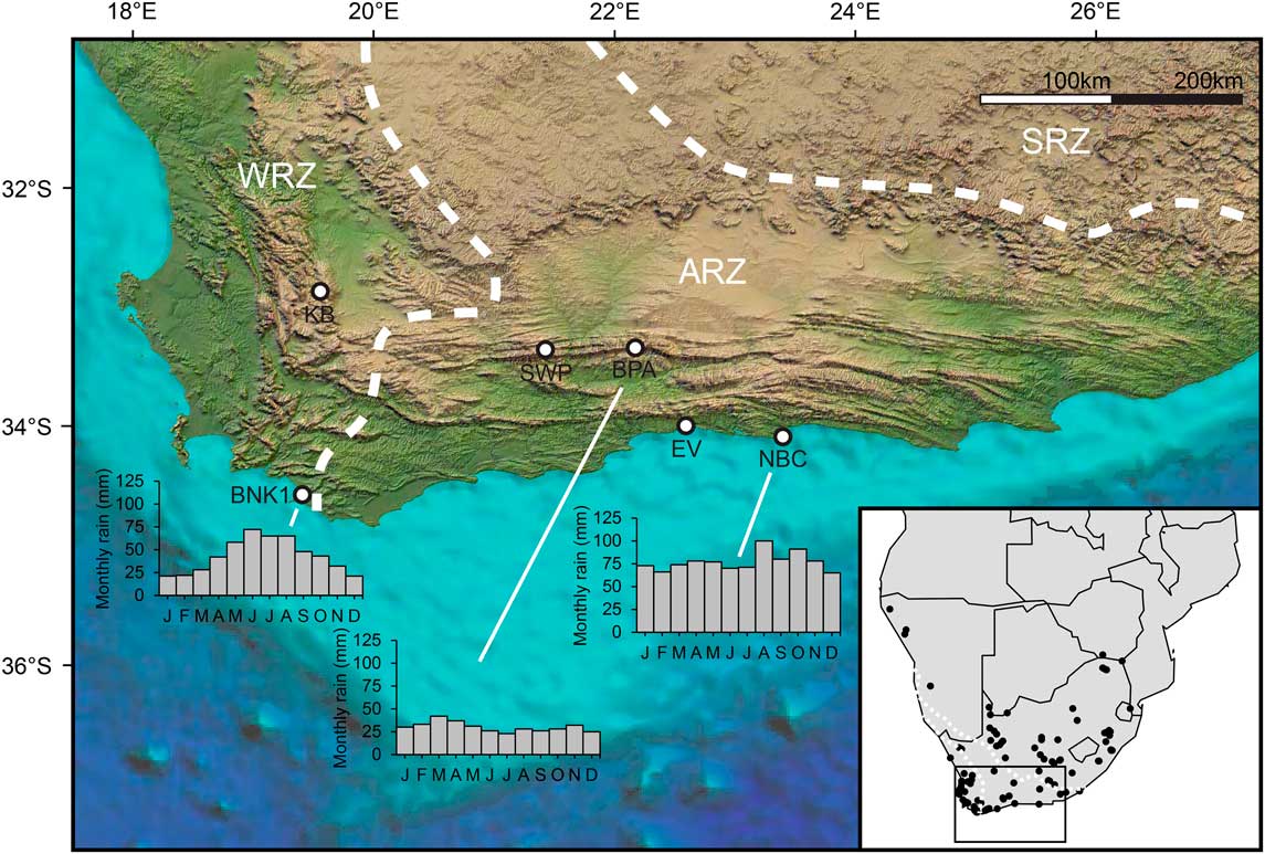
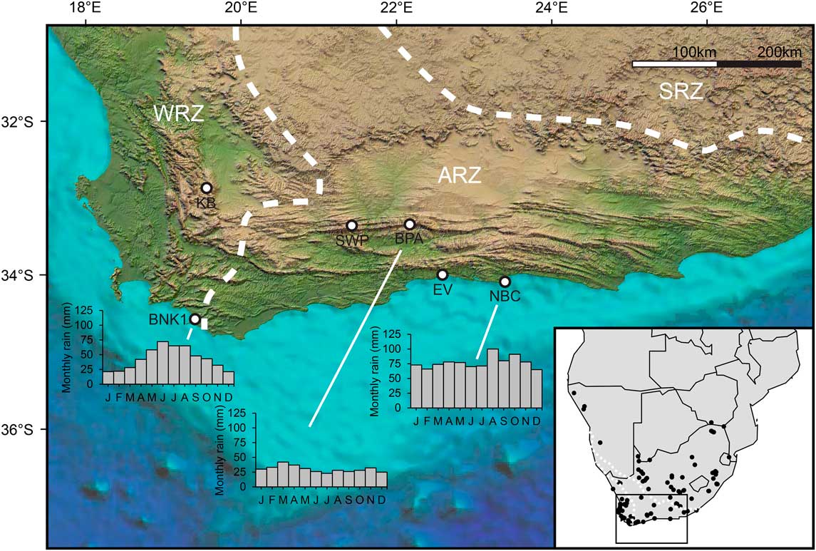
The southern Cape of South Africa, here defined as the region encompassing the southern coastal plains and the east–west trending ranges of the Cape Fold Belt, straddles the transition between the winter rainfall zone (WRZ; >66% of mean annual precipitation [MAP] falls from April to September) to the west and the summer rainfall zone (SRZ; >66% of MAP falls from October to March) to the east (sensu Chase and Meadows, Reference Chase and Meadows2007; Fig. 1). The WRZ receives most of its rainfall from frontal systems associated with the westerly storm track, which migrates northward during the austral winter. In contrast, precipitation in the SRZ is related to tropical easterly flow, which advects moisture from the Indian Ocean during the summer months (Tyson, Reference Tyson1986; Chase and Meadows, Reference Chase and Meadows2007). Because most of the southern Cape falls within the aseasonal rainfall zone (ARZ; Fig. 1), receiving precipitation throughout the year from both sources and their combined effects (Chase et al., Reference Chase, Chevalier, Boom and Carr2017, Reference Chase, Faith, Mackay, Chevalier, Carr, Boom, Lim and Reimer2018), the region is uniquely positioned to inform on the history of these temperate and tropical circulation systems.
(color online) The location of the three fossil sites examined here, with monthly rainfall totals (data from Hijmans et al. Reference Hijmans, Cameron, Parra, Jones and Jarvis2005), and other sites discussed in the text. BNK1, Byneskranskop 1; BPA, Boomplaas Cave; EV, Eilandvlei; KB, Katbakkies Pass; NBC, Nelson Bay Cave; SWP, Seweweekspoort. Inset: The location of 123 modern microfaunal samples across southern Africa. Dashed white lines denote boundaries of winter rainfall zone (WRZ), aseasonal rainfall zone (ARZ), and summer rainfall zone (SRZ).
Quaternary variability in these two systems in southern Africa has been a focus of research for decades (van Zinderen Bakker, Reference van Zinderen Bakker1967, Reference van Zinderen Bakker1976; Heine, Reference Heine1982; Cockcroft et al., Reference Cockcroft, Wilkinson and Tyson1987; Deacon and Lancaster, Reference Deacon and Lancaster1988). The dominant paradigm suggests that the boundaries of the WRZ and SRZ may have shifted through time because of the enhancement of winter rainfall during glacial periods and enhancement of summer rainfall during interglacial periods (see reviews in Deacon and Lancaster, Reference Deacon and Lancaster1988; Partridge et al., Reference Partridge, Avery, Botha, Brink, Deacon, Herbert and Maud1990; Chase and Meadows, Reference Chase and Meadows2007; Chase et al., Reference Chase, Chevalier, Boom and Carr2017). However, the precipitation history of the southern Cape remains unclear and debated. For instance, cool phases of the Pleistocene have been associated with enhanced winter rains (Faith, Reference Faith2013b; Sealy et al., Reference Sealy, Lee-Thorp, Loftus, Faith and Marean2016; Chase et al., Reference Chase, Faith, Mackay, Chevalier, Carr, Boom, Lim and Reimer2018), whereas some records link cool conditions to intensified summer rains (Bar-Matthews et al., Reference Bar-Matthews, Marean, Jacobs, Karkanas, Fisher, Herries and Brown2010). Even the most basic particulars—were glacial periods wetter or drier than interglacial periods?—are uncertain (Chase and Meadows, Reference Chase and Meadows2007; Marean et al., Reference Marean, Cawthra, Cowling, Esler, Fisher, Milewski, Potts, Singels and De Vynck2014), with some, for example, characterizing the last glacial maximum (LGM: 26.5–19 ka; Clark et al., Reference Clark, Dyke, Shakun, Carlson, Clark, Wohlfarth, Mitrovica, Hostetler and McCabe2009) as harsh and arid (e.g., Avery, Reference Avery1982; Deacon et al., Reference Deacon, Deacon, Scholtz, Thackeray and Brink1984; Deacon and Lancaster, Reference Deacon and Lancaster1988) or humid and highly productive (e.g., Faith, Reference Faith2013b; Chase et al., Reference Chase, Chevalier, Boom and Carr2017, Reference Chase, Faith, Mackay, Chevalier, Carr, Boom, Lim and Reimer2018). Uncertainty in these and other aspects of the region’s precipitation history stems in part from a lack of records that inform directly on the relevant climate parameters (Chase et al., Reference Chase, Boom, Carr, Meadows and Reimer2013). This is exacerbated by a combination of seemingly contradictory lines of evidence (e.g., Avery, Reference Avery1982, Reference Avery2004), conflicting interpretations of the evidence (e.g., Deacon et al., Reference Deacon, Deacon, Scholtz, Thackeray and Brink1984; Faith, Reference Faith2013a), and a substantial degree of not yet well-understood spatial variation (Chase et al., Reference Chase, Lim, Chevalier, Boom, Carr, Meadows and Reimer2015b, Reference Chase, Chevalier, Boom and Carr2017), such as evidence indicating that coastal archives are out of phase with those found in the interior (Chase and Quick, Reference Chase and Quick2018).
Of the various proxy records from the southern Cape (reviewed in Chase and Meadows, Reference Chase and Meadows2007; Marean et al., Reference Marean, Cawthra, Cowling, Esler, Fisher, Milewski, Potts, Singels and De Vynck2014), the fossil record of raptor-accumulated micromammal assemblages from cave deposits features prominently in discussion of past climate and environment (e.g., Avery, Reference Avery1982, Reference Avery1983, Reference Avery1987, Reference Avery1990, Reference Avery1993, Reference Avery2004; Deacon et al., Reference Deacon, Deacon, Scholtz, Thackeray and Brink1984; Thackeray, Reference Thackeray1987, Reference Thackeray1990; Matthews et al., Reference Matthews, Rector, Jacobs, Herries and Marean2011; Nel and Henshilwood, Reference Nel and Henshilwood2016; Thackeray and Fitchett, Reference Thackeray and Fitchett2016; Nel et al., Reference Nel, Wurz and Henshilwood2018). Such assemblages are widely used to inform on climate in a diverse range of geographic and temporal settings (e.g., Andrews, Reference Andrews1990), though interpretations of those from the southern Cape are, like other records from the region, not always in agreement (e.g., Avery, Reference Avery1982, Reference Avery2004; Thackeray, Reference Thackeray1987; Faith, Reference Faith2013a). Our aim here is to revisit several key late Quaternary micromammal sequences, with a focus on their implications for the region’s precipitation history. The main contribution of this study is that our interpretations are informed by a large sample of modern micromammal assemblages from southern Africa. We use these assemblages to relate variation in taxonomic composition to variation in climate, which provides an empirical framework for interpreting taxonomic fluctuations in the past.
MATERIALS AND METHODS
Micromammal assemblages
Our analysis makes use of taxonomic abundance data—quantified according to the minimum number of individuals (MNI) after Avery (Reference Avery1982)—from modern and fossil micromammal assemblages. The species included in our analysis typically weigh less than 150 g and include rodents (Rodentia), shrews (Soricidae), elephant shrews (Macroscelididae), and golden moles (Chrysochloridae). The taxonomy used here follows Wilson and Reeder (Reference Wilson and Reeder2005). Bats (Chiroptera) are not considered in our analysis.
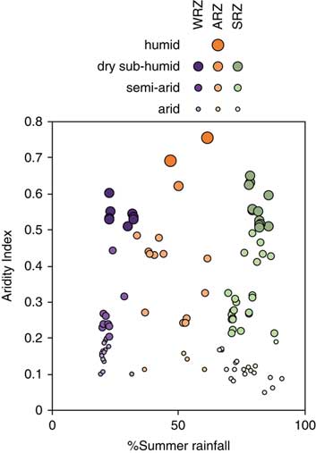
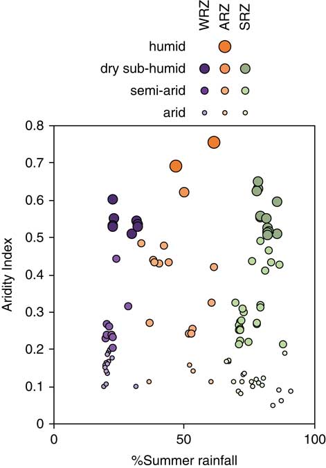
The modern sample includes 123 assemblages collected from barn owl (Tyto alba) roosts across southern Africa (Fig. 1) (see Avery, Reference Avery1999) and currently curated at the Iziko South African Museum in Cape Town (Supplementary Tables 1–2). At each sample locality, whole or partial barn owl pellets were collected, and, where appropriate, bulk debris from collapsed pellets was bagged for subsequent analysis. Some assemblages, such as those from West Coast National Park (Avery, Reference Avery1992), were sampled multiple times; they are analyzed here as a single aggregate. Assemblage sample size ranges from 24 to 6943 individuals (median = 243.5). Important to our work here, these assemblages encompass a broad range of precipitation regimes (from 19% to 91% summer rain), occurring in the SRZ (n = 60), the WRZ (n = 41), and the ARZ (n = 22). Following the United Nations Environment Programme (UNEP, 1997) classification scheme for aridity, sites are characterized by climates that are arid (n = 41), semiarid (n = 52), dry subhumid (n = 28), and humid (n = 2) (Fig. 2). We caution that the small sample of assemblages from humid climates limits our ability to model the relationship between species composition and climate at the more humid end of the spectrum.
(color online) The percentage of summer rainfall (% of rainfall from October to March) and aridity index (AI) values (= MAP/MAE, where MAP is mean annual precipitation and MAE is mean annual evapotranspiration; from Zomer et al., Reference Zomer, Bossio, Trabucco, Yuanjie, Gupta and Singh2007, Reference Zomer, Trabucco, Bossio, van Straaten and Verchot2008; Trabucco and Zomer, Reference Trabucco and Zomer2009) of the 123 modern microfauna samples. Higher AI values indicate more humid conditions. Humid = AI >0.65; dry subhumid = 0.5< AI <0.65; semiarid = 0.2< AI <0.5; arid = 0.05< AI <0.2. ARZ, aseasonal rainfall zone; SRZ, summer rainfall zone; WRZ, winter rainfall zone.
Fossil data are derived from Avery (Reference Avery1982) and include the late Quaternary assemblages from three southern Cape archaeological sites: Boomplaas Cave (Deacon, Reference Deacon1979) and Nelson Bay Cave (Klein, Reference Klein1972; Deacon, Reference Deacon1984) in the ARZ and Byneskranskop 1 (Schweitzer and Wilson, Reference Schweitzer and Wilson1982) in the WRZ (Fig. 1). These sites were selected to the exclusion of a few others from the region (e.g., Die Kelders and Klasies River) because of their more robust chronologies (Loftus et al., Reference Loftus, Sealy and Lee-Thorp2016; Pargeter et al., Reference Pargeter, Loftus, Mackay, Mitchell and Stewart2018), and because they include deposits sampling the transition from glacial to interglacial conditions. Located on the southern flanks of the Swartberg range ∼80 km inland, Boomplaas Cave was excavated by Hilary Deacon in the 1970s (Deacon, Reference Deacon1979, Reference Deacon1984). It provides the longest sequence examined here, spanning the last ∼65 ka, with a particularly well-dated sequence after the onset of the LGM (Pargeter et al., Reference Pargeter, Loftus, Mackay, Mitchell and Stewart2018). Nelson Bay Cave is located on the Robberg Peninsula on the southern Cape coastline. It was excavated by Ray Inskeep (Inskeep, Reference Inskeep1987) and later by Richard Klein (Klein, Reference Klein1972; see also Deacon, Reference Deacon1984). Microfauna data are only available from layers YSL and YGL (Klein’s excavation), dating to 23.5–21.0 ka and 22.1–16.3 ka, respectively (Loftus et al., Reference Loftus, Sealy and Lee-Thorp2016). Finally, Byneskranskop 1 is located at the western margin of the southern Cape, ∼7 km from the modern coastline. Excavations by Franz Schweitzer in the 1970s (Schweitzer and Wilson, Reference Schweitzer and Wilson1982) uncovered a stratified sequence spanning the last 17 ka (Loftus et al., Reference Loftus, Sealy and Lee-Thorp2016). The stratigraphy, chronology, and taxonomic abundance data for each of the assemblages examined here are reported in Supplementary Table 3.
Details concerning the taphonomic histories of the fossil assemblages require that some assumptions be made. First, we note that the microfauna from Boomplaas Cave were recovered using a combination of 2 and 3 mm mesh, whereas 3 mm mesh was used for the other two sites. Because finer mesh was not used at any site, there is potential for taphonomic bias against recovery of smaller specimens and smaller-bodied species (e.g., Lyman, Reference Lyman2012). We assume that the effects of such bias are consistent within a given site. In addition, assumptions are also made regarding the accumulator(s) of the micromammal remains. Avery (Reference Avery1982) argued that barn owls were the primary accumulators of the microfauna from all three sites. This inference was based on assessment of the ecology of potential accumulators and the represented prey species, as her analysis was conducted before development of taphonomic approaches for identifying the likely bone accumulators (e.g., Andrews, Reference Andrews1990). However, there is reason to believe that other raptor species could have accumulated some of the microfaunal remains examined here. For example, taphonomic analysis of the macrofauna from Boomplaas Cave indicates that some of the smaller species (e.g., leporids, hyraxes [Procavia capensis], smaller ungulates) were accumulated by very large raptors (Faith, Reference Faith2013a). Likewise, spotted eagle owls (Bubo africanus) are implicated in the taphonomic histories of other microfaunal assemblages from the region (Matthews et al., Reference Matthews, Rector, Jacobs, Herries and Marean2011; Nel et al., Reference Nel, Wurz and Henshilwood2018), though they generate microfaunal assemblages that are very similar in composition to those of barn owls (Reed, Reference Reed2005). In the absence of taphonomic analysis of the micromammal assemblages, we assume that contributions by other bone accumulators have not overprinted the environmental signal in a manner that would substantially alter our results.
Barn owl assemblages are usually thought to provide a reasonably accurate representation of the local micromammal community (e.g., Andrews, Reference Andrews1990; Fernández-Jalvo et al., Reference Fernández-Jalvo, Andrews, Denys, Sesé, Stoetzel, Marin-Monfort and Pesquero2016). They typically forage within a radius of up to 2–3 km (Andrews, Reference Andrews1990), preferentially targeting open habitats where it is easier to locate and capture prey (Taylor, Reference Taylor1994). The relatively small foraging radius implies that the modern and fossil assemblages examined here provide localized samples of the micromammal community. It follows that they may be especially sensitive to local environmental conditions. This spatial scale must be considered when interpreting micromammal assemblages in terms of much larger-scale climate phenomena (see “Discussion”). The open-habitat bias is less of a concern here, as it is likely to be consistent across all assemblages.
Analytical methods
For each of the 123 modern micromammal assemblages, we extracted data on rainfall seasonality and aridity from the WorldClim global climate database (Hijmans et al., Reference Hijmans, Cameron, Parra, Jones and Jarvis2005) and from the Global Aridity Index database (Zomer et al., Reference Zomer, Bossio, Trabucco, Yuanjie, Gupta and Singh2007, Reference Zomer, Trabucco, Bossio, van Straaten and Verchot2008; Trabucco and Zomer, Reference Trabucco and Zomer2009). Though there is a recent update to WorldClim (WorldClim 2: Fick and Hijmans, Reference Fick and Hijmans2017), we use the original because it provides the basis for the data modeled in the Global Aridity Index database. We calculated three complementary measures of rainfall seasonality from the WorldClim database: the percentage of annual precipitation that falls (1) during the coolest quarter of the year (% cold-quarter rainfall: June, July, August), (2) during the warmest quarter of the year (% warm-quarter rainfall: December, January, February), and (3) during the warmest half of the year (% summer rainfall: October through March). The aridity index (AI) reported in the Global Aridity Index database is expressed as
 $${\rm AI}{\equals}{\rm MAP}/{\rm MAE},$$
where MAP is mean annual precipitation and MAE is mean annual evapotranspiration. Higher AI values indicate more humid conditions. Although MAP is strongly correlated with AI in our data set (r = 0.958, P < 0.001), we focus on AI because many climate proxies, including flora and fauna, are more directly influenced by moisture availability (humidity/aridity) rather than the total amount of precipitation (e.g., Chevalier and Chase, Reference Chevalier and Chase2016). It is important to note, however, that although AI can be calculated at broad spatial scales, moisture availability is usually much more heterogeneous than these calculations suggest. Even modest topographic variability can significantly disperse or concentrate surface and groundwater resources, creating substantial microtopographic differences in moisture availability within regions of similar MAP/MAE.
We use canonical correspondence analysis (CCA) to relate the taxonomic composition of the modern assemblages to precipitation seasonality (% warm-quarter and % cold-quarter rainfall) and aridity. CCA is a constrained ordination approach in which faunal assemblages are ordinated relative to one or more known environmental variables, and the species abundances are considered a response to the environmental gradient (Legendre and Legendre, Reference Legendre and Legendre2012). When the primary axes are plotted in a bivariate plot, assemblages from similar climate regimes will plot close to each other, and the species will plot nearest to those assemblages in which they are most abundant. We then input the Quaternary fossil assemblages into the CCA as supplementary points; these are points that are projected in the same multivariate space as the modern assemblages, but they have no influence on the original ordination. Because the ordination of modern assemblages in the CCA is designed to track environmental variables (the extent to which this is so is examined subsequently), this allows us to interpret ordination scores of fossil assemblages in terms of precipitation seasonality and aridity. We exclude singleton taxa (i.e., those that occur in only one assemblage) from the analysis, as they can disproportionately influence the ordination (Legendre and Legendre, Reference Legendre and Legendre2012). All fossil assemblages with sample sizes greater than 10 individuals are included in the analysis (assemblage LOH from Boomplaas Cave and Layer 3 from Byneskranskop 1 are excluded).
The use of CCA allows us to consider the environmental implications of all taxa simultaneously, in contrast to traditional paleoenvironmental inferences derived from (potentially subjective) interpretations of a select handful of indicator taxa. Central to this approach is that the target variables (rainfall seasonality and aridity in the case of this study) must be important determinants of taxonomic composition (e.g., Birks, Reference Birks1995; Le and Shackleton, Reference Le and Shackleton1994). Though our primary interests concern aridity and rainfall seasonality, we recognize that the presence and abundance of a species in a given assemblage is likely mediated by multiple climatic or environmental variables. For example, some species may indicate local microenvironments (e.g., dense vegetation along a watercourse) irrespective of variation in our target environmental variables. In this study, we implemented a protocol to ensure analysis of those taxa that are relatively unambiguous indicators of rainfall seasonality or aridity. In particular, we eliminated taxa that are often found in both winter- or summer-dominated rainfall regimes and were not associated clearly with either relatively arid or humid climates. To do so, we calculated the interquartile range (IQR: 25th to 75th percentile) of % summer rainfall and AI values that characterize the modern assemblages in which a given taxon is found (see Supplemental Table 3). We excluded those taxa (n = 16) whose IQRs encompass intermediate values of rainfall seasonality and aridity, defined here as 50% summer rainfall and an AI value of 0.40; the former represents the threshold separating assemblages that receive more winter or more summer rainfall, and the latter represents the midpoint of the range of AI values in the modern sample (from 0.05 to 0.75). Not only are the excluded taxa ambiguous indicators of our target environmental variables (e.g., because they occur in humid and arid climates), but they also tend to have relatively broad tolerances with respect to rainfall seasonality and aridity. The median IQRs of % summer rainfall (46%) and AI values (0.29) of excluded taxa are considerably larger than those of taxa included in analysis (% summer rainfall: 16%; AI: 0.14). In other words, excluded taxa are found in modern assemblages characterized by a much broader range of seasonality and AI values than those retained for analysis.
Though it is possible to use these and related analytical approaches to generate numerical reconstructions of past climate (Birks, Reference Birks1995), we emphasize ordinal-scale trends here (e.g., more/less arid) to avoid generating results that imply an unwarranted degree of precision. There are several reasons for doing so. First, our assumptions concerning the taphonomic histories of the fossil assemblages reinforce the need for conservative interpretation of the fossil data. Second, taxonomic abundances from fossil mammal assemblages—typically quantified according to MNI or the number of identified specimens—often behave in a manner that is ordinal scale (Grayson, Reference Grayson1984; Lyman, Reference Lyman2008). Finally, we note that the analyzed fossil assemblages are time averaged by amounts ranging from hundreds to thousands of years. The precision implied by quantified paleoclimate reconstructions may be misleading considering that the relatively coarse temporal resolution of the fossil assemblages means they are sometimes poorly constrained chronologically and may reflect either short-term climatic fluctuations or the averaging of different discrete assemblages over longer time periods. It is for this reason—specifically, the need to ensure that we ask appropriate paleoclimatic questions that can be answered given the temporal resolution of the fossil data (e.g., Lyman, Reference Lyman2017)—that we also emphasize long-term paleoclimatic trends (e.g., from the LGM to the onset of the Holocene), highlighting shorter-term climate phenomena only when we have sufficient resolution to do so.
RESULTS
Modern assemblages
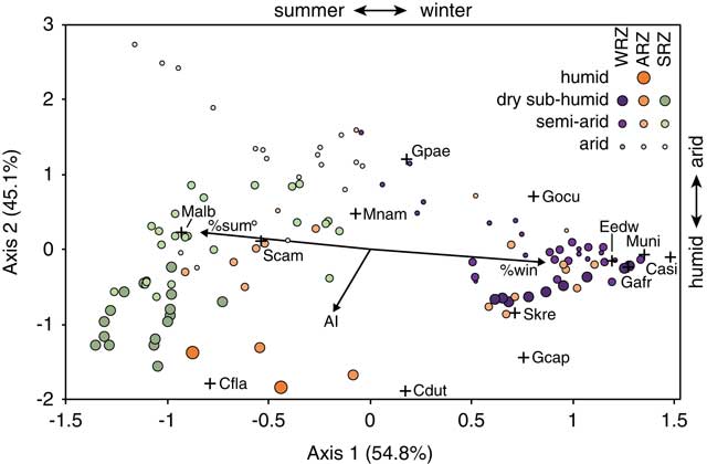
Figure 3 plots the ordination of sites and species along the first two axes of the CCA. For the sake of clarity, site names are omitted, and they are instead coded by precipitation regime (WRZ, SRZ, and ARZ) and UNEP aridity classification (arid, semiarid, dry subhumid, and humid). Only those species present in the fossil assemblages are illustrated here. Full details concerning the CCA ordination scores for sites and taxa are provided in Supplementary Table 4.
(color online) Ordination of modern assemblages (circles) and taxa (+) along the first two axes of the canonical correspondence analysis. Arrows indicate vectors for the aridity index (AI), % warm-quarter rainfall (% sum), and % cold-quarter rainfall (% win). For the sake of clarity, only those taxa occurring in the late Quaternary fossil samples are illustrated here (see Supplementary Table 4 for all taxa). Species abbreviations are as follows: Casi, Chrysochloris asiatica; Cdut, Chlorotalpa duthiae; Cfla, Crocidura flavescens; Eedw, Elephantulus edwardii; Gafr, Gerbilliscus afra; Gcap, Georychus capensis; Gocu, Graphiurus ocularis; Gpae, Gerbillurus paeba; Malb, Mystromys albicaudatus; Mnam, Micaleamys namaquensis; Muni, Myotomys unisulcatus; Scam, Saccostomus campestris; Skre, Steatomys krebsii. ARZ, aseasonal rainfall zone; SRZ, summer rainfall zone; WRZ, winter rainfall zone.
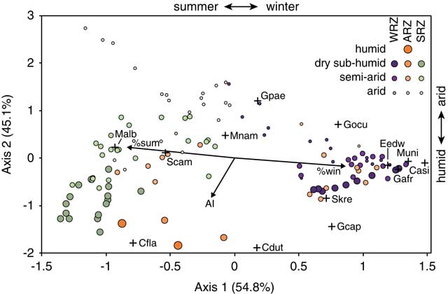
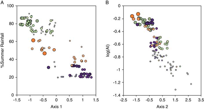
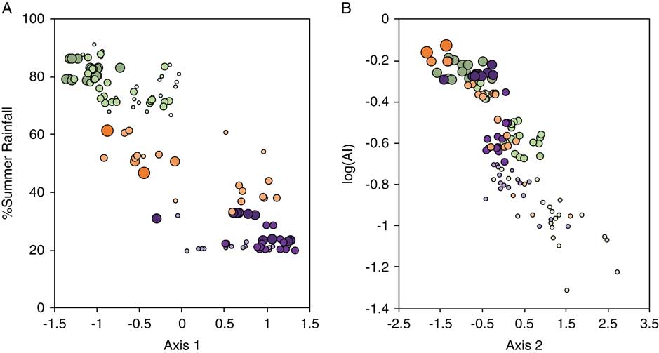
The first axis (axis 1) accounts for 54.8% of the inertia (∼variation in taxonomic composition), and it broadly tracks precipitation seasonality. Sites and species with negative values are associated with a greater percentage of warm-quarter rainfall, and those with positive values are associated with a greater percentage of cold-quarter rainfall. This relationship is further illustrated in Figure 4A, which plots the axis 1 scores for a given site against % summer rainfall. There is a strong and significant inverse correlation between the two variables (r = −0.880, P < 0.001). The second axis of the CCA accounts for 45.1% of the inertia and tracks the AI (Fig. 3). Sites and species associated with more humid environments tend to have negative axis 2 scores, whereas those associated with arid settings tend to have positive axis 2 scores. This is also shown in Figure 4B, which plots axis 2 scores against the logarithm of the AI. The correlation is strong and highly significant (r = −0.859, P < 0.001).
(color online) The relationship between axis 1 and the % summer rainfall (A) and the relationship between axis 2 and the logarithm of the aridity index (AI) (B) across the 123 modern microfaunal assemblages. Symbol legend for modern assemblages follows Figure 2.
Fossil assemblages
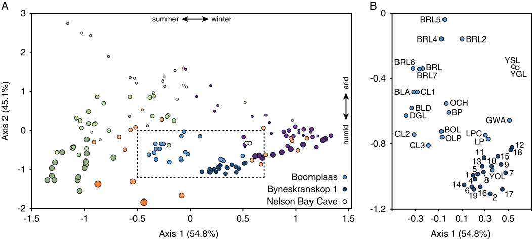
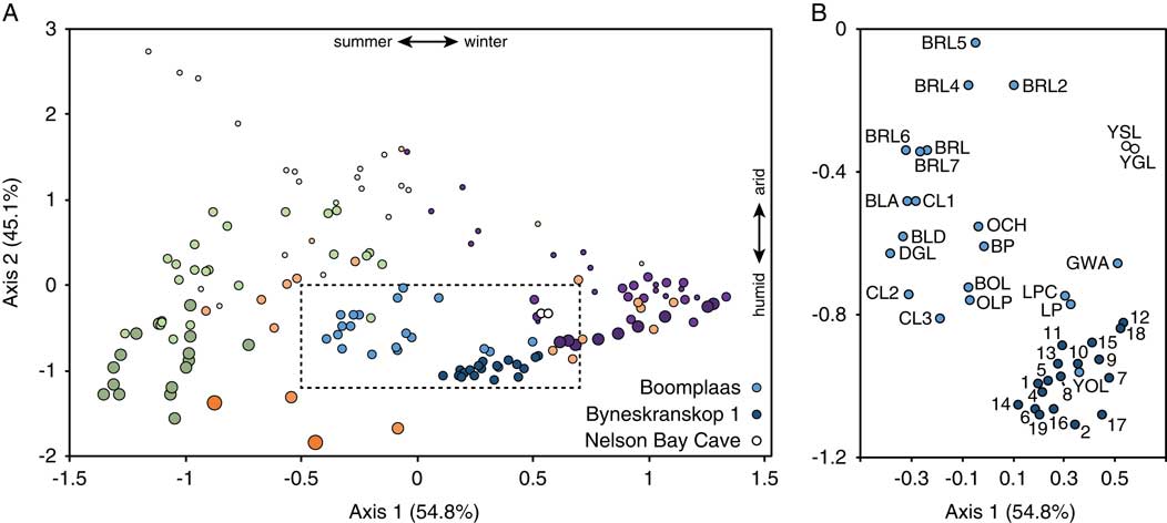
The previous analysis indicates that we can use the ordination of assemblages along the first two axes to track ordinal-scale change in rainfall seasonality and aridity in the fossil record. Figure 5 plots the fossil assemblages in the same multivariate space as the modern assemblages. Though sample size can potentially influence such analyses because larger samples translate to recovery of more species (Grayson, Reference Grayson1984; Lyman, Reference Lyman2008), which could potentially include species with a disproportionate effect on the ordination, this is not the case here; for the two sites with long stratified microfaunal sequences (Boomplaas and Byneskranskop 1), assemblage sample size is not related to axis 1 and 2 scores (Spearman’s rho: P >0.15 for all correlations).
(color online) (A) Ordination of fossil assemblages relative to the modern assemblages. Symbol legend for modern assemblages follows Figure 2. Box encompassing fossil assemblages shown in panel B, with modern assemblages removed for clarity.
Boomplaas Cave
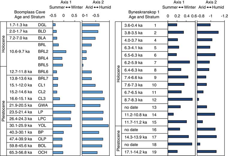
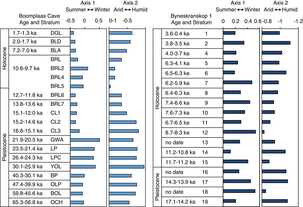
The Boomplaas Cave assemblages show substantial variation along both axes (Figs. 5–7). From the base of the sequence to the end of the LGM (layer GWA), increasing axis 1 scores suggests increasing winter rainfall (Spearman’s rho: r s = −0.857, P = 0.007). Axis 2 scores remain relatively low (= humid) and stable at this time. The last glacial-interglacial transition (LGIT: layers CL3 to BRL6) is associated with considerably lower axis 1 scores and a significant temporal increase in axis 2 scores (r s = 1.000, P = 0.017), suggesting enhanced summer rainfall and increasing aridity relative to the LGM. The shift toward more arid conditions peaks in the earliest Holocene (BRL5), with conditions becoming more humid thereafter (declining axis 2 scores from BRL5 to DGL: r s = –1.000, P < 0.001). The increase in humidity through the Holocene is associated with increased influence of summer rains (declining axis 1 scores from BRL5 to DGL: r s = –0.893, P = 0.012).
(color online) Axis 1 (rainfall seasonality) and axis 2 (aridity) scores through the Boomplaas Cave and Byneskranskop 1 sequences. Ages for CL3 and up represent calibrated 2σ ranges of all 14C ages in a given stratum, using SHCal13 (Hogg et al., Reference Hogg, Hua, Blackwell, Niu, Buck, Guilderson and Heaton2013) calibration data and OxCal 4.3 (Bronk Ramsey, Reference Bronk Ramsey2009, Reference Bronk Ramsey2013). Ages for GWA and below are modeled age estimates from Pargeter et al. (Reference Pargeter, Loftus, Mackay, Mitchell and Stewart2018).
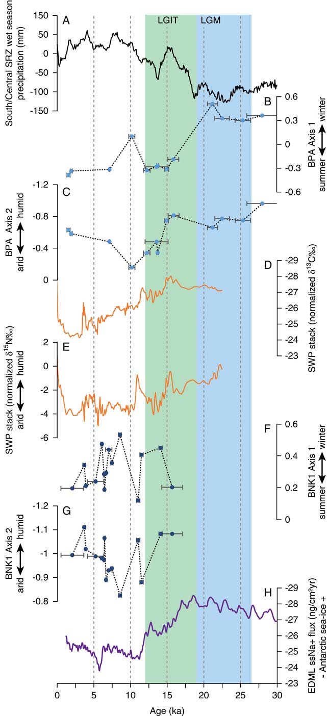
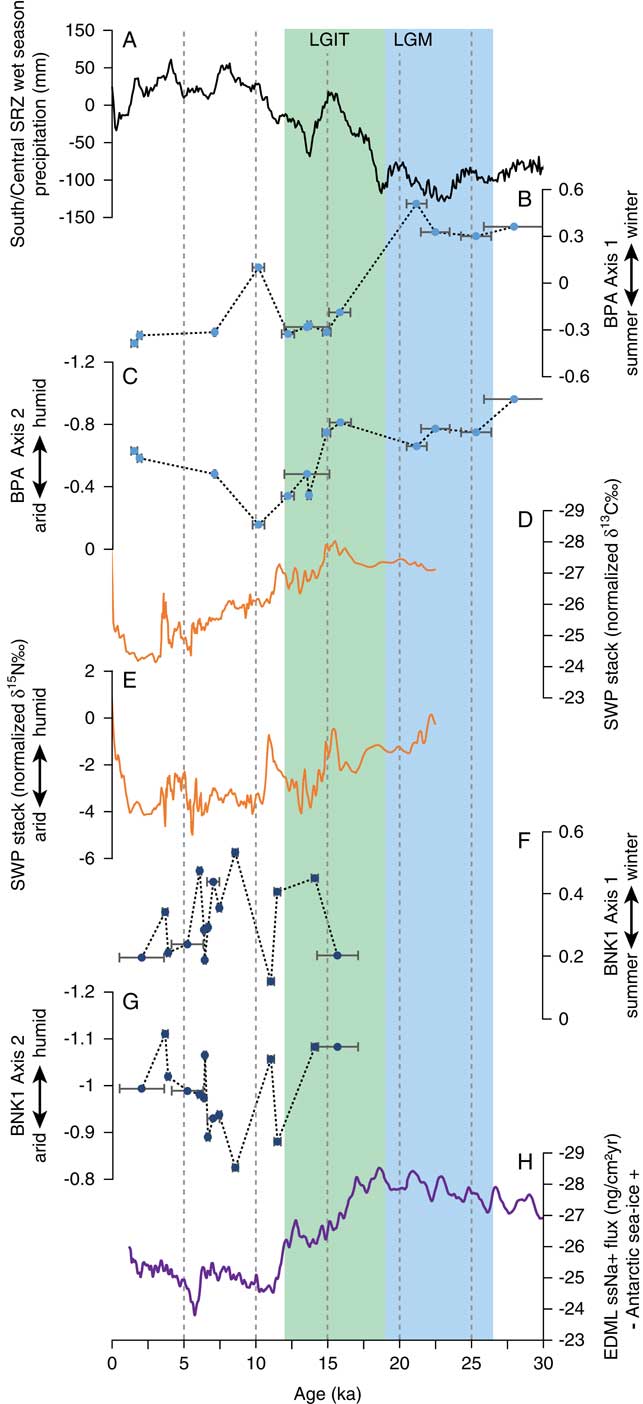
(color online) Comparison of precipitation seasonality (axis 1) and aridity (axis 2) reconstructions from Boomplaas Cave (BPA; B, C) and Byneskranskop 1 (BNK1; F, G) to local and regional proxy records, including southern-central summer rainfall zone (SRZ) wet season precipitation (Chevalier and Chase, Reference Chevalier and Chase2015) (A), δ13C (D) and δ15N (E) stacks from the Seweweekspoort hyrax middens (Chase et al. Reference Chase, Chevalier, Boom and Carr2017, Reference Chase, Faith, Mackay, Chevalier, Carr, Boom, Lim and Reimer2018), and sea-salt sodium flux from the EDML ice core indicating Antarctic sea-ice extent (Fischer et al., Reference Fischer, Fundel, Ruth, Twarloh, Wegner, Udisti and Becagli2007) (H). Undated fossil assemblages are not plotted here. Error bars for microfauna assemblages correspond to age ranges reported in Figure 6. BNK1, Byneskranskop 1; BPA, Boomplaas Cave; EDML, EPICA (European Project for Ice Coring in Antarctica) drill sites in Dronning Maud Land; LGIT, last glacial-interglacial transition; LGM, last glacial maximum; SRZ, summer rainfall zone; SWP, Seweweekspoort.
Nelson Bay Cave
The availability of only two assemblages from Nelson Bay Cave precludes an analysis of temporal change, but they do speak to LGM conditions on the south coastal plains—though the coastline was far from the site at this time (Van Andel, Reference Van Andel1989; Fisher et al., Reference Fisher, Bar-Matthews, Jerardino and Marean2010)—relative to the other fossil samples. As indicated in Figure 5, both assemblages from this site have positive axis 1 scores that are comparable to or greater than the LGM assemblages from Boomplaas and those from Byneskranskop 1. Though we lack a Holocene comparison from Nelson Bay Cave, this is consistent with enhanced winter rains during the LGM, especially considering the similarities in axis 1 scores with a south coast site that is today in the WRZ (Byneskranskop 1). The axis 2 scores are more positive than those from the LGM at Boomplaas Cave, implying drier conditions on the south coastal plains relative to the Swartberg range.
Byneskranskop 1
The Byneskranskop 1 assemblages show relatively muted variation along the first and second axes of the CCA (Figs. 5–7). There are no clear directional changes across the LGIT (layers 19–15; Fig. 6), though there is considerable variation within the Holocene (Figs. 6, 7). This variation includes a brief humid pulse associated with increased influence of summer rainfall in the earliest Holocene (layer 14: ∼11 cal ka BP), followed by the most arid and winter rainfall-dominated portion of the sequence in layer 12 (∼8.5 cal ka BP) (Figs. 6, 7). We also observe a steady and statistically significant increase in humidity (declining axis 2 scores: r s = –0.900, P < 0.001) coupled with increasing summer rainfall (declining axis 1 scores: r s = –0.636, P = 0.032) from layer 12 through to the top of the sequence. To the extent that the uppermost assemblage signals climates similar to the present, we infer that the influence of summer rainfall has been similar to or less than today, implying dominance of winter rainfall throughout the last 17 ka.
DISCUSSION
Our analyses differ from previous studies of southern Cape micromammal assemblages in that they are informed by a large sample of modern assemblages, which provides an empirical link between taxonomic composition and climate (see also Campbell et al., Reference Campbell, Lewis and Williams2011, Reference Campbell, Lewis, Thies and Williams2012). The strong relationships between taxonomic composition and climate documented in our analysis (Fig. 4) enhance confidence that our interpretations of the fossil record are reflecting changes in the target environmental variables. Particularly important are the high coefficients of determination (r 2) for the correlations involving rainfall seasonality (axis 1 and % summer rainfall: r 2 = 0.775) and aridity (axis 2 and AI: r 2 = 0.738), which together imply that the majority of variance in taxonomic composition of the modern assemblages is related to the target climatic variables. It follows that even though barn owl assemblages provide local representations of the micromammal community (within a 2–3 km radius), they are still highly sensitive to larger-scale climate phenomena, at least over the spatial scales examined here. Though the microfaunal record is not as well resolved as some other climate records from the region—namely, those provided by hyrax middens (e.g., Chase et al., Reference Chase, Lim, Chevalier, Boom, Carr, Meadows and Reimer2015b, Reference Chase, Faith, Mackay, Chevalier, Carr, Boom, Lim and Reimer2018), speleothems (e.g., Talma and Vogel, Reference Talma and Vogel1992), and lake cores (e.g., Quick et al., Reference Quick, Carr, Meadows, Boom, Bateman, Roberts, Reimer and Chase2015, Reference Quick, Meadows, Bateman, Kirsten, Mäusbacher, Haberzettle and Chase2016)—it does provide a valuable, and compared with many archives, unique, opportunity to simultaneously explore shifts in both moisture availability and rainfall seasonality.
Change in the ARZ
The Boomplaas Cave record contributes to an increasingly coherent picture concerning late Quaternary variation in temperate (winter rains) and tropical (summer rains) precipitation systems in what is today the ARZ. It attests to increasing influence of winter rains after ∼60 ka, with the strongest winter rainfall signal occurring immediately before and during the LGM (Fig. 6). The Nelson Bay Cave record is consistent with this trend, providing a strong winter rainfall signal in the two samples dating from 23.5 to 16.3 cal ka BP (Fig. 5).
Enhanced winter rains during the LGM are consistent with recent inferences derived from the Boomplaas microfauna (Thackeray and Fitchett, Reference Thackeray and Fitchett2016) and with stable carbon (δ13C) isotopes from Boomplaas grazers (Sealy et al., Reference Sealy, Lee-Thorp, Loftus, Faith and Marean2016). The latter indicate abundant C3 grass during the LGM; because the proportion of C3 and C4 grasses in South Africa tracks the influence of winter and summer rains (Vogel et al., Reference Vogel, Fuls and Ellis1978), this is consistent with greater influence of winter rainfall. Likewise, the expansion of grassland implied by the Boomplaas micromammals (Avery, Reference Avery1982) and larger mammals (Klein, Reference Klein1983; Faith, Reference Faith2013a), together with the strong C3 signature in the nearby (∼3 km east) Cango Caves speleothem (Talma and Vogel, Reference Talma and Vogel1992), is also indicative of abundant C3 grasses and winter rains at this time. Further afield at Seweweeksport, in the Swartberg range 70 km west of Boomplaas (Fig. 1), the combination of elevated grass pollen and reduced δ13C in a series of hyrax middens suggests that most rain fell during the winter (Chase et al., Reference Chase, Chevalier, Boom and Carr2017, Reference Chase, Faith, Mackay, Chevalier, Carr, Boom, Lim and Reimer2018) (Fig. 7D). A potential discrepancy is provided by Sealy’s (Reference Sealy1996) analysis of δ13C in grazers from Nelson Bay Cave. She interpreted stasis in the δ13C values of Syncerus caffer and Hippotragus spp. through the sequence as evidence for stability in the influence of summer and winter rainfall regimes. However, we note that this signal may be influenced by east–west migration of ungulate grazers along the paleo-Agulhas plain during the LGM (Marean, Reference Marean2010; Faith and Thompson, Reference Faith and Thompson2013; Copeland et al., Reference Copeland, Cawthra, Fisher, Lee-Thorp, Cowling, le Roux, Hodgkins and Marean2016), which would imply that their δ13C signatures are not indicative of local vegetation or rainfall regimes. Further, studies of Holocene climate change in the southern Cape have also highlighted that coastal sites may exhibit distinct, and even opposing, climate signals when compared with sites from the Swartberg and continental interior (Chase and Quick, Reference Chase and Quick2018). It is possible that apparent conflicts between records from the coastal plains and interior sites during the late Pleistocene reflect similar climatic gradients, but until more comparable data are obtained, this will remain an open question.
At Boomplaas Cave, the LGIT (CL3 to BRL6) is associated with enhanced summer rainfall relative to the LGM (Fig. 6). This is also evident in the Seweweekspoort δ13C record, which documents an increase in C4 vegetation through the LGIT (Fig. 7D). The increasing influence of summer rains broadly tracks changes in summer rainfall inferred from a recent statistical analysis of pollen archives in the interior (SRZ) of southern Africa (Chevalier and Chase, Reference Chevalier and Chase2015) (Fig. 7A). At the same time, the declining influence of winter rains also tracks the decline in Antarctic sea-ice extent inferred from sea-salt sodium flux from the EDML (EPICA [European Project for Ice Coring in Antarctica] drill sites in Dronning Maud Land) ice core (Fischer et al., Reference Fischer, Fundel, Ruth, Twarloh, Wegner, Udisti and Becagli2007; Fig. 7H), consistent with the hypothesis that winter rains are linked to the expansion and contraction of Antarctic sea ice and its effect on the position of the southern westerlies (e.g., van Zinderen Bakker, Reference van Zinderen Bakker1976; Stuut et al., Reference Stuut, Crosta, van der Borg and Schneider2004; Chase and Meadows, Reference Chase and Meadows2007; Chase et al., Reference Chase, Boom, Carr, Meadows and Reimer2013, Reference Chase, Chevalier, Boom and Carr2017).
In contrast to the coherent picture concerning rainfall seasonality provided by southern Cape paleoclimate archives, there is substantial disagreement about variation in moisture availability from the ARZ (e.g., Avery, Reference Avery1982, Reference Avery2004; Deacon et al., Reference Deacon, Deacon, Scholtz, Thackeray and Brink1984; Scholtz, Reference Scholtz1986; Deacon and Lancaster, Reference Deacon and Lancaster1988; Chase and Meadows, Reference Chase and Meadows2007; Faith, Reference Faith2013a, Reference Faith2013b; Chase et al., Reference Chase, Chevalier, Boom and Carr2017, Reference Chase, Faith, Mackay, Chevalier, Carr, Boom, Lim and Reimer2018). Our results contribute to a growing body of evidence suggesting a transition from a relatively humid LGM to a more arid Holocene (e.g., Faith Reference Faith2013a, Reference Faith2013b; Chase et al., Reference Chase, Chevalier, Boom and Carr2017, Reference Chase, Faith, Mackay, Chevalier, Carr, Boom, Lim and Reimer2018). The increase in aridity from the LGM to the early Holocene at Boomplaas Cave (Fig. 7C) broadly parallels the δ15N record from the Seweweekspoort hyrax middens (Chase et al., Reference Chase, Chevalier, Boom and Carr2017, Reference Chase, Faith, Mackay, Chevalier, Carr, Boom, Lim and Reimer2018; Fig. 7E). These records are out of phase with the pollen-derived precipitation record from the SRZ (Chevalier and Chase, Reference Chevalier and Chase2015; Fig. 7A), consistent with the expected inverse relationship between temperate and tropical systems over orbital time scales (Chase et al., Reference Chase, Chevalier, Boom and Carr2017).
The relatively humid conditions observed during the LGM persist until ∼15 ka, with conditions becoming increasingly arid through the rest of the Pleistocene sequence (Figs. 6, 7C). Increasing aridity at the end of the Pleistocene (∼15–12 ka) corresponds with a phase of reduced precipitation in the SRZ (Fig. 7A; Chevalier and Chase, Reference Chevalier and Chase2015) and a moderate decline in the extent of Antarctic sea ice (Fig. 7H). Together with relatively stability in rainfall seasonality at Boomplaas Cave (Fig. 7B), this suggests a decline in precipitation from both tropical and temperate systems, perhaps enhanced by increased evapotranspiration because of warming temperatures. The aridification trend peaks in the earliest Holocene (Figs. 6, 7C), which represents the most arid portion of the sequence. There is no evidence in the Boomplaas Cave record for the humid pulse seen at Seweweekspoort at ∼11 ka (Fig. 7E), but in the absence of better age control for the early Holocene portion of the sequence, we cannot rule out the possibility that Boomplaas lacks deposits that sample this relatively short-lived episode or that time averaging may have muted the signal.
The phase of early Holocene aridity documented in the micromammal record is followed by increasingly humid conditions coupled with a moderate increase in the proportion of summer rain (Fig. 6). The Seweweekspoort δ15N record does not indicate a comparable directional change in moisture availability, but it does indicate an increase in grass pollen (Chase et al., Reference Chase, Faith, Mackay, Chevalier, Carr, Boom, Lim and Reimer2018) in conjunction with a stronger C4 signature from the early Holocene until ∼2 ka (Fig. 7D). An increase in C4 grasses is also evident in the Cango Caves speleothem for the latter half of the Holocene (there is no record for the first half) (Talma and Vogel, Reference Talma and Vogel1992). The combination of evidence from these three archives implies enhanced summer rainfall in the region. Greater rainfall in the warmest portion of the year is likely to promote expansion of shallow-rooting vegetation, including C4 grasses. Why this increase in summer rainfall is apparently associated with greater humidity at Boomplaas but not at Seweweekspoort is not immediately clear. Resolving this discrepancy will require, among other things, additional records from the ARZ.
Change in the WRZ
The Byneskranskop 1 micromammals provide relatively little evidence for major changes in rainfall seasonality (e.g., compared with Boomplaas Cave), implying a dominance of winter rains over the last 17 ka (Fig. 6). This is not surprising given that the site is in the southwestern Cape and the core of the WRZ. In terms of both seasonality and aridity, there are no clear directional changes across the LGIT (layers 19–16: Fig. 6). Rather, changes within the Holocene (layers 15–1) are more pronounced than those occurring across the Pleistocene-Holocene transition. The earliest Holocene (layer 14) is associated with humid conditions (low axis 2 scores), corresponding closely with a similar humid pulse documented in the Seweweekspoort record (Chase et al., Reference Chase, Chevalier, Boom and Carr2017, Reference Chase, Faith, Mackay, Chevalier, Carr, Boom, Lim and Reimer2018), where it dates from 11.8 to 10.7 cal ka BP (Fig. 7E). The mechanisms underpinning this humid phase have been suggested to relate to an increase in tropical influence (Chase et al., Reference Chase, Chevalier, Boom and Carr2017), and this is clearly reflected in the micromammalian assemblage by reduced axis 1 scores (Figs. 6, 7).
Following the brief humid phase in the earliest Holocene, we observe a relatively arid terminal early Holocene/early to mid-Holocene transition—with the driest conditions occurring in layer 12 (8.7–8.3 cal ka BP)—followed by a gradual return to more humid conditions thereafter (Figs. 6, 7). This arid phase has been attributed to reduced influence of the westerlies (Chase et al., Reference Chase, Chevalier, Boom and Carr2017), and numerous records from elsewhere in the WRZ also suggest that at least parts the middle Holocene were more arid than the late Holocene (e.g., Klein, Reference Klein1991; Meadows et al., Reference Meadows, Baxter and Parkington1996; Meadows and Baxter, Reference Meadows and Baxter2001; Chase and Thomas, Reference Chase and Thomas2007; Scott and Woodborne, Reference Scott and Woodborne2007a, Reference Scott and Woodborne2007b; Klein and Cruz-Uribe, Reference Klein and Cruz-Uribe2016). Avery (Reference Avery1993) previously linked expansion of grasses during the mid-Holocene to a less seasonal rainfall regime (i.e., a greater proportion of summer rains), but this is not evident in our analysis, which implies that summer rains were relatively unimportant at this time (Fig. 7F). Though it has been suggested that cooler temperatures and increased westerly influence may account for the more humid late Holocene (e.g., Chase and Meadows, Reference Chase and Meadows2007), more recent evidence (Chase et al., Reference Chase, Chevalier, Boom and Carr2017) indicates a decrease in westerly influence and drier conditions at some WRZ sites (Chase et al., Reference Chase, Boom, Carr, Carré, Chevalier, Meadows, Pedro, Stager and Reimer2015a). At Byneskranskop 1, the shift toward mesic conditions after ∼8 ka (Fig. 7G) is associated with (slightly) greater influence of summer rainfall (Fig. 7F), potentially translating to a less severe summer drought. This is consistent with evidence and inferences drawn from hyrax midden data from the eastern WRZ at Katbakkies Pass (Fig. 1), which indicate that although most rain falls in the winter, variation in overall moisture availability/drought stress is largely determined by the changing influence of summer rains and their effect on the severity of the dry season (see Chase et al., Reference Chase, Lim, Chevalier, Boom, Carr, Meadows and Reimer2015b). The resolution and nature of the Byneskranskop 1 record makes direct comparison difficult, but the general trend of increasing humidity across the mid- to late Holocene is not inconsistent with results from Eilandvlei (250 km to the east in the Wilderness region), based on percentages of afrotemperate forest pollen (Quick et al., Reference Quick, Chase, Wündsch, Kirsten, Cheavlier, Mäusbacher, Meadows and Haberzettl2018). These similarities may be engendered by Byneskranskop 1’s near-coastal position, which may have been, relative to Boomplaas, more strongly influenced by the Agulhas Current and the transmission of tropical influences (Chase and Quick, Reference Chase and Quick2018).
CONCLUSIONS
We show that the taxonomic composition of southern African owl–accumulated micromammal assemblages is strongly related to precipitation seasonality and aridity. We use these relationships to infer changes in the late Quaternary precipitation history of the southern Cape from three fossil assemblages. In what is today the ARZ, the micromammal records from Boomplaas Cave and Nelson Bay Cave imply enhanced winter rainfall during glacial Pleistocene, consistent with models suggesting eastward expansion of the WRZ (e.g., van Zinderen Bakker, Reference van Zinderen Bakker1976; Chase and Meadows, Reference Chase and Meadows2007; Chase et al., Reference Chase, Chevalier, Boom and Carr2017). The Boomplaas Cave record contributes to a growing body of evidence implying a relatively humid LGM, followed by increased aridity across the LGIT. The WRZ record from Byneskranskop 1 is characterized by relatively little change in rainfall seasonality throughout its sequence. Changes in moisture availability are more pronounced, however, especially during the Holocene. This includes a period of aridity at the end of the early Holocene, followed by an increasingly humid middle to late Holocene, consistent with other records from the WRZ. Overall, the coherence between the micromammal record and other local and regional climate proxies (Fig. 7) reinforces the potential of southern African micromammal assemblages as indicators of paleoclimate (Avery, Reference Avery1983, Reference Avery1990, Reference Avery2007). Although new climate archives will be essential to resolving current and emerging questions concerning southern Africa’s precipitation history, our analyses show that new analysis of the existing records can also help to refine our understanding of environmental change.
ACKNOWLEDGMENTS
An early version of this study was presented at a Society for American Archaeology session organized by Eugene Morin, Arianne Boileau, and Elspeth Ready. The version reported here benefited from several participant comments. We thank the members of the University of Utah Archaeological Center, Curtis Marean (associate editor), and three anonymous referees for valuable feedback on an earlier draft. Justin Pargeter kindly shared new radiocarbon dates for Boomplaas Cave prior to their publication. An Australian Research Council Discovery Early Career Researcher Award (DE160100030) supported JTF in the early stages of this project.
SUPPLEMENTARY MATERIAL
To view supplementary material for this article, please visit https://doi.org/10.1017/qua.2018.105