1. Introduction
Landslides, debris flows and avalanches are known to alter their volumes by entraining and detraining material at their base (Chen, Crosta & Lee Reference Chen, Crosta and Lee2006; Mangeney et al. Reference Mangeney, Roche, Hungr, Mangold, Faccanoni and Lucas2010; Iverson Reference Iverson2012). Flow therefore occurs between two evolving boundaries: the top free surface and a basal yield surface across which material transfer takes place. The problem is then to model the mutual dependence between basal entrainment and the dynamics of the flow. In the present work, we pursue this issue for the simplest case of dense dry granular flows between smooth parallel walls. For this case, evolving interfaces between static and flowing grains can be observed in a variety of simple experimental configurations. These include avalanching flows in rotating drums (Gray Reference Gray2001), granular flows down inclined heaps (Taberlet et al. Reference Taberlet, Richard, Valance, Losert, Pasini, Jenkins and Delannay2003; Jop, Forterre & Pouliquen Reference Jop, Forterre and Pouliquen2005) and surges resulting from column collapse (Lube et al. Reference Lube, Huppert, Sparks and Freundt2007).
For shallow water and shallow granular flows over rigid beds, great simplifications result from using depth-integrated equations expressing mass and momentum balance (Savage & Hutter Reference Savage and Hutter1991; Liggett Reference Liggett1994). We therefore aim to extend this approach to entraining granular flows. Unlike previous efforts (Tai & Kuo Reference Tai and Kuo2008; Lê & Pitman Reference Lê and Pitman2010; Iverson Reference Iverson2012), we wish to avoid prescribing an extra closure relation for the erosion rate. Instead, we want to rely only on assumptions regarding the granular stresses. The behaviour and role of these stresses have been greatly clarified in recent years. Particle simulations (da Cruz et al. Reference da Cruz, Emam, Prochnow, Roux and Chevoir2005) and experiments (Jop et al. Reference Jop, Forterre and Pouliquen2005; Jop, Forterre & Pouliquen Reference Jop, Forterre and Pouliquen2007) have shown that the internal stresses in dense dry granular flows can be approximated by a simple viscoplastic rheology, with pressure-dependent yield stress and effective viscosity. In channels of finite width, experiments have also highlighted the crucial role of friction along the sidewalls (Taberlet et al. Reference Taberlet, Richard, Valance, Losert, Pasini, Jenkins and Delannay2003; Jop et al. Reference Jop, Forterre and Pouliquen2005). Numerical simulations (Jop et al. Reference Jop, Forterre and Pouliquen2007; Lagrée, Staron & Popinet Reference Lagrée, Staron and Popinet2011; Ionescu et al. Reference Ionescu, Mangeney, Bouchut and Roche2014) indicate that these ingredients suffice to capture evolving transitions between static and flowing grains. In principle, therefore, no extra erosion law should be needed.
To model entraining flows without prescribing erosion rates, we propose to complement the mass and momentum equations with an additional depth-integrated equation expressing the balance of kinetic energy. Similar strategies balancing higher moments of the velocity profile were earlier applied to sheared shallow water flows by Steffler & Jin (Reference Steffler and Jin1993) and Richard & Gavrilyuk (Reference Richard and Gavrilyuk2013). In § 2, we first derive the equations in the general context of unsteady spatially varied flows. In § 3, we then apply the equations to transient heap flows. These are unsteady but longitudinally uniform flows for which the equations reduce to a pair of ordinary differential equations (ODEs). To check that depth integration does not cause a significant loss of information, we compare the results with numerical solutions of the full local equations. Comparisons with transient heap flow experiments are presented in § 4.
2. Theory
2.1. Local equations, constitutive relations and boundary conditions
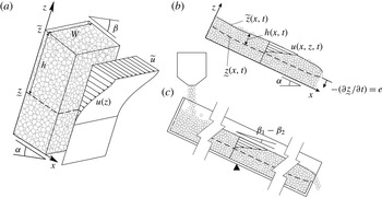
Channelized granular flows over erodible beds: (a) variable definitions and velocity distribution for a typical granular column; (b) evolving profiles for a generic space- and time-varying flow; (c) the seesaw channel configuration used to produce transient uniform flows.

In an open channel of constant width
 $W$
, we consider a dense flow of dry grains over an erodible granular substrate (figure 1
a). At a given location
 $x$
and time
 $t$
, grains move downslope at elevation-dependent longitudinal velocity
 $u(z)$
, over depth
 $h$
between two evolving surfaces: the free surface
 $\widetilde{z}$
and a basal interface
 ${\displaystyle\mathop{z}\limits_{{\sim}}}$
below which granular shearing ceases. Granular motions are assumed to be nearly parallel to the angle of repose
 ${\it\alpha}$
, and coordinates
 $x,z$
are taken parallel and perpendicular to this direction. The flow is assumed to be uniform across the channel width. Neglecting solid fraction variations, the equation for granular mass balance is
 $$\begin{eqnarray}\frac{\partial u}{\partial x}+\frac{\partial w}{\partial z}=0,\end{eqnarray}$$
where
 $u$
and
 $w$
are the granular velocity components in the
 $x$
and
 $z$
directions, and the transverse velocity component
 $v$
in the
 $y$
direction is neglected. For smooth walls, the approximation that the velocity profile is uniform across the channel width is supported by three-dimensional
 ${\it\mu}(I)$
calculations (Jop et al.
Reference Jop, Forterre and Pouliquen2007) and discrete particle simulations (Chou et al.
Reference Chou, Lee, Chung and Hsiau2012). In the shallow flow approximation, momentum balance in the longitudinal direction yields the width-averaged equation of motion
 $$\begin{eqnarray}{\it\rho}\left(\frac{\partial u}{\partial t}+u\frac{\partial u}{\partial x}+w\frac{\partial u}{\partial z}\right)={\it\rho}g_{_{\Vert }}-\frac{\partial {\it\sigma}}{\partial x}+\frac{\partial {\it\tau}}{\partial z}-\frac{2{\it\tau}_{W}}{W},\end{eqnarray}$$
where
 ${\it\rho}=c_{S}{\it\rho}_{S}$
is the mean density of the bulk phase,
 ${\it\sigma}={\it\rho}g_{_{\bot }}(\,\widetilde{z}-z)$
is the normal stress or pressure, assumed lithostatic,
 $g_{_{\Vert }}=g\sin {\it\alpha}$
and
 $g_{_{\bot }}=g\cos {\it\alpha}$
are the parallel and perpendicular components of the gravitational acceleration,
 ${\it\tau}_{W}={\it\mu}_{W}{\it\sigma}$
is the shear stress along the sidewalls (with
 ${\it\mu}_{W}$
the wall friction coefficient) and
 ${\it\tau}$
is the internal shear stress. For the latter, we assume the viscoplastic dense granular flow rheology (da Cruz et al.
Reference da Cruz, Emam, Prochnow, Roux and Chevoir2005)
 $$\begin{eqnarray}{\it\tau}={\it\tau}_{0}+{\it\tau}_{1}={\it\mu}_{0}{\it\sigma}+{\it\chi}D({\it\rho}{\it\sigma})^{1/2}\dot{{\it\gamma}},\end{eqnarray}$$
expressed as the sum of two components: a plastic yield stress
 ${\it\tau}_{0}$
proportional to
 ${\it\sigma}$
(with
 ${\it\mu}_{0}=\tan {\it\alpha}$
their constant ratio) and a viscous stress
 ${\it\tau}_{1}$
that varies linearly with the shear rate
 $\dot{{\it\gamma}}=\partial u/\partial z$
, with effective viscosity
 ${\it\chi}D({\it\rho}{\it\sigma})^{1/2}$
dependent on grain diameter
 $D$
, normal stress
 ${\it\sigma}$
and dimensionless rheological coefficient
 ${\it\chi}$
. It is a linearized version of the
 ${\it\mu}(I)$
rheology proposed by Jop et al. (Reference Jop, Forterre and Pouliquen2005), relating the internal friction coefficient
 ${\it\mu}={\it\tau}/{\it\sigma}$
to the inertial number
 $I=\dot{{\it\gamma}}D/({\it\sigma}/{\it\rho}_{S})^{1/2}$
. This rheology is known to fail in the quasi-static and collisional limits, corresponding respectively to low and high inertial numbers, but is well supported for slow dense flows at intermediate inertial numbers (Jop et al.
Reference Jop, Forterre and Pouliquen2007; Henann & Kamrin Reference Henann and Kamrin2013). It should be noted that the constitutive relations for wall friction and internal shear stress are written assuming
 $u>0$
and
 $\dot{{\it\gamma}}>0$
. The wall friction coefficient
 ${\it\mu}_{W}$
, yield ratio
 ${\it\mu}_{0}$
and rheological coefficient
 ${\it\chi}$
are presumed to take constant values dependent on material properties. The equations must further be supplemented by kinematic and dynamic boundary conditions along the free surface,
 $$\begin{eqnarray}\frac{\partial \widetilde{z}}{\partial t}+\widetilde{u}\frac{\partial \widetilde{z}}{\partial x}=\widetilde{w},\quad \widetilde{{\it\sigma}}=0,\quad \widetilde{{\it\tau}}=0,\end{eqnarray}$$
and along the basal yield surface,
 $$\begin{eqnarray}{\displaystyle\mathop{ u}\limits_{{\sim}}}=0,\quad {\displaystyle\mathop{w}\limits_{{\sim}}}=0,\quad {\displaystyle\mathop{{\it\tau}}\limits_{{\sim}}}={\it\mu}_{0}{\displaystyle\mathop{{\it\sigma}}\limits_{{\sim}}}.\end{eqnarray}$$
Following Liggett (Reference Liggett1994), tildes above and below variables denote values sampled along the free surface and the basal interface respectively.
2.2. Exact solutions for equilibrium heap flows
The above equations admit exact solutions for equilibrium heap flows (Jop et al.
Reference Jop, Forterre and Pouliquen2005; Berzi & Jenkins Reference Berzi and Jenkins2008). These are steady uniform flows of constant surface inclination
 ${\it\beta}>{\it\alpha}$
, obtained by alimenting a long open channel at a constant upstream feed rate and waiting for the flows to become stationary. In this case, the equation of motion (2.2) can be integrated to obtain the equilibrium shear stress profile
 ${\it\tau}({\it\eta})$
, where
 ${\it\eta}=\widetilde{z}-z$
is the depth below the free surface. The depth
 ${\displaystyle\mathop{{\it\eta}}\limits_{{\sim}}}=h$
where the basal yield condition
 ${\displaystyle\mathop{{\it\tau}}\limits_{{\sim}}}={\it\mu}_{0}{\displaystyle\mathop{{\it\sigma}}\limits_{{\sim}}}$
is attained determines the equilibrium flow depth
 $$\begin{eqnarray}h=h_{eq}=(W/{\it\mu}_{W})S,\end{eqnarray}$$
where
 $S=-\partial \widetilde{z}/\partial x=\tan ({\it\beta}-{\it\alpha})$
is the slope excess beyond the angle of repose. Once the stress profile is known, the rheology (2.3) yields an ODE for
 $u({\it\eta})$
that can be solved for the velocity profile,
 $$\begin{eqnarray}u(\widehat{{\it\eta}})=\left({\textstyle \frac{7}{3}}-{\textstyle \frac{35}{6}}\widehat{{\it\eta}}^{3/2}+{\textstyle \frac{7}{2}}\widehat{{\it\eta}}^{5/2}\right)\overline{u},\end{eqnarray}$$
where
 $\widehat{{\it\eta}}={\it\eta}/h=(\,\widetilde{z}-z)/h$
is a normalized depth coordinate and the depth-averaged velocity
 $\overline{u}$
is given by
 $$\begin{eqnarray}\overline{u}=\overline{u}_{eq}=\frac{4}{35}\frac{g_{_{\bot }}^{1/2}}{{\it\chi}D}\left(\frac{W}{{\it\mu}_{W}}\right)^{3/2}S^{5/2}.\end{eqnarray}$$
For small inertial number
 $I$
, these results agree with the more general velocity profile derived by Jop et al. (Reference Jop, Forterre and Pouliquen2005) from their nonlinear
 ${\it\mu}(I)$
rheology. Applied to flows without wall friction over a rough rigid floor, the same equations would yield instead the Bagnold velocity profile (see e.g. Gray & Edwards Reference Gray and Edwards2014). For equilibrium heap flows, exact solutions can thus be found for the flow layer depth
 $h$
, depth-averaged velocity
 $\overline{u}$
and velocity profile
 $u(z)$
, dependent on the excess inclination
 $S$
and other parameters. The profile shape (2.7) was earlier proposed by Takahashi (Reference Takahashi1991) for equilibrium debris flows. The profile is sigmoidal in shape and features zero shear rates at the base and top, with a maximum shear rate at
 $\widehat{{\it\eta}}=1/3$
. The shape matches well velocity profiles measured in debris flow experiments (Tsubaki, Hashimoto & Suetsugi Reference Tsubaki, Hashimoto and Suetsugi1982). For dry granular flows, experiments show that the velocity profiles deviate from this shape, but support the scalings implied by (2.6) and (2.8).
2.3. Depth-integrated equations
To solve the equations away from equilibrium, numerical solutions can be sought using solvers developed for free-surface flows. This has been pursued by Kamrin (Reference Kamrin2010) using an elasto-plastic formulation solved by finite elements, by Lagrée et al. (Reference Lagrée, Staron and Popinet2011) using a volume-of-fluid Navier–Stokes solver and by Ionescu et al. (Reference Ionescu, Mangeney, Bouchut and Roche2014) using an arbitrary Lagrangian–Eulerian scheme. To make the problem more tractable and the behaviour more transparent, we wish to work instead with depth-integrated equations. Our objective is to derive reduced equations governing the evolution of depth
 $h(x,t)$
, basal elevation
 ${\displaystyle\mathop{z}\limits_{{\sim}}}(x,t)$
and mean velocity
 $\overline{u}(x,t)$
, for arbitrary transient and non-uniform flows (figure 1
b). To deduce the full velocity field
 $u(x,z,t)$
from these variables, we will assume that the equilibrium shape of the velocity profile (2.7) remains applicable away from equilibrium.
For non-equilibrium flows, the mass balance equation (2.1) can be integrated over depth to yield the continuity equation
 $$\begin{eqnarray}\frac{\partial \widetilde{z}}{\partial t}+\frac{\partial }{\partial x}(h\overline{u})=0.\end{eqnarray}$$
Likewise, integration over depth of the local equation of motion (2.2) yields, after invoking the boundary conditions and the Leibniz integral rule,
 $$\begin{eqnarray}\frac{\partial }{\partial t}(h\overline{u})+\frac{\partial }{\partial x}\left(h\overline{u^{2}}\right)=g_{_{\Vert }}h-g_{_{\bot }}h\frac{\partial \widetilde{z}}{\partial x}-\frac{1}{{\it\rho}}{\displaystyle\mathop{{\it\tau}}\limits_{{\sim}}}-\frac{2}{{\it\rho}W}h\overline{{\it\tau}}_{W}.\end{eqnarray}$$
Here and elsewhere, overbars denote depth averages, defined for dummy variable
 ${\it\xi}$
by
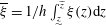 $\overline{{\it\xi}}=1/h\int _{{\displaystyle\mathop{z}\limits_{{\sim}}}}^{\widetilde{z}}{\it\xi}(z)\text{d}z$
. Assuming that the velocity profile remains similar to the equilibrium profile even for non-equilibrium flows, the shape function (2.7) can be used to work out the momentum flux
 $h\overline{u^{2}}=\int _{{\displaystyle\mathop{z}\limits_{{\sim}}}}^{\widetilde{z}}u^{2}\text{d}z=(77/48)h\overline{u}^{2}$
. Substituting this result and the constitutive relations for
 ${\it\tau}$
and
 ${\it\tau}_{W}$
, we obtain the depth-integrated momentum balance equation in the explicit form
 $$\begin{eqnarray}\frac{\partial }{\partial t}(h\overline{u})+\frac{\partial }{\partial x}\left(\frac{77}{48}h\overline{u}^{2}\right)=-g_{_{\bot }}h\frac{\partial \widetilde{z}}{\partial x}-\frac{{\it\mu}_{W}}{W}g_{_{\bot }}h^{2},\end{eqnarray}$$
where the terms
 $g_{_{\Vert }}h$
and
 ${\displaystyle\mathop{{\it\tau}_{0}}\limits_{{\sim}}}/{\it\rho}$
have cancelled each other out thanks to our choice of reference inclination
 ${\it\alpha}$
such that
 $\tan {\it\alpha}={\it\mu}_{0}$
. Equations similar to (2.9) and (2.11) have earlier been proposed to describe flows over rigid boundaries (Savage & Hutter Reference Savage and Hutter1991; Gray & Edwards Reference Gray and Edwards2014) and erodible beds (Tai & Kuo Reference Tai and Kuo2008; Lê & Pitman Reference Lê and Pitman2010).
Over rigid boundaries, depth-integrated equations obtained in this way provide a complete macroscopic description of the dynamics of open-channel flows. Over erodible beds, however, the description suffers from two blind spots. First, evolution of the two variables
 $\widetilde{z}={\displaystyle\mathop{ z}\limits_{{\sim}}}+h$
and
 $q=h\overline{u}$
does not suffice to determine the three degrees of freedom
 ${\displaystyle\mathop{z}\limits_{{\sim}}}$
,
 $h$
and
 $\overline{u}$
. Recent works have sought to address this problem by complementing (2.9) and (2.10) with an additional closure relation for the erosion rate
 $e=-\partial {\displaystyle\mathop{z}\limits_{{\sim}}}\,/\partial t$
(Tai & Kuo Reference Tai and Kuo2008; Lê & Pitman Reference Lê and Pitman2010; Iverson Reference Iverson2012). In order to deduce rates of erosion or entrainment
 $e$
from first principles, we wish to avoid this tactic. The second problem with (2.10) is that, after depth integration, only the basal internal shear stress
 ${\displaystyle\mathop{{\it\tau}}\limits_{{\sim}}}$
remains. Because the shear rate vanishes at the base, moreover, so does the rate-dependent component of the shear stress there,
 ${\displaystyle\mathop{{\it\tau}_{1}}\limits_{{\sim}}}=0$
. Hence nowhere in (2.9) and (2.10) does
 ${\it\tau}_{1}$
play any role. As a result, the equations cannot recover the equilibrium mean velocity (2.8), controlled by the rate-dependent shear stress via the rheological parameter
 ${\it\chi}$
.
To address these problems, we propose to complement (2.9) and (2.10) with an additional evolution equation expressing the balance of kinetic energy. We derive this equation by integrating (2.2) once more, this time weighted by the local velocity
 $u(z)$
, to obtain
 $$\begin{eqnarray}\frac{\partial }{\partial t}\left(\frac{1}{2}h\overline{u^{2}}\right)+\frac{\partial }{\partial x}\left(\frac{1}{2}h\overline{u^{3}}\right)=g_{_{\Vert }}h\overline{u}-g_{_{\bot }}h\overline{u}\frac{\partial \widetilde{z}}{\partial x}-\frac{1}{{\it\rho}}h\overline{{\it\tau}\dot{{\it\gamma}}}-\frac{2}{{\it\rho}W}h\overline{{\it\tau}_{W}u},\end{eqnarray}$$
where boundary conditions and the Leibniz integral rule have again been invoked. In this equation, the left-hand terms give the rate of change of the depth-integrated kinetic energy, and the divergence of the kinetic energy flux. The right-hand terms are the gravitational production, the work of the normal stress gradient and the rates of energy dissipation by internal and wall shear stresses. It should be noted that (2.2) could be multiplied by any weight function
 ${\it\omega}(z)$
prior to integration over depth. The alternative weight function
 ${\it\omega}(z)=z-(\,\widetilde{z}-(1/2)h)$
, for example, could be used to derive an equation for the balance of angular momentum about mid-depth (Steffler & Jin Reference Steffler and Jin1993). As in Richard & Gavrilyuk (Reference Richard and Gavrilyuk2013), however, the kinetic energy equation produced by the choice
 ${\it\omega}(z)=u(z)$
turns out to be particularly tractable and straightforward to interpret. Upon substituting the constitutive relations and evaluating integrals using the velocity profile (2.7), all terms of (2.12) can be explicitly worked out to obtain
 $$\begin{eqnarray}\frac{\partial }{\partial t}\left(\frac{77}{96}h\overline{u}^{2}\right)+\frac{\partial }{\partial x}\left({\it\kappa}h\overline{u}^{3}\right)=-g_{_{\bot }}h\overline{u}\frac{\partial \widetilde{z}}{\partial x}-\frac{35}{9}{\it\chi}Dg_{\bot }^{1/2}\frac{\overline{u}^{2}}{h^{1/2}}-\frac{5}{9}\frac{{\it\mu}_{W}}{W}g_{_{\bot }}h^{2}\overline{u},\end{eqnarray}$$
where
 ${\it\kappa}=(342\,853/233\,376)\approx 1.469$
. This one additional balance equation turns out to solve the different problems. By tracking the kinetic energy
 $k=(77/96)h\overline{u}^{2}$
in addition to the momentum
 $q=h\overline{u}$
and surface elevation
 $\widetilde{z}$
, we can retrieve all three degrees of freedom
 $\overline{u}=(96/77)k/q$
,
 $h=q/\overline{u}$
and
 ${\displaystyle\mathop{z}\limits_{{\sim}}}=\widetilde{z}-h$
. The rate-dependent shear stress
 ${\it\tau}_{1}$
, moreover, now intervenes via the depth-averaged dissipation term
 $\overline{{\it\tau}_{1}\dot{{\it\gamma}}}=(35/9){\it\rho}{\it\chi}Dg_{\bot }^{1/2}\overline{u}^{2}h^{-3/2}$
. As a result, application of (2.11) and (2.13) to equilibrium heap flows yields the expected depth (2.6) and mean velocity (2.8). The extended equations thus admit the correct equilibrium state.
3. Application to transient heap flows
To test the equations away from equilibrium, we now apply them to transient heap flows. As in Jop et al. (Reference Jop, Forterre and Pouliquen2007), we consider a long narrow channel, tilted to a constant inclination, in which a granular layer is released from a non-equilibrium state. The granular flow then evolves to equilibrium by adjusting its velocity and depth, entraining or detraining grains in the process. Although longitudinal variations are important in many situations, including surges resulting from column collapse (Lube et al.
Reference Lube, Huppert, Sparks and Freundt2007) and roll waves (Gray & Edwards Reference Gray and Edwards2014), here we restrict our attention to uniform flows (
 $\partial h/\partial x=\partial \overline{u}/\partial x=0$
). In this case,
 $\partial \widetilde{z}/\partial t=0$
and we only need to predict the time evolutions
 $\overline{u}(t)$
and
 $h(t)$
. We consider heaps released at a given inclination
 ${\it\beta}>{\it\alpha}$
from arbitrary initial conditions
 $\overline{u}(0),h(0)$
, distinct from the equilibrium state
 $\overline{u}_{eq},h_{eq}$
associated with excess slope
 $S=\tan ({\it\beta}-{\it\alpha})$
. Dimensionless equations are obtained by normalizing the variables
 $\overline{u}_{\ast }=\overline{u}/\overline{u}_{eq}$
,
 $h_{\ast }=h/h_{eq}$
with respect to their equilibrium values, and time
 $t_{\ast }=t/t_{c}$
with respect to the characteristic time
 $$\begin{eqnarray}t_{c}=\frac{h_{eq}^{3/2}}{g_{\bot }^{1/2}{\it\chi}D}.\end{eqnarray}$$
The characteristic time (3.1) is the standard inertial time scale of free-surface flows,
 $(h_{eq}/g_{_{\bot }})^{1/2}$
, multiplied by the ratio of macroscopic to microscopic length scales
 $h_{eq}/({\it\chi}D)$
. As signalled by the dependence of
 $t_{c}$
on the rheological parameter
 ${\it\chi}$
, the time evolution of the system is governed by the pace
 $\overline{{\it\tau}_{1}\dot{{\it\gamma}}}$
at which rate-dependent shear stresses dissipate the kinetic energy.
After normalizing, (2.11) and (2.13) can be reduced to a pair of strongly coupled ODEs in
 $\overline{u}_{\ast }$
and
 $h_{\ast }$
:
 $$\begin{eqnarray}\displaystyle \frac{\text{d}\overline{u}_{\ast }}{\text{d}t_{\ast }}=\frac{95}{44}+\frac{355}{132}h_{\ast }-\frac{160}{33}\overline{u}_{\ast }h_{\ast }^{-3/2}, & & \displaystyle\end{eqnarray}$$
 $$\begin{eqnarray}\displaystyle \frac{\text{d}h_{\ast }}{\text{d}t_{\ast }}=\frac{755}{66}\overline{u}_{\ast }^{\;\,-1}\left(\frac{87}{151}-h_{\ast }\right)h_{\ast }+\frac{160}{33}h_{\ast }^{-1/2}. & & \displaystyle\end{eqnarray}$$
 $\overline{u}_{\ast }(0),h_{\ast }(0)$
. As time
 $t_{\ast }$
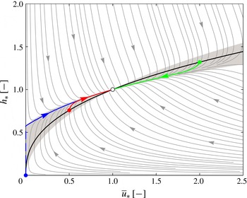
does not intervene on the right-hand side, the equations are autonomous. Their behaviour can be represented by the phase portrait of figure 2, showing system trajectories in the plane
 $(\overline{u}_{\ast },h_{\ast })$
. Starting from any point in the plane, the system evolves along prescribed curved paths which eventually converge towards the stable equilibrium point
 $(\overline{u}_{\ast },h_{\ast })=(1,1)$
. In general, the paths undergo a fast relaxation towards an attractor curve, then a slow evolution towards the equilibrium point. Within the bowtie-shaped area shown in light grey, the flowing granular layer either simultaneously entrains and accelerates (to the left of the equilibrium point), or simultaneously detrains and decelerates (to the right of the equilibrium point). Paths started from outside this area, by contrast, undergo non-monotonic evolutions in either the depth
 $h_{\ast }$
or the mean velocity
 $\overline{u}_{\ast }$
.
We now restrict our attention to transitions from one equilibrium state to another, which are straightforward to produce experimentally using a tilting flume. Under a steady feed rate, a granular flow is first driven to a stationary equilibrium state at a certain inclination
 ${\it\beta}_{1}$
, taken as the initial condition. The flume is then rapidly tilted to another inclination
 ${\it\beta}_{2}$
, triggering a transient evolution towards this new equilibrium state. By normalizing variables with respect to the target equilibrium state of angle
 ${\it\beta}_{2}$
, the corresponding dynamics can again be represented on the phase portrait of figure 2.
Phase portrait for transient heap flows showing generic system trajectories (light grey curves) and three typical trajectories (blue, red, green) started from stationary states at rest, milder and steeper inclination (initial conditions on locus
 $h_{\ast }=\overline{u}_{\ast }^{2/5}$
, black line). Light grey shading delineates the sector where both variables,
 $\overline{u}_{\ast }(t)$
and
 $h_{\ast }(t)$
, evolve monotonically.

To illustrate such transitions between equilibrium states, three sample paths with initial mean velocities
 $\overline{u}_{\ast }(0)=0,1/2,2$
are shown in figure 2 as blue, red and green lines respectively. The blue path is obtained when the granular layer starts from rest before being tilted to the target inclination
 ${\it\beta}_{2}$
. Starting from the rest state
 $(\overline{u}_{\ast }(0_{-}),h_{\ast }(0_{-}))=(0,0)$
, the flowing layer immediately jumps to the finite depth
 $h_{\ast }(0_{+})=(87/151)\approx 0.576$
(see the first right-hand term of (3.3)), then gradually thickens and accelerates towards its new equilibrium state
 $(\overline{u}_{\ast }(\infty ),h_{\ast }(\infty ))=(1,1)$
. The red path starts from a stationary flow of slower velocity. Upon being tilted to the new steeper inclination
 ${\it\beta}_{2}>{\it\beta}_{1}$
, the flowing layer rapidly thickens to approach the attractor curve, then slowly thickens and accelerates to reach its new equilibrium state. The green path starts from a stationary flow of faster velocity. Upon being tilted to the new milder inclination
 ${\it\beta}_{2}<{\it\beta}_{1}$
, the flowing layer thins and decelerates as it approaches its new equilibrium state.
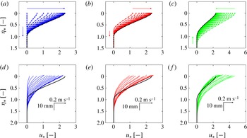
For the same three cases, we show in figure 3(a–c) the time-evolving velocity profiles
 $u(z,t)$
predicted by the depth-integrated theory. By construction, the profiles vary their mean velocity
 $\overline{u}(t)$
and depth
 $h(t)$
, but always maintain the same normalized shape (given by (2.7)). To check the validity of this approximation, we also plot evolving velocity profiles obtained by solving the local equations of § 2.1 numerically, without any recourse to depth integration, and without assuming a particular shape for the velocity profile. This is carried out using an implicit backward Euler scheme with velocity profile
 $u(z_{i},t_{k})$
discretized on a fine uniform grid
 $z_{i}$
and evolved with short time steps. The evolution of the basal boundary
 ${\displaystyle\mathop{z}\limits_{{\sim}}}(t)$
is handled by varying the number of active cells of the grid. This is taken at each time step as the maximum number of active cells that does not produce negative velocities
 $u_{i}<0$
in some of the active cells. For dimensionless times
 $t_{\ast }=0.1$
and beyond, the solutions of the depth-integrated equations are indistinguishable from these numerical solutions of the full local equations.
Velocity profiles for transient heap flows: (a–c) profiles at intervals
 ${\rm\Delta}t_{\ast }=0.1$
calculated using the depth-integrated theory (lines) and the full local equations (dots); (d–f) profiles at intervals
 ${\rm\Delta}t=0.12~\text{s}$
measured from seesaw experiments of target inclinations
 ${\it\beta}_{2}=0.479,0.473$
and 0.450. The predicted equilibrium profiles are shown in black.

4. Comparison with experiments
To check the above results, we conducted new equilibrium and non-equilibrium heap flow experiments using the seesaw channel illustrated in figure 1(c). Hinged at mid-length, the glass-walled channel (length
 $L=3~\text{m}$
, width
 $W=40~\text{mm}$
) can be tilted at different angles between runs or during flow. The channel is fed upstream by a granular hopper of adjustable aperture, with a sill at the downstream end. Equilibrium heap flow experiments were conducted by setting the upstream feed rate, then adjusting the slope until a stationary state was attained. Stationarity was checked by collecting the outflow rate at successive time intervals. Runs conducted at various feed rates and inclinations (in the range
 $24^{\circ }<{\it\beta}<28^{\circ }$
) were used to calibrate the constitutive coefficients of the theory.
Transient heap flows were produced by setting up stationary flows at a given angle
 ${\it\beta}_{1}$
, then rapidly tilting the channel (within
 $t_{2}-t_{1}=0.5~\text{s}$
) to a new inclination
 ${\it\beta}_{2}$
. For flows started from rest, the initial state was prepared instead by gradually reducing the inclination of a flowing channel until the flow was gently arrested. Flows were then started by rapidly tilting the channel back up to the desired target inclination
 ${\it\beta}_{2}$
. To aid flow initiation, the downstream sill was slightly lowered prior to tilting. The purpose of these runs was to verify the non-equilibrium behaviour predicted by the theory.
To record the equilibrium and non-equilibrium flows, we used a high-speed camera (operated at 400 f.p.s.) and particle tracking velocimetry (PTV) (Capart, Young & Zech Reference Capart, Young and Zech2002) to acquire granular velocity fields through the sidewall. Laser levelling provided a horizontal datum for elevation and inclination measurements. All experiments were conducted using quasi-monodisperse spherical ceramic millstones of diameter
 $D=2.32\pm 0.10~\text{mm}$
and density
 ${\it\rho}_{S}=2612\pm 15~\text{kg}~\text{m}^{-3}$
. Tilting table tests with millstones glued under sliding blocks were conducted to estimate the grain–glass friction coefficient
 ${\it\mu}_{W}=0.212\pm 0.005$
. For the solid fraction, we adopted the value
 $c_{S}=0.62$
applicable to quasi-monodisperse spheres (Henann & Kamrin Reference Henann and Kamrin2013).
From the equilibrium heap flow experiments, we calibrated the plastic yield coefficient
 ${\it\mu}_{0}=0.330\pm 0.012$
by fitting measurements of surface angle
 ${\it\beta}$
versus
 $q/\widetilde{u}$
, and the rheological parameter
 ${\it\chi}=0.517\pm 0.029$
by fitting measurements of
 $q^{2/7}$
versus
 ${\it\beta}$
. As in Jop et al. (Reference Jop, Forterre and Pouliquen2005), the calibrated plastic yield coefficient
 ${\it\mu}_{0}=\tan {\it\alpha}$
was significantly lower than the inclination
 $\tan {\it\beta}_{0}\approx 0.44$
at which experimental flows gently come to rest, an indication that the assumed rheology does not capture flow arrest correctly. A second value of the wall friction coefficient
 ${\it\mu}_{W}=0.200\pm 0.017$
fitted from the same data was checked to be in close agreement with the value measured in the tilting table tests (the latter was used for the calculations). We also checked that the mass fluxes
 ${\dot{m}}={\it\rho}_{S}c_{S}qW$
calculated from sidewall measurements assuming homogenous concentration
 $c_{S}=0.62$
and uniformity of the velocity profile across the width agreed with outlet measurements. We made no adjustment to the parameters when comparing model predictions against non-equilibrium heap flow experiments.
For the non-equilibrium experiments, three starting conditions were examined, corresponding, as before, to
 $\overline{u}_{\ast }(0)=0,1/2$
and 2, with each experiment repeated two or three times to ensure reproducibility. Velocity profiles
 $u(z,t)$
were averaged from PTV measurements distributed into non-overlapping bins of dimensions
 ${\rm\Delta}z\times {\rm\Delta}t=2~\text{mm}\times 30~\text{ms}$
. During channel tilt, the velocity components due to solid body rotation were subtracted from the raw measurements.
In figure 3(d–f), the measured velocity profiles for three representative runs are presented. They can be compared with the predicted time-varying profiles (figure 3
a–c) and with the predicted equilibrium profiles (plotted as black lines in figure 3
d–f). The observed profiles differ somewhat from the predicted shape (2.7). At the base, they feature thinner and deeper tails. Such creeping exponential tails, observed earlier by Komatsu et al. (Reference Komatsu, Inagaki, Nakagawa and Nasuno2001) and Jop et al. (Reference Jop, Forterre and Pouliquen2007), are not captured by the
 ${\it\mu}(I)$
rheology on which the present model is based. The maximum shear rate, on the other hand, is observed at the top of the flowing layer instead of inside the layer, one third of the depth below the free surface. As assumed by the theory, however, the profile shapes do not vary significantly during the flow evolution. Theory and experiment, moreover, are in good agreement for the time variation of the velocity and depth scales of the profiles.
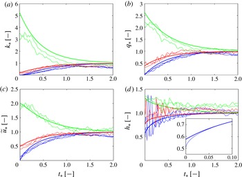
Time-evolving layer variables for transient heap flows started from rest (blue), from a slower stationary state (red) and from a faster stationary state (green): (a) depth-integrated kinetic energy
 $k_{\ast }$
; (b) momentum
 $q_{\ast }$
; (c) surface velocity
 $\widetilde{u}_{\ast }$
; (d) depth
 $h_{\ast }$
. The bold lines are the predictions from the depth-integrated theory and the thin lines are the experimental measurements, apart from the inset of (d) where the thin line is the depth calculated numerically from the full local equations.

From the PTV data, we also estimated the various layer variables and depth-integrated quantities. For each run, we used imaging measurements to identify
 $\widetilde{z}(t)$
as the elevation where the number density of imaged particles per unit wall area dropped to half its value in the static bed. Kinetic energy and momentum histories were obtained from the PTV measurements by calculating the integrals
 $k(t)=\int _{0}^{\widetilde{z}}(1/2)u^{2}\text{d}z$
and
 $q(t)=\int _{0}^{\widetilde{z}}u\text{d}z$
. The surface velocity history
 $\widetilde{u}(t)=u(\,\widetilde{z}(t))$
was obtained by sampling the measured velocity profiles at the free surface. Finally, the basal elevation
 ${\displaystyle\mathop{z}\limits_{{\sim}}}(t)$
was estimated from the condition
 $\int _{{\displaystyle\mathop{z}\limits_{{\sim}}}}^{\widetilde{z}}u\text{d}z=0.98q$
to determine the flow depth history
 $h(t)=\widetilde{z}(t)-{\displaystyle\mathop{z}\limits_{{\sim}}}(t)$
.
Comparisons with the theoretical predictions are presented in figure 4. Figures 4(a) and 4(b) show the time evolution of the depth-integrated kinetic energy and momentum, normalized by their predicted equilibrium values
 $k_{eq}({\it\beta}_{2})$
and
 $q_{eq}({\it\beta}_{2})$
and characteristic time
 $t_{c}$
. When transitioning between two equilibrium states, accelerating flows simultaneously bulk by entraining bed material. Conversely, decelerating flows thin through basal detrainment. For both entraining and detraining flows, good agreement is registered between theory and experiments. To check that the theory based on
 $q$
and
 $k$
can also recover the correct velocity and depth signals, figures 4(c) and 4(d) show results for the surface velocity
 $\widetilde{u}$
(
 $=(7/3)\overline{u}$
in the theory) and flow depth
 $h$
. Although the measurements of
 $h$
are noisier (due to the difficulty in precisely identifying the basal interface
 ${\displaystyle\mathop{z}\limits_{{\sim}}}$
), good agreement is again observed. Runs started from rest exhibit continuous evolutions for
 $\widetilde{u}$
,
 $q$
and
 $k$
, but a discontinuous jump in
 $h$
at the onset of flow. The predicted post-jump depth
 $h_{\ast }(0_{+})=(87/151)\approx 0.576$
is consistent with the earliest ascertainable values of
 $h$
in our experiments (figure 4
d, thin blue curves) and those of Jop et al. (Reference Jop, Forterre and Pouliquen2007). Closer examination of early time solutions to the full local equations, however, reveals that the correct post-jump depth should instead be
 $h_{\ast }(0_{+})=1/2$
(figure 4 d, inset). The discrepancy arises because the solution to the full local equations starts from a linear velocity profile instead of the assumed equilibrium shape. Fortunately, these profile deviations are short-lived, and the solutions to the depth-integrated and local equations become indistinguishable by time
 $t_{\ast }\approx 0.1$
.
5. Conclusion
In the present work, we derived new depth-integrated equations for entraining granular flows. By balancing the kinetic energy in addition to the mass and momentum, we showed how entrainment and detrainment can be modelled in a depth-integrated framework without recourse to an erosion law. For longitudinally uniform heap flows, solutions obtained in this way were found to agree very well with numerical solutions of the local equations, and reasonably well with laboratory experiments. The equations have yet to be tested on a greater variety of dry granular flows. For general flows varying in both space and time, numerical solvers will be required to solve the depth-integrated equations. Although not straightforward, generalization of the approach to flows unconfined by sidewalls would also be very useful. For most hazard assessment purposes, finally, it will be necessary to extend the approach to flows of liquid–granular mixtures instead of dry grains alone.
Acknowledgements
The authors are grateful for the support and advice of L. Ge from NTU, and of L. Li, A. Brügger and E. Sporer at the Carleton Laboratory, Columbia University. The research was supported by grants from the US NSF (HSEES CMMI-1331499, Geophysics/GLD EAR-1227083, GLD EAR-1148176 and GLD EAR-1124114) and by the Taiwan NSC Dragon Gate program.